Realizing three generations of the Standard Model fermions in the type IIB matrix model
Abstract:
We discuss how the Standard Model particles appear from the type IIB matrix model, which is considered to be a nonperturbative formulation of superstring theory. In particular, we are concerned with a constructive definition of the theory, in which we start with finite- matrices and take the large- limit afterwards. In that case, it was pointed out recently that realizing chiral fermions in the model is more difficult than it had been thought from formal arguments at and that introduction of a matrix version of the warp factor is necessary. Based on this new insight, we show that two generations of the Standard Model fermions can be realized by considering a rather generic configuration of fuzzy and fuzzy in the extra dimensions. We also show that three generations can be obtained by squashing one of the ’s that appear in the configuration. Chiral fermions appear at the intersections of the fuzzy manifolds with nontrivial Yukawa couplings to the Higgs field, which can be calculated from the overlap of their wave functions.
Keywords:
Matrix Models, Superstring Vacua1 Introduction
The Standard Model of particle physics is a very successful theory in that it can describe all the phenomena up to the energy scale reachable so far by accelerators. Yet it cannot be considered as a fundamental theory since it does not include quantum gravity. Also the Standard Model has quite an involved structure with many parameters, which is expected to be explained by a fundamental theory like superstring theory. Indeed there has been a lot of work in this direction with remarkable success. Superstring theory includes quantum gravity consistently, and it is a simple theory with only one scale parameter. Despite the simpleness of the theory, one can find perturbative vacua, which give rise to the Standard Model with some extra exotic particles. However, there are some serious problems as well. It seems highly nontrivial to fix all the moduli of the perturbative vacua although there are some new ideas such as the flux compactification. Moreover, it is known that there actually exist tremendously many perturbative vacua, which is a situation commonly referred to as the string landscape nowadays. From this point of view, one cannot even explain why we live in a four-dimensional space-time since perturbative vacua can have various space-time dimensionality less than or equal to ten.
Of course, all these problems might be simply because superstring theory has been studied essentially in perturbation theory including, at most, some nonperturbative effects represented by the existence of D-branes. Therefore a different picture might emerge if one studies the theory in a completely nonperturbative framework. As a well-known example, nonperturbative studies of QCD by lattice gauge theory explained important low-energy dynamics such as confinement of quarks, which can never be understood in perturbation theory. The hadron mass spectrum has been reproduced accurately by Monte Carlo calculations based on the lattice gauge theory, and such a method has been playing a crucial role in studying various properties of hadrons. Likewise it is possible that the compactification of extra six dimensions can be understood as a nonperturbative effect in superstring theory, and that the involved structure of the Standard Model and its parameters can be understood from a rather simple structure in the extra dimensions.
As a nonperturbative formulation of superstring theory, we consider the type IIB matrix model [1], which consists of 10 bosonic Hermitian matrices () and 16 fermionic Hermitian matrices (). The action of the model can be formally obtained from that of ten-dimensional SU() super Yang-Mills theory by dimensional reduction. The Yang-Mills coupling, which is the only parameter of the model, becomes just a scale parameter after the dimensional reduction since it can be absorbed by appropriate rescaling of the matrices. The type IIB matrix model has a direct connection to perturbative type IIB superstring theory, but it is expected to describe the unique nonperturbative theory of superstrings underlying the duality web of various perturbative formulations. The matrix size corresponds to the number of sites in the lattice gauge theory, which makes the dynamical degrees of freedom in the system finite. By taking the large- limit in an appropriate manner, one obtains a constructive definition of superstring theory. Nowhere in the definition does one have to make a perturbative expansion, hence it is a nonperturbative formulation. A particularly interesting aspect of the type IIB matrix model is that space-time is treated as a part of dynamical degrees of freedom in the bosonic matrices . It is therefore possible that four-dimensional space-time appears dynamically.
For more than fifteen years since its proposal, the type IIB matrix model has been studied in its Euclidean version, which can be obtained by making a “Wick rotation” . This is fine when one calculates the interactions between D-branes at the one-loop level, for instance, but the physical meaning of the “Wick rotation” is not clear at a fully nonperturbative level unlike in quantum field theory. The Euclidean version has been studied intensively, nevertheless, because it has a finite partition function [2, 3]. See refs.[4, 5] for recent work, which suggests that spontaneous breaking of the SO(10) symmetry occurs in the Euclidean matrix model.
The Lorentzian version remained untouched until recently since it looked simply ill-defined due to its non-positive-definite action. However, ref. [6] showed that the Lorentzian version can be made well-defined nonperturbatively by first introducing infrared cutoffs in both temporal and spatial directions, and then removing them in the large- limit in such a way that the continuum and infinite-volume limits are taken. The resulting theory has no parameters other than one scale parameter. Moreover, it turned out that one can extract a real-time evolution by taking an ensemble average over matrix configurations, which showed that (3+1)-dimensional expanding universe emerges dynamically. This provides a strong evidence that the Lorentzian version of the type IIB matrix model indeed describes the unique nonperturbative theory of superstrings, and that the theory provides a natural explanation for the origin of our 4-dimensional space-time.
The aim of the present work is to discuss whether the same theory can also provide a natural explanation for the origin of the Standard Model. In particular, the Standard Model has the following peculiar features:
- i)
The gauge interaction is governed by , which is a semi-simple group instead of being a simple one.
- ii)
The matter contents are fermions, which couple to the gauge fields in a characteristic manner. Quarks couple to the SU(3) gauge field, while leptons do not. Left-handed fermions couple to the SU(2) gauge field, while right-handed ones do not. The assignment of the U(1) hypercharge is quite involved.
- iii)
The matter contents have three generations, which couple to the gauge fields in exactly the same manner.
- iv)
The fermions have Yukawa couplings to the Higgs field. Due to the existence of three generations, the Yukawa couplings involve a lot of parameters, which can only be determined experimentally within the Standard Model.
We discuss how these features can be realized in the type IIB matrix model.
One of the biggest obstacles in obtaining the Standard Model from higher-dimensional theories like superstring theory is that the fermions should be chiral. If one applies a naive dimensional reduction to higher dimensional theories, fermions become vector-like in four dimensions. In order to realize chiral fermions, one needs to consider, for instance, (a) orbifolding, which amounts to imposing a nontrivial identification in the extra dimensions, (b) introducing intersecting/magnetized D-branes, (c) introducing a nonzero Euler number in the Calabi-Yau compactification.
Realization of chiral fermions and the Standard Model has been discussed also in the type IIB matrix model by various authors. In ref. [7] an orbifolding condition was imposed on the matrix configuration, and it was shown to give rise to a four-dimensional theory including chiral fermions. See also refs. [8, 9] for related works. Ref. [10] studies a matrix model in which the Hermitian matrices () in the extra dimensions are replaced by unitary matrices with an action obtained as a one-site model of six-dimensional SU() lattice gauge theory. These matrices can have solutions representing a 6d non-commutative torus carrying magnetic fluxes. Chiral fermions can be obtained in this background if one uses a Ginsparg-Wilson Dirac operator, which has an exact modified chiral symmetry. One can realize three generations of the Standard Model particles by choosing the fluxes in the 6d torus appropriately.11 1 As a closely related work, refs. [11, 12] discuss realization of the Standard Model by toroidal compactification of ten-dimensional SU() super Yang-Mills theory with orbifold conditions. Realistic CKM and PMNS matrices were obtained by choosing the vacuum expectation values of such quantities as Wilson lines, the Kähler moduli, the complex-structure moduli and the dilaton [11]. The probability distribution for the appearance of the Standard Model and other phenomenological models has been calculated in this setup [13, 14].
While the above proposals attempt to realize chiral fermions by modifying the model, ref. [15] proposed to realize chiral fermions in the original type IIB matrix model based on the idea of intersecting branes [16], which has been explored extensively in the phenomenological context [17, 18, 19, 20, 21, 22, 23, 24, 25, 26]. It was shown that chiral fermions indeed appear at the intersections when the branes are given by (hyper)planes [27], which can be represented by operators or infinite dimensional matrices in the matrix model. The authors then proposed to replace these branes by fuzzy spheres and other fuzzy manifolds, which can be represented by finite- matrices. Realization of the Standard Model has also been discussed.
Recently, two of the authors (J.N. and A.T.) [28] calculated explicitly the spectrum of the Dirac operator for a finite- configuration suggested in ref. [15], which represents a 5-brane and a 7-brane intersecting at a point in the extra dimensions. It was confirmed that a chiral zero mode localized at the intersection point indeed appears in the large- limit. However, one also obtains another chiral zero mode with opposite chirality, which was not anticipated naively from the brane configuration. This result was understood as a consequence of a no-go theorem, which states that chiral fermions cannot be realized in the large- limit of finite- type IIB matrix model as far as one assumes that space-time is given by a direct product of our four-dimensional space-time and the space in extra six dimensions. In fact, the SO(3,1) Lorentz symmetry alone does not imply the direct product structure of space-time, and one generally obtains a warp factor. In a generic case with a nontrivial matrix representing a warp factor, chiral zero modes in extra six dimensions do not automatically correspond to those in our four-dimensional space-time. For the above explicit configuration, it was found that there are huge degrees of freedom in , which allows only the desired chiral zero mode to appear in four dimensions [28]. Thus one can realize a chiral fermion in the large- limit of finite- type IIB matrix model thanks to the matrix warp factor .
The no-go theorem and the need for introducing a nontrivial to avoid its consequence affect drastically the discussions on the possibilities of realizing chiral fermions and the Standard Model in the type IIB matrix model. In particular, the new insights enable us to realize chiral fermions from intersecting fuzzy and fuzzy , which can be obtained as classical solutions in the type IIB matrix model assuming that a Myers term [29] is induced dynamically. (See refs. [30, 31, 32], which discuss the appearance of these fuzzy manifolds in the type IIB matrix model due to quantum corrections. Note also that, including the dimensionality of our 4d space-time, fuzzy and fuzzy correspond to a D5-brane and a D7-brane, respectively, which naturally appear in type IIB superstring theory.) The two types of fuzzy manifold intersect in the six-dimensional space generically at even number of points, which give rise to pairs of chiral fermions with opposite chirality in six dimensions. However, by using the degrees of freedom in the matrix warp factor , one can obtain only the desired chiral zero modes in four dimensions.
Extending this basic setup, we discuss an explicit realization of the Standard Model. The SU() group can be realized as a subgroup of U(), which appears naturally from coinciding branes. First we introduce “SU(3) branes”, which consist of three coinciding fuzzy , and “SU(2) branes”, which consist of two coinciding fuzzy . In addition, we introduce a “lepton brane”, which is a single fuzzy , and an “up-type brane” and a “down-type brane”, which are two separate fuzzy . Thus we end up with a configuration with five stacks of branes intersecting with each other. An important point here is that chiral fermions actually appear only from intersections of fuzzy and fuzzy . This enables us to obtain just the chiral fermions in the Standard Model plus a right-handed neutrino, with the correct gauge interactions. One can also check that the hypercharge can be assigned to the chiral fermions consistently.
In fact, we show that the number of intersections of and in six dimensions cannot exceed four for arbitrary radii, location of the centers and their relative angles. This implies that we can obtain only up to two generations if we restrict ourselves to such configurations. Three generations can be realized, for instance, by squashing or that appear in the configuration. We also discuss how the Higgs field appears from the bosonic matrices, with nontrivial Yukawa couplings to the Standard Model fermions. Thus we find that all the peculiar features i)–iv) of the Standard Model listed above can be explained from a rather simple structure in the extra dimensions within the type IIB matrix model. The main results of this paper was reported by A.T. at the Workshop on Noncommutative Field Theory and Gravity, 8-15 September 2013 held in Corfu, Greece.
The rest of this paper is organized as follows. In section 2 we briefly review how chiral fermions can be realized in the type IIB matrix model following ref. [28]. In section 3 we discuss the emergence of chiral fermions from a basic configuration, which consists of fuzzy and fuzzy . In section 4 we discuss how one can realize the Standard Model fermions by considering a matrix configuration corresponding to five stacks of branes. In section 5 we discuss the number of generations that can be realized within this setup. In section 6 we discuss how the gauge field and the Higgs field appear from the model. In particular, we discuss how nontrivial Yukawa couplings can be obtained from the overlap of wave functions. Section 7 is devoted to a summary and discussions.
Note Added: While we were preparing the manuscript, we encountered a preprint [33], which has certain overlap with our paper.
2 Realizing chiral fermions in the type IIB matrix model
The type IIB matrix model has an action [1]
| (1) | |||||
| (2) | |||||
| (3) |
where are gamma matrices in 10d. The bosonic matrices () are traceless Hermitian, while the fermionic matrices () are Majorana-Weyl fermions in 10d, and, in particular, they satisfy
| (4) |
where is the chirality operator in 10d. Since the coupling constant can be absorbed by rescaling and appropriately, it is merely a scale parameter.
The type IIB matrix model is conjectured to be a nonperturbative definition of superstring theory [1]. There are various pieces of evidence for this conjecture. First of all, the action (1) can be regarded as a matrix regularization of the worldsheet action of type IIB superstring theory in the Schild gauge [1].22 2 This does not imply that the matrix model is merely a formulation for the “first quantization” of superstrings. In fact, multiple worldsheets appear naturally in the matrix model as block-diagonal configurations, where each block represents the embedding of a single worldsheet into the 10-dimensional target space. Secondly, D-branes in type IIB superstring theory can be described as simple matrix configurations, and the interaction between them can be reproduced correctly [1]. Thirdly, under a few reasonable assumptions, the string field Hamiltonian for type IIB superstring theory can be derived from Schwinger-Dyson equations for the Wilson loop operators, which are identified as creation and annihilation operators of strings [34].
In all these connections to type IIB superstring theory, the target space coordinates are identified with the eigenvalues of the matrices [35]. In particular, this identification is consistent with the supersymmetry algebra of the model, in which the translation that appears from the anti-commutator of supersymmetry generators is identified with the shift symmetry of the model, where . Also the fact that the model has extended supersymmetry in ten dimensions is consistent with the assertion that the model actually includes gravity since it is known in field theory that supersymmetry is the maximal one that can be achieved in ten dimensions without including gravity.
Below we review the general arguments in ref. [28] concerning the appearance of chiral fermions in 4d from the type IIB matrix model. In this model, the space-time is represented by the ten bosonic Hermitian matrices (). As it was shown by ref. [6], an expanding three-dimensional space appears dynamically after some time. At later times, it is speculated that three-dimensional space becomes much larger than the typical scale of the model, and that quantum fluctuations can be neglected at large scales [36, 37]. Furthermore, as far as we do not consider too long time scale, we can neglect the expansion of space and therefore the space-time has SO(3,1) Lorentz symmetry. Thus we are led to consider matrix configurations given by
| (5) | ||||
| (6) |
Here we assume that the Hermitian matrices have the property , where and . Then (5) and (6) can be regarded as the most general configuration that is SO(3,1) invariant up to symmetry.
The Hermitian matrix in (5) can be regarded as a matrix version of the warp factor. The special case corresponds to a space-time which is a direct product of (3+1)-dimensional space-time and the extra dimensions. However, from the viewpoint of preserving the Lorentz symmetry, there is no reason to set .
In order to discuss chiral fermions in 4d, it is convenient to decompose the gamma matrices in 10d into the ones in 4d and 6d as
| (7) |
where and are gamma matrices in 4d and 6d, respectively, which satisfy
| (8) |
and is the chirality operator in 4d. Note that the chirality operator in 10d can be decomposed as
| (9) |
where is the chirality operator in 6d.
In the case of quantum field theory in higher dimensions, one decomposes fields into Kaluza-Klein modes, which can then be identified as four-dimensional fields. Here we make a similar analysis in the language of matrices.33 3 See ref. [38] for discussions on the appearance of local field theory in the Lorentzian type IIB matrix model. We consider expanding the fermionic variables in terms of the eigenmodes of the Dirac operator in 6d defined by
| (10) |
In the explicit example to be discussed in the next section, we consider a configuration of , which has a block diagonal form
Correspondingly, we decompose in eq. (10) as
Since the Dirac operator acts on each block independently, the eigenvalue problem for can be decomposed into that in each block.
As we will see in the explicit example, chiral fermions actually appear in off-diagonal blocks. Therefore, from now on, we consider the eigenvalue problem for , which is given by
| (15) |
Due to the fact that and are Hermitian matrices, one can easily show that the eigenvalue in (15) is real. Also, by multiplying to (15) from the left, one obtains
| (16) |
This implies that if is an eigenvector with the eigenvalue , is an eigenvector with the eigenvalue . In particular, and are linearly independent for . Therefore we can construct left-handed and right-handed modes by taking linear combinations of and with as
| (17) |
which satisfy
| (18) |
and
| (19) |
Thus the non-zero modes appear in pairs of right-handed and left-handed modes. On the other hand, the zero modes can be assumed to have definite chirality. Since we are considering finite- matrices, the space of with each chirality has the same dimension. Therefore, the number of zero modes with each chirality should also be the same. However, the actual form of the zero mode with each chirality can be very different in general. This fact will be important in getting chiral fermions in 4d.
Let be a set of non-negative eigenvalues in (15). Then we denote the right-handed and left-handed modes corresponding to by and , respectively. These modes can be normalized in such a way that they satisfy the orthonormal condition
| (20) |
where the labels and represent either or .
Now we decompose the fermionic variables in (3) in the same way as in (2), and expand the off-diagonal block in terms of the orthonormal basis and constructed above as
| (21) |
Note that the matrix coefficients and introduced here satisfy
| (22) |
as one can see from (4), (9) and (18). Namely, the left-handed and right-handed modes in 6d correspond to the left-handed and right-handed modes in 4d, respectively. Note also that the other off-diagonal block is related to the off-diagonal block that we have considered through charge conjugation as
| (23) |
due to the Majorana condition for . This allows us to focus only on .
In what follows we consider the case in which the matrix warp factor in (5) has a block diagonal form similar to (2) as
Then, by substituting (21) into the action (3), we find that the case , namely the case with and in (2), leads to vector-like fermions in 4d [28]. (See also footnote 9.) Therefore we find that in order to obtain chiral fermions, we need to consider and nonvanishing . In particular, let us consider the case with and for . Suppose and satisfy
| (26) |
for the left-handed mode , but not for the right-handed mode . Then, we find that has an appropriate form of the action as a chiral fermion in 4d, and it does not couple to the other modes [28]. On the other hand, does not have an appropriate form of the action as a chiral fermion in 4d, and it couples to the massive modes with . This implies that we obtain only a left-handed chiral fermion in 4d. While we do not know at present the mechanism that favors the matrix satisfying (26) for only one of the chiralities, we will argue that all the chiral fermions in the Standard Model can be obtained in this way by using the huge degrees of freedom in .
3 A basic configuration with fuzzy and fuzzy
As an example of , which allows nontrivial solutions to (15) with , we consider an explicit finite- configuration given by
where we have defined
| (39) |
Here, the matrices () are the -dimensional irreducible representation of the SU(2) algebra , which represents a fuzzy sphere
| (40) |
with the radius . The top-left block and the bottom-right block in eq. (3) represent fuzzy and fuzzy , respectively, and eq. (39) amounts to shifting them in some directions. Including the dimensionality in four-dimensional space-time, these fuzzy manifolds correspond to a D5-brane and a D7-brane, respectively, which appear naturally in type IIB superstring theory.
The intersections of the two fuzzy manifolds in eq. (3) can be obtained easily. The classical manifold corresponding to the fuzzy is represented by
| (41) |
whereas that corresponding to the fuzzy is represented by
| (42) |
Solving (41) and (42) simultaneously, we obtain and with , which represent two intersecting points in the 6d space. At the two intersecting points, we obtain chiral fermions with opposite chirality. The situation is depicted on the -plane in figure 1.

The configuration (3) looks similar to the one studied in ref. [28] following the original proposal [15]. However, there are some important differences in the bottom-right block. The in eq. (17) of ref. [28] involves . This implies that the bottom-right block in ref. [28] does not represent a fuzzy , and hence it cannot be obtained as a classical solution in a matrix model with a Myers term. Moreover, the extent of the configuration in ref. [28] diverges in the -direction when one takes the large- limit. On the other hand, the configuration (3) is completely finite in the large- limit. This is more natural in view of the results obtained by Monte Carlo simulation [6], which show that the extent in the six dimensions remains finite and small.
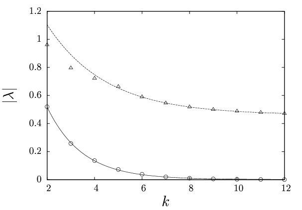
We would like to solve the eigenvalue problem for the Dirac operator in 6d defined by (10) with given above. Due to the block diagonal structure of , we can decompose into blocks as (2), and the problem reduces to solving the equation for each block. On physical grounds, it is expected that chiral zero modes appear from the off-diagonal blocks, which correspond to the degrees of freedom connecting the two different branes. Thus the problem reduces to solving the eigenvalue equation (15). As we explained below eq. (16), eigenvalues appear in pairs with opposite signs. In figure 2 the smallest and the second smallest one are plotted against . We find that the smallest one vanishes rapidly with increasing , which implies the appearance of two zero modes in the large- limit. The second smallest , on the other hand, seems to approach a non-zero constant.
Let us take an appropriate linear combination of the two modes with the smallest so that they have definite chirality as we have done in eq. (17). Figure 3 shows the shape of the wave function
| (43) |
of the chiral mode with each chirality for . Let us recall here that represents the top-right block in (2). In the eigenvalue equation (15), the matrices act on the index , whereas the matrices act on the index . In the present configuration (3), and represent the fuzzy and the fuzzy , respectively. Below we explain some conventions used to make the plots in figure 3. First, as a -dimensional representation of the algebra in the configuration (3), we use
| (44) |
Second, when we make a tensor product in the bottom-right block in (3), we combine the indices as with and . In this way, the indices and of the wave function correspond to the eigenvalues of in the fuzzy and the fuzzy , respectively.


From figure 3 (Left) we find that the left-handed chiral mode has a peak at . With the chosen conventions, corresponds to the point on the fuzzy (41), whereas corresponds to the point and on the fuzzy (42). Thus we find that the wave function of the left-handed chiral mode is localized at one of the intersection points in figure 1.
On the other hand, from figure 3 (Right), we find that the wave function of the right-handed chiral mode does not seem to be localized.44 4 In fact, the wave function is suppressed at , which implies that it is localized at on the second of (42). However, this is simply due to the chosen representation of the SU(2) algebra. For instance, let us make a replacement
| (45) |
in the fuzzy , and a replacement
| (46) |
in the first of the fuzzy . The shape of the wave function (43) with this representation is shown in figure 4. We find that the right-handed chiral mode has a peak at . With the new convention, corresponds to the point on the fuzzy (41), whereas corresponds to the point and on the fuzzy (42). This implies that the wave function of the right-handed chiral mode is localized at one of the intersection points in figure 1. Thus, in order to see that chiral modes are localized on the intersection points from the profile of the wave function, one generally needs to choose the representation of the SU(2) algebra for each chiral mode appropriately.


In the original representation (3) with (44), the left-handed chiral mode takes a simple form
at large , where . Note that (3) is a matrix. The matrices and which satisfy (26) for this mode in the large- limit are given by
which are and Hermitian matrices, respectively. In the same representation, the wave function of the right-handed chiral mode is quite different from (3), and it does not satisfy (26) generically. Thus we can obtain a single chiral zero mode in four dimensions.

4 Realizing the Standard Model fermions
In this section we discuss how to realize the Standard Model fermions extending the basic setup in section 3.
First we introduce gauge symmetry by replacing each of the branes by coincident multiple branes similarly to the case of D-brane effective theory. For instance, if we make a replacement
| (60) |
in the configuration (2), we obtain gauge symmetry as a subgroup of the U() symmetry of the original model. Then the chiral zero mode that appears from the top-right block in (2) becomes a bi-fundamental representation .
In order to realize the Standard Model fermions, we consider a matrix configuration with five diagonal blocks, , which correspond to five stacks of branes. First we introduce “SU(3) branes”, which consist of three coinciding fuzzy , and “SU(2) branes”, which consist of two coinciding fuzzy . In addition, we introduce a “lepton brane”, which is a single fuzzy , and an “up-type brane” and a “down-type brane”, which are two separate fuzzy . Thus we end up with a configuration with five stacks of branes55 5 An analogous configuration was discussed in section 4.2 of ref. [15], but it was dismissed for a reason that does not apply to our case. depicted in figure 5.
| 1/6 | 2/3 | -1/3 | -1/2 | 0 | -1 | |
| 1/3 | 1/3 | 1/3 | 0 | 0 | 0 | |
| 0 | 0 | 0 | 1 | 1 | 1 | |
| 1 | 0 | 0 | 1 | 0 | 0 | |
| 0 | 1 | 1 | 0 | 1 | 1 |
| 1/6 | -1/2 | 0 | -1/2 | 1/2 | |
| 1/3 | 0 | 0 | 0 | 0 | |
| 0 | 1 | 0 | 0 | 0 | |
| 0 | 0 | -1 | 0 | 0 | |
| 0 | 0 | 0 | -1 | -1 |
In fact, chiral fermions appear only from intersections of fuzzy and fuzzy in generic situations in six dimensions. Note first that and have six dimensions in total, and therefore they intersect with each other at some points in six dimensions generically. On similar grounds, two do not intersect with each other. Two intersect, but on a two-dimensional surface. In this case, the index in six dimensions vanishes unless a nontrivial flux is induced on the surface. Thus, it is possible to obtain just the chiral fermions in the Standard Model plus a right-handed neutrino, with the correct gauge interactions.66 6 For this purpose alone, one may exchange the roles of and simultaneously. We prefer the present version, which makes our discussion on the Higgs field simpler. One can easily see that the chiral fermions have the correct representations under the gauge group SU(3) SU(2).
The hypercharge can also be assigned to the fermions correctly. Each stack of branes produces a U(1) gauge group. Let () be the U(1) charge associated with the -th stack of branes. An open string connecting the -th and -th stacks of branes, which is represented by the off-diagonal block connecting the -th and -th diagonal blocks, has and . Therefore, if we define a charge as the linear combination
| (61) |
the chiral fermion that appears at the intersection of the -th and -th stacks of branes has . By appropriately choosing the coefficients , one can assign the correct hypercharge to the chiral fermions appearing at all the intersections. Other choices of the coefficients define other U(1) charges such as the baryon number , the lepton number , the left-handed charge and the right-handed charge . The charges for each chiral fermion and the values of the coefficients for each charge are given in table 1.
As is well known in quantum field theory, the U(1) gauge symmetries other than and are anomalous with the above contents of chiral fermions. In the intersecting D-brane models in string theory, these anomalies are canceled by the Green-Schwarz mechanism. This occurs due to the exchange of the Ramond-Ramond field, which also makes the anomalous U(1) gauge fields and some of the anomaly-free gauge fields massive. We speculate that a similar mechanism works in the matrix model as well.
5 The number of generations
If all the intersections of and in the configuration in figure 5 are similar to (3), we get only one generation of the Standard Model fermions. In section 5.1 we show a simple example in which one can get two generations by modifying the configuration (3). In section 5.2 we generalize the argument and show that one cannot get more than two generations by changing the radii of the ’s in the configuration or by shifting/rotating the fuzzy manifolds relatively. In section 5.3 we show that three generations can be obtained by squashing one of the of the in the configuration.
5.1 Two generations—a simple example

In order to get a simple example of configurations giving rise to two generations, let us multiply a factor to , , corresponding to the second of the fuzzy in (3). Then eq. (42) is replaced by
| (62) |
For , the (41) and the (62) intersect not only on but also on . Slicing the six-dimensional space by these two hyperplanes, we obtain a view depicted in figure 6 on the -plane. The small circle that appears from has a radius , and it intersects with another circle when , i.e., as shown in figure 6. In this case, the and the intersect at four points, giving rise to two pairs of chiral fermions with opposite chirality. In what follows we take as an example.
We solve the eigenvalue equation (15) for this configuration and plot the three smallest against in figure 7. We observe that two of them vanish rapidly as increases, which suggests the appearance of two pairs of chiral zero modes.77 7 The exponential fit in figure 7 seems to suggest that the second smallest asymptotes to a small but finite number. This is also the case with the third smallest for the three-generation case shown in figure 10. Whether this leads to a practical problem or not deserves further investigations.

We take an appropriate linear combination of the two modes with the smallest so that they have definite chirality as we have done in eq. (17). We also do the same thing for the two modes with the second smallest . In figure 8 we show the wave functions of these chiral zero modes. The plots at the top correspond to the smallest , which look quite similar to the plots in figure 3. These modes are essentially the ones that appeared in section 3. The plots at the bottom correspond to the second smallest . These modes are the ones that appear from the additional intersections using the small circle in figure 6. Correspondingly, the wave functions have non-zero values within the region , which corresponds to the “north pole” of the second of the . In particular, the right-handed mode is localized at as anticipated. In the chosen basis, we find that the chiral zero modes that appear near are seen to be manifestly localized. As we did in section 3, we can change the basis in such a way that the ones that appear near are seen to be manifestly localized.


By using the warp factor again, we can get two generations of the left-handed fermions. First we restrict ourselves to the form (3) in order to get the left-handed mode localized at . Next we change the basis in such a way that the left-handed mode appearing near are seen to be localized at . Then we require that the warp factor in that basis should have the form (3). Note that this requirement is compatible with (3) in the original basis since there are a lot of degrees of freedom left arbitrary in (3). In fact, the number of degrees of freedom in and are and , respectively, whereas the restriction to the form (3) in a particular basis requires only and for and , respectively.
5.2 Generalization
As we have seen above, the number of generations can be deduced only from geometric arguments. Let us therefore consider a general configuration of fuzzy and fuzzy , which can be obtained from the basic configuration (3) by changing the radii of the ’s that appear in the configuration and by shifting/rotating the fuzzy manifolds relatively. Without loss of generality, we assume that the classical manifold corresponding to the fuzzy is represented by
| (63) |
and that corresponding to the fuzzy is represented by
| (64) |
We have introduced
| (65) |
where is a matrix representing a general six-dimensional rotation, and is a six-dimensional vector, which represents a general shift. In order to obtain the intersections, we solve (63) and (64) simultaneously. Let us decompose the matrix , the vector and the six-dimensional coordinate as
Since , we have a constraint , which reads
| (72) |
In order to obtain the intersections, we may restrict ourselves to due to (63). Then we have to solve
| (73) | ||||
By adding (5.2) and (5.2) and using (72), we obtain
| (82) |
| (83) |
Thus the problem reduces to solving (73), (5.2) and (83) simultaneously. The intersection of (73) and (83) gives a circle, while the intersection of (5.2) and (83) gives an ellipse. Note that a circle and an ellipse on the same plane cannot intersect at more than four points. Therefore, we can obtain only up to two generations as far as we restrict ourselves to a general configuration of fuzzy and fuzzy .


5.3 Three generations from squashed
In order to get three generations, we need to go beyond the class of configurations considered in section 5.2. In general, the dominant background can be different from such a configuration in various ways. Here we show that one can actually obtain three generations by squashing one of the of the fuzzy in the configuration.88 8 It remains to be seen whether such configurations with squashed fuzzy spheres can be realized as solutions to the equation of motion with possible dynamically generated terms like the Myers term. As an example, we consider a case in which the is represented by
| (84) |
and the is represented by
| (85) |
We solve (84) and (85) simultaneously. First we find that or . Then the problem reduces to solving
| (86) | ||||
| (87) |
simultaneously. Eq. (86) represents two co-centered circles, while eq. (87) represents an ellipse. By choosing the parameters as
| (88) |
we obtain the situation depicted in figure 9 on the -plane.
We solve the eigenvalue equation (15) for this configuration and plot the four smallest against in figure 10. We observe that three of them vanish rapidly as increases, which suggests the appearance of three pairs of chiral zero modes.


We take an appropriate linear combination of the two modes with the smallest so that they have definite chirality as we have done in eq. (17). We also do the same thing for the two modes with the second smallest , and similarly for the third smallest . In figure 11 we show the wave functions of these chiral zero modes. The plots at the top correspond to the smallest . They are peaked near and , respectively. These are the modes that are localized at the intersection points in figure 9. The plots in the middle row correspond to the second smallest . These modes are the ones that appear due to the squashing. They have non-zero values for , which corresponds to the “north pole” of the first of the and the “south pole” of the second of the . The plots at the bottom correspond to the third smallest . They have non-zero values for , which corresponds to the “south pole” of the first of the and the “north pole” of the second of the .
Similarly to the discussion at the end of section 5.1, we can get three generations of the left-handed fermions by using the warp factor . The crucial point is that we can always choose a basis in such a way that the wave function of each generation of the left-handed fermion looks like (3). The number of arbitrary elements in (3) is so large that one can impose the condition for each generation without conflicts.
6 Interactions with the gauge field and the Higgs field
In this section we discuss how the Standard Model fermions that appear in the model interact with the gauge field and the Higgs field.
The gauge field is expected to appear from the fluctuation of around (5), which we decompose as . Since the gauge field should be a zero mode, we obtain in the Lorentz gauge. This results in a block diagonal with and for the explicit example of in (3). The gauge field is therefore insensitive to the wave function in the extra dimensions.99 9 This also implies that in the case the chiral zero modes with opposite chirality that appear from the same block interact with the gauge field in the same manner. Thus we obtain a vector-like gauge theory in that case. This guarantees the universality of the gauge coupling.
Similarly the Higgs field is expected to appear from the fluctuation of () around (6), which we decompose as . The spectrum of the fluctuation is obtained by
| (89) |
in the Lorentz gauge. As a massless mode, one always has a block diagonal with and for the explicit example of in (3). In the case of the configuration with five stacks of branes in section 4, we obtain massless adjoint scalars, which do not couple to the Standard Model fermions due to the Lorentz symmetry.
On top of this, one can obtain light scalar modes from the off-diagonal block connecting two of the fuzzy ’s in the configuration when the two spheres come close to each other. If the branes come close to the up-type brane, one obtains a scalar, which has Yukawa couplings to the SU(2) doublets and the up-type fermions. Similarly, if the branes come close to the down-type brane, one obtains a scalar, which has Yukawa couplings to the SU(2) doublets and the down-type fermions. In the Standard Model, these two scalar fields are related to each other by G-parity, but in the present case we obtain them as independent fields as in the two-Higgs-doublet model1010 10 See ref. [39] for a review. Using their notation, our situation corresponds to the type II model among the four types of the model which avoids the tree-level flavor changing neutral current. This type of the two-Higgs-doublet model has been studied intensively since it is the structure that appears in the Minimal Supersymmetric Standard Model. . If the up-type brane comes close to the down-type brane, one obtains an SU(2) singlet scalar. Since the Standard Model fermions localized on these branes are both right-handed, however, this scalar field does not couple to the Standard Model fermions due to the Lorentz symmetry. Note also that since has six components, we have six copies of light scalar particles. Their couplings to the Standard Model fermions are different, however, since SO(6) symmetry is broken completely by the background configuration.
In general, all the scalar modes acquire mass through radiative corrections, and decouple from the low-energy spectrum. We consider that the one that couples most strongly to top quarks (and right-handed neutrinos) gets radiative correction to with minus sign, and eventually induces the electroweak symmetry breaking. Thus we obtain only the Standard Model Higgs particle at low energy although we have many more scalar particles with or without Yukawa couplings to the Standard Model fermions at high energy.
As an example, let us consider the Higgs particle that appears when the SU(2) branes and the up-type brane come close to each other. We can calculate the Yukawa couplings to the quark doublets and the right-handed up-type quarks using the three-point coupling (3) in the type IIB matrix model. The matrix representing the Yukawa couplings can be obtained simply from the overlap of the wave functions as
| (90) |
where represents the generation and represents the gamma matrices in 6d. The index corresponds to the six copies of the Higgs particles. The matrix represents the off-diagonal block of the matrix in (89) connecting the SU(2) branes and the up-type brane.
If one considers an extreme case in which the two coincide with each other, (89) has a zero mode for . As far as the two are close, we obtain a light Higgs particle with . Whether we can obtain a realistic structure of the Yukawa couplings by choosing the background configuration appropriately is an interesting open question.
7 Summary and discussions
In this paper we discussed how the Standard Model appears from the type IIB matrix model. While this issue has been discussed by many authors, the novelty of our discussion is that we take the model as it is without any modifications, and that we consider a constructive definition starting from finite- configurations and taking the large- limit later on. In that case, we have found in ref. [28] that realizing chiral fermions is much more difficult than one would expect from the formal arguments at . There it was shown that chiral fermions in the extra six dimensions should appear in pairs with opposite chirality. One can, however, introduce a matrix version of the warp factor, which enables us to make only the desired chiral fermions in six dimensions correspond to the ones in four dimensions. This is always possible by using the huge degrees of freedom in . It remains to be seen whether the warp factor determined dynamically has the form required for the appearance of chiral fermions.
Accepting this scenario for the appearance of chiral fermions in the type IIB matrix model, we discussed whether the Standard Model appears naturally from the model. While we basically follow the idea of ref. [15] using the intersecting branes to obtain chiral zero modes at the intersections, we have shown that the Standard Model fermions appear from quite generic configurations consisting of fuzzy and fuzzy without fine-tuning. By virtue of using the two types of fuzzy manifolds with different dimensionality, we are able to obtain just the Standard Model fermions plus the right-handed neutrino.
The Higgs sector is somewhat exotic, though. We obtain the SU(2) and SU(3) adjoint massless scalars, which do not couple to the Standard Model fermions. We also have possibilities of obtaining two light scalar modes as SU(2) doublets. One of them has Yukawa couplings to the SU(2) doublets and the up-type fermions, and the other one has Yukawa couplings to the SU(2) doublets and the down-type fermions. This part resembles the two-Higgs-doublet model [39]. Another light scalar can appear as an SU(2) singlet, which does not couple to the Standard Model fermions. All these scalar modes appear with multiplicity of six due to the number of extra dimensions. We have argued a possibility that the one with the strongest Yukawa coupling to the top quark (or the right-handed neutrino) induces the electroweak symmetry breaking due to radiative corrections to , and survives in the low energy spectrum.
The notion of generations appears naturally from the number of intersections of a pair of fuzzy and fuzzy . Unlike in the intersecting D-brane models in compactified space, however, the number of generations that can be realized is quite restricted. We have shown that one obtains at most two generations for a general configuration with fuzzy and fuzzy . Three generations can be obtained by squashing the or the , but other possibilities should certainly be explored.
Since the configuration consisting of fuzzy and fuzzy breaks the supersymmetry completely, the hierarchy problem is an important issue. Here the hierarchy refers to the one between the electroweak scale and the Planck scale.1111 11 We would like to mention that there actually exists an even more severe hierarchy problem in Nature, which is the one between the cosmological constant and the Planck scale. A natural solution to this problem is suggested within the type IIB matrix model [37] based on classical solutions of the model. Among various possibilities proposed in the literature, the TeV-scale gravity [40] and the gauge-Higgs unification [41, 42, 43, 44, 45, 46, 47] may be realized in our setup. In these two scenarios, the existence of extra dimensions plays a crucial role in explaining the hierarchy. We consider it interesting that our setup is compatible with both scenarios.
In the TeV-scale gravity, one considers that the scale of fundamental theory including gravity is only a few orders of magnitude higher than the TeV scale. The observed weakness of the gravitational force is explained by assuming that the extra dimensions are large, which makes gravity somehow diluted. Considering that the number of extra dimensions is six in the present setup, we can have extra dimensions of the TeV scale if the fundamental theory has the scale of TeV. Since the fuzzy spheres we discussed in this paper are expected to appear dynamically in the matrix model, we consider it possible that they have a radius which is times larger than the fundamental scale of the model. Thus, our setup fits naturally into the TeV-scale gravity scenario.
In the gauge-Higgs unification scenario, the Higgs fields are identified as extra-dimensional components of the gauge field in higher dimensions. Then the Higgs mass is protected from radiative corrections due to the gauge symmetry in higher dimensions. As we have discussed in section 6, the gauge fields and the Higgs fields appear from () and (), respectively, in the matrix model. In particular, we are considering a situation in which the fuzzy ’s, which make up the SU(2) branes, the up-type brane and the down-type brane, come close to each other. When they coincide completely, we obtain four coincident fuzzy ’s, which give rise to a noncommutative U(4) gauge theory on generalizing the arguments in ref. [48]. In this way, the Higgs fields are identified as extra-dimensional components of the gauge field in six dimensions although the extra dimensions in our case have noncommutativity due to the fuzziness of the sphere. In fact, the fuzzy ’s representing the SU(2) branes, the up-type brane and the down-type brane are separated from each other as depicted in figure 5. Because of this, the Higgs fields that appear from the off-diagonal block connecting the two fuzzy ’s acquire mass, but the mass is protected from radiative corrections due to the gauge symmetry in six dimensions.
There are many open questions. The most important one is whether the configurations we considered in this paper can be realized dynamically in the type IIB matrix model. As we have discussed in refs. [36, 37], the classical equation of motion is expected to be valid at late times due to the expansion of the spatial directions. Therefore, it is expected that the configurations with a nontrivial structure in the extra dimensions are realized as a classical solution, possibly with quantum corrections (See refs. [30, 31, 32] for related studies in the Euclidean version of the type IIB matrix model.) Another important direction would be to calculate the Yukawa couplings from the overlap of the wave functions as we discussed at the end of section 6. Of particular interest is to see whether one can reproduce the experimental data as has been done in closely related models [11, 49].
Finally, we would like to emphasize that the type IIB matrix model has been proposed as a nonperturbative formulation of superstring theory. As such, it is expected to be applicable also to cosmology. From this point of view, we consider that the emergence of -dimensional expanding universe observed in Monte Carlo simulation [6] is remarkable. More recent work [50, 51] suggests the possibility of reproducing the inflation in the early universe from first principle calculations in superstring theory. We hope that the present work provides yet another clue to the origin of our universe.
Acknowledgments.
We would like to thank S. Iso and Y. Kitazawa for valuable discussions. Computation was carried out on supercomputers SR16000 at YITP, Kyoto University and FX10 at University of Tokyo. The authors are supported in part by Grant-in-Aid for Scientific Research (No. 24540279, 20540286, 24540264, and 23244057) from JSPS.References
- [1] N. Ishibashi, H. Kawai, Y. Kitazawa, and A. Tsuchiya, A large-N reduced model as superstring, Nucl. Phys. B498 (1997) 467 [hep-th/9612115].
- [2] W. Krauth, H. Nicolai, and M. Staudacher, Monte Carlo approach to M theory, Phys. Lett. B431 (1998) 31 [hep-th/9803117].
- [3] P. Austing and J. F. Wheater, Convergent Yang-Mills matrix theories, JHEP 04 (2001) 019 [hep-th/0103159].
- [4] J. Nishimura, T. Okubo and F. Sugino, Systematic study of the SO(10) symmetry breaking vacua in the matrix model for type IIB superstrings, JHEP 1110 (2011) 135 [arXiv:1108.1293].
- [5] K. N. Anagnostopoulos, T. Azuma and J. Nishimura, Monte Carlo studies of the spontaneous rotational symmetry breaking in dimensionally reduced super Yang-Mills models, JHEP 1311 (2013) 009 [arXiv:1306.6135].
- [6] S. -W. Kim, J. Nishimura and A. Tsuchiya, Expanding (3+1)-dimensional universe from a Lorentzian matrix model for superstring theory in (9+1)-dimensions, Phys. Rev. Lett. 108 (2012) 011601 [arXiv:1108.1540].
- [7] H. Aoki, S. Iso and T. Suyama, Orbifold matrix model, Nucl. Phys. B 634 (2002) 71 [hep-th/0203277].
- [8] A. Chatzistavrakidis, H. Steinacker and G. Zoupanos, Orbifolds, fuzzy spheres and chiral fermions, JHEP 1005 (2010) 100 [arXiv:1002.2606].
- [9] A. Chatzistavrakidis, H. Steinacker and G. Zoupanos, Orbifold matrix models and fuzzy extra dimensions, PoS CORFU 2011 (2011) 047 [arXiv:1204.6498].
- [10] H. Aoki, Chiral fermions and the standard model from the matrix model compactified on a torus Prog. Theor. Phys. 125 (2011) 521 [arXiv:1011.1015].
- [11] H. Abe, T. Kobayashi, H. Ohki, A. Oikawa and K. Sumita, Phenomenological aspects of 10D SYM theory with magnetized extra dimensions, Nucl. Phys. B 870 (2013) 30 [arXiv:1211.4317].
- [12] H. Abe, T. Kobayashi, H. Ohki, K. Sumita and Y. Tatsuta, Flavor landscape of 10D SYM theory with magnetized extra dimensions, arXiv:1307.1831.
- [13] H. Aoki, Probability of the Standard Model appearance from a matrix model, Phys. Rev. D 87 (2013) 046002 [arXiv:1209.4514].
- [14] H. Aoki, Probability distribution over some phenomenological models in the matrix model compactified on a torus, PTEP 2013 (2013) 9, 0903B04 [arXiv:1303.3982].
- [15] A. Chatzistavrakidis, H. Steinacker and G. Zoupanos, Intersecting branes and a standard model realization in matrix models, JHEP 1109 (2011) 115 [arXiv:1107.0265].
- [16] M. Berkooz, M. R. Douglas and R. G. Leigh, Branes intersecting at angles, Nucl. Phys. B480 (1996) 265 [hep-th/9606139].
- [17] I. Antoniadis, E. Kiritsis and T. N. Tomaras, A D-brane alternative to unification, Phys. Lett. B486 (2000) 186 [hep-ph/0004214].
- [18] G. Aldazabal, L. E. Ibanez, F. Quevedo and A. M. Uranga, D-branes at singularities: a bottom up approach to the string embedding of the standard model, JHEP 0008 (2000) 002 [hep-th/0005067].
- [19] R. Blumenhagen, L. Goerlich, B. Kors and D. Lust, Noncommutative compactifications of type I strings on tori with magnetic background flux, JHEP 0010 (2000) 006 [hep-th/0007024].
- [20] L. E. Ibanez, F. Marchesano and R. Rabadan, Getting just the standard model at intersecting branes, JHEP 0111 (2001) 002 [hep-th/0105155].
- [21] R. Blumenhagen, B. Kors, D. Lust and T. Ott, The standard model from stable intersecting brane world orbifolds, Nucl. Phys. B616 (2001) 3 [hep-th/0107138].
- [22] M. Cvetic, G. Shiu and A. M. Uranga, Three family supersymmetric standard - like models from intersecting brane worlds, Phys. Rev. Lett. 87 (2001) 201801 [hep-th/0107143].
- [23] M. Cvetic, G. Shiu and A. M. Uranga, Chiral four-dimensional N=1 supersymmetric type 2A orientifolds from intersecting D6 branes, Nucl. Phys. B615 (2001) 3 [hep-th/0107166].
- [24] D. Cremades, L. E. Ibanez and F. Marchesano, Standard model at intersecting D5-branes: Lowering the string scale, Nucl. Phys. B643 (2002) 93 [hep-th/0205074].
- [25] C. Kokorelis, New standard model vacua from intersecting branes, JHEP 0209 (2002) 029 [hep-th/0205147].
- [26] C. Kokorelis, Exact standard model structures from intersecting D5-branes, Nucl. Phys. B677 (2004) 115 [hep-th/0207234].
- [27] H. Steinacker and J. Zahn, An index for intersecting branes in matrix models, SIGMA 9 (2013) 067 [arXiv:1309.0650].
- [28] J. Nishimura and A. Tsuchiya, Realizing chiral fermions in the type IIB matrix model at finite N, JHEP 12 (2013) 002 [arXiv:1305.5547].
- [29] R. C. Myers, Dielectric branes, JHEP 9912 (1999) 022 [hep-th/9910053].
- [30] T. Imai, Y. Kitazawa, Y. Takayama and D. Tomino, Quantum corrections on fuzzy sphere, Nucl. Phys. B 665 (2003) 520 [hep-th/0303120].
- [31] T. Imai, Y. Kitazawa, Y. Takayama and D. Tomino, Effective actions of matrix models on homogeneous spaces, Nucl. Phys. B 679 (2004) 143 [hep-th/0307007].
- [32] H. Kaneko, Y. Kitazawa and D. Tomino, Stability of fuzzy in IIB type matrix models, Nucl. Phys. B 725 (2005) 93 [hep-th/0506033].
- [33] H. C. Steinacker and J. Zahn, An extended standard model and its Higgs geometry from the matrix model, arXiv:1401.2020.
- [34] M. Fukuma, H. Kawai, Y. Kitazawa and A. Tsuchiya, String field theory from IIB matrix model, Nucl. Phys. B510 (1998) 158 [hep-th/9705128].
- [35] H. Aoki, S. Iso, H. Kawai, Y. Kitazawa and T. Tada, Space-time structures from IIB matrix model, Prog. Theor. Phys. 99 (1998) 713 [hep-th/9802085].
- [36] S. -W. Kim, J. Nishimura and A. Tsuchiya, Expanding universe as a classical solution in the Lorentzian matrix model for nonperturbative superstring theory, Phys. Rev. D 86 (2012) 027901 [arXiv:1110.4803].
- [37] S. -W. Kim, J. Nishimura and A. Tsuchiya, Late time behaviors of the expanding universe in the IIB matrix model, JHEP 1210 (2012) 147 [arXiv:1208.0711].
- [38] J. Nishimura and A. Tsuchiya, Local field theory from the expanding universe at late times in the IIB matrix model, PTEP 2013 (2013) 043B03 [arXiv:1208.4910].
- [39] G. C. Branco, P. M. Ferreira, L. Lavoura, M. N. Rebelo, M. Sher and J. P. Silva, Theory and phenomenology of two-Higgs-doublet models, Phys. Rept. 516 (2012) 1 [arXiv:1106.0034].
- [40] N. Arkani-Hamed, S. Dimopoulos and G. R. Dvali, The hierarchy problem and new dimensions at a millimeter, Phys. Lett. B429 (1998) 263 [hep-ph/9803315].
- [41] N. S. Manton, A new six-dimensional approach to the Weinberg-Salam model, Nucl. Phys. B158 (1979) 141.
- [42] D. B. Fairlie, Higgs’ fields and the determination of the Weinberg angle, Phys. Lett. B82 (1979) 97.
- [43] D. B. Fairlie, Two consistent calculations of the Weinberg angle, J. Phys. G5 (1979) L55.
- [44] Y. Hosotani, Dynamical mass generation by compact extra dimensions, Phys. Lett. B126 (1983) 309.
- [45] Y. Hosotani, Dynamical gauge symmetry breaking as the Casimir effect, Phys. Lett. B129 (1983) 193.
- [46] Y. Hosotani, Dynamics of nonintegrable phases and gauge symmetry breaking, Annals Phys. 190 (1989) 233.
- [47] H. Hatanaka, T. Inami and C. S. Lim, The gauge hierarchy problem and higher dimensional gauge theories, Mod. Phys. Lett. A13 (1998) 2601 [hep-th/9805067].
- [48] S. Iso, Y. Kimura, K. Tanaka and K. Wakatsuki, Noncommutative gauge theory on fuzzy sphere from matrix model, Nucl. Phys. B604 (2001) 121 [hep-th/0101102].
- [49] D. Cremades, L. E. Ibanez and F. Marchesano, Computing Yukawa couplings from magnetized extra dimensions, JHEP 0405 (2004) 079 [hep-th/0404229].
- [50] Y. Ito, S. -W. Kim, J. Nishimura and A. Tsuchiya, Monte Carlo studies on the expanding behavior of the early universe in the Lorentzian type IIB matrix model, PoS LATTICE 2013 (2013) 341 [arXiv:1311.5579].
- [51] Y. Ito, S. -W. Kim, Y. Koizuka, J. Nishimura and A. Tsuchiya, A renormalization group method for studying the early universe in the Lorentzian IIB matrix model, arXiv:1312.5415.