Joint Inference of Multiple Label Types in Large Networks
Abstract
We tackle the problem of inferring node labels in a partially labeled graph where each node in the graph has multiple label types and each label type has a large number of possible labels. Our primary example, and the focus of this paper, is the joint inference of label types such as hometown, current city, and employers, for users connected by a social network. Standard label propagation fails to consider the properties of the label types and the interactions between them. Our proposed method, called EdgeExplain, explicitly models these, while still enabling scalable inference under a distributed message-passing architecture. On a billion-node subset of the Facebook social network, EdgeExplain significantly outperforms label propagation for several label types, with lifts of up to for recall@1 and for recall@3.
Keywords:
social networks, label inference1 Introduction
Inferring labels of nodes in networks is a common classification problem across a wide variety of domains ranging from social networks to bibliographic networks to biological networks and more. The typical goal is to predict a single label of low dimensionality for each node in the network (say, whether a webpage in a .edu domain belongs to a professor, student, or the department) given a partially labeled network and possibly attributes of the nodes. In this paper we instead consider the problem of inferring multiple fields such as the hometowns, current cities, and employers of users of a social network, where users often only partially fill in their profile, if at all. Here, we have multiple types of missing labels, where each label type can be very high-dimensional and correlated. Joint inference of such label types is important for many ranking and relevance applications such as friend recommendation, ads and content targeting, and user-initiated searches for friends, motivating our focus on this problem.
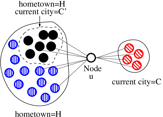
One standard method of label inference is label propagation (Zhu & Ghahramani, 2002; Zhu et al., 2003), which tries to set the label probabilities of nodes so that friends have similar probabilities. While this method succinctly captures the essence of homophily (the more two nodes have in common, the more likely they are to connect (McPherson et al., 2001)), it optimizes for only a single type of label and assumes only a single category of relationships. It therefore fails to address the potential complexity of edge formation in networks, where nodes have different reasons to link to each other. As an example, consider the snapshot of a social network in Figure 1, where we want to predict the hometown and current city of node , given what we know about and ’s neighbors. Here, the labels of node are completely unknown, but her friends’ labels are completely known. Label propagation would treat each label independently and infer the hometown of to be the most common hometown among her friends, the current city to be the most common current city among friends, and so on. Hence, if the bulk of friends of are from her hometown , then inferences for current city will be dominated by the most common current city among her hometown friends (say, ) and not friends from her actual current city ; indeed, the same will happen for all other label types as well.
Our proposed method, named EdgeExplain, approaches the problem from a different viewpoint, using the following intuition: Two nodes form an edge for a reason that is likely to be related to them sharing the value of one or more label types (e.g., two users went to the same college). Using this intuition, we can go beyond standard label propagation in the following way: instead of taking the graph as given, and modeling labels as items that propagate over this graph, we consider the labels as factors that can explain the observed graph structure. For example, the inferences for made by label propagation leave ’s edges from completely unexplained. Our proposed method rectifies this, by trying to infer node labels such that for each edge , we can point to a reason why this is so — and are friends from the same hometown, or college, or the like. While we are primarily interested in inferring labels, we note that the inferred reason for each edge can be important applications by itself; e.g., if a new node joins a network and forms and edge with , knowledge of the reason can help with the well-known link prediction task — should we recommend ’s college friends, or friends from the same high school, etc.?
We note that a seemingly simple alternative solution — cluster the graph and then propagate the most common labels within a cluster — is in fact quite problematic. In addition to the computation cost, any clustering based solely on the graph structure ignores labels already available from user profiles, but any clustering that tries to use these labels must deal with incomplete and missing labels. The clustering must also be complex enough to allow many overlapping clusters. Hence, we believe that clustering does not readily lend itself to a solution for our problem.
Our contributions are:
- 1.
We formulate the label inference problem as one of explaining the graph structure using the labels. We explicitly account for the fact that labels belong to a limited set of label types, whose properties we enumerate and incorporate into our model.
- 2.
Our gradient-based iterative method for inferring labels is easily implemented in large-scale message-passing architectures. We empirically demonstrate its scalability on a billion-node subset of the Facebook social network, using publicly available user profiles and friendships.
- 3.
On this large real-world dataset, EdgeExplain significantly outperforms label propagation for several label types, with lifts of up to for recall@1 and for recall@3. These improvements in accuracy, combined with the scalability of EdgeExplain, clearly demonstrate its usefulness for label inference on large networks.
The paper is organized as follows. We survey related work in Section 2. Our proposed model is discussed in Section 3, followed by the inference method in Section 4, and generalizations of the model in Section 5. Empirical evidence proving the effectiveness of our method is presented in Section 6, followed by conclusions in Section 7.
2 Related Work
We discuss prior work in semi-supervised learning, statistical relational learning, and in latent models for networks.
Semi-supervised learning. Many graph-based approaches can be viewed as estimating a function over the nodes of the graph, with the function being close to the observed labels, and smooth (similar) at adjacent nodes. Label propagation (Zhu et al., 2003; Zhu & Ghahramani, 2002) uses a quadratic function, but other penalties are also possible (Zhou et al., 2004; Belkin et al., 2004; Belkin et al., 2005). Other approaches modify the random walk interpretation of label propagation (Baluja et al., 2008; Talukdar & Crammer, 2009). In order to handle a large number of distinct label values, the label assignments can be summarized using count-min sketches (Talukdar & Cohen, 2014). None of the approaches consider interactions between multiple label types, and hence fail to capture the edge formation process in graphs considered here.
Statistical relational learning. These algorithms typically predict a label based on (a) a local classifier that uses a node’s attributes alone, (b) a relational classifier that uses the labels at adjacent nodes, and (c) a collective inference procedure that propagates the information through the network (Chakrabarti et al., 1998; Perlich & Provost, 2003; Lu & Getoor, 2003; Macskassy & Provost, 2007). Macskassy et al. (2007) observe that the best algorithms (weighted-vote relational neighbor classifier (Macskassy & Provost, 2007) with relaxation labeling (Rosenfeld & Hummel, 1976; Hummel & Zucker, 1983)) tend to perform as well as label propagation, which we outperform. While there has been some work focusing on understanding how to combine and weigh different edge types for best prediction performance (Macskassy, 2007), the edge types (analogous to our reason for an edge) were given up front. We note that these algorithms typically focus on a single label type, while we explicitly model the interactions among multiple types.
There is also extensive work on probabilistic relational models, including Relational Bayesian Networks (Koller & Pfeffer, 1998; Friedman et al., 1999), Relational Dependency Networks (Neville & Jensen, 2007), and Relational Markov Networks (Taskar et al., 2002). These are very general formalisms, but it is our explicit modeling assumptions regarding multiple label types that yields gains in accuracy.
Latent models. Graph structure has been modeled using latent variables (Hoff et al., 2002; Miller et al., 2009; Palla et al., 2012), but with an emphasis on link prediction. However, our goal is to make predictions about each individual user, and such latent features can be arbitrary combinations of user attributes, rather than concrete label types we wish to predict. Other models simultaneously explain the connections between documents as well as their word distributions (Nallapati et al., 2008; Chang & Blei, 2010; Ho et al., 2012). While we do not consider the problem of modeling text data, our model permits us to incorporate node attributes, such as group memberships. Finally, the number of distinct label values in our application is very large (on the order of millions), and we suspect that the latent variables would have to have a large dimension to explain the edges in our graph well.
3 Proposed Model
In this section we first build intuition about our model using a running example. Suppose we want to infer the labels (e.g., “Palo Alto High School” and “Stanford University”) corresponding to several label types (e.g., high school and college) for a large collection of users. The available data consist of labels publicly declared by some users, and the (public) social network among users, as defined by their friendship network. While the desired set of label types may depend on the application, here we focus on five label types: hometown, high school, college, current city, and employer.
Our solution exploits three properties of these label types:
- (P1)
They represent the primary situations where two people can meet and become friends, for example, because they went to the same high school or college.
- (P2)
These situations are (mostly) mutually exclusive. While there may be occasional friendships sharing, say, hometown and high-school, we make the simplifying assumption that most edges can be explained by only one label type.
- (P3)
Sharing the same label is a necessary but not sufficient condition. For example, “We are friends from Chicago” typically implies that the indicated individuals were, at some point in time, co-located in a small area within Chicago (say, lived in the same building, met in the same cafe), but hardly implies that two randomly chosen individuals from Chicago are likely to be friends.
(P1) is a direct result of our application; our desired label types were targeted at friendship formation. Combined with (P2), our five label types can be considered a set of mutually exclusive and exhaustive “reasons” for friendship; while this is not strictly true for high school and hometown, empirical evidence suggests that it is a good approximation (shown later in Section 6) and we defer a discussion on this point to Section 5. However, as (P3) shows, we cannot simply cast the labels as features whose mere presence or absence significantly affects the probability of friendship; instead, a more careful analysis is called for.
Formally, we are given a graph, and a set of label types . For each label type , let denote the (high-dimensional) set of labels for that label type. Each node in the graph is associated with binary variables , where if node has label for label type . Let and represent the sets of visible and hidden variables, respectively. We want to infer the correct values of , leveraging and .
A popular method for label inference is label propagation (Zhu & Ghahramani, 2002; Zhu et al., 2003). For a single label type, this approach represents the labeling by a set of indicator variables , where if node is labeled as and 0 otherwise. Zhu et al. (2003) relax the labeling to real-valued variables over all nodes and labels that are clamped to one (or zero) for nodes known to possess that label (or not). They then define a quadratic energy function that assigns lower energy states to configurations where at adjacent nodes are similar:
| (1) |
Here, means that and are linked by an edge, and is a non-negative weight on the edge . The minimum of Eq. 1 is found by solving the fixed point equations
| (2) |
where . This procedure encourages of nodes connected to clamped nodes to be close to the clamped value and propagates the labels outwards to the rest of the graph. Multiple label types can be handled similarly by minimizing Eq. 1 independently for each type.
While this formulation makes full use of (P1) and has the advantage of simplicity, it completely ignores (P2). Intuitively, label propagation assumes that friends tend to be similar in all respects (i.e., all label types), whereas what (P2) suggests is that each friendship tends to have a single reason: an edge exists because and share the same high school or college or current city, etc. This highly non-linear function is not easily expressed as a quadratic or similar variant.
Instead, we propose a different probabilistic model, which we call EdgeExplain. As described above, let and represent the sets of visible and hidden variables respectively; the variable is known (visible) if user has publicly declared the label for type , and unknown (hidden) otherwise. Then, EdgeExplain is defined as follows:
| (3) | ||||
| (4) | ||||
| (5) |
where is a normalization constant. Here, indicates whether a shared label type is the reason underlying the edge (Eq. 4). The function should have three properties: (a) it should be monotonically non-decreasing in each argument, (b) it should achieve a value close to its maximum as long as any one of its parameters is “high”, and also (c) it should be differentiable, for ease of analysis. In Eq. 5, we use the sigmoid function to implement this: . This monotonically increases from to , and achieves values greater than once is greater than an -dependent threshold. In addition, the sigmoid enables fine control of the degree of “explanation” required for each edge (discussed below) and allows for easy extensions to more complex label types and extra features (Section 5), all of which make it our preferred choice for the softmax.
In a nutshell, our modeling assumption can be stated as follows: It is better to explain as many friendships as possible, rather than to explain a few friendships really well. Eq. 3 is maximized if the softmax function achieves a high value for each edge , i.e., if each edge is “explained”. This is achieved if the sum is more than the required threshold, which in turn is satisfied if the product is 1 for even one label — in other words, when there exists any label that both and share. The parameter controls the degree of explanation needed for each edge; a small forces the learning algorithm to be very sure that and share one or more label types, while with a large , a single matching label type is enough. Empirical results shown later in Section 6 prove that large values perform better, suggesting that even a single matching label type is enough to explain the edge. The parameter in Eq. 5 can be thought of as the probability of matching on an unknown label type, distinct from the five we consider. Higher values of can be used to model uncertainty that the available label types form an exhaustive set of reasons for friendships. All our experiments use , and reflect our belief in property (P1); the accuracy of predictions under this setting (shown later in Section 6) suggests that (P1) indeed holds true.
Further intuition can be gained by considering a node whose labels are completely unknown, but whose friends’ labels are completely known (see Figure 1). As we discussed earlier in Section 1, label propagation would infer the hometown of to be the most common hometown among her friends (i.e., ), the current city to be the most common current city among friends (i.e., ), and so on. However, such an inference leaves ’s friendships from completely unexplained. Our proposed method rectifies this; Eq. 3 will be maximized by correctly inferring and as ’s hometown and current city respectively, since is enough to explain all friendships with the hometown friends, and the marginal extra benefit obtained from explaining these same friendships a little better by using as ’s current city is outweighed by the significant benefits obtained from explaining all the friendships from by setting ’s current city to be .
To summarize, Eq. 4 encapsulates property (P1) by trying to have matching labels between friends; Eq. 5 models property (P2) by enabling any one label type to explain each friendship; and the form of the probability distribution (Eq. 3) uses only existing edges and not all node pairs, and thus is not affected when, say, two nodes with Chicago as their current city are not friends, which reflects the idea that matching label types are necessary but not sufficient (P3).
4 Inference
The probabilistic description of EdgeExplain in Eqs. 3-5 can be restated as an optimization problem in the variables . In the spirit of (Zhu et al., 2003), we propose a relaxation in terms of a real-valued function , with representing the probability that , i.e., the probability that user has label for label type . This yields the following optimization:
| Maximize | (6) | |||
| (7) | ||||
| (8) | ||||
| (9) |
where is defined as in Eq. 5, and the equation for is analogous to Eq. 4 but measures the total probability that and have the same label for a given label type .
The problem is not convex in , but is convex in if the distributions are held fixed for all nodes . Hence, we propose an iterative algorithm to infer . Given for all , finding the optimal corresponds to solving the following problem:
where the summation is only over the set of the friends of , and we again restrict to be a set of probability distributions, one for each label type. We note that is convex and Lipschitz continuous with constant , where is the number of friends of .
This is a constrained maximization problem with no closed form solution for . To solve it, we use proximal gradient ascent, which is an iterative method where in each step, we take a step in the direction of the gradient, and then project it back to the probability simplex . Specifically, let represent the gradient of , with components given by:
Let be the estimated probability distributions for each of the label types at the end of iteration , and let represent the (possibly improper) ending point of the -th gradient step:
where is a step-size parameter that we could set to a constant . The point is now projected to the closest point in :
This can be easily achieved in expected linear time over the size of the label set (Duchi et al., 2008). If only sparse distributions can be stored for each label type (say, only the top labels for each type), the optimal -sparse projections can be obtained simply by setting to all but the top labels for each label type, and then projecting on to the simplex (Kyrillidis et al., 2013).
This algorithm converges to a fixed point, and the function values converge to the optimal at a rate (Beck & Teboulle, 2009):
where represents the optimal set of probability distributions, and is the optimal function value. An important consequence of the algorithm is that computation of only requires information from for the neighbors of . Thus, it is a “local” algorithm that can be easily implemented in distributed message-passing architectures, such as Giraph (Giraph, ; Ching, 2013).
5 Generalizations
We now discuss some aspects of EdgeExplain and some generalizations that demonstrate its wide applicability.
Related label types. Property (P2) assumes that the reasons for friendship formation are mutually exclusive, but this need not be strictly true. For example, some high school friends could be a subset of hometown friends11 1 The relationship between high school and hometown is in fact more complicated. The high school could be within driving distance of the hometown, but not in it; and sometimes even this does not hold.. Let us again consider Figure 1, but with current city replaced by high school. Suppose that the solid-black nodes represent actual high school friends, and we are trying to infer ’s high school. If the small cluster on the right did not exist, then Eq. 3 would be maximized by picking the most common high school among ’s friends (i.e., the solid-black nodes), even if they are already explained by a shared hometown; thus, EdgeExplain would pick the correct high school. On the other hand, if some friendships would remain unexplained without a shared high school (e.g., the small cluster in Figure 1), then it is not obvious whether we should prefer a high school that explains these edges or a high school that represents a large segment of hometown friends. The parameter modulates this trade-off, with a higher value of emphasizing the explanation of all edges as against the explanation of several edges a little better. The choice of must depend on the characteristics of the social network; for the Facebook network, the best empirical results are achieved for large (shown later in Section 6), suggesting that many of our label types are indeed mutually exclusive.
Incorporating user features. EdgeExplain easily generalizes to broader settings with multiple user features, such as group memberships, topics of interest, keywords, or pages liked by the user. As an example, consider group memberships of users. Intuitively, if most members of a group come from the same college, then it is likely a college-friends group, and this can aid inference for group members whose college is unknown. This can be easily handled by creating a special node for each group, and creating “friendship” edges between the group node and its members. EdgeExplain will infer labels for the group node as well, and will explain its “friendships” via the college label. This, in turn, will influence college inference for group members with unknown college labels. The importance of such group membership features can also be tuned, as described next.
Incorporating edge features. There are several situations where edge-specific features could be useful. First, we may want to give more importance to certain kinds of edges, such as the group-membership edges mentioned above. Second, some features could be important for one label type but not another: e.g., the age difference between friends could be useful for inferring high school but not employer. All these situations can be easily handled by modifying Eq. 4 to include an edge-specific and label type-specific weight. The corresponding modifications to the inference method are trivial.
6 Experiments
Previously, we provided intuition and examples supporting the claim that EdgeExplain is better suited to inference of our desired label types than vanilla label propagation. In this section, we demonstrate this via empirical evidence on a billion-node graph.
Data. We ran experiments on a large subgraph of the Facebook social network, consisting of over billion users and their friendship edges. From the public profile of each user, we extract the hometown, current city, high school, college, and employer, whenever these are available. The dimensionality of our five label types range from almost to over . We describe below in Implementation Details our process for generating the edges. This forms our base dataset.
 |
 |
|---|---|
| (a) Recall at | (b) Recall at |
Experimental Methodology. The set of users is randomly split into five parts and experimental accuracy is measured via 5-fold cross-validation, with the known profile information from four folds being used to predict labels for all types for users in the fifth fold. Results over the various folds are identical to three decimal places. All differences are therefore significant and we do not show variances as they are too small to be noticeable.
In each experiment, we run inference on the training set and compute a ranking of labels for each label type for each user. This ranking is provided by computed for label propagation (Eq. 1) and EdgeExplain (Eqs. 6-9) respectively. We then measure recall at the top- and top- positions, i.e., we measure the fraction of (user, label type) pairs in the test set where the predicted top-ranked label (or any of the top- labels) match the actual user-provided label. For reasons of confidentiality, we only present the lift in recall values of EdgeExplain as compared to label propagation.
Implementation Details. We implemented EdgeExplain in Giraph (Giraph, ; Ching, 2013) which is an iterative graph processing system based on the Bulk Synchronous Processing model (Malewicz et al., 2010; Valiant, 1990). The entire set of nodes is split among machines, and in each iteration, every node sends the probability distributions to all friends of . To limit the communication overhead, we implemented two features: (a) for each user and label type , the multinomial distribution was clipped to retain only the top entries optimally (Kyrillidis et al., 2013), and (b) the friendship graph is sparsified so as to retain, for each user , the top friends whose ages are closest to that of . This choice of friends is guided by the intuition that friends of similar age are most likely to share certain label types such as high school and college. We find that clipping the distributions makes little difference to accuracy while significantly improving running time. However, the value of matters significantly, and we detail these effects next.
Recall of EdgeExplain. Figure 2 shows recall as a function of varying number of friends , against a baseline of EdgeExplain with . We observe that recall increases up to a certain and then decreases — for recall at , and for recall at . This demonstrates both the importance and the limits of scalability: increasing the number of friends enables better inference but beyond a point, more friends increase noise. Thus, friends appear to be enough for inference under EdgeExplain.
Figure 2 also shows an increasing trend from hometown to employer in the degree of improvement obtained over the baseline. This is because (a) the baseline itself is best for hometown and worst for employer, but also because (b) Facebook users appear to have many more friends from label types other than from their current employer. The effect of this latter observation is that if we only have a small , it is very likely that the few friends from the same current employer are not included in that limited set of friends (which we empirically verified). As increases and such same-employer edges become available, EdgeExplain can easily learn the reason for these edges (hence the dramatic increase in recall), but label propagation will likely be confused by the overall distribution of different employers among all friends and therefore does not benefit equally from adding more friends, as we show next.
 |
 |
| (a) Recall at | (b) Recall at |
Comparison with Label Propagation. Figure 3 shows the lift in recall achieved by EdgeExplain over Label Propagation as we increase for both. We observe similar performance of both methods for hometown and current city, but increasing improvements for high school, college, and employer. This again points to the first two being easier to infer, with the difficulty of inference increase with the latter label types. With fewer employer-based friendships, the prototypical example of Figure 1 would also occur frequently, with Label Propagation likely picking common employers of (say) hometown friends instead of the less common friendships based on the actual employer. By attempting to explain each friendship, EdgeExplain is able to infer the employer even under such difficult circumstances, and the ability to perform well even for under-represented label types makes EdgeExplain particularly attractive.
| Label Type | Recall at | Recall at |
|---|---|---|
| Hometown | ||
| Current city | ||
| High school | ||
| College | ||
| Employer |
Inclusion of extra features. In Section 5, we discussed how extra features could be used within the EdgeExplain framework. In particular, we showed how the fact that some users are members of groups can be used to infer (say) their college, if the group turns out to be college-specific group. Group memberships are extensive and provide information that is orthogonal to friendships; thus, a priori, one would expect the addition of group membership features to have significant impact on label inference.
Table 1 shows the lift in recall for EdgeExplain when group memberships are used in addition to friends. While the addition of group memberships increases the size of the graph by , the observed benefits for recall are minor: a maximum lift of only for employer inference, and indeed reduced recall at for several label types. Note that the lift in recall would have appeared very significant had we compared it to Label Propagation with ; however, this gain largely disappears when the friendships are considered in the framework of EdgeExplain. Thus, it is not merely the scalability of EdgeExplain, but also the careful modeling of properties (P1)-(P3) that makes group membership redundant.
Given the a priori expectations of the impact of group memberships, this surprising result suggests that information regarding our label types are already encoded in the structure of the social network and hence the orthogonal information from the group memberships actually turn out to be redundant.

The limits of resolution. Our model theoretically should be able to handle any number of label types, but empirically this may not hold true for our network. How many friends sharing a certain label type (say, the same college) does a user need to have in order to correctly infer the value of that label type? To answer this, we select, for each user, the set of friends whose label for the given label type is known, and we compute the fraction that actually shared the user’s label for . Figure 4 shows the probability that EdgeExplain correctly infers the user’s label as a function of this fraction (i.e., the correct label is among the top 3 predictions). All label types are similar, though high school is somewhat easier and employer harder; having of friends sharing a user’s label is sufficient to infer the label in our graph. Note that certain label types are more likely to be publicly declared than others, and this explains differences in recall observed earlier.

Effect of . Figure 5 shows that the lift in recall at for various values of the parameter , with respect to . Performance generally improves with increasing . Results for recall at are qualitatively similar, though the effect is more muted. We find that offer the best results, and EdgeExplain is robust to the specific choice of within this range. Recall that with large , a single matching label is enough to explain an edge, while with small , multiple matching labels may be needed. Thus, the outperformance of large provides strong empirical validation of property (P2) (on our network).

Running time. Figure 6 shows the wall-clock time as a function of . The running time should depend linearly on the graph size, which grows almost linearly with ; as expected, the plot is linear, with deviations due to garbage collection stoppages in Java.
7 Conclusions
We proposed the problem of jointly inferring multiple correlated label types in a large network and described the problems with existing single-label models. We noted that one particular failure mode of existing methods in our problem setting is that edges are often created for a reason associated with a particular label type (e.g., in a social network, two users may link because they went to the same high school, but they did not go to the same college). We identified three network properties that model this phenomenon: edges are created for a reason (P1), they are generally created only for one reason (P2), and sharing the same value for a label type is necessary but not sufficient for having an edge between two nodes (P3).
We introduced EdgeExplain, which carefully models these properties. It leverages a gradient-based method for collective inference which allows for fast iterative inference that is equivalent in running time to basic label propagation. Our experiments with a billion-node subset of the Facebook graph amply demonstrate the benefits of EdgeExplain, with significant improvements across a set of different label types. Our further analysis validates many of the properties and intuitions we had about modeling networks, primarily that one can achieve significant improvements if one considers and models the reason an edge exists. Whether one is interested in inferring one or multiple label types, modeling these explanations will have significant impact on the accuracy of the final predictions.
References
- Baluja et al. (2008) Baluja, S., Seth, R., Sivakumar, D., Jing, Y., Yagnik, J., Kumar, S., Ravichandran, D., and Aly, M. Video suggestion and discovery for YouTube: Taking random walks through the view graph. In WWW, pp. 895–904, 2008.
- Beck & Teboulle (2009) Beck, A. and Teboulle, M. Gradient-based algorithms with applications to signal recovery. 2009.
- Belkin et al. (2004) Belkin, M., Matveeva, I., and Niyogi, P. Tikhonov regularization and semi-supervised learning on large graphs. In COLT, pp. 624–638, 2004.
- Belkin et al. (2005) Belkin, M., Niyogi, P., and Sindhwani, V. On manifold regularization. In AISTATS, 2005.
- Chakrabarti et al. (1998) Chakrabarti, S., Dom, B., and Indyk, P. Enhanced hypertext categorization using hyperlinks. In SIGMOD, volume 1, pp. 307–319, 1998.
- Chang & Blei (2010) Chang, J. and Blei, D. Hierarchical relational models for document networks. The Annals of Applied Statistics, 4(1):124–150, September 2010.
- Ching (2013) Ching, A. Scaling Apache Giraph to a trillion edges. Facebook Engineering blog, 2013.
- Duchi et al. (2008) Duchi, J., Shalev-Shwartz, S., Singer, Y., and Chandra, T. Efficient projections onto the -ball for learning in high dimensions. In ICML, 2008.
- Friedman et al. (1999) Friedman, N., Getoor, L., Koller, D., and Pfeffer, A. Learning Probabilistic Relational Models. In IJCAI, pp. 1300–1309, 1999.
- (10) Giraph. The Apache Giraph Project. http://giraph.apache.org.
- Ho et al. (2012) Ho, Q., Eisenstein, J., and Xing, E. Document hierarchies from text and links. In WWW, pp. 739–748, 2012.
- Hoff et al. (2002) Hoff, P., Raftery, A., and Handcock, M. Latent space approaches to social network analysis. JASA, 97(460):1090–1098, 2002.
- Hummel & Zucker (1983) Hummel, R. and Zucker, S. On the foundations of relaxation labeling processes. IEEE PAMI, 5:267–287, 1983.
- Koller & Pfeffer (1998) Koller, D. and Pfeffer, A. Probabilistic frame-based systems. In AAAI, pp. 580–587, 1998.
- Kyrillidis et al. (2013) Kyrillidis, A., Becker, S., Cevher, V., and Koch, C. Sparse projections onto the simplex. JMLR, 28(2), 2013.
- Lu & Getoor (2003) Lu, Q. and Getoor, L. Link-based classification. In ICML, 2003.
- Macskassy (2007) Macskassy, S. A. Improving learning in networked data by combining explicit and mined links. In AAAI, 2007.
- Macskassy & Provost (2007) Macskassy, S. A. and Provost, F. Classification in networked data: A toolkit and a univariate case study. JMLR, 8:935–983, 2007.
- Malewicz et al. (2010) Malewicz, G., Austern, M. H., Bik, A. J. C., Horn, I., Leiser, N., and Czajkowski, G. Pregel: A system for large-scale graph processing. In SIGMOD, 2010.
- McPherson et al. (2001) McPherson, M., Smith-Lovin, L., and Cook, J. M. Birds of a Feather: Homophily in Social Networks. Annual Review of Sociology, 27:415–444, 2001.
- Miller et al. (2009) Miller, K., Griffiths, T., and Jordan, M. Nonparametric latent feature models for link prediction. In NIPS, pp. 1276–1284, 2009.
- Nallapati et al. (2008) Nallapati, R., Ahmed, A., Xing, E., and Cohen, W. Joint latent topic models for text and citations. In KDD, pp. 542, 2008.
- Neville & Jensen (2007) Neville, J. and Jensen, D. Relational Dependency Networks. JMLR, 8:653–692, 2007.
- Palla et al. (2012) Palla, K., Knowles, D., and Ghahramani, Z. An infinite latent attribute model for network data. In ICML, 2012.
- Perlich & Provost (2003) Perlich, C. and Provost, F. Aggregation-based feature invention and relational concept classes. In KDD, pp. 167, 2003.
- Rosenfeld & Hummel (1976) Rosenfeld, A. and Hummel, R. Scene labeling by relaxation operations. KDD, SMC-6(6):420–433, 1976.
- Talukdar & Cohen (2014) Talukdar, P. and Cohen, W. Scaling graph-based semi supervised learning to large number of labels using count-min sketch. In AISTATS, 2014.
- Talukdar & Crammer (2009) Talukdar, P. and Crammer, K. New regularized algorithms for transductive learning. In ECML, 2009.
- Taskar et al. (2002) Taskar, B., Abbeel, P., and Koller, D. Discriminative Probabilistic Models for Relational Data. In UAI, pp. 485–492, 2002.
- Valiant (1990) Valiant, L. G. A bridging model for parallel computation. CACM, 33(8), 1990.
- Zhou et al. (2004) Zhou, D., Bousquet, O., Lal, T., Weston, J., and Schölkopf, B. Learning with local and global consistency. In NIPS, volume 1, 2004.
- Zhu & Ghahramani (2002) Zhu, X. and Ghahramani, Z. Learning from labeled and unlabeled data with label propagation. Technical report, Carnegie Mellon University, 2002.
- Zhu et al. (2003) Zhu, X., Ghahramani, Z., and Lafferty, J. Semi-supervised learning using Gaussian fields and harmonic functions. In ICML, 2003.