Generalized second law of thermodynamics in scalar-tensor gravity
Abstract
Abstract
Within the
context of scalar-tensor gravity, we explore the generalized second
law (GSL) of gravitational thermodynamics. We extend the action of
ordinary scalar-tensor gravity theory to the case in which there is
a non-minimal coupling between the scalar field and the matter field
(as chameleon field). Then, we derive the field equations governing
the gravity and the scalar field. For a FRW universe filled only
with ordinary matter, we obtain the modified Friedmann equations as
well as the evolution equation of the scalar field. Furthermore, we
assume the boundary of the universe to be enclosed by the dynamical
apparent horizon which is in thermal equilibrium with the Hawking
temperature. We obtain a general expression for the GSL of
thermodynamics in the scalar-tensor gravity model. For some viable
scalar-tensor models, we first obtain the evolutionary behaviors of
the matter density, the scale factor, the Hubble parameter, the
scalar field, the deceleration parameter as well as the effective
equation of state (EoS) parameter. We conclude that in most of the
models, the deceleration parameter approaches a de Sitter regime at
late times, as expected. Also the effective EoS parameter acts like
the CDM model at late times. Finally, we examine the
validity of the GSL for the selected
models.
PACS numbers: 04.50.Kd
Keywords: Modified theories of gravity
Keywords:
Modified theories of gravity; Dark energypacs
04.50.KdI Introduction
During the last decade, observational cosmology has entered an era of unprecedented precision. Measurements of the cosmic microwave background (CMB) ([1, 2]), the Hubble constant () [3], the luminosity and distance at high redshift with supernovae Ia [4], and baryon acoustic oscillations (BAO) surveys [5], suggest that our Universe is currently undergoing a phase of accelerated expansion. The proposals that have been put forth to explain these interesting discoveries can basically be classified into two categories. One is to assume the cosmic speed-up might be caused within general relativity (GR) by a mysterious cosmic fluid with negative pressure, which is usually called dark energy (DE). However, the nature of DE is still unknown and the problem of DE is one of the hardest and unresolved problems in modern theoretical physics (see [6, 7] and references therein).
Alternatively, the acceleration could be due to purely gravitational effects, named modified gravity, i.e., one may consider modifying the current gravitational theory to produce an effective DE. One such modification is referred to as -gravity, in which the Einstein-Hilbert action in GR is generalized from the Ricci scalar to an arbitrary function of the Ricci scalar (for a good review see [8] and references therein). There are also some other classes of modified gravities containing [9], [10] and [11] which are considered as gravitational alternatives for DE. Here, is the Gauss-Bonnet invariant term. Also and are the Riemann and Ricci tensors, respectively, and is the torsion scalar. The modified gravity can unify the early-time inflation with late-time acceleration without resorting to the DE [8]. Moreover, modified gravity may serve as dark matter (DM) [12].
In the context of modified gravity, there is also a large class of models called scalar-tensor theories [13, 14], which take into account the effects due to the non-minimal coupling term between a scalar field and a Ricci scalar curvature. In scalar-tensor theories, if the evolution of matter perturbations is known observationally, together with the Hubble parameter , one can even determine the function together with the potential of the scalar field [15]. Scalar-tensor theories also contains a class of models called chameleon gravity [16, 17, 18] in which there is a non-minimal coupling between the scalar field and the matter field. Historically, one of the first scalar-tensor theories is the Brans-Dicke theory of gravity which has been motivated from Mach’s principle. This is achieved in Brans-Dicke theory by making the effective gravitational coupling strength depend on the space-time position and being governed by distant matter sources. Modern interest in Brans-Dicke and scalar-tensor theories is motivated by the fact that they are obtained as low-energy limits of string theories. It was shown that metric and Palatini (but not metric-affine) modified gravities can be reduced to scalar-tensor theories [19].
Thermodynamics of the accelerating universe driven by the DE or dark gravity (due to the modified gravity effect) is one of interesting issues in modern cosmology. In the context of black hole thermodynamics, Jacobson using the first law of thermodynamics on the local Rindler horizons and assuming the Bekenstein-Hawking entropy-area relation , where is the area of the horizon and is Newton’s constant, was able to derive the Einstein equations [20]. The study on the connection between gravity and thermodynamics has been extended to cosmological context. It was pointed out that the Friedmann equation in the Einstein gravity can be obtained using the first law of thermodynamics (Clausius relation) on the apparent horizon with the Hawking temperature and Bekenstein-Hawking entropy [21]. The relation between gravity and thermodynamics has been further disclosed in extended gravitational theories, including the theory [21], scalar-tensor gravity and -gravity [22], Lovelock theory [23] and braneworld scenarios (such as DGP, RSI and RSII) [24].
Note that the entropy-area relation familiar from GR is still valid in the other modified gravity theories provided that Newton’s constant is replaced by a suitable effective gravitational coupling strength . For instance, the effective Newton’s constant in -gravity and -gravity are given by [25] and [26], respectively, where prime denotes a derivative with respect to the Ricci and torsion scalars. In scalar-tensor gravity, the geometric entropy is also given by [19, 27] with [19, 27].
In addition to the first law of thermodynamics, the generalized second law (GSL) of gravitational thermodynamics, which states that entropy of the fluid inside the horizon plus the geometric entropy do not decrease with time, has been studied extensively in the literature [28]-[37]. The GSL of thermodynamics like the first law is a universal principle governing the Universe. Here, our aim is to investigate the GSL of thermodynamics in the framework of scalar-tensor gravity. As one of the most important theoretical touch stones to examine whether scalar-tensor gravity can be an alternative gravitational theory to GR, we explore the GSL of thermodynamics in scalar-tensor gravity, and derive the condition for the GSL to be satisfied. The paper is organized as follows. In section II we investigate the scalar-tensor gravity and extend it to the case in which there is a non-minimal coupling between the scalar field and the matter field (as chameleon field). In section III, we explore the GSL of thermodynamics on the dynamical apparent horizon of a Friedmann-Robertson-Walker (FRW) universe filled with the ordinary matter which is in thermal equilibrium with the Hawking temperature. In sections IV-VIII, we examine the validity of the GSL for some viable scalar-tensor gravity models containing Brans-Dicke gravity, Brans-Dicke gravity with a self interacting potential, chameleon gravity, chameleonic generalized Brans-Dicke gravity and chameleonic Brans-Dicke gravity with a self interacting potential. Section IX is devoted to conclusions.
II Scalar-tensor gravity
In the Jordan frame, general action of the scalar-tensor gravity can be written as
| (1) |
where . Also , , and are the determinant of metric , the Ricci scalar curvature, the scalar field and the matter Lagrangian, respectively. Also , and are arbitrary dimensionless functions, and is the scalar field potential. Note that in action (1), the terms and show that the scalar field is nonminimally coupled to the scalar curvature (as Brans-Dicke field with ) and the matter Lagrangian (as chameleon field), respectively. In the absence of chameleon field, i.e. , Eq. (1) reduces to the ordinary action of the scalar-tensor gravity theory [38].
Taking variations of the action (1) with respect to and lead to the corresponding field equations in scalar-tensor gravity as
| (2) |
| (3) |
where is the Einstein tensor, is the Ricci tensor and is the energy-momentum tensor of the matter fields. Also is the covariant derivative associated with and the subscript denotes a derivative with respect to the scalar field (i.e. ). We assume that has the form of the energy-momentum tensor of a perfect fluid
| (4) |
Now we consider a spatially non-flat universe described by the FRW metric
| (5) |
where represent a flat, closed and open universe, respectively. Substituting the FRW metric (5) into the field equations (2) yields the Friedmann equations in scalar-tensor gravity as
| (6) |
| (7) |
Also Eq. (3) for the FRW metric (5) gives the equation governing the evolution of the scalar field as
| (8) |
where
| (9) |
and is the Hubble parameter. Here the dot denotes a derivative with respect to cosmic time . Note that in the absence of chameleon field, i.e. , Eqs. (6), (7) and (8) are same as those obtained for the ordinary scalar-tensor gravity [38].
The Friedmann equations (6) and (7) can be rewritten in the standard form as
| (10) |
| (11) |
where and are the effective (total) energy density and pressure defined as
| (12) | |||
| (13) |
Here and are the energy density and pressure due to the scalar field contribution defined as
| (14) |
| (15) |
Note that the scalar field contributions and in scalar-tensor gravity can justify the observed acceleration of the universe without resorting to the DE. For a special case , from Eqs. (14) and (15) we have and , then Eqs. (10) and (11) transform to the usual Friedmann equations in the Einstein gravity.
The energy conservation laws in scalar-tensor gravity can be obtained as
| (16) |
| (17) |
Also and satisfy the following energy equation
| (18) |
Note that the set of equations containing the Friedmann equations (6) and (7), the evolution equation of the scalar field (8) and the continuity equation governing the matter field (16) are not independent of each other. Taking the time derivative of Eq. (6) and using Eqs. (8) and (16), one can get the second Friedmann equation (7). In the next sections, we take the set of Eqs. (7), (8) and (16) which can uniquely determine the dynamics of the Universe.
III GSL in scalar-tensor gravity
Here in the context of scalar-tensor gravity theory, we explore the GSL of gravitational thermodynamics on the dynamical apparent horizon of a FRW universe filled only with ordinary matter which is in thermal equilibrium with the Hawking temperature. The GSL states that the sum of entropy of fluid filling the universe along with the entropy of the cosmological horizon must be increasing (or non-decreasing) function of time [21].
For a spatially non-flat FRW universe, the dynamical apparent horizon takes the form [39]
| (19) |
which in the case of flat universe (), it reduces to the Hubble horizon, i.e. . On the apparent horizon, the associated Hawking temperature is defined as [21]
| (20) |
where the condition is necessary due to having a positive temperature. Cai et al. [40] using the tunneling approach, proved that there is indeed a Hawking radiation with temperature (20), for a locally defined apparent horizon of a FRW universe with any spatial curvature.
The entropy of the matter inside the horizon satisfies the Gibbs equation [28]
| (21) |
where and is the volume of the dynamical apparent horizon containing the matter. Here, we have assumed the local equilibrium hypothesis to hold [41, 42].
Taking the time derivative of Eq. (21) and using (16) gets the equation governing the evolution of the matter entropy as
| (22) |
Using Eq. (7), this can be rewritten as
| (23) |
The geometric entropy in the scalar-tensor gravity is given by [27]
| (24) |
where is the area of the apparent horizon. Taking the time derivative of Eq. (24) and using (20) yields the evolution of the horizon entropy as
| (25) |
Now according to the GSL of gravitational thermodynamics, we can consider the entropy of the universe as the sum of the entropy of the matter inside the horizon, and the horizon entropy. Adding Eqs. (23) and (25) and using the auxiliary relation
| (26) |
the GSL in scalar-tensor gravity reads
| (27) |
where
| (28) |
| (29) |
| (30) |
and . Equation (27) shows that the validity of the GSL, i.e. , depends on the scalar-tensor gravity model. For instance, in the Einstein gravity, i.e. and , the GSL (27) yields
| (31) |
which shows that the GSL in Einstein’s gravity is always satisfied.
Here following [43], we try to rewrite the GSL (27) in terms of the effective equation of state (EoS) parameter defined as
| (32) |
where we have used Eqs. (10) and (11). From Eqs. (19), (26) and (32) one can get
| (33) |
Replacing this into Eqs. (22) and (25) yield
| (34) |
| (35) |
where is the EoS parameter of the ordinary matter. In the framework of Einstein gravity, i.e. and , for a flat FRW universe dominated by a single fluid () filling the volume enclosed by the apparent (Hubble) horizon () we have and Eq. (34) reduces to Eq. (11) in [43].
In the absence of chameleon scalar field, i.e. , Eq. (34) reduces to
| (36) |
Note that for the ordinary matter we have , hence the contribution of the matter entropy in the GSL will be positive or nil for and negative otherwise.
For a chameleon scalar field minimally coupled to the Ricci scalar curvature, i.e. , Eq. (35) yields
| (37) |
which shows that for the horizon entropy has a positive or nil contribution in the GSL.
Adding Eqs. (34) and (35) gives the GSL as
| (38) |
In the Einstein gravity, i.e. and , we have and and then the GSL (38) reduces to
| (39) |
which is always respected. This also can be obtained by replacing Eqs. (19) and (32) into (31).
Note that in general one cannot explore the validity of the GSL (38) in terms of , explicitly, even in some special cases like and . To do so, we need to solve the set of Eqs. (7), (8) and (16), numerically, for obtaining the evolutions of (or ), and .
In what follows, we are interested in examining the validity of GSL for some viable scalar-tensor gravity models. We further assume the Universe to be spatially flat, i.e. , which is compatible with the recent observations [1].
IV Model I: Brans-Dicke gravity
The action of Brans-Dicke (BD) theory is given by [44, 45]
| (40) |
where is the dimensionless BD parameter.
By comparing the actions (40) and (1) one can get
| (41) |
Substituting the above relations into Eqs. (8) and (16), for a flat universe one can obtain
| (42) |
| (43) |
Also the GSL (27) for a flat universe reduces to
| (44) |
where we take . Equation (43) for the pressureless matter (i.e. ) yields
| (45) |
Replacing Eqs. (41) and (45) into the second Friedmann equation (7) yields
| (46) |
To obtain the evolutionary behavior of the GSL (44), we first need to know the time evolution of both the Hubble parameter and the scalar field . To do so, one can obtain and by the numerical solving of Eqs. (42) and (46). Taking [2], [46] and using the initial values , , and [46], the variations of the scale factor, the Hubble parameter and the scalar field versus redshift are plotted in Figs. 1(a), 1(b) and 1(c), respectively. Also the evolutionary behaviors of the deceleration parameter,
| (47) |
and the effective EoS parameter , Eq. (32), in terms of redshift are plotted in Figs. 1(d) and 1(e), respectively.
Figures 1(a) to 1(e) show that: (i) the scale factor, the Hubble parameter and the scalar field, respectively, increases, decreases and increases during history of the Universe. (ii) The deceleration parameter shows a cosmic deceleration to acceleration transition in the near past which is compatible with the observations [47]. (iii) The effective EoS parameter at late times goes to which behaves like the quintessence model [48].
With the help of numerical results obtained for the Hubble parameter and the scalar field presented in Figs. 1(b) and 1(c), the variation of the GSL (44) versus is plotted in Fig. 1(f). The figure shows that the GSL in the BD gravity model (40) is satisfied during the late cosmological history of the Universe, i.e. .
V Model II: BD gravity with a self interacting potential
The action of BD theory with a self interacting potential and a matter field is given by [49]
| (48) |
with
| (49) |
Here and are two constants and is a positive integer.
By comparing the actions (48) and (1) we find
| (50) |
Inserting the above relations into Eqs. (8) and (16), for a flat universe one can obtain
| (51) |
| (52) |
where the evolution of for the pressureless matter () is same as that obtained in (45).
Inserting Eqs. (45) and (50) into the second Friedmann equation (7), one can find
| (54) |
which is same as Eq. (46) for the BD gravity model (40). Because the form of potential of the scalar field does not appear explicitly in the second Friedmann equation (7).
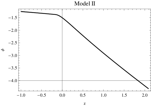
Taking [2] [46] and [49], the time evolution of both the scale factor and the scalar field can be obtained by numerical solving of Eqs. (51) and (54) with the initial values , , and . Also we set and to recast the differential Eqs. (51) and (54) in dimensionless form which is more suitable for numerical integration. The numerical results obtained for , , , and are plotted in Figs. 2(a), 2(b), 2(c), 2(d) and 2(e), respectively. Figures show that (i) , and , respectively, increases, decreases and increases during history of the Universe. (ii) The deceleration parameter shows a transition from the deceleration era to the acceleration regime . At late times (), the deceleration parameter approaches a de Sitter regime (i.e. ), as expected. (iii) The effective EoS parameter shows a transition from the quintessence state, , to the phantom regime, , in the future. Also at late times we get which acts like the CDM model.
The results of and illustrated in Figs. 2(b) and 2(c) help us to obtain the variation of the GSL (53) for the BD gravity model (48) with a self interacting potential (49). The result is plotted in Fig. 2(f). The figure shows that the GSL for our model is satisfied from the past to the present epoch. But in the future the GSL is violated for .
VI Model III: chameleon gravity
The action of chameleon gravity in the presence of matter is given by [50, 51]
| (55) |
where there is a non-minimal coupling term, , between the chameleon scalar field and the matter field.
Comparing the chameleon gravity action (55) with action (1), one can get
| (56) |
With the help of these relations, Eqs. (8) and (16) for a flat universe read
| (57) |
| (58) |
where we take . Taking the integration of Eq. (58) for the pressureless matter () gives
| (59) |
Substituting the relations (56) into (27) gives the GSL for a flat universe as
| (60) |
According to [51] we consider both and potential appeared in (55) behave exponentially as
| (61) |
where , , and are arbitrary constants.
Using Eqs. (59) and (61), the evolution Eq. (57) for the pressureless matter () gives
| (62) |
Also the second Friedmann equation (7) reads
| (63) |
Finally, the GSL (60) takes the form
| (64) |
From numerical solving of Eqs. (62) and (63) one can obtain and . To do so we take [2], and [51] and use the initial values , , and . The variations of , , , and versus redshift are plotted in Figs. 3(a) to 3(e). Figures show that (i) the scale factor increases when the time increases. The Hubble parameter decreases with increasing time and then increases to approach a constant value. The scalar field decreases with increasing time and increases at late times. (ii) The deceleration parameter shows a cosmic transition from to in the near past which is compatible with the observations [47]. It also approaches a de Sitter regime at late times, as expected. (iii) The effective EoS parameter can justify the transition from the quintessence state () to the phantom regime () in the near past, as indicated by recent observations [52]. This is also in good agreement with that obtained in [51]. The effective EoS parameter also behaves like the CDM model at late times.
With the help of numerical results obtained for the Hubble parameter and the scalar field illustrated in Figs. 3(b) and 3(c), the variation of the GSL (64) versus redshift for the chameleon gravity model is plotted in Fig. 3(f). The figure shows that the GSL in this model is violated for the range of . This is in contrast with that obtained in [51]. Authors of Ref. [51] investigated the GSL in flat FRW chameleon cosmology and showed that in an expanding universe, the GSL is always respected. This contradiction comes back to the definition of energy and pressure in the Gibbs equation (21). In [51], Farajollahi et al. considered effective (total) energy and pressure instead of and as we have in our case. Therefore in [51], the GSL is defined as in which
and is given by Eq. (37). Finally the GSL yields Eq. (39) which is nothing but the GSL in the Einstein gravity. This confirms that the GSL investigated in [51] does not belong to the chameleon gravity.
VII Model IV: chameleonic generalized BD gravity
Comparing Eq. (65) with action (1) gives
| (66) |
Using these, Eqs. (8) and (16) for a flat universe read
| (67) |
| (68) |
where . Solution of Eq. (68) for the pressureless matter () yields the same result obtained in (59).
With the help of relations (66), the GSL (27) for a flat universe yields
| (69) |
According to [46] we take
| (70) |
Substituting Eqs. (59) and (70) into (67) for the pressureless matter () gives
| (71) |
Also the second Friedmann equation (7) gives
| (72) |
Moreover the GSL (69) reduces to
| (73) |
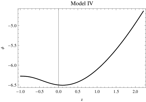
Taking [2], , and [46], the time evolution of both the scale factor and the scalar field can be obtained by numerical solving of Eqs. (71) and (72) with the initial values , , and . Figures 4(a) to 4(e) show that: (i) the scale factor and the Hubble parameter, respectively, increases and decreases with increasing time. (ii) The scalar field with increasing time, decreases to a minimum and then increases to approach a constant value. (iii) The deceleration parameter shows the cosmic transition in the near past, as indicated by recent observations [47]. It also approaches a de Sitter regime at late times, as expected. (iv) The effective EoS parameter at late times behaves like the CDM model ().
The results of and illustrated in Figs. 4(b) and 4(c) help us to obtain the variation of the GSL (73) for the chameleonic generalized BD gravity model (65). The result is plotted in Fig. 4(f). The figure shows that the GSL for this model is violated during the late cosmological history of the Universe.
VIII Model V: chameleonic BD gravity with a self interacting potential
Within the framework of chameleonic BD gravity with a self interacting potential, the action is given by [54]
| (74) |
Here in comparison with action (1) we have
| (75) |
Using the above relations, the evolution Eq. (8) and the continuity Eq. (16) for a flat universe take the forms
| (76) |
| (77) |
where . Solution of Eq. (77) for the pressureless matter () is same as that obtained in (59).
Replacing the relations (75) into (27) gives the GSL for the chameleonic BD gravity with a self interacting potential as
| (78) |
According to [16] we consider the inverse power-law potential
| (79) |
where has units of mass and is a positive constant.
Inserting Eqs. (59), (79) and (80) into (76), for the pressureless matter () one can obtain
| (81) |
Also the second Friedmann equation (7) reduces to
| (82) |
Furthermore the GSL (78) yields
| (83) |
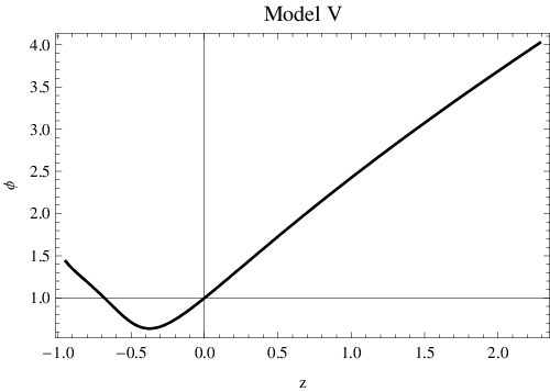
From Eqs. (81) and (82), the scale factor and the scalar field can be obtained, numerically. To do so, we take [2], , [46], [16] and use the initial values , , and . The results are plotted in Fig. 5. Figure show that (i) the scale factor is an increasing function of time , as expected for an expanding universe. (ii) The Hubble parameter and the scalar field decrease with increasing time, approach to a minimum in the future and then increase when the time increases. (iii) The deceleration parameter at late times goes to which acts like the de Sitter model. It also shows a cosmic transition from to in the future. (iv) The effective EoS parameter at late times behaves like the CDM model. It also shows the phantom divide line crossing in the future.
Using the numerical results obtained for and , the evolutionary behavior of the GSL (83) for the chameleonic BD gravity with a self interacting potential is plotted in Fig. 5(f). The figure shows that the GSL for this model is satisfied from the past to the present epoch. But in the future the GSL is violated for .
IX Conclusions
Here, we investigated the GSL in the framework of scalar-tensor gravity. In a general theory of scalar-tensor gravity, a scalar field can be nonminimally coupled both to the scalar curvature (as Brans-Dicke field) and the matter Lagrangian (as chameleon field) in the action. Hence, we extended the action of ordinary scalar-tensor gravity theory to the case in which there is a non-minimal coupling between the scalar field and the matter field. Then we derived the associated filed equations governing the gravity and the scalar field. For a FRW universe filled with the ordinary matter, we obtained the modified Friedmann equations as well as the evolution equation of the scalar field. We further assumed the boundary of FRW universe to be enclosed by the dynamical apparent horizon which is in thermal equilibrium with the Hawking temperature. Then we obtained a general expression for the GSL of gravitational thermodynamics. For some viable scalar-tensor gravity models containing BD gravity, BD gravity with a self interacting potential, chameleon gravity, chameleonic generalized BD gravity, and chameleonic BD gravity with a self interacting potential, we first obtained the evolutionary behaviors of the matter density, the scale factor, the Hubble parameter, the scalar field, the deceleration parameter as well as the effective EoS parameter. Then, we examined the validity of the GSL for the aforementioned models. Our results show the following.
(i) The aforementioned models can give rise to a late time accelerated expansion phase for the Universe. The deceleration parameter for the all models shows a cosmic deceleration to acceleration transition. In the BD gravity model, the chameleon gravity model and the chameleonic generalized BD gravity model, the cosmic transition from to occurs in the near past which is compatible with the observations [47]. For all models but the BD gravity model, at late times (), the deceleration parameter approaches a de Sitter regime (i.e. ), as expected.
(ii) The effective EoS parameter for the BD gravity model with a self interacting potential, the chameleon gravity model and the chameleonic BD gravity model with a self interacting potential, shows a transition from the quintessence state, , to the phantom regime, . For the chameleon gravity model, the transition from to occurs in the near past, as indicated by recent observations [52]. For all models but the BD gravity model, the effective EoS parameter at late times behaves like the CDM model ().
(iii) The GSL for the BD gravity model like the Einstein gravity is satisfied during the late cosmological history of the Universe. For the BD gravity model with a self interacting potential, the GSL is satisfied from the past to the present epoch. But in the future the GSL is violated for . For the BD gravity model with/without a self interacting potential, the contribution of the matter entropy in the GSL will be positive or nil for and negative otherwise. For the chameleon gravity model, the GSL is violated for the range of . However, for the horizon entropy has a positive or nil contribution in the GSL. For the chameleonic generalized BD gravity model, the GSL is violated during the late cosmological history of the Universe. Finally, for the chameleonic BD gravity model with a self interacting potential, the GSL is satisfied from the past to the present time. But in the future the GSL is violated for .
Acknowledgements
The authors thank the referee for his/her valuable comments. The works of A. Abdolmaleki and K. Karami have been supported financially by Research Institute for Astronomy and Astrophysics of Maragha (RIAAM) under research project No. 1/3569.
References
- [1]
E. Komatsu, et al., (WMAP Collaboration), Astrophys. J. Suppl. 192, 18 (2011);
G. Hinshaw, et al., (WMAP Collaboration), Astrophys. J. Suppl. 208, 19 (2013). - [2] P. Ade, et al., (Planck Collaboration) (2013), arXiv:1303.5076.
- [3] A.G. Riess, et al., Astrophys. J. 699, 539 (2009).
- [4] M. Kowalski, et al., (Supernova Cosmology Project), Astrophys. J. 686, 749 (2008).
- [5] H. Lampeitl, et al., Mon. Not. Roy. Astron. Soc. 401, 2331 (2009).
- [6]
T. Padmanabhan, Phys. Rep. 380, 235 (2003);
P.J.E. Peebles, B. Ratra, Rev. Mod. Phys. 75, 559 (2003);
C.G. Tsagas, A. Challinor, R. Maartens, Phys. Rept. 465, 61 (2008);
M. Li, X.D. Li, S. Wang, Y. Wang, Commun. Theor. Phys. 56, 525 (2011). - [7]
V. Sahni, Class. Quantum Grav. 19, 3435 (2002);
E.J. Copeland, M. Sami, S. Tsujikawa, Int. J. Mod. Phys. D 15, 1753 (2006);
T. Padmanabhan, Gen. Relativ. Gravit. 40, 529 (2008). - [8]
S. Nojiri, S.D. Odintsov, Phys. Rev. D 68, 123512 (2003);
T.P. Sotiriou, V. Faraoni, Rev. Mod. Phys. 82, 451 (2010);
S. Nojiri, S.D. Odintsov, Phys. Rept. 505, 59 (2011). - [9]
S. Nojiri, S.D. Odintsov, Phys. Lett. B 631, 1 (2005);
A.D. Felice, S. Tsujikawa, Phys. Lett. B 675, 1 (2009);
S.Y. Zhou, E.J. Copeland, P.M. Saffin, JCAP 07, 009 (2009). - [10]
S.M. Carroll, et al., Phys. Rev. D 71, 063513 (2005);
T. Koivisto, D.F. Mota, Phys. Lett. B 644, 104 (2007);
G. Cognola, et al., Phys. Rev. D 75, 086002 (2007). - [11]
G.R. Bengochea, R. Ferraro, Phys. Rev. D 79, 124019 (2009);
K. Karami, A. Abdolmaleki, Res. Astron. Astrophys. 13, 757 (2013);
K. Karami, et al., Eur. Phys. J. C 73, 2565 (2013);
K. Karami, et al., Phys. Rev. D 88, 084034 (2013). - [12] Y. Sobouti, Astron. Astrophys. 464, 921 (2007).
- [13]
Y. Fujii, K. Maeda, The Scalar-Tensor Theory of Gravitation (Cambridge University Press, Cambridge 2003);
V. Faraoni, Cosmology in Scalar-Tensor Gravity (Kluwer Academic Publishers, 2004). - [14] S. Capozziello, M. De Laurentis, Phys. Rep. 509, 167 (2011).
- [15] S. Nesseris, L. Perivolaropoulos, JCAP 01, 018 (2007).
- [16] J. Khoury, A. Weltman, Phys. Rev. D 69, 044026 (2004).
- [17]
J. Khoury, A. Weltman, Phys. Rev. Lett. 93, 171104 (2004);
P. Brax, et al., Phys. Rev. D 70, 123518 (2004). - [18]
Kh. Saaidi, H. Shaikhahmadi, Astrophys. Space Sci. 333, 501
(2011);
Kh. Saaidi, A. Mohammadi, H. Sheikhahmadi, Phys. Rev. D 83, 104019 (2011);
Kh. Saaidi, A. Mohammadi, Phys. Rev. D 85, 023526 (2012). - [19] V. Faraoni, Entropy 12, 1246 (2010).
- [20] T. Jacobson, Phys. Rev. Lett. 75, 1260 (1995).
- [21] R.G. Cai, S.P. Kim, JHEP 02, 050 (2005).
- [22]
M. Akbar, R.G. Cai, Phys. Lett. B 635,
7 (2006);
M. Akbar, R.G. Cai, Phys. Lett. B 648, 243 (2007). - [23] M. Akbar, R.G. Cai, Phys. Rev. D 75, 084003 (2007).
- [24] A. Sheykhi, JCAP 05, 019 (2009).
- [25]
R.M. Wald, Phys. Rev. D 48, 3427 (1993);
G. Cognola, et al., JCAP 02, 010 (2005);
K. Karami, M.S. Khaledian, N. Abdollahi, Europhys. Lett. 98, 30010 (2012). - [26]
R.X. Miao, M. Li, Y.G. Miao, JCAP 11, 033 (2011);
K. Karami, A. Abdolmaleki, JCAP 04, 007 (2012). - [27]
R.G. Cai, Y.S. Myung, Phys. Rev. D 56, 3466 (1997);
M. Akbar, R.G. Cai, Phys. Lett. B 635, 7 (2006). - [28] G. Izquierdo, D. Pavón, Phys. Lett. B 639, 1 (2006).
- [29]
H. Mohseni Sadjadi, Phys. Rev. D 73, 063525 (2006);
H. Mohseni Sadjadi, Phys. Rev. D 76, 104024 (2007);
H. Mohseni Sadjadi, Phys. Lett. B 645, 108 (2007);
H. Mohseni Sadjadi, Europhys. Lett. 92, 50014 (2010);
H. Mohseni Sadjadi, M. Jamil, Europhys. Lett. 92, 69001 (2010). - [30] J. Zhou, B. Wang, Y. Gong, E. Abdalla, Phys. Lett. B 652, 86 (2007).
- [31]
Y. Gong, B. Wang, A. Wang, Phys. Rev. D 75, 123516 (2007);
Y. Gong, B. Wang, A. Wang, JCAP 01, 024 (2007). - [32] M. Jamil, M. Akbar, Gen. Relativ. Gravit. 43, 1061 (2011).
- [33]
A. Sheykhi, B. Wang, Phys. Lett. B 678, 434 (2009);
A. Sheykhi, B. Wang, Mod. Phys. Lett. A 25, 1199 (2010);
A. Sheykhi, Phys. Rev. D 81, 104011 (2010);
A. Sheykhi, Eur. Phys. J. C 69, 265 (2010);
A. Sheykhi, Class. Quantum Grav. 27, 025007 (2010). - [34] N. Banerjee, D. Pavón, Phys. Lett. B 647, 447 (2007).
- [35]
K. Karami, JCAP 01, 015 (2010);
K. Karami, S. Ghaffari, Phys. Lett. B 688, 125 (2010);
K. Karami, S. Ghaffari, M.M. Soltanzadeh, Class. Quantum Grav. 27, 205021 (2010);
K. Karami, M. Jamil, N. Sahraei, Phys. Scr. 82, 045901 (2010);
K. Karami, S. Ghaffari, M.M. Soltanzadeh, Astrophys. Space Sci. 331, 309 (2011);
K. Karami, A. Sheykhi, N. Sahraei, S. Ghaffari, Europhys. Lett. 93, 29002 (2011);
K. Karami, A. Abdolmaleki, N. Sahraei, S. Ghaffari, JHEP 08, 150 (2011). - [36] N. Radicella, D. Pavón, Phys. Lett. B 691, 121 (2010).
- [37] K. Bamba, C.Q. Geng, JCAP 11, 008 (2011).
- [38] P. Peter, J.P. Uzan, Primordial Cosmology (Oxford University Press, 2009).
- [39]
E. Poisson, W. Israel, Phys. Rev. D 41, 1796 (1990);
S.A. Hayward, Phys. Rev. D 53, 1938 (1996);
Y.G. Gong, A. Wang, Phys. Rev. Lett. 99, 211301 (2007). - [40] R.G. Cai, L.M. Cao, Y.P. Hu, Class. Quantum Grav. 26, 155018 (2009).
- [41]
S. Das, P. Majumdar, R.K. Bhaduri, Class. Quantum Grav. 19, 2355 (2002);
B. Wang, C.Y. Lin, D. Pavón, E. Abdalla, Phys. Lett. B 662, 1 (2008);
D. Pavón, B. Wang, Gen. Relativ. Gravit. 41, 1 (2009);
J. Zhou, B. Wang, D. Pavón, E. Abdalla, Mod. Phys. Lett. A 24, 1689 (2009). - [42] K. Karami, S. Ghaffari, Phys. Lett. B 685, 115 (2010).
- [43] N. Radicella, D. Pavón, Gen. Relativ. Gravit. 44, 685 (2012).
- [44] C. Brans, R.H. Dicke, Phys. Rev. 124, 925 (1961).
- [45] M. Arik, M.C. Calik, M.B. Sheftel, Int. J. Mod. Phys. D 17, 225 (2008).
- [46] H. Farajollahi, et al., Astrophys. Space Sci. 337, 415 (2012).
- [47] E.E.O. Ishida, et al., Astropart. Phys. 28, 547 (2008).
- [48] R.R. Caldwell, E.V. Linder, Phys. Rev. Lett. 95, 141301 (2005).
- [49] S. Sen, A.A. Sen, Phys. Rev. D 63, 124006 (2001).
- [50] H. Farajollahi, A. Salehi, Int. J. Mod. Phys. D 19, 621 (2010).
- [51] H. Farajollahi, A. Salehi, F. Tayebi, Can. J. Phys. 89, 915 (2011).
- [52]
U. Alam, V. Sahni, A.A. Starobinsky, JCAP 06, 008 (2004);
D. Huterer, A. Cooray, Phys. Rev. D 71, 023506 (2005);
Y. Wang, M. Tegmark, Phys. Rev. D 71, 103513 (2005). - [53] N. Banerjee, D. Pavón, Phys. Rev. D 63, 043504 (2001).
- [54] A. Sheykhi, M. Jamil, Phys. Lett. B 694, 284 (2011).