phase diagram of three-dimensional disordered topological insulator via scattering matrix approach
Abstract
The role of disorder in the field of three-dimensional time reversal invariant topological insulators has become an active field of research recently. However, the computation of invariants for large, disordered systems still poses a considerable challenge. In this paper we apply and extend a recently proposed method based on the scattering matrix approach, which allows the study of large systems at reasonable computational effort with few-channel leads. By computing the invariant directly for the disordered topological Anderson insulator, we unambiguously identify the topological nature of this phase without resorting to its connection with the clean case. We are able to efficiently compute the phase diagram in the mass-disorder plane. The topological phase boundaries are found to be well described by the self consistent Born approximation, both for vanishing and finite chemical potential.
pacs
72.10.Bg, 72.20.Dp, 73.22.-fI Introduction
Time reversal invariant (TRI) topological insulators, a class of insulating materials with strong spin orbit coupling, have attracted a great amount of attention in recent years. While clean systems are fairly well understood,[1, 2] an important theme in current topological insulator research is the study of disorder. Besides being crucial for the interpretation of experimental data, disorder is of fundamental interest: Generically, disorder localizes electron wavefunctions and thus is expected to counteract non-trivial topology, which, as a global property, requires the existence of extended wavefunctions in the valence and conduction bands. One of the defining properties of strong topological insulator (STI) phases is their unusual stability: extended bulk- and gapless edge electronic states persist for weak to moderately strong disorder. With increasing disorder strength, the bulk gap gets filled with localized electronic states, the mobility gap decreases and finally, at the topological phase transition, the mobility gap closes and the surface states at opposite surfaces gap out via an extended bulk wavefunction.[3]
However, disorder physics in topological insulators is much richer than suggested by the simple scheme above. A drastic example is provided by the topological Anderson insulator transition, where increasing disorder drives an ordinary insulator (OI) into a topologically nontrivial phase.[4, 5, 6, 14, 7] Moreover, the role of different disorder types [8] or spatially correlated disorder [9] has been addressed in literature. Further, weak topological insulator (WTI) phases known to be protected by translational symmetry were shown to be surprisingly stable against almost all disorder types allowed by discrete symmetries. [10, 11, 12]
One of the challenges in the field of disordered topological insulators is the computation of the invariants that characterize strong and weak topological insulator phases. (Without disorder, the invariants can be computed directly from the band structure.[13, 1, 2]) While methods based on exact diagonalization are applicable for two dimensional systems, their performance for three-dimensional systems is rather poor[14, 15, 16]. For example, a recent study [16] was only able to map the invariant for a few lines in the disorder strength–Fermi energy plane for a system of 8x8x8 lattice sites, leaving uncertainties about the possibility to infer qualitative and quantitative behavior in the experimentally relevant thermodynamic limit. As an example of an indirect method for calculating the invariant, the three-dimensional topological Anderson insulator was argued to be topological nontrivial by employing the Witten effect.[7] The transfer-matrix method can be used to obtain Lyapunov exponents in a finite-size scaling analysis,[17, 18] which is then used to infer information on topological phase boundaries. Drawbacks of this method include difficulties in the determination of the phase boundary between two insulating phases, since size dependence of the decay length is intrinsically small on both sides of the transition. In the case of a transition between an insulating topologically trivial and nontrivial phase, application of open boundary conditions allows for a facilitated detection of the resulting insulator-(surface)metal transition. However, this causes a much stronger finite-size effect and renders the interpretation of the results for finite system sizes rather difficult. For example, a recent transfer-matrix study [19] speculates about a novel “defeated WTI” region in the phase diagram, whose precise nature and properties have not been finally resolved.
As a numerically inexpensive alternative, Fulga et al. proposed to obtain the topological invariants from a topological classification of the scattering matrix of a topological insulator.[20] As a Fermi surface quantity, the computational requirements for the calculation of the scattering matrix scale favorably, so that it is accessible with modest effort. The method requires the application of periodic boundary conditions and considers the dependence of the scattering matrix on the corresponding Aharonov-Bohm fluxes. In two dimensions, there is only one flux, and the method effectively classifies a “topological quantum pump”,[21, 22, 23] via a mapping similar to that devised by Laughlin to classify the integer quantized Hall effect.[24]
In this article, we report on the application of a scattering matrix-based approach to a disordered three-dimensional topological insulator model [25, 26, 27] that features both strong and weak topological insulator phases. In Sec. II we review the theory and discuss the practical implementation of the method, which more closely follows the ideas of Ref. 22, and differs from that of Ref. 20 at some minor points. The relation to the band-structure-based approach is discussed in Sec. III. In section IV we present the phase diagram in the mass–disorder strength plane. In contrast to Ref. 19 we see no evidence of a “defeated WTI” phase. We conclude in section V. Two appendices contain details on analytic modeling of the scattering matrix for the clean limit and an assessment of finite-size effects.
II Scattering theory of three-dimensional topological insulators
The tight-binding model we consider is a variant of the widely-used low-energy effective Hamiltonian of the material family.[25, 26, 27] In the absence of disorder the momentum-representation Hamiltonian reads
| (1) | |||||
where Pauli matrices and refer to spin- and orbital degrees of freedom, respectively. For definiteness, we set and choose energy units such that . The system has time reversal symmetry, , inversion symmetry, , and, if , particle-hole symmetry . Here is the time-reversal operator ( complex conjugation, ), the inversion operator, and the particle-hole conjugation operator ().
The full Hamiltonian
| (2) |
includes an on-site disorder potential that respects time reversal symmetry. The most general form of the disorder potential is
| (3) |
where the summation is over all lattice sites , and . The amplitudes are drawn from a uniform distribution in the interval . The disorder potential breaks inversion symmetry; the terms , , , and also break particle-hole symmetry. We consider a lattice of size and apply periodic boundary conditions in the and directions, but open boundary conditions at the surfaces at and . Below, we first discuss the case of potential disorder only (, for ), and return to the other disorder types at the end of our discussion.
Our main focus will be on the case where, without disorder, three different topological phases appear inside the parameter range , which is the parameter range we consider here. For the model is in the WTI phase, with topological indices ; for it is in the STI phase with indices ; for the system is in the OI phase with indices . The inversion symmetry of the clean model with ensures that bulk gap closings exist at the topological phase transitions at and only.[28]
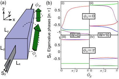
In order to obtain a scattering matrix, we open up the system by attaching two semi-infinite, translation- and time-reversal invariant leads to both surfaces orthogonal to, say, the -direction, as shown in Fig. 1(a). The leads are described by a tight-binding model, defined on the same lattice grid as the bulk insulator. In principle, for the scattering matrix method, the leads can be generic and are to be chosen as simple as possible for fast computation. However, for reasons related to numerical robustness, we choose a lead that is one site wide in the direction, but two sites wide in the direction. (We refer to Appendix A for a detailed discussion why in this case a strictly one-dimensional chain is less well suited for the purpose of topological classification.) The coordinates of the lead sites are and . Without loss of generality, the and coordinates of the lead sites are fixed at and , . Using and to denote unit vectors in the and directions, respectively, the Hamiltonian for the left lead reads (see also Appendix A)
| (4) | |||||
with lattice vector . In our calculations we have set and . For this choice of parameters the lead supports four right-propagating modes and their left-propagating time reversed partners. The coupling between the leads and the bulk sample is described by the coupling term
| (5) |
with . Similar expressions apply to the Hamiltonian of the right lead and the coupling between the right lead and the sample. In our calculations we have chosen the value , optimized empirically for the numerical detection of the scattering resonances.
To find the topological invariants for a disordered sample, we employ the twisted boundary conditions method.[29, 16] This amounts to inserting additional phase factors and in the hopping matrix elements connecting sites at and , and and , respectively. The resulting system can be thought of as a large unit cell defined on a torus with two independent Aharonov-Bohm fluxes threading the two holes around the and axes. For the purpose of classifying insulating phases it is sufficient to focus on the reflection matrix of the left () lead, which is a unitary matrix for an insulating sample. For our choice of parameters, the leads have four propagating modes at the Fermi energy (), so that is a matrix.
To obtain topological invariants from the scattering matrix, we note that, because of time-reversal invariance, satisfies the condition
| (6) |
where denotes the matrix transpose and the unitary matrix describes the action of the time reversal operator in the space of scattering states.[20] Since flips the sign of the velocity , it connects incoming and outgoing modes, . Reference 20 chooses a convention wherein, after redefinition of the incoming scattering states, the scattering matrix becomes antisymmetric at the “time-reversal invariant fluxes” , and, thus, acquires the same symmetry properties as the matrix used by Fu and Kane to classify time-reversal invariant topological insulators without disorder in terms of their band structure.[13] Here, we follow the formulation of scattering theory as it is most commonly used in the theory of quantum transport,[30, 31] in which one makes the choice . At the time-reversal invariant fluxes this gives the condition that is “self dual”, . Then Kramers degeneracy ensures that the eigenphases of are twofold degenerate at . The topological classification rests on the eigenvalue evolution as one of the fluxes or changes from to , so that the system evolves from one time-reversal invariant flux configuration into another one:[23] In the topologically trivial case, labeled by , degenerate eigenvalue pairs, which generically split upon departing from a time-reversal invariant flux, are reunited upon reaching the other time-reversal invariant fluxes. In the nontrivial case, which we label by , the eigenphases from a degenerate pair are united with eigenphases from different pairs. (If is a matrix, so that there is only a single eigenvalue pair, the question of topological triviality is connected to the winding of the eigenphase pair around the unit circle.[23]) One easily verifies that this definition is independent of the choice which eigenphase pair is being “tracked”: if one eigenphase pair “switches partners”, then all eigenphase pairs must do so. Similar considerations have been applied to Kramers degenerate energy level pairs in order to argue for topological non-triviality of time-reversal invariant topological insulators.[21, 13, 32] The strong and weak topological invariants of the sample are then defined as[20]
| (7) | |||||
| (8) | |||||
| (9) |
The two expressions for are equivalent, because the evolution of an eigenphase pair for a contractable loop in the , -plane is always trivial. The relations (7)–(9) remain valid under circular permutation of spatial indices, so that, e.g., the weak topological index can be calculated by attaching a lead in the or directions.
Using the Kwant software package,[33] we performed numerical calculations of and on a system with dimensions and variable . Here the length was increased until an (almost) unitary reflection matrix was found, where we used the condition as an empirical cut-off where unitarity is reached. The possibility of large system sizes is needed to accommodate cases with a long localization length, as it occurs close to a topological phase transition. If the condition could not be met for the system is empirically labeled as metallic. (Note that a full assessment of the metal/insulator transition requires an analysis of the scaling behavior of conductivity, which is beyond the scope of this work.) The approach to a unitary scattering matrix is illustrated in Fig. 2, which shows the evolution of as a function of at disorder strength across the OI-STI transition for three different values of . During the sweep of the flux and , the eigenphases have been tracked using a dynamical step-width control, allowing to resolve sharp features in the eigenphase trajectory. Note that the use of twisted boundary conditions in the and directions allows us to chose moderate , since we are not required to separate any surface states. We found the system size , sufficient to suppress finite-size issues: Beyond a parity effect for (see the discussion in the next section) there is no dependence of the results on increased , see Appendix B.
As an example, Fig. 1(b) shows a typical eigenphase evolution for and in the clean and a disordered case ( and ). For a topologically nontrivial winding is obtained, while shows a trivial winding for both the clean and the disordered case. With Eqs. (7) and (9) we obtain and , respectively. Similarly, we confirmed which, in summary, leads to for the particular points in parameter space.
III Comparison with band-structure-based approach
In this section, we focus on . For a clean bulk system, the topological indices and can also be calculated from the band structure. The weak indices one obtains from the scattering approach agree with those for the bulk system if and only if the sample dimensions , , and are odd. (For even sample dimension, the scattering method yields trivial weak indices.) The advantage of the scattering approach is that the weak indices can be calculated for a disordered system as well.
In order to show that the scattering-matrix-based topological indices of Eqs. (7)–(9) are the same as the band-structure based indices if the sample dimensions are odd, we make use of the relation between scattering phases and bound (surface) states: A surface state exists at energy if and only if for energy has an eigenphase . This relation follows from the observation that capping the lead by a “hard wall”, which has scattering matrix , restores the original surface state spectrum without coupling to an external lead. A nontrivial winding requires that an odd number of eigenphases passes the reference phase upon sweeping the fluxes and as specified in Eq. (7)–(9), whereas an even number of eigenphases passes the reference phase if the winding is trivial.[23] Note, that depending on the definition of the lead modes, the numerical value of the reference phase might differ from . (In Appendix A, we show that for the clean and weak coupling limit all phase winding signatures can be reproduced quantitatively from an analytical calculation of the scattering matrix in terms of the surface states at the surface.)
In a clean system, translation invariance in the and directions implies that the surface states are labeled by a wave-vector in the surface Brillouin zone. Possible Dirac cones in the plane are centered around the four time-reversal-invariant momenta , , , and , see Fig. 3. For a finite-size sample with twisted boundary conditions, only discrete values , are allowed. A resonance (i.e. scattering phase ) is found if one of the allowed vectors crosses one of the surface Dirac cones.
For definiteness, we now consider the weak index , which is determined by the phase winding along the path at fixed . While sweeping , the allowed values build a set of trajectories in the plane, which are shown in Fig. 3 for the cases of and even or odd. From inspection of Fig. 3 one immediately concludes, that a Dirac cone gives rise to an odd number of scattering resonances if and only if its center is at one of the “allowed” vectors for or for , which requires odd for Dirac points with . Hence, we conclude that if and only if is odd, the index of Eq. (9) measures the parity of the number of Dirac points with . Similarly, the index of (8) measures the parity of the number of Dirac points with if and only if is odd, whereas the index of Eq. (7) measures the parity of the total number of Dirac points for both even and odd sample dimensions. In all three cases, the parities of number of Dirac points corresponds to the very same quantities as those that are computed from the band structure.[34, 1, 2]
There is a simple argument that shows that the scattering-matrix-based weak indices are always trivial if the sample dimensions are even, irrespective of the value of the bulk index: Any three-dimensional weak topological insulator is adiabatically connected to a stack of two dimensional topological insulators. The stacking direction can be taken to be . A “mass term” that couples these layers in pairs connects the system adiabatically to a trivial insulator.[10, 11, 35] If , , are all even, such a mass term can be applied for any . Since the indices of Eqs. (8) and (9) are true topological invariants, they cannot change upon inclusion of such a mass term, i.e., they can only acquire a value compatible with the topologically trivial phase.
For odd sample dimensions this argument does not apply and, as is shown above, for the clean case, the topological indices derived from the scattering matrix agree with the indices obtained from the band structure.
IV Phase diagram in the presence of disorder
We now discuss the phase diagram of the three-dimensional Hamiltonian in the parameter plane with potential disorder. We study the cases and . Topological indices and are computed as described in Sec. II for a dense grid of parameter values. The result is shown in Fig. 4. For , it confirms similar topological phase diagrams computed on the basis of conductance and scaling methods as in Refs. 17, 19. Due to the large maximum system size of we relied on self averaging and worked with only a single disorder realization per point in parameter space. The results indicate that this is indeed justified for the range of weak and moderate disorder strengths; only for the strong disorder region , where Anderson localization and a trivial insulator is expected, a minority of data points yields diverging results.
Studies of disorder effects of the three-dimensional quantum critical point between STI and OI at employing the self consistent Born approximation[3], renormalization group[36] or a numerical approach[37] show the existence of a critical disorder strength below which a direct phase transition without extended metallic phase is realized. This conclusion however is valid only for systems with chemical potential at the clean band-touching energy (here ) which also preserve inversion symmetry (after disorder average). Indeed, our numerical results for show that the width of the metal region at the -induced transition between WTI, STI and OI, for weak disorder is considerably smaller than in other studies of the invariant for disordered systems,[16, 20] indicating that finite-size effects are much less severe for the large system sizes we can reach. Further indication for the successful suppression of finite-size effects is that the phase diagram in Fig. 4(a) remains unchanged if we increase the system volume by to , see Appendix B.)
An analytical approach to disordered topological insulators is the calculation of the disorder averaged self-energy using the self-consistent Born approximation (SCBA).[3, 7] Due to symmetry arguments, can be expanded as , where is the unit matrix, and the SCBA equation reads [7, 3]
| (10) |
where the notation was introduced below Eq. (3). Consequently, the disorder averaged propagator features renormalized mass and chemical potential values and , respectively. If and in the bands above and below energies the system is metallic; otherwise, if is in the bandgap, the value of determines the nature of the resulting insulator: For we expect an OI, yields a WTI and indicates a STI. Nonzero imaginary parts, and translate into a finite lifetime and a finite density of states at the Fermi level, indicating either a compressible diffusive metal phase[36] or, if these states are localized, an insulator. SCBA cannot distinguish between both possibilities.
The coupled set of SCBA equations (10) is numerically solved self-consistently. For potential disorder ( for ), the resulting phase boundaries of insulating phases with are shown in Fig. 4 as solid lines. For , we find excellent agreement of the SCBA phase boundaries with the results from the scattering matrix method. Since SCBA as a disorder-averaged theory is free of finite size effects, this further supports the applicability of the scattering matrix results in the thermodynamic limit. The situation is different for , where for strong disorder () the insulating states slightly but numerically significantly exceed the regions where as obtained from SCBA, indicating localized states at the Fermi energy. A similar observation was reported in Ref. 16.
In closing, we comment on the effect of the five remaining disorder types. By inspection of Eq. (10) we find that mass-type disorder, , has the same effect as pure potential disorder, i.e., bending the phase boundaries between insulating phases to increased values of . All other disorder types have the opposite effect on , as was noticed for the two dimensional case in Ref. 8. We have confirmed the agreement between scattering matrix results and the trends predicted by SCBA in these cases (results not shown). We conclude that qualitative features of the phase diagram, like, for example, the occurrence of a disorder-induced topological Anderson insulator transition, crucially rely on the microscopic details of the disorder potential.
V Conclusion
We have demonstrated the potential of the scattering matrix method for the computation of topological indices for a three-dimensional disordered tight-binding model featuring strong and weak topological phases. We studied the phase diagram in the mass - disorder plane for system sizes up to and found excellent agreement with SCBA predictions. The latter have been studied in the literature before[3, 36, 17] (only for the OI/STI case and for ) but have never been compared quantitatively to a real-space disordered three-dimensional TI tight-binding model. We conclude that SCBA should have predictive value also for similar scenarios. In particular, we showed that SCBA is quantitatively correct also for finite chemical potential and weak disorder, where extended metal regions occur even for weak disorder, whenever the (renormalized) chemical potential lies within a bulk band. This possibility has been overlooked in Ref. 18. For the insulator-metal transition at larger disorder strength, SCBA’s precision suffers from its inherent inability to take into account localization effects[18] which occur at the edges of topological nontrivial bands.
The scattering matrix method can be regarded as complementary to a finite-size scaling analysis. While the latter is ideally suited to detect a phase boundary, the scattering matrix method can unambiguously identify the topological phase at each parameter point where the system is insulating. This proves the nontrivial nature of the TAI phase without referring to adiabatic connection to the clean STI phase or involving other indirect arguments. For the disordered WTI, we find no evidence for a “defeated WTI” region in the phase diagram, as suggested recently in Ref. 19. We point out that the scattering matrix method should be an ideal tool to identify the topological invariants for (so far hypothetical) disordered topological phases that are not adiabatically connected to the clean case.
The scattering matrix method is able to find weak indices even if the strong index is nonzero, as has been checked using a modified Hamiltonian (as in Ref. 27) with anisotropic mass parameters which realizes many more topological phases, e.g. . Moreover, our results explicitly demonstrate the intricate interplay between system size and topological phase in the parameter region supporting a WTI phase. Adding a single layer to the system can change the topological phase from OI to WTI or vice versa, a behavior not reflected in conductance simulations. The case of a disordered WTI phase has been previously discussed in Refs. 38, 39, where it is argued that average translational symmetry in stacking direction is sufficient to protect the weak topological insulator phase. This is in agreement with our findings since an odd number of stacked layers prohibits any average translational symmetry breaking while such a dimerization can be adiabatically applied to an even number of layers.
Acknowledgements.
We thank A. Akhmerov, C. Groth, X. Waintal and M. Wimmer for making the Kwant software package available before publication. We thank a thoughtful referee for pointing out the problem with SCBA in Ref. 18. Financial support was granted by the Helmholtz Virtual Institute “New states of matter and their excitations” and by the Alexander von Humboldt Foundation in the framework of the Alexander von Humboldt Professorship, endowed by the Federal Ministry of Education and Research.Appendix A Analytic modeling of the phase winding in the clean limit
In the clean case, it is possible to understand the scattering matrix eigenvalue phase winding signatures (and thus the topological classification) from a microscopic point of view. We employ the Fisher-Lee relation[40] to calculate the elements of the scattering matrix from the retarded Green function ,
| (11) |
where the right hand side represents the current in outgoing lead mode after a normalized local excitation of incoming mode . The mode velocities and link this quantity to the usual amplitude propagation described by and any direct transition into outgoing modes (, not contributing to the system’s scattering matrix) is subtracted. The Green function depends on the scattering region (i.e. the topological insulator surface), the lead and their mutual coupling. We first discuss the effective description of the topological insulator surface and specify a simplified lead . We then compare the analytical prediction with the full-scale numerical calculation. Finally we motivate the lead choice in the main text, .
A.1 Surface states and surface Hamiltonian
Following the convention of the main text, we consider a clean topological insulator described by Eq. (1), occupying the half space . We make the same parameter choice as described in Sec. II. For energies in the bulk gap, a description in terms of the effective surface theory is sufficient. The Bloch wavefunctions for the surface states at surface momentum close to a Dirac point at momentum can be found using the method applied in Ref. 35. For the STI () the two surface states around the single Dirac point at read
in the same basis as Eq. (1) and with a normalized, decaying function for .[35] In the basis of these two Bloch states, the effective surface Hamiltonian becomes a matrix which reads
| (22) |
The constant was defined in Eq. (1).
For the WTI () there are four surface bands, which form two Dirac cones centered around and . The basis states are the same as in Eqs. (A.1) and (A.1), but with surface momenta defined around for , respectively. We find
| (23) |
In a system with finite and given fluxes , a finite subset of surface wave-vectors are compatible with the twisted boundary conditions, see the discussion in Sec. III. During the sweep of the “flux” or , the allowed values form a set of trajectories in the surface Brillouin zone, see Fig. 3. For an approximate description of the scattering process, it is sufficient to further restrict the effective surface Hamiltonian to the few allowed wave-vectors on trajectories which are closest to the Dirac points. As we will show momentarily, the arrangement of the trajectories in the surface Brillouin zone relative to the locations of the gapless points then determines the phase winding structure.
A.2 Lead and its self-energy
The leads are modeled as semi-infinite, translational- and time-reversal invariant tight-binding systems. To motivate the special choice of lead described by Eq. (4), we first consider a simpler (thinner) lead as in Fig. 5(a), realized as a tight binding chain of lattice sites at coordinates , with and Hamiltonian
| (24) |
where . The wavefunctions of the four scattering channels at the four Fermi points and are denoted , with . They are chosen such that the matrix , defined below Eq. (6), fulfills the condition . Finally, the lead is coupled to the system (i.e. the topological insulator) by times a real constant ,
| (25) |
for .
For a semi-infinite lead, the retarded Green function is an infinite dimensional matrix. However, employing the concept of lead self-energy,[41] the degrees of freedom corresponding to the lead can be eliminated. The calculation of the Green function in Eq. (11) is most efficient if we retain the lead site . Thus, the lead self-energy should take into account only lead sites . It reads[41] where is the Green function of the lead without the coupling . Finally, at zero energy we have and
| (26) |
where and are incoming and outgoing scattering states for the lead terminated at , i.e. without the coupling .
A.3 STI phase
As a first specific example we consider the case of a strong topological insulator, for which the surface Hamiltonian has a single Dirac cone centered at . We chose since then , see Ref. 35. Employing the boundary conditions for, say, and odd, the resulting trajectories for the surface momenta are shown in Fig. 6 (inset). For the effective low energy theory (encircled region in the surface Brillouin zone) we find from Eq. (22)
| (27) |
In order to calculate the Green function we assume weak system-lead coupling . Then can be approximated by the ideal effective surface theory without lead, Eq. (27), and we find in the basis of Eq. (27) and Eq. (24)
Finally, Eq. (11) yields
| (28) |
where . The resulting Eigenvalue phase winding is compared to the full-scale numerical calculation in Fig. 6, the excellent agreement between both curves quantitatively confirms the model leading to Eq. (28). For larger coupling strength [i.e. as used in the numerics for Figs. 1(b) and 4], the assumption becomes invalid as surface states strongly hybridize with the lead and can no longer be labeled with surface momenta. Accordingly, Eq. (28) then deviates from the full numerical solution.
The phase winding shown in Fig. 6 (STI, and ) is nontrivial. In a similar fashion, all other phase windings in the absence of disorder can be modeled using the effective low-energy and agree with the kwant results. In general, a surface momentum trajectory that leaves or enters an odd number of surface Dirac points corresponds to a non-trivial phase winding. In the following, as we discuss the only case where two Dirac points are reached for the same flux configuration, we show why we prefer using the extended lead [Eq. (4)] instead of the strictly one-dimensional lead [Eq. (24)].
A.4 Motivation for an extended lead
Consider the situation and even system dimensions. For and the trajectories of surface momenta simultaneously leave the two Dirac cones at and , respectively. The effective surface Hamiltonian is
| (29) |
with basis states in Eqs. (A.1) and (A.1) for , . Now consider a lead which is weakly coupled to just a single site at the surface of the system, say at , and calculate the Green function . Crucially, the coupling matrix elements (denoted by in the following) for the two different surface Dirac cones are identical in such a situation since they fail to resolve the different in-plane momenta of the surface states. Representing the 2x2 blocks of Eq. (29) by we obtain generically
| (30) |
where (after matrix inversion) the relevant on-site part at is just , leading to a scattering matrix independent of . This trivial phase winding is consistent with the discussion in Sec. III. However, any small perturbation that acts differently on the two Dirac cones invalidates the exact cancellations and causes a steep but still trivial phase winding that is increasingly harder to track for a decreasing perturbation strength. In numerical practice, finite precision of the arithmetics plays the role of a tiny perturbation which prevents proper eigenvalue phase tracking. Although even a small amount of disorder () is a sufficiently strong perturbation to overcome the problem, an improved lead and lead-system coupling than can distinguish between the two surface Dirac cone basis states are desirable.
A lead which is extended in, say, direction [see Fig. 5(b)] can carry modes that probe the different in-plane momenta of surface states. Such a lead is realized by our default choice in Eq. (4). The modes are proportional to or and are thus mutually orthogonal to the the surface modes if these belong to Dirac cones with or . Thus, the scattering scenario described in this section becomes an effective double copy of the scenario in Subsection A.3. Now, the steepness of the (double) phase winding is conveniently controlled by , which justifies the increased numerical cost due to the doubling of scattering channels.
Appendix B Finite-size effects
References
- [1] M. Z. Hasan, C. L. Kane, Rev. Mod. Phys. 82, 3045 (2010).
- [2] B. A. Bernevig, Topological Insulators and Topological Superconductors (Princeton University Press, 2013).
- [3] R. Shindou, S. Murakami, Phys. Rev. B 79, 045321 (2009).
- [4] J. Li, R.-L. Chu, J.K. Jain, S.-Q. Shen, Phys. Rev. Lett. 102, 136806 (2009).
- [5] H. Jiang, L. Wang, Q-f. Sun, X.C. Xie, Phys. Rev. B 80, 165316 (2009).
- [6] C. Groth, M. Wimmer, A. Akhmerov, J. Tworzydlo, C. Beenakker, Phys. Rev. Lett. 103, 196805 (2009).
- [7] H.-M. Guo, G. Rosenberg, G. Refael, M. Franz, Phys. Rev. Lett. 105, 216601 (2010).
- [8] J. Song, H. Liu, H. Jiang, Q.-F. Sun, X. C. Xie, Phys. Rev. B 85, 195125 (2012).
- [9] A. Girschik, F. Libisch, S. Rotter, Phys. Rev. B 88, 014201 (2013).
- [10] Z. Ringel, Y. E. Kraus, A. Stern, Phys. Rev. B 86, 045102 (2012).
- [11] R. S. K. Mong, J. H. Bardarson, J. E. Moore, Phys. Rev. Lett. 108, 076804 (2012).
- [12] H. Obuse, S. Ryu, A. Furusaki, C. Mudry, arxiv:1310.1534 (2013).
- [13] L. Fu, C. Kane, Phys. Rev. B 76, 045302 (2007).
- [14] H.-M. Guo, Phys. Rev. B 82, 115122 (2010).
- [15] M. B. Hastings, T. A. Loring, Ann. Phys (NY) 326, 1699 (2010).
- [16] B. Leung, E. Prodan, Phys. Rev. B 85, 205136 (2012).
- [17] S. Ryu, K. Nomura, Phys. Rev. B 85, 155138 (2012).
- [18] A. Yamakage, K. Nomura, K.-I. Imura, Y. Kuramoto, Phys. Rev. B 87, 205141 (2013).
- [19] K. Kobayashi, T. Ohtsuki, K.-I. Imura, Phys. Rev. Lett. 110, 236803 (2013).
- [20] I. C. Fulga, F. Hassler, A. R. Akhmerov, Phys. Rev. B 85, 165409 (2012).
- [21] L. Fu, C. Kane, Phys. Rev. B 74, 195312 (2006).
- [22] D. Meidan, T. Micklitz, P. W. Brouwer, Phys. Rev. B 82, 161303 (2010).
- [23] D. Meidan, T. Micklitz, P. W. Brouwer, Phys. Rev. B 84, 195410 (2011).
- [24] R. Laughlin, Phys. Rev. B 23, 5632 (1981).
- [25] H. Zhang, et al., Nat. Phys. 5, 438 (2009).
- [26] C.-X. Liu, et. al., Phys. Rev. B 82, 045122 (2010).
- [27] K.-I. Imura, M. Okamoto, Y. Yoshimura, Y. Takane, T. Ohtsuki, Phys. Rev. B 86, 245436 (2012).
- [28] S. Murakami, New J. Phys. 9, 356 (2007).
- [29] Q. Niu, D. Thouless, Y.-S. Wu, Phys. Rev. B 31, 3372 (1985).
- [30] C. Beenakker, Rev. Mod. Phys. 69, 731 (1997).
- [31] Y. Nazarov, Y. V. Blanter, Theory of Quantum Transport (Cambridge University Press, 2009).
- [32] K. Nomura, M. Koshino, S. Ryu, Phys. Rev. Lett. 99, 146806 (2007).
- [33] C. W. Groth, M. Wimmer, A. R. Akhmerov, X. Waintal, arxiv:1309.2926v1 (2013).
- [34] L. Fu, C.L. Kane, E. Mele, Phys. Rev. Lett. 98, 106803 (2007).
- [35] C.-X. Liu, X.-L. Qi, S.-C. Zhang, Physica E 44, 906 (2012).
- [36] P. Goswami, S. Chakravarty, Phys. Rev. Lett. 107, 196803 (2011).
- [37] K. Kobayashi, T. Ohtsuki, K.-I. Imura, I. F. Herbut, Phys. Rev. Lett. 112, 016402 (2014).
- [38] L. Fu, C. L. Kane, Phys. Rev. Lett. 109, 246605 (2012).
- [39] I. C. Fulga, B. van Heck, J. M. Edge, A. R. Akhmerov arxiv:1212.6191v3 (2012).
- [40] D. Fisher, P. Lee, Phys. Rev. B 23, 6851 (1981).
- [41] S. Datta, Electronic Transport in Mesoscopic Systems (Cambridge University Press, 1997).