跳到论文正文
W Papers独立论文阅读器 arXiv:1401.7204 论文正文 计算阅读时间 · 0%
引用这篇论文根据当前论文元数据生成,正式投稿前建议核对。


License: arXiv.org perpetual non-exclusive license
arXiv:1401.7204v2 [hep-ph] 23 Jul 2014

One loop radiative correction to Kaluza-Klein masses
in S2/Z2S^{2}/Z_{2} universal extra dimensional model

Preprint: OCU-PHYS 397, STUPP-14-216
Nobuhito Maru Email: nmaru@sci.osaka-cu.ac.jp Affiliation: Department of Mathematics and Physics, Osaka City University, Osaka, 558-8585, Japan    Takaaki Nomura Email: nomura@mail.ncku.edu.tw Affiliation: Department of Physics, National Cheng-Kung University, Tainan 701, Taiwan    Joe Sato Email: joe@phy.saitama-u.ac.jp Affiliation: Department of Physics, Saitama University, Shimo-Okubo, Sakura-ku, Saitama 355-8570, Japan
August 24, 2026
Abstract

We investigate a radiative correction to the masses of Kaluza-Klein(KK) modes in a universal extra dimensional model which are defined on a six-dimensional spacetime with extra space as a two-sphere orbifold S2/Z2S^{2}/Z_{2}. We first define the Feynman rules which are necessary for the calculation. We then calculate the one-loop diagrams which contribute to the radiative corrections to the KK masses, and obtain one-loop corrections to masses for fermions, gauge bosons and scalar bosons. We estimate the one-loop corrections to KK masses for the first KK modes of standard model particles as a function of momentum cut-off scale, and we determine the lightest KK particle which would be a promising candidate of a dark matter.

Keywords: 
extra dimension, universal extra dimension model, dark matter

I Introduction

The Standard Model(SM) has been well established. It has indeed passed test of the accelerator experiments. It is, however, not a satisfactory theory for all the physicists. There seems to be several flaws, e.g., the hierarchy problems, no candidate of dark matter, and so on. With the fact that relic abundance of the dark matter is well explained by weakly interacting massive particle, these problems strongly indicate a new physics beyond the SM at TeV scale.

There are many candidates of such models, say, models with supersymmetry, little higgs, extra dimensions, and so on. Since the Large Hadron Collider experiment is now operating, which will explore the physics at TeV scale, it is urgent to investigate possible models at that scale.

Among these, the idea of Universal Extra Dimensional(UED) model is very interesting [1, 2]. The minimal version of UED has recently been studied very extensively. It is a model with one extra dimension defined on an orbifold S1/Z2S^{1}/Z_{2}. This orbifold is given by identifying the extra spatial coordinate yy with −y-y and hence there are fixed points y=0,πy=0,\pi. By this identification chiral fermions are obtained. It is shown that this model is free from the current experimental constraints if the scale of extra dimension 1/R1/R, which is the inverse of the compactification radius RR, is larger than 400 GeV [1, 3]. The dark matter can be explained by the first or second Kaluza-Klein (KK) mode [4], which is often the first KK photon, and this model can be discriminated from other models [5]. This model can also give plausible explanations for SM neutrino masses which are embedded in extended models [6].

In contrast with the UED models in five dimensions, UED models in six dimensions have interesting properties which would explain some problems in the SM. For example, in six dimensions, the number of generations of quarks and leptons is derived by anomaly cancellations [7] and the proton stability is guaranteed by a discrete symmetry of a subgroup of six dimensional Lorentz symmetry [8]. Candidate of UED models in six dimensional model are the one with extra dimensions of T2T^{2}, a torus[1], or the one with S2S^{2}, a sphere[9, 10]. In these two classes of models, the latter is quite new and its phenomenology has been studied recently in Refs. [11, 12, 13, 14].

Although we do not have experimental hints of existence of extra dimensions presently, it is meaningful to explore non-minimal UED models. There are many kind of UED models and we should know the properties for different models to test them in experiments. For example, we can explore preferred KK mass scale by estimating relic density of dark matter for each UED models using KK mass spectrum and couplings, and it will suggest what values of KK masses we can expect to discover at collider experiments. Thus it is important to investigate properties of each UED models such as mass spectrum and couplings to examine the validity of the UED in experiments. Furthermore, S2S^{2} has the structure of the simplest coset space SU(2)/U(1) and it has been applied in Coset Space Unification scenario [15, 16] to construct unified models. Thus it is worth investigating the radiative corrections to mass spectrum of the KK modes even apart from UED models.

To study it in detail, first of all we have to calculate the quantum correction to mass spectrum. It is well known that at tree level all the particles in the same Kaluza-Klein (KK) mode are degenerate in mass and therefore it is impossible to predict even a decay mode. It is hence inevitable to calculate the quantum correction to their mass to find its phenominological consequences, say, collider signatures. This small correction relative to their tree mass is crucial since mass differences by it is “infinitely” large campared with it at tree level, and hence it determines physics. In five-dimensional model, radiative corrections to KK masses and couplings are discussed in [17] where the importance of choice of regulator is taken into account [18]. For UED model, the aurthors of [19] have calculated the radiative corrections in S1S^{1} and T2T^{2}. Also the running Higgs self couplings and Yukawa couplings are discussed in [20] for T2T^{2} UED and in [14] for S2S^{2}-based UED models. However there is no calculation of the corrected KK masses for the S2S^{2} model[9].

In models with two sphere, fermions cannot be massless because of the positive curvature and hence they have a mass of O(1/R1/R) [21, 22]. We cannot overcome the theorem simply by the orbifolding of the extra spaces. In usual cases, we have no massless fermion on the curved space with positive curvature, but we know a mechanism to obtain a massless fermion on that space by introducing a nontrivial background gauge field [23, 24]. The nontrivial background gauge field can cancel the spin connection term in the covariant derivative. As a result, a massless fermion naturally appears. Furthermore, we note that the background gauge field configuration is energetically favorable since the background gauge kinetic energy lowers a total energy. In order to realize chiral fermions, the orbifolding is required, for instance. Unfortunately it makes the calculation of the quantum correction very difficult.

In this paper, we study a new type of UED with S2/Z2S^{2}/Z_{2} extra dimensions. We treat this theory as cut-off theory. We show feynmann rules for it and calculate the quantum correction as a function of the cut-off. By this we show the mass spectrum for the theory and offer a basics for studying phenominology such as LHC physics.

The paper is organized as follows. In Section II, we recapitulate the model[9]. We then specify the Feynman rules for propagators and vertices on the six dimensional spacetime with S2/Z2S^{2}/Z_{2} extra space. In Section III, we discuss the one loop calculation for KK mass correction and derive a formulas to estimate corrected KK masses. In Section IV, we estimate the corrected first KK masses for each SM particles and determine the lightest KK particle of the model. Section V is devoted to the summary and discussions.

II S2/Z2S^{2}/Z_{2} UED model

In this section, we first review the universal extra dimensions defined on the six dimensional spacetime which has extra space as two-sphere orbifold S2/Z2S^{2}/Z_{2} [9]. We then define Feynman rules relevant to our calculation.

II.1 Structure of the model

The model is defined on the six-dimensional spacetime M6M^{6} which has extra dimensional space compactified as two-sphere orbifold S2/Z2S^{2}/Z_{2}. The coordinate of M6M^{6} is denoted by XM=(xμ,yθ=θ,yϕ=ϕ)X^{M}=(x^{\mu},y^{\theta}=\theta,y^{\phi}=\phi), where xμx^{\mu} and {θ,ϕ}\{\theta,\phi\} are the M4M^{4} coordinates and the S2S^{2} spherical coordinates, respectively. The orbifold is defined by identifying the point (θ,ϕ)(\theta,\phi) with (π−θ,−ϕ)(\pi-\theta,-\phi).

The spacetime index MM runs over μ∈{0,1,2,3}\mu\in\{0,1,2,3\} and α∈{θ,ϕ}\alpha\in\{\theta,\phi\}. The metric of M6M^{6} can be written as

gM​N=(ημ​ν00−gα​β),g_{MN}=\begin{pmatrix}\eta_{\mu\nu}&0\\ 0&-g_{\alpha\beta}\end{pmatrix}, (1)

where ημ​ν=diag⁡(1,−1,−1,−1)\eta_{\mu\nu}={\rm diag}(1,-1,-1,-1) and gα​β=diag⁡(R2,R2​sin2⁡θ)g_{\alpha\beta}={\rm diag}(R^{2},R^{2}\sin^{2}\theta) are metric of M4M^{4} and S2/Z2S^{2}/Z_{2} with a radius RR, respectively, with radius of S2/Z2S^{2}/Z_{2} as RR.

We introduce a gauge field AM​(x,y)=(Aμ​(x,y),Aα​(x,y))A_{M}(x,y)=(A_{\mu}(x,y),A_{\alpha}(x,y)), SO(1,5) chiral fermions Ψ±​(x,y)\Psi_{\pm}(x,y), and complex scalar field H⁡(x,y)H(x,y) as the SM Higgs field. The chiral fermion is defined by the action of SO(1,5) chiral operator Γ7=γ5⊗σ3\Gamma_{7}=\gamma_{5}\otimes\sigma_{3}, where σi​(i=1,2,3)\sigma_{i}(i=1,2,3) are Pauli matrices and γ5\gamma_{5} is SO(1,3) chiral operator, such that

Γ7​Ψ±​(x,y)=±Ψ±​(x,y),\Gamma_{7}\Psi_{\pm}(x,y)=\pm\Psi_{\pm}(x,y), (2)

so that the chiral projection operator is given by Γ±=(1±Γ7)/2\Gamma_{\pm}=(1\pm\Gamma_{7})/2. The boundary conditions for each field can be defined as

Ψ±(±γ5)​(x,π−θ,−ϕ)\displaystyle\Psi^{(\pm\gamma_{5})}_{\pm}(x,\pi-\theta,-\phi) =±Υ5​Ψ±(±γ5)​(x,θ,ϕ),\displaystyle=\pm\Upsilon_{5}\Psi^{(\pm\gamma_{5})}_{\pm}(x,\theta,\phi), (3)
Aμ​(x,π−θ,−ϕ)\displaystyle A_{\mu}(x,\pi-\theta,-\phi) =Aμ​(x,θ,ϕ),\displaystyle=A_{\mu}(x,\theta,\phi), (4)
Aα​(x,π−θ,−ϕ)\displaystyle A_{\alpha}(x,\pi-\theta,-\phi) =−Aα​(x,θ,ϕ),\displaystyle=-A_{\alpha}(x,\theta,\phi), (5)
H⁡(x,π−θ,−ϕ)\displaystyle H(x,\pi-\theta,-\phi) =H⁡(x,θ,ϕ),\displaystyle=H(x,\theta,\phi), (6)

where Υ5=γ5⊗I2\Upsilon_{5}=\gamma_{5}\otimes I_{2} with I2I_{2} being 2×22\times 2 identity, requiring the invariance of an action in six-dimensions under the Z2Z_{2} transformation.

Q⁡(x,y)Q(x,y) U⁡(x,y)U(x,y) D⁡(x,y)D(x,y) L⁡(x,y)L(x,y) E⁡(x,y)E(x,y)
(SU(3),SU(2))(U(1)Y,U(1)X) (3,2)​(16,12)(3,2)(\frac{1}{6},\frac{1}{2}) (3,1)​(32,12)(3,1)(\frac{3}{2},\frac{1}{2}) (3,1)​(−13,12)(3,1)(-\frac{1}{3},\frac{1}{2}) (1,2)​(−12,12)(1,2)(-\frac{1}{2},\frac{1}{2}) (1,1)​(−1,12)(1,1)(-1,\frac{1}{2})
SO(1,5) chirality −- ++ ++ −- ++
Boundary condition −- ++ ++ −- ++
Table 1: The fermion contents in the model where the representations under gauge symmetry, SO(1,5) chirality, and the boundary conditions are shown.

The gauge symmetry of the model is G=G=SU(3)×\timesSU(2)×\timesU(1)Y×{}_{Y}\timesU(1)X defined on the six-dimensional spacetime with gauge coupling constants g6​ag_{6a} in six dimensions where index a={X,1,2,3}a=\{X,1,2,3\} distinguishes the gauge symmetries U(1)X, U(1)Y, SU(2) and SU(3). The extra U(1)X is introduced, which is associated with a background gauge field AϕBA^{B}_{\phi} given by [25, 24, 26]

AϕB=Q^X​cos⁡θ,A^{B}_{\phi}=\hat{Q}_{X}\cos\theta, (7)

where Q^X\hat{Q}_{X} is U(1)X charge operator, in order to obtain massless chiral fermions in four dimensions. We then assign the U(1)X charge Q^X=12\hat{Q}_{X}=\frac{1}{2} to fermions as the simplest case in which massless SM fermions appear in four dimensions. Fermions in six dimensions are thus introduced as in Table 1 whose zero modes are corresponding to SM fermions. Then the action of our model in six dimensions is written as

S6​D=\displaystyle S_{6D}= ∫dx4R2sinθdθdϕ[(Q¯,U¯,D¯,L¯,E¯)iΓMDM(Q,U,D,L,E)T\displaystyle\int dx^{4}R^{2}\sin\theta d\theta d\phi\large[(\bar{Q},\bar{U},\bar{D},\bar{L},\bar{E})i\Gamma^{M}D_{M}(Q,U,D,L,E)^{T}
−gM​NgK​L∑a14​(g6​a)2Tr[Fa​M​KFa​N​L]\displaystyle-g^{MN}g^{KL}\sum_{a}\frac{1}{4(g_{6a})^{2}}Tr[F_{aMK}F_{aNL}]
−R22​ξ​(g6​a)2[(∂μAμ)2+ξ2R4​sin2⁡θ(∂θ(sinθAθ)+1sin⁡θ∂ϕAϕ)\displaystyle-\frac{R^{2}}{2\xi(g_{6a})^{2}}\biggl[(\partial_{\mu}A^{\mu})^{2}+\frac{\xi^{2}}{R^{4}\sin^{2}\theta}\left(\partial_{\theta}(\sin\theta A_{\theta})+\frac{1}{\sin\theta}\partial_{\phi}A_{\phi}\right)
−2​ξR2​sin⁡θ(∂μAμ)(∂θ(sinθAθ)+1sin⁡θ∂ϕAϕ)]\displaystyle-\frac{2\xi}{R^{2}\sin\theta}(\partial_{\mu}A^{\mu})\left(\partial_{\theta}(\sin\theta A_{\theta})+\frac{1}{\sin\theta}\partial_{\phi}A_{\phi}\right)\biggr]
+c¯​(∂μDμ+ξR2​sin⁡θ​∂θ(sin⁡θ​Dθ)+ξR2​sin2⁡θ​∂ϕ(Dϕ))​c\displaystyle+\bar{c}\left(\partial^{\mu}D_{\mu}+\frac{\xi}{R^{2}\sin\theta}\partial_{\theta}(\sin\theta D_{\theta})+\frac{\xi}{R^{2}\sin^{2}\theta}\partial_{\phi}(D_{\phi})\right)c
+(DM​H)†​(DM​H)−μ2​H†​H+λ64​(H†​H)2\displaystyle+(D^{M}H)^{\dagger}(D_{M}H)-\mu^{2}H^{\dagger}H+\frac{\lambda_{6}}{4}(H^{\dagger}H)^{2}
+[YuQU¯H∗+YdQD¯H+YeLE¯H+h.c.]]\displaystyle+[Y_{u}Q\bar{U}H^{*}+Y_{d}Q\bar{D}H+Y_{e}L\bar{E}H+{\rm h.c.}]\large] (8)

where the ΓM\Gamma^{M} in the first line in the RHS are gamma matrices in six-dimensions defined as ΓM={γμ⊗I2,γ5⊗i​σ1,γ5⊗i​σ2}\Gamma^{M}=\{\gamma^{\mu}\otimes I_{2},\gamma_{5}\otimes i\sigma_{1},\gamma_{5}\otimes i\sigma_{2}\} with the four-dimensional Gamma matrices γμ\gamma^{\mu}, the third to the fourth lines are gauge fixing terms with gauge fixing parameter ξ\xi, the fifth line corresponds to a ghost term for non-Abelian gauge group, the sixth line denotes a Lagrangian for Higgs field, and the last line denotes a Yukawa interactions with Yukawa couplings Yu,d,eY_{u,d,e} in six dimensions.

We here note that the U(1)X gauge symmetry should be broken to avoid massless gauge boson. In [9], we discussed that the U(1)X symmetry is anomalous and is broken at the quantum level, so that its gauge boson should be heavy as UV cutoff scale. However, it is also discussed that if U(1)X is broken at high scale classical monopole configuration is changed by the mass term of gauge boson, and spontaneous compactification mechanism is spoiled [10, 27]. Thus it would be needed to introduce some mechanism to recover monopole configulation. As another possibility, we can consider lower breaking scale of U(1)X than compactification scale if U(1)X is not anomalous introducing suitable fermion content. This case will give a Z′Z^{\prime} boson which would be relatively light, and it can accommodate with observed data if the gauge coupling of U(1)X is small enough. Also its first KK mode will be heavier than lightest KK mode of SM particles since the zero mode is not massless and quantum correction would be small due to small coupling, and it will not be DM candidate consistent with our analysis below. In this paper, we will not further discuss U(1)X issue since it is beyond the scope of our discussion.

The KK masses for each particles are obtained from kinetic terms in Eq. (8), by expanding fields on six dimensions using KK mode functions. The fermions Ψ±(±γ5)\Psi_{\pm}^{(\pm\gamma_{5})} are expanded in terms of the eigenfunctions of the Dirac operator on S2S^{2} which are given as

Ψℓ​m(≠0)​(θ,ϕ)\displaystyle\Psi_{\ell m(\neq 0)}(\theta,\phi) =(α~ℓ​m​(z,ϕ)β~ℓ​m​(z,ϕ))=eℓ​m​ϕ2​π​(Cα~ℓ​m​(1−z)12​|m|​(1+z)12​|m|​Pℓ−|m|(|m|,|m|)​(z)Cβ~ℓ​m​(1−z)12​|m+1|​(1+z)12​|m−1|​Pℓ−|m|(|m+1|,|m−1|)​(z)),\displaystyle=\begin{pmatrix}\tilde{\alpha}_{\ell m}(z,\phi)\\ \tilde{\beta}_{\ell m}(z,\phi)\end{pmatrix}=\frac{e^{\ell m\phi}}{\sqrt{2\pi}}\begin{pmatrix}C_{\tilde{\alpha}}^{\ell m}(1-z)^{\frac{1}{2}|m|}(1+z)^{\frac{1}{2}|m|}P_{\ell-|m|}^{(|m|,|m|)}(z)\\ C_{\tilde{\beta}}^{\ell m}(1-z)^{\frac{1}{2}|m+1|}(1+z)^{\frac{1}{2}|m-1|}P_{\ell-|m|}^{(|m+1|,|m-1|)}(z)\end{pmatrix}, (9)
Ψℓ​0​(θ,ϕ)\displaystyle\Psi_{\ell 0}(\theta,\phi) =(α~ℓ​0​(z)β~ℓ−10​(z))=12​π​(Cα~ℓ​0​Pℓ(0,0)​(z)Cβ~ℓ−10​1−z2​Pℓ−1(1,1)​(z)),\displaystyle=\begin{pmatrix}\tilde{\alpha}_{\ell 0}(z)\\ \tilde{\beta}_{\ell-10}(z)\end{pmatrix}=\frac{1}{\sqrt{2\pi}}\begin{pmatrix}C_{\tilde{\alpha}}^{\ell 0}P_{\ell}^{(0,0)}(z)\\ C_{\tilde{\beta}}^{\ell-10}\sqrt{1-z^{2}}P_{\ell-1}^{(1,1)}(z)\end{pmatrix}, (10)

where Pℓ(m,n)​(z)P_{\ell}^{(m,n)}(z) is Jacobi polynomial with z=cos⁡θz=\cos\theta, Cα~​(β~)ℓ​mC_{\tilde{\alpha}(\tilde{\beta})}^{\ell m} are the normalization constants determined by ∫d​Ω​α~∗​α~​(β~∗​β~)=1\int d\Omega\tilde{\alpha}^{*}\tilde{\alpha}(\tilde{\beta}^{*}\tilde{\beta})=1, and the indices {ℓ,m}\{\ell,m\} corresponds to angular momentum quantum numbers on two-sphere specifying KK modes [22, 9]. These mode functions satisfy

iD^Ψℓ​m=−1R[σ1(∂θ+cos⁡θ2)+σ2(1sin⁡θ∂ϕ+Q^Xcotθ)]Ψℓ​m=MℓΨℓ​m,\displaystyle i\hat{D}\Psi_{\ell m}=-\frac{1}{R}\Bigl[\sigma_{1}\left(\partial_{\theta}+\frac{\cos\theta}{2}\right)+\sigma_{2}\left(\frac{1}{\sin\theta}\partial_{\phi}+\hat{Q}_{X}\cot\theta\right)\Bigl]\Psi_{\ell m}=M_{\ell}\Psi_{\ell m}, (11)

where Mℓ=ℓ⁡(ℓ+1)RM_{\ell}=\frac{\sqrt{\ell(\ell+1)}}{R} corresponding to KK mass and the i​D^i\hat{D} is Dirac operator on S2/Z2S^{2}/Z_{2} with background gauge field in Eq. (7). They also satisfy the completeness relation

∑ℓ=0∞∑m=−ℓℓΨℓ​m​(z,ϕ)​Ψℓ​m†​(z′,ϕ′)=δ⁡(z−z′)​δ​(ϕ−ϕ′).\sum_{\ell=0}^{\infty}\sum_{m=-\ell}^{\ell}\Psi_{\ell m}(z,\phi)\Psi_{\ell m}^{\dagger}(z^{\prime},\phi^{\prime})=\delta(z-z^{\prime})\delta(\phi-\phi^{\prime}). (12)

A fermion Ψ+(±γ5)​(x,θ,ϕ)\Psi_{+}^{(\pm\gamma_{5})}(x,\theta,\phi) on M4×S2/Z2M^{4}\times S^{2}/Z_{2}, satisfying boundary condition Eq. (3), are expanded such as

Ψ+(±γ5)​(x,θ,ϕ)=∑ℓ​m12​([α~ℓ​m​(θ,ϕ)±α~ℓ​m​(π−θ,−ϕ)]​PR​ψℓ​m​(x)[β~ℓ​m​(θ,ϕ)∓β~ℓ​m​(π−θ,−ϕ)]​PL​ψℓ​m​(x))\displaystyle\Psi_{+}^{(\pm\gamma_{5})}(x,\theta,\phi)=\sum_{\ell m}\frac{1}{\sqrt{2}}\begin{pmatrix}[\tilde{\alpha}_{\ell m}(\theta,\phi)\pm\tilde{\alpha}_{\ell m}(\pi-\theta,-\phi)]P_{R}\psi_{\ell m}(x)\\ [\tilde{\beta}_{\ell m}(\theta,\phi)\mp\tilde{\beta}_{\ell m}(\pi-\theta,-\phi)]P_{L}\psi_{\ell m}(x)\end{pmatrix} (13)

where a ψℓ​m\psi_{\ell m} shows an SO(1,3) Dirac femion, PL⁡(R)P_{L(R)} are Chiral projection operators in four-dimensions, and {PL,PR}\{P_{L},P_{R}\} are interchanged in RHS for Ψ−(±γ5)​(x,θ,ϕ)\Psi_{-}^{(\pm\gamma_{5})}(x,\theta,\phi). Then the kinetic and KK mass terms for KK modes are given in terms of ψℓ​m\psi_{\ell m} such that

∫d​Ω​Ψ±(±γ5)​(x,θ,ϕ)​i​ΓM​∂MΨ±(±γ5)​(x,θ,ϕ)=∑ℓ​mϵℓ​m​[ψ¯ℓ​m​(x)​i​γμ​∂μψℓ​m​(x)±Mℓ​ψ¯ℓ​m​(x)​γ5​ψℓ​m​(x)],\displaystyle\int d\Omega\Psi_{\pm}^{(\pm\gamma_{5})}(x,\theta,\phi)i\Gamma^{M}\partial_{M}\Psi_{\pm}^{(\pm\gamma_{5})}(x,\theta,\phi)=\sum_{\ell m}\epsilon_{\ell m}\bigl[\bar{\psi}_{\ell m}(x)i\gamma^{\mu}\partial_{\mu}\psi_{\ell m}(x)\pm M_{\ell}\bar{\psi}_{\ell m}(x)\gamma_{5}\psi_{\ell m}(x)\bigr], (14)

where ϵℓ​m\epsilon_{\ell m} is 00 for {ℓ=odd,m=0}\{\ell={\rm odd},m=0\} and unity for other modes. We also need to take into account Yukawa couplings of Higgs zero mode and fermion non-zero KK modes to obtain mass spectrum of the KK particles after the electroweak symmetry breaking. The Yukawa coupling with Higgs zero mode H00H^{00} is written as

LY=∑ℓ​mY4​π​R2​[ψ¯ℓ​mF​(x)​H00​(x)​PL​ψℓ​mf​(x)+ψ¯ℓ​mF​(x)​H00​(x)​PR​ψℓ​mf​(x)]+h.c.,L_{Y}=\sum_{\ell m}\frac{Y}{\sqrt{4\pi R^{2}}}\bigl[\bar{\psi}_{\ell m}^{F}(x)H^{00}(x)P_{L}\psi_{\ell m}^{f}(x)+\bar{\psi}_{\ell m}^{F}(x)H^{00}(x)P_{R}\psi_{\ell m}^{f}(x)\bigr]+{\rm h.c.}, (15)

where ψF=Q,L\psi^{F}=Q,L correspond to SU(2) doublets and ψf=U,D,E\psi^{f}=U,D,E correspond to SU(2) singlets. After the zero mode Higgs getting vacuum expectation value (VEV), we have the mass term of the KK modes of the form

Lψ​mass=(ψ¯ℓ​mFψ¯ℓ​mf)​(MℓmSMmSM−Mℓ)​(ψℓ​mFψℓ​mf),L_{\psi{\rm mass}}=\begin{pmatrix}\bar{\psi}_{\ell m}^{F}&\bar{\psi}_{\ell m}^{f}\end{pmatrix}\begin{pmatrix}M_{\ell}&m_{\rm SM}\\ m_{\rm SM}&-M_{\ell}\end{pmatrix}\begin{pmatrix}\psi_{\ell m}^{F}&\psi_{\ell m}^{f}\end{pmatrix}, (16)

where mSMm_{\rm SM}s express the masses in the SM, and the mass spectrum is obtained by diagonalizing the mass matrix.

The four-dimensional components of gauge fields Aμ​(x,θ,ϕ)A_{\mu}(x,\theta,\phi) are expanded in terms of linear combination of spherical harmonics, satisfying boundary condition Eq. (4), such that

Aμ​(x,θ,ϕ)=∑ℓ​mYℓ​m+​(θ,ϕ)​Aℓ​m​μ​(x),\displaystyle A_{\mu}(x,\theta,\phi)=\sum_{\ell m}Y^{+}_{\ell m}(\theta,\phi)A_{\ell m\mu}(x), (17)

where Yℓ​m+​(θ,ϕ)=(i)ℓ+m​[Yℓ​m​(θ,ϕ)+(−1)ℓ​Yℓ−m​(θ,ϕ)]/2Y^{+}_{\ell m}(\theta,\phi)=(i)^{\ell+m}[Y_{\ell m}(\theta,\phi)+(-1)^{\ell}Y_{\ell-m}(\theta,\phi)]/\sqrt{2} for m≠0m\neq 0 and Yℓ​0+​(θ)=Yℓ​0​(θ)​(0)Y^{+}_{\ell 0}(\theta)=Y_{\ell 0}(\theta)(0) for m=0m=0 with ℓ=\ell=even(odd), respectively. Then the kinetic and KK mass terms for KK modes are obtained as

∫dΩ[−14Fμ​ν(x,θ,ϕ)Fμ​ν(x,θ,ϕ)−12gμ​αgν​βFμ​α(x,θ,ϕ)Fμ​β(x,θ,ϕ)\displaystyle\int d\Omega\Bigl[-\frac{1}{4}F^{\mu\nu}(x,\theta,\phi)F_{\mu\nu}(x,\theta,\phi)-\frac{1}{2}g^{\mu\alpha}g^{\nu\beta}F_{\mu\alpha}(x,\theta,\phi)F_{\mu\beta}(x,\theta,\phi)
⊃∫d​Ω​[−14​Fμ​ν​(x,θ,ϕ)​Fμ​ν​(x,θ,ϕ)+12​Aμ​(x,θ,ϕ)​L^2​Aμ​(x,θ,ϕ)]\displaystyle\supset\int d\Omega\Bigl[-\frac{1}{4}F^{\mu\nu}(x,\theta,\phi)F_{\mu\nu}(x,\theta,\phi)+\frac{1}{2}A^{\mu}(x,\theta,\phi)\hat{L}^{2}A_{\mu}(x,\theta,\phi)\Bigr]
=∑ℓ​mϵℓ​m​[−14​Fℓ​mμ​ν​(x)​Fℓ​m​μ​ν​(x)+12​Mℓ2​Aℓ​mμ​(x)​Aℓ​m​μ​(x)],\displaystyle=\sum_{\ell m}\epsilon_{\ell m}\Bigl[-\frac{1}{4}F^{\mu\nu}_{\ell m}(x)F_{\ell m\mu\nu}(x)+\frac{1}{2}M_{\ell}^{2}A^{\mu}_{\ell m}(x)A_{\ell m\mu}(x)\Bigr], (18)

where L^2=−(1/sinθ)∂θ(sinθ∂θ)−(1/sin2θ)∂ϕ2\hat{L}^{2}=-(1/\sin\theta)\partial_{\theta}(\sin\theta\partial_{\theta})-(1/\sin^{2}\theta)\partial_{\phi}^{2} is the square of angular momentum operator and ϵℓ​m\epsilon_{\ell m} is the same as in Eq. (14). After electroweak symmetry breaking, KK modes of W±W^{\pm} and ZZ boson also obtain the contribution of SM mass mW2​Wμ+ℓ​m​Wμ−ℓ​mm_{W}^{2}W_{\mu}^{+\ell m}W^{\mu-\ell m} and mZ2​Zμℓ​m​Zμ​ℓ​mm_{Z}^{2}Z_{\mu}^{\ell m}Z^{\mu\ell m} respectively.

The Lagrangian quadratic in {Aθ,Aϕ}\{A_{\theta},A_{\phi}\} is given by

LAθ,Aϕ​quadratic=\displaystyle L_{A_{\theta},A_{\phi}\ {\rm quadratic}}= 12​g2sinθ[(∂μAθ)(∂μAθ)+(∂μA~ϕ)(∂μA~ϕ)−1R2​sin2⁡θ((∂θsinθA~ϕ)−(∂ϕAθ))2\displaystyle\frac{1}{2g^{2}}\sin\theta\Bigl[(\partial_{\mu}A_{\theta})(\partial^{\mu}A_{\theta})+(\partial_{\mu}\tilde{A}_{\phi})(\partial^{\mu}\tilde{A}_{\phi})-\frac{1}{R^{2}\sin^{2}\theta}((\partial_{\theta}\sin\theta\tilde{A}_{\phi})-(\partial_{\phi}A_{\theta}))^{2}
−ξR2​sin2⁡θ((∂θsinθAθ)+∂ϕA~ϕ)2],\displaystyle-\frac{\xi}{R^{2}\sin^{2}\theta}((\partial_{\theta}\sin\theta A_{\theta})+\partial_{\phi}\tilde{A}_{\phi})^{2}\Bigr], (19)

where A~ϕ=Aϕ/sin⁡θ\tilde{A}_{\phi}=A_{\phi}/\sin\theta and the second line in the RHS corresponds to a gauge fixing term. This Lagrangian is not diagonal for {Aθ,Aϕ}\{A_{\theta},A_{\phi}\} so that we carry out the substitution

Aθ​(x,θ,ϕ)=∂θϕ2​(x,θ,ϕ)−1sin⁡θ​∂ϕϕ1​(x,θ,ϕ),\displaystyle A_{\theta}(x,\theta,\phi)=\partial_{\theta}\phi_{2}(x,\theta,\phi)-\frac{1}{\sin\theta}\partial_{\phi}\phi_{1}(x,\theta,\phi), (20)
Aϕ​(x,θ,ϕ)sin⁡θ=∂θϕ1​(x,θ,ϕ)+1sin⁡θ​∂ϕϕ2​(x,θ,ϕ),\displaystyle\frac{A_{\phi}(x,\theta,\phi)}{\sin\theta}=\partial_{\theta}\phi_{1}(x,\theta,\phi)+\frac{1}{\sin\theta}\partial_{\phi}\phi_{2}(x,\theta,\phi), (21)

to diagonalize the quadratic terms. Then the quadratic terms become

LAθ,Aϕ​quadratic=\displaystyle L_{A_{\theta},A_{\phi}\ {\rm quadratic}}= 1g2​sin⁡θ⁡[∂μϕ1​∂μ(L^2​ϕ1)+∂μϕ2​∂μ(L^2​ϕ2)−1R2​(L^2​ϕ1)2−ξR2​(L^2​ϕ1)2].\displaystyle\frac{1}{g^{2}}\sin\theta\Bigl[\partial_{\mu}\phi_{1}\partial^{\mu}(\hat{L}^{2}\phi_{1})+\partial_{\mu}\phi_{2}\partial^{\mu}(\hat{L}^{2}\phi_{2})-\frac{1}{R^{2}}(\hat{L}^{2}\phi_{1})^{2}-\frac{\xi}{R^{2}}(\hat{L}^{2}\phi_{1})^{2}\Bigr]. (22)

Thus the mode functions for extra dimensional components gauge filed ϕi\phi_{i} is given as

Y~ℓ​m​(θ,ϕ)=1ℓ⁡(ℓ+1)​Yℓ​m​(θ,ϕ)\tilde{Y}_{\ell m}(\theta,\phi)=\frac{1}{\sqrt{\ell(\ell+1)}}Y_{\ell m}(\theta,\phi) (23)

where factor of 1/ℓ⁡(ℓ+1)1/\sqrt{\ell(\ell+1)} is required for normalization due to extra L^2\hat{L}^{2} factor in Eq. (22). Then ϕi​(θ,ϕ,x)\phi_{i}(\theta,\phi,x) is expanded as

ϕi​(x,θ,ϕ)=∑ℓ​mY~ℓ​m+​(θ,ϕ)​ϕi​ℓ​m​(x),\displaystyle\phi_{i}(x,\theta,\phi)=\sum_{\ell m}\tilde{Y}^{+}_{\ell m}(\theta,\phi)\phi_{i\ell m}(x), (24)

taking into account the boundary condition Eq. (5). Therefore KK mass terms for ϕi\phi_{i} are obtained as

12​∫d​Ω​[∂μϕ1​(x,θ,ϕ)​∂μ(L^2​ϕ1​(x,θ,ϕ))+∂μϕ2​(x,θ,ϕ)​∂μ(L^2​ϕ2​(x,θ,ϕ))−1R2​(L^2​ϕ1)2−ξ2R2​(L^2​ϕ2)2]\displaystyle\frac{1}{2}\int d\Omega\Bigl[\partial_{\mu}\phi_{1}(x,\theta,\phi)\partial^{\mu}(\hat{L}^{2}\phi_{1}(x,\theta,\phi))+\partial_{\mu}\phi_{2}(x,\theta,\phi)\partial^{\mu}(\hat{L}^{2}\phi_{2}(x,\theta,\phi))-\frac{1}{R^{2}}(\hat{L}^{2}\phi_{1})^{2}-\frac{\xi^{2}}{R^{2}}(\hat{L}^{2}\phi_{2})^{2}\Bigr]
=∑ℓ​mϵℓ​m​[∂μϕ1​ℓ​m​∂μϕ1​ℓ​m+∂μϕ2​ℓ​m​∂μϕ2​ℓ​m−Mℓ2​ϕ1​ℓ​m​ϕ1​ℓ​m−ξ​Mℓ2​ϕ2​ℓ​m​ϕ2​ℓ​m]\displaystyle=\sum_{\ell m}\epsilon_{\ell m}\Bigl[\partial_{\mu}\phi_{1\ell m}\partial^{\mu}\phi_{1\ell m}+\partial_{\mu}\phi_{2\ell m}\partial^{\mu}\phi_{2\ell m}-M_{\ell}^{2}\phi_{1\ell m}\phi_{1\ell m}-\xi M_{\ell}^{2}\phi_{2\ell m}\phi_{2\ell m}\Bigr] (25)

where ϵℓ​m\epsilon_{\ell m} is 00 for {ℓ=odd,m=0}\{\ell={\rm odd},m=0\} and unity for other modes, the gauge fixing parameter ξ\xi is taken as 11 in our analysis applying Feynman-t’Hooft gauge, and the KK modes of ϕ2\phi_{2} are interpreted as Nambu-Goldstone (NG) bosons. These NG bosons will be eaten by KK modes of four-dimensional components of gauge field giving their longitudinal component. After electroweak symmetry breaking, KK modes corresponding to extra components for W±W^{\pm} and ZZ fields obtain the contribution of SM mass mW2​W1,2+ℓ​m​W1,2−ℓ​mm_{W}^{2}W_{1,2}^{+\ell m}W_{1,2}^{-\ell m} and mZ2​Z1,2ℓ​m​Z1,2ℓ​mm_{Z}^{2}Z_{1,2}^{\ell m}Z_{1,2}^{\ell m} respectively.

The mode function for the scalar field is also given by the Spherical Harmonics Yℓ​m​(θ,ϕ)Y_{\ell m}(\theta,\phi), and H⁡(x,θ,ϕ)H(x,\theta,\phi) on M4×S2/Z2M^{4}\times S^{2}/Z_{2} is expanded as

H⁡(x,θ,ϕ)=∑ℓ​mYℓ​m+​(θ,ϕ)​Hℓ​m​(x),\displaystyle H(x,\theta,\phi)=\sum_{\ell m}Y^{+}_{\ell m}(\theta,\phi)H_{\ell m}(x), (26)

taking into account the boundary condition Eq. (6). Thus the kinetic and KK mass terms are obtained as

∫d​Ω​[∂μH†​(x,θ,ϕ)​∂μH⁡(x,θ,ϕ)−L^2​H†​(x,θ,ϕ)​H​(x,θ,ϕ)]=∑ℓ​mϵℓ​m​[∂μHℓ​m†​∂μHℓ​m−Mℓ2​Hℓ​m†​Hℓ​m],\int d\Omega\Bigl[\partial^{\mu}H^{\dagger}(x,\theta,\phi)\partial_{\mu}H(x,\theta,\phi)-\hat{L}^{2}H^{\dagger}(x,\theta,\phi)H(x,\theta,\phi)\Bigr]=\sum_{\ell m}\epsilon_{\ell m}\Bigl[\partial^{\mu}H_{\ell m}^{\dagger}\partial_{\mu}H_{\ell m}-M_{\ell}^{2}H_{\ell m}^{\dagger}H_{\ell m}\Bigr], (27)

and we also have SM Higgs mass contribution mH2​(Hℓ​m)†​Hℓ​mm_{H}^{2}(H^{\ell m})^{\dagger}H^{\ell m}.

Therefore the KK masses are given in general, at tree level, as

mℓ2=ℓ⁡(ℓ+1)R2+mS​M2,m^{2}_{\ell}=\frac{\ell(\ell+1)}{R^{2}}+m_{SM}^{2}, (28)

which is characterized by angular momentum number ℓ\ell but independent of mm. Also the KK parity is defined as (−1)m(-1)^{m} for each KK particles due to discrete Z2′Z_{2}^{\prime} symmetry of (θ,ϕ)→(θ,ϕ+π)(\theta,\phi)\rightarrow(\theta,\phi+\pi) which is understood as the symmetry under the exchange of two fixed points on S2/Z2S^{2}/Z_{2} orbifold (π2,0)(\frac{\pi}{2},0) and (π2,π)(\frac{\pi}{2},\pi). Thus we can confirm the stability of the lightest KK particle with odd parity.

II.2 Propagators on the six-dimensions with S2/Z2S^{2}/Z_{2} extra space

Here we discuss the Feynman rules for propagators and vertices on the M4×S2/Z2M^{4}\times S^{2}/Z_{2} for a fermion and a gauge boson. We first consider propagators on M4×S2M^{4}\times S^{2} and then derive those of after orbifolding taking into account the boundary conditions of fields on S2/Z2S^{2}/Z_{2}. The propagator of fermion SF​(x−x′,z−z′,ϕ−ϕ′)=⟨Ψ⁡(x,θ,ϕ)​Ψ¯​(x,θ,ϕ)⟩S_{F}(x-x^{\prime},z-z^{\prime},\phi-\phi^{\prime})=\langle\Psi(x,\theta,\phi)\bar{\Psi}(x,\theta,\phi)\rangle on M4×S2M^{4}\times S^{2}, here Ψ\Psi being Dirac fermion, is defined as an inverse matrix of the Dirac operator on six dimensions

iΓM∂M=iΓμ∂μ+iΓα∂α,\displaystyle i\Gamma^{M}\partial_{M}=i\Gamma^{\mu}\partial_{\mu}+i\Gamma^{\alpha}\partial_{\alpha}, (29)

where the iΓα∂α=γ5⊗iD^i\Gamma^{\alpha}\partial_{\alpha}=\gamma_{5}\otimes i\hat{D} is the extra-dimensional components of the Dirac operator in six dimensions with i​D^i\hat{D} given in Eq. (11). Then the propagator should satisfy

i​ΓM​∂MSF​(x−x′,z−z′,ϕ−ϕ′)=iR2​δ(4)​(x−x′)​δ​(z−z′)​δ​(ϕ−ϕ′),i\Gamma^{M}\partial_{M}S_{F}(x-x^{\prime},z-z^{\prime},\phi-\phi^{\prime})=\frac{i}{R^{2}}\delta^{(4)}(x-x^{\prime})\delta(z-z^{\prime})\delta(\phi-\phi^{\prime}), (30)

where R2R^{2} factor on the RHS is appeared to compensate mass dimensions. Then the SF​(x−x′,z−z′,ϕ−ϕ′)S_{F}(x-x^{\prime},z-z^{\prime},\phi-\phi^{\prime}) can be written, using mode function in Eq. (9) and (10), as

SF(x−x′,z−z′,ϕ−ϕ′)=∑ℓ=0∞∑m=−ℓℓ∫d4​p(2​π)4iΓμ​pμ+i​Υ5​MℓΨℓ​m​(z,ϕ)RΨℓ​m†​(z′,ϕ′)Re−ip⋅(x−x′),\displaystyle S_{F}(x-x^{\prime},z-z^{\prime},\phi-\phi^{\prime})=\sum_{\ell=0}^{\infty}\sum_{m=-\ell}^{\ell}\int\frac{d^{4}p}{(2\pi)^{4}}\frac{i}{\Gamma^{\mu}p_{\mu}+i\Upsilon_{5}M_{\ell}}\frac{\Psi_{\ell m}(z,\phi)}{R}\frac{\Psi^{\dagger}_{\ell m}(z^{\prime},\phi^{\prime})}{R}e^{-ip\cdot(x-x^{\prime})}, (31)

where we can confirm that it satisfies Eq. (30) applying Eq. (11) and completeness condition Eq. (12) for mode functions. The propagator on M4×S2/Z2M^{4}\times S^{2}/Z_{2} is obtained in terms of the linear combination Ψ(±γ5)​(x,z,ϕ)=(Ψ⁡(x,z,ϕ)±Υ5​Ψ​(x,−z,−ϕ))/2\Psi^{(\pm\gamma_{5})}(x,z,\phi)=(\Psi(x,z,\phi)\pm\Upsilon_{5}\Psi(x,-z,-\phi))/2 satisfying the boundary condition Eq. (3), such that

S~F(±γ5)​(x−x′,z−z′,ϕ−ϕ′)=\displaystyle\tilde{S}_{F}^{(\pm\gamma_{5})}(x-x^{\prime},z-z^{\prime},\phi-\phi^{\prime})= ⟨Ψ(±γ5)​(x,θ,ϕ)​Ψ¯(±γ5)​(x,θ,ϕ)⟩\displaystyle\langle\Psi^{(\pm\gamma_{5})}(x,\theta,\phi)\bar{\Psi}^{(\pm\gamma_{5})}(x,\theta,\phi)\rangle
=\displaystyle= 14[⟨Ψ(x,z,ϕ)Ψ¯(x′,z′,ϕ′)⟩∓⟨Ψ(x,z,ϕ)Ψ¯(x′,−z′,−ϕ′)⟩Υ5\displaystyle\frac{1}{4}\Big[\langle\Psi(x,z,\phi)\bar{\Psi}(x^{\prime},z^{\prime},\phi^{\prime})\rangle\mp\langle\Psi(x,z,\phi)\bar{\Psi}(x^{\prime},-z^{\prime},-\phi^{\prime})\rangle\Upsilon_{5}
±Υ5⟨Ψ(x,−z,−ϕ)Ψ¯(x′,z′,ϕ′)⟩−Υ5⟨Ψ(x,−z,−ϕ)Ψ¯(x′,−z′,−ϕ′)⟩Υ5],\displaystyle\pm\Upsilon_{5}\langle\Psi(x,-z,-\phi)\bar{\Psi}(x^{\prime},z^{\prime},\phi^{\prime})\rangle-\Upsilon_{5}\langle\Psi(x,-z,-\phi)\bar{\Psi}(x^{\prime},-z^{\prime},-\phi^{\prime})\rangle\Upsilon_{5}\Big], (32)

where each ⟨Ψ​Ψ¯⟩\langle\Psi\bar{\Psi}\rangle are given by Eq. (31). Then it can be simplified as

S~F(±γ5)​(x−x′,z−z′,ϕ−ϕ′)\displaystyle\tilde{S}_{F}^{(\pm\gamma_{5})}(x-x^{\prime},z-z^{\prime},\phi-\phi^{\prime})
=12∑ℓ=0∞∑m,m′=−ℓℓ∫d4​p(2​π)4[i​δm​m′Γμ​pμ+i​Υ5​Ml∓(−1)ℓ+m​i​δ−m​m′Γμ​pμ+i​Υ5​MℓΥ5]Ψℓ​m​(z,ϕ)RΨℓ​m′†​(z′,ϕ′)Re−ip⋅(x−x′),\displaystyle=\frac{1}{2}\sum_{\ell=0}^{\infty}\sum_{m,m^{\prime}=-\ell}^{\ell}\int\frac{d^{4}p}{(2\pi)^{4}}\biggl[\frac{i\delta_{mm^{\prime}}}{\Gamma^{\mu}p_{\mu}+i\Upsilon_{5}M_{l}}\mp\frac{(-1)^{\ell+m}i\delta_{-mm^{\prime}}}{\Gamma^{\mu}p_{\mu}+i\Upsilon_{5}M_{\ell}}\Upsilon_{5}\biggr]\frac{\Psi_{\ell m}(z,\phi)}{R}\frac{\Psi^{\dagger}_{\ell m^{\prime}}(z^{\prime},\phi^{\prime})}{R}e^{-ip\cdot(x-x^{\prime})}, (33)

where the sign factor (−1)ℓ+m(-1)^{\ell+m} is derived from the relation Ψℓ​m​(−z,−ϕ)=(−1)ℓ+m​Ψℓ−m​(z,ϕ)\Psi_{\ell m}(-z,-\phi)=(-1)^{\ell+m}\Psi_{\ell-m}(z,\phi). This propagator has similar structure as the minimal UED case except for the sign factor [28, 19].

The propagator of gauge boson, DFμ​ν​(x−x′,z−z′,ϕ−ϕ′)D_{F}^{\mu\nu}(x-x^{\prime},z-z^{\prime},\phi-\phi^{\prime}), on M4×S2M^{4}\times S^{2} is defined to satisfy

[∂μ∂μ+1R2L^2]DFμ​ν(x−x′,z−z′,ϕ−ϕ′)=i​gμ​νR2δ(4)(x−x′)δ(z−z′)δ(ϕ−ϕ′),\biggl[\partial_{\mu}\partial^{\mu}+\frac{1}{R^{2}}\hat{L}^{2}\biggr]D_{F}^{\mu\nu}(x-x^{\prime},z-z^{\prime},\phi-\phi^{\prime})=\frac{ig^{\mu\nu}}{R^{2}}\delta^{(4)}(x-x^{\prime})\delta(z-z^{\prime})\delta(\phi-\phi^{\prime}), (34)

in Feynman-t’Hooft gauge, where the operator in LHS comes from the kinetic term shown in Eq. (18). Then the propagator is expressed by Spherical Harmonics as

DFμ​ν(x−x′,z−z′,ϕ−ϕ′)=∑ℓ=0∞∑m=−ℓℓ∫d4​p(2​π)4−i​gμ​νp2−Mℓ2Yℓ​m​(z,ϕ)RYℓ​m∗​(z′,ϕ′)Re−ip⋅(x−x′)D_{F}^{\mu\nu}(x-x^{\prime},z-z^{\prime},\phi-\phi^{\prime})=\sum_{\ell=0}^{\infty}\sum_{m=-\ell}^{\ell}\int\frac{d^{4}p}{(2\pi)^{4}}\frac{-ig^{\mu\nu}}{p^{2}-M_{\ell}^{2}}\frac{Y_{\ell m}(z,\phi)}{R}\frac{Y^{*}_{\ell m}(z^{\prime},\phi^{\prime})}{R}e^{-ip\cdot(x-x^{\prime})} (35)

which satisfies Eq. (34) with completeness relation of Spherical Harmonics. The propagator on M4×S2/Z2M^{4}\times S^{2}/Z_{2} is obtained by taking into account the boundary condition Eq. (4) as the case of fermion propagator. Substituting Yℓ​m​(θ,ϕ)Y_{\ell m}(\theta,\phi) to the linear combination (Yℓ​m​(θ,ϕ)+Yℓ​m​(π−θ,−ϕ))/2(Y_{\ell m}(\theta,\phi)+Y_{\ell m}(\pi-\theta,-\phi))/2, satisfying the boundary condition , we obtain

D~Fμ​ν​(x−x′,z−z′,ϕ−ϕ′)\displaystyle\tilde{D}_{F}^{\mu\nu}(x-x^{\prime},z-z^{\prime},\phi-\phi^{\prime})
=12∑ℓ=0∞∑m,m′=−ℓℓ∫d4​p(2​π)4−i​gμ​νp2−Mℓ2[δm​m′+(−1)ℓδ−m​m′]Yℓ​m​(z,ϕ)RYℓ​m′∗​(z′,ϕ′)Re−ip⋅(x−x′),\displaystyle=\frac{1}{2}\sum_{\ell=0}^{\infty}\sum_{m,m^{\prime}=-\ell}^{\ell}\int\frac{d^{4}p}{(2\pi)^{4}}\frac{-ig^{\mu\nu}}{p^{2}-M_{\ell}^{2}}\bigl[\delta_{mm^{\prime}}+(-1)^{\ell}\delta_{-mm^{\prime}}\bigr]\frac{Y_{\ell m}(z,\phi)}{R}\frac{Y^{*}_{\ell m^{\prime}}(z^{\prime},\phi^{\prime})}{R}e^{-ip\cdot(x-x^{\prime})}, (36)

where the factor of (−1)ℓ(-1)^{\ell} is derived from the relation Yℓ​m​(π−θ,−ϕ)=(−1)ℓ​Yℓ−m​(θ,ϕ)Y_{\ell m}(\pi-\theta,-\phi)=(-1)^{\ell}Y_{\ell-m}(\theta,\phi).

The propagators for ϕ1,2\phi_{1,2}, the linear combination of extra dimensional component of gauge field Aθ,ϕA_{\theta,\phi}, are similarly given as four dimensional component which satisfy

[∂μ∂μ+1R2L^2]L^2DFe​x(x−x′,z−z′,ϕ−ϕ′)=−iR2δ(4)(x−x′)δ(z−z′)δ(ϕ−ϕ′),\biggl[\partial_{\mu}\partial^{\mu}+\frac{1}{R^{2}}\hat{L}^{2}\biggr]\hat{L}^{2}D_{F}^{ex}(x-x^{\prime},z-z^{\prime},\phi-\phi^{\prime})=-\frac{i}{R^{2}}\delta^{(4)}(x-x^{\prime})\delta(z-z^{\prime})\delta(\phi-\phi^{\prime}), (37)

where the minus sign in the RHS comes from the minus sign in θ​θ\theta\theta and ϕ​ϕ\phi\phi components of the metric gM​Ng_{MN}, and extra L^2\hat{L}^{2} factor comes from LHS of Eq. (25) due to the substitutions of Eqs. (20) and (21). Thus the propagators before and after orbifolding are obtained as

DFe​x(x−x′,z−z′,ϕ−ϕ′)=∑ℓ=0∞∑m,m′=−ℓℓ∫d4​p(2​π)4ip2−Mℓ2Y~ℓ​m​(z,ϕ)RY~ℓ​m′∗​(z′,ϕ′)Re−ip⋅(x−x′),\displaystyle{D}^{ex}_{F}(x-x^{\prime},z-z^{\prime},\phi-\phi^{\prime})=\sum_{\ell=0}^{\infty}\sum_{m,m^{\prime}=-\ell}^{\ell}\int\frac{d^{4}p}{(2\pi)^{4}}\frac{i}{p^{2}-M_{\ell}^{2}}\frac{\tilde{Y}_{\ell m}(z,\phi)}{R}\frac{\tilde{Y}^{*}_{\ell m^{\prime}}(z^{\prime},\phi^{\prime})}{R}e^{-ip\cdot(x-x^{\prime})}, (38)
D~Fe​x​(x−x′,z−z′,ϕ−ϕ′)\displaystyle\tilde{D}^{ex}_{F}(x-x^{\prime},z-z^{\prime},\phi-\phi^{\prime})
=12∑ℓ=0∞∑m,m′=−ℓℓ∫d4​p(2​π)4ip2−Mℓ2[δm​m′+(−1)ℓδ−m​m′]Y~ℓ​m​(z,ϕ)RY~ℓ​m′∗​(z′,ϕ′)Re−ip⋅(x−x′),\displaystyle=\frac{1}{2}\sum_{\ell=0}^{\infty}\sum_{m,m^{\prime}=-\ell}^{\ell}\int\frac{d^{4}p}{(2\pi)^{4}}\frac{i}{p^{2}-M_{\ell}^{2}}[\delta_{mm^{\prime}}+(-1)^{\ell}\delta_{-mm^{\prime}}]\frac{\tilde{Y}_{\ell m}(z,\phi)}{R}\frac{\tilde{Y}^{*}_{\ell m^{\prime}}(z^{\prime},\phi^{\prime})}{R}e^{-ip\cdot(x-x^{\prime})}, (39)

where Y~ℓ​m=Yℓ​m/ℓ⁡(ℓ+1)\tilde{Y}_{\ell m}=Y_{\ell m}/\sqrt{\ell(\ell+1)}, for both ϕ1\phi_{1} and ϕ2\phi_{2} in the Feynman-t’Hooft gauge, and the propagator on M4×S2/Z2M^{4}\times S^{2}/Z_{2} is obtained in the same way as four dimensional components using (Y~ℓ​m​(θ,ϕ)+Y~ℓ​m​(π−θ,−ϕ))/2(\tilde{Y}_{\ell m}(\theta,\phi)+\tilde{Y}_{\ell m}(\pi-\theta,-\phi))/2 for mode functions.

The propagator for scalar boson is obtained similar to the gauge boson case as

DF(x−x′,z−z′,ϕ−ϕ′)=∑ℓ=0∞∑m=−ℓℓ∫d4​p(2​π)4ip2−Mℓ2Yℓ​m​(z,ϕ)RYℓ​m∗​(z′,ϕ′)Re−ip⋅(x−x′).D_{F}(x-x^{\prime},z-z^{\prime},\phi-\phi^{\prime})=\sum_{\ell=0}^{\infty}\sum_{m=-\ell}^{\ell}\int\frac{d^{4}p}{(2\pi)^{4}}\frac{i}{p^{2}-M_{\ell}^{2}}\frac{Y_{\ell m}(z,\phi)}{R}\frac{Y^{*}_{\ell m}(z^{\prime},\phi^{\prime})}{R}e^{-ip\cdot(x-x^{\prime})}. (40)

This propagator satisfies the condition

[∂μ∂μ+1R2L^2]DF(x−x′,z−z′,ϕ−ϕ′)=−iR2δ(4)(x−x′)δ(z−z′)δ(ϕ−ϕ′).\biggl[\partial_{\mu}\partial^{\mu}+\frac{1}{R^{2}}\hat{L}^{2}\biggr]D_{F}(x-x^{\prime},z-z^{\prime},\phi-\phi^{\prime})=-\frac{i}{R^{2}}\delta^{(4)}(x-x^{\prime})\delta(z-z^{\prime})\delta(\phi-\phi^{\prime}). (41)

Then after orbifolding, we obtain

D~F​(x−x′,z−z′,ϕ−ϕ′)\displaystyle\tilde{D}_{F}(x-x^{\prime},z-z^{\prime},\phi-\phi^{\prime})
=12∑ℓ=0∞∑m=−ℓℓ∑m′=−ℓℓ∫d4​p(2​π)4ip2−Mℓ2[δm​m′+(−1)ℓδ−m​m′]Yℓ​m​(z,ϕ)RYℓ​m′∗​(z′,ϕ′)Re−ip⋅(x−x′).\displaystyle=\frac{1}{2}\sum_{\ell=0}^{\infty}\sum_{m=-\ell}^{\ell}\sum_{m^{\prime}=-\ell}^{\ell}\int\frac{d^{4}p}{(2\pi)^{4}}\frac{i}{p^{2}-M_{\ell}^{2}}[\delta_{mm^{\prime}}+(-1)^{\ell}\delta_{-mm^{\prime}}]\frac{Y_{\ell m}(z,\phi)}{R}\frac{Y^{*}_{\ell m^{\prime}}(z^{\prime},\phi^{\prime})}{R}e^{-ip\cdot(x-x^{\prime})}. (42)

II.3 Vertices on the six-dimensions with S2/Z2S^{2}/Z_{2} extra space

The Feynman rules for the vertices in the model, along with the propagators, are obtained in terms of mode functions. As an example, we consider a gauge interaction of a chiral fermion Ψ±(±γ5)\Psi_{\pm}^{(\pm\gamma_{5})} written by

∫d4​x​𝑑Ω​g6​a​Ψ¯±(±γ5)​Γμ​Tia​Aμi​Ψ±(±γ5)=∫d4​x​𝑑Ω​g6​a​Ψ¯(±γ5)​Γμ​Tia​Aμi​1±Γ72​Ψ(±γ5),\int d^{4}xd\Omega g_{6a}\bar{\Psi}_{\pm}^{(\pm\gamma_{5})}\Gamma^{\mu}T^{a}_{i}A_{\mu}^{i}\Psi_{\pm}^{(\pm\gamma_{5})}=\int d^{4}xd\Omega g_{6a}\bar{\Psi}^{(\pm\gamma_{5})}\Gamma^{\mu}T^{a}_{i}A_{\mu}^{i}\frac{1\pm\Gamma_{7}}{2}\Psi^{(\pm\gamma_{5})}, (43)

where TaT^{a}s are generators of a gauge symmetry. When the fields Ψ¯(±γ5)\bar{\Psi}^{(\pm\gamma_{5})}, Ψ(±γ5)\Psi^{(\pm\gamma_{5})} and AμA_{\mu} on the interaction make contractions, applying the propagators of Ψ\Psi and AμA_{\mu} given in Eq. (33) and Eq. (36), we get the propagators on momentum space,

12​[i​δm​m′Γμ​pμ+i​Υ5​Ml∓(−1)ℓ+m​i​δ−m​m′Γμ​pμ+i​Υ5​Mℓ​Υ5],\displaystyle\frac{1}{2}\biggl[\frac{i\delta_{mm^{\prime}}}{\Gamma^{\mu}p_{\mu}+i\Upsilon_{5}M_{l}}\mp\frac{(-1)^{\ell+m}i\delta_{-mm^{\prime}}}{\Gamma^{\mu}p_{\mu}+i\Upsilon_{5}M_{\ell}}\Upsilon_{5}\biggr], (44)
12​−i​gμ​νk2−Mℓ2​[δm​m′+(−1)ℓ​δ−m​m′],\displaystyle\frac{1}{2}\frac{-ig^{\mu\nu}}{k^{2}-M_{\ell}^{2}}\bigl[\delta_{mm^{\prime}}+(-1)^{\ell}\delta_{-mm^{\prime}}\bigr], (45)

and the mode functions Ψℓ​m​(z,ϕ)​(Ψℓ​m†​(z,ϕ))\Psi_{\ell m}(z,\phi)(\Psi^{\dagger}_{\ell m}(z,\phi)) and Yℓ​m​(z,ϕ)Y_{\ell m}(z,\phi) are left as a vertex factor. Thus the vertex factor of ψℓ1​m1​Aℓ2​m2i​ψℓ3​m3\psi_{\ell_{1}m_{1}}A_{\ell_{2}m_{2}}^{i}\psi_{\ell_{3}m_{3}} coupling for each KK modes combinaton is derived as

i​g6​aR​Tia​∫d​Ω​Ψℓ1​m1†​(z,ϕ)​Yℓ2​m2​(z,ϕ)​Γμ​1±Γ72​Ψℓ3​m3​(z,ϕ)\displaystyle i\frac{g_{6a}}{R}T^{a}_{i}\int d\Omega\Psi^{\dagger}_{\ell_{1}m_{1}}(z,\phi)Y_{\ell_{2}m_{2}}(z,\phi)\Gamma^{\mu}\frac{1\pm\Gamma_{7}}{2}\Psi_{\ell_{3}m_{3}}(z,\phi)
=i​g6​aR​Tia​[(∫d​Ω​α~ℓ1​m1∗​Yℓ2​m2​α~ℓ3​m3)​γμ​PR⁡(L)+(∫d​Ω​β~ℓ1​m1∗​Yℓ2​m2​β~ℓ3​m3)​γμ​PL⁡(R)]\displaystyle=i\frac{g_{6a}}{R}T^{a}_{i}\left[\left(\int d\Omega\tilde{\alpha}^{*}_{\ell_{1}m_{1}}Y_{\ell_{2}m_{2}}\tilde{\alpha}_{\ell_{3}m_{3}}\right)\gamma^{\mu}P_{R(L)}+\left(\int d\Omega\tilde{\beta}^{*}_{\ell_{1}m_{1}}Y_{\ell_{2}m_{2}}\tilde{\beta}_{\ell_{3}m_{3}}\right)\gamma^{\mu}P_{L(R)}\right]
≡i​g6​aR​Tia​γμ​[Iℓ1​m1;ℓ2​m2;ℓ3​m3α​PR⁡(L)+Iℓ1​m1;ℓ2​m2;ℓ3​m3β​PL⁡(R)]\displaystyle\equiv i\frac{g_{6a}}{R}T^{a}_{i}\gamma^{\mu}\left[I^{\alpha}_{\ell_{1}m_{1};\ell_{2}m_{2};\ell_{3}m_{3}}P_{R(L)}+I^{\beta}_{\ell_{1}m_{1};\ell_{2}m_{2};\ell_{3}m_{3}}P_{L(R)}\right] (46)

where the integration in RHS is over S2/Z2S^{2}/Z_{2}, the mode functions for fermion are given in Eq. (9) and (10), and indices of TaT_{a} are understood to be contracted with KK fermions ψℓ1​m1\psi_{\ell_{1}m_{1}} and ψℓ3​m3\psi_{\ell_{3}m_{3}}. Other vertex factors are derived in the same way and the full list of the vertex factors in the model is given in Appendix. A.

III One loop quantum correction of KK masses

In this section, we derive one-loop corrections to KK mass MℓM_{\ell} which does not include SM mass mS​Mm_{SM}, being purely obtained from extra-dimensional kinetic term, by calculating relevant one-loop diagrams. Readers who are interested in our results might skip this section discussing technical details.
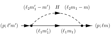
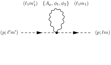
Refer to caption
Figure 1: One loop diagram for correction to KK masses of fermion with virtual gauge bosons including extra dimensional components.
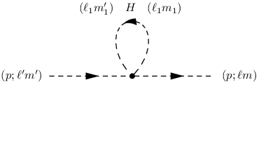
Refer to caption
Figure 2: One loop diagram for correction to KK masses of fermion with virtual Higgs bosons.

III.1 Correction to KK masses of fermion

The one loop diagrams relevant to correction to KK masses of fermion are given as Fig. 2 and 2 where corresponding quantum numbers {ℓ,m}\{\ell,m\} are shown for each external and internal lines. The Fig. 2 shows the virtual gauge boson contributions including both four-dimensional components and extra-dimensional components, and the Fig. 2 shows the virtual Higgs boson contribution. Here we discuss the one loop diagram Fig. 2 with virtual AμA_{\mu} for external Ψ+(±γ5)\Psi_{+}^{(\pm\gamma_{5})} case to show the structure of the quantum correction. We can calculate the diagram, by applying the propagators Eq. (33) and (36) and vertex Eq. (46), such that

−i​ΣFig​.1​(p,ℓ​m,ℓ′​m′)=\displaystyle-i\Sigma^{\rm Fig.1}(p;\ell m;\ell^{\prime}m^{\prime})= 14​R2​∑ℓ1=0ℓm​a​x∑ℓ2=0ℓm​a​x∑m1=−ℓ1ℓ1∑m1′=−ℓ1ℓ1∫Λd4​k(2​π)4\displaystyle\frac{1}{4R^{2}}\sum_{\ell_{1}=0}^{\ell_{max}}\sum_{\ell_{2}=0}^{\ell_{max}}\sum_{m_{1}=-\ell_{1}}^{\ell_{1}}\sum_{m_{1}^{\prime}=-\ell_{1}}^{\ell_{1}}\int_{\Lambda}\frac{d^{4}k}{(2\pi)^{4}}
×[−i(p−k)2−Mℓ22(δm1−m,m1′−m′+(−1)ℓ2δ−(m1−m),m1′−m′)\displaystyle\times\biggl[\frac{-i}{(p-k)^{2}-M^{2}_{\ell_{2}}}(\delta_{m_{1}-m,m_{1}^{\prime}-m^{\prime}}+(-1)^{\ell_{2}}\delta_{-(m_{1}-m),m_{1}^{\prime}-m^{\prime}})
×(i​g6​a​Ta​γμ)​[Iℓ1​m1′;ℓ2​m1′−m′;ℓ′​m′α​PR+Iℓ1​m1′;ℓ2​m1′−m′;ℓ′​m′β​PL]\displaystyle\quad\times(ig_{6a}T^{a}\gamma^{\mu})[I^{\alpha}_{\ell_{1}m_{1}^{\prime};\ell_{2}m_{1}^{\prime}-m^{\prime};\ell^{\prime}m^{\prime}}P_{R}+I^{\beta}_{\ell_{1}m_{1}^{\prime};\ell_{2}m_{1}^{\prime}-m^{\prime};\ell^{\prime}m^{\prime}}P_{L}]
×i/​k+i​γ5​Mℓ1​(δm1,m1′∓(−1)ℓ1+m1​δ−m1,m1′​γ5)\displaystyle\quad\times\frac{i}{\hbox to0.0pt{/\hss}k+i\gamma_{5}M_{\ell_{1}}}(\delta_{m_{1},m_{1}^{\prime}}\mp(-1)^{\ell_{1}+m_{1}}\delta_{-m_{1},m_{1}^{\prime}}\gamma_{5})
×(ig6​aTaγμ)[Iℓ​m;ℓ2​m1−m¯;ℓ1​m1αPR+Iℓ​m;ℓ2​m1−m¯;ℓ1​m1βPL]],\displaystyle\quad\times(ig_{6a}T^{a}\gamma_{\mu})[I^{\alpha}_{\ell m;\underline{\ell_{2}m_{1}-m};\ell_{1}m_{1}}P_{R}+I^{\beta}_{\ell m;\underline{\ell_{2}m_{1}-m};\ell_{1}m_{1}}P_{L}]\biggr], (47)

where PLP_{L} and PRP_{R} on the RHS will be interchanged for Ψ−(±γ5)\Psi_{-}^{(\pm\gamma_{5})} and the underline for the KK numbers in the vertex factor Iℓ​m;ℓ2​m1−m¯;ℓ1​m1α⁡(β)I^{\alpha(\beta)}_{\ell m;\underline{\ell_{2}m_{1}-m};\ell_{1}m_{1}} shows the corresponding spherical harmonics is conjugate one Yℓ2​m1−m∗Y^{*}_{\ell_{2}m_{1}-m}. The quantum numbers ℓ1\ell_{1}, ℓ2\ell_{2}, m1m_{1} and m1′m_{1}^{\prime} are associated with the KK modes in the loop which are summed over. In this paper we employ, for all one-loop diagram calculations, the cut-off Λ\Lambda for four momentum integration and ℓm​a​x\ell_{max} for angular momentum sum, in order to regularize the loop diagram. Summing over m1′m_{1}^{\prime}, the products of Kronecker delta and vertex factors IxI^{x} (x=αx=\alpha or β\beta) are arranged as

∑m1′(δm1−m,m1′−m′+(−1)ℓ2​δ−(m1−m),m1′−m′)​(δm1,m1′±(−1)ℓ1+m1​δ−m1,m1′​γ5)\displaystyle\sum_{m_{1}^{\prime}}(\delta_{m_{1}-m,m_{1}^{\prime}-m^{\prime}}+(-1)^{\ell_{2}}\delta_{-(m_{1}-m),m_{1}^{\prime}-m^{\prime}})(\delta_{m_{1},m_{1}^{\prime}}\pm(-1)^{\ell_{1}+m_{1}}\delta_{-m_{1},m_{1}^{\prime}}\gamma_{5})
×Iℓ1​m1′;ℓ2​m1′−m′;ℓ′​m′x​Iℓ​m;ℓ2​m1−m¯;ℓ1​m1x′\displaystyle\qquad\times I^{x}_{\ell_{1}m_{1}^{\prime};\ell_{2}m_{1}^{\prime}-m^{\prime};\ell^{\prime}m^{\prime}}I^{x^{\prime}}_{\ell m;\underline{\ell_{2}m_{1}-m};\ell_{1}m_{1}}
=(δm,m′±(−1)ℓ′+m​δ−m,m′​γ5)​Iℓ1​m1;ℓ2​m1−m;ℓ′​mx​Iℓ​m;ℓ2​m−m1;ℓ1​m1x′\displaystyle=(\delta_{m,m^{\prime}}\pm(-1)^{\ell^{\prime}+m}\delta_{-m,m^{\prime}}\gamma_{5})I^{x}_{\ell_{1}m_{1};\ell_{2}m_{1}-m;\ell^{\prime}m}I^{x^{\prime}}_{\ell m;\ell_{2}m-m_{1};\ell_{1}m_{1}}
+(−1)ℓ2​(δ2​m1,m+m′±(−1)ℓ′+m​δ2​m1,m−m′​γ5)​Iℓ1​m1;ℓ2−m1+m;ℓ′​2​m1−mx​Iℓ​m;ℓ2​m−m1;ℓ1​m1x′,\displaystyle\quad+(-1)^{\ell_{2}}(\delta_{2m_{1},m+m^{\prime}}\pm(-1)^{\ell^{\prime}+m}\delta_{2m_{1},m-m^{\prime}}\gamma_{5})I^{x}_{\ell_{1}m_{1};\ell_{2}-m_{1}+m;\ell^{\prime}2m_{1}-m}I^{x^{\prime}}_{\ell m;\ell_{2}m-m_{1};\ell_{1}m_{1}}, (48)

where we used the relation Iℓ1−m1;ℓ2−m2;ℓ3−m3x=(−1)ℓ1+ℓ2+ℓ3+m1+m3​Iℓ1​m1;ℓ2​m2;ℓ3​m3xI^{x}_{\ell_{1}-m_{1};\ell_{2}-m_{2};\ell_{3}-m_{3}}=(-1)^{\ell_{1}+\ell_{2}+\ell_{3}+m_{1}+m_{3}}I^{x}_{\ell_{1}m_{1};\ell_{2}m_{2};\ell_{3}m_{3}} obtained from the definition of the vertex factor given in Eq. (46). The first term in RHS of Eq. (48) corresponds to bulk contribution conserving KK-number mm, and the second term corresponds to the boundary contribution violating the conservation of the KK-number mm. Thus the one-loop diagram contribution can be separated to the bulk and boundary contributions such that

−i​ΣFig​.1​(p,μ,ℓ​m,ℓ′​m′)=\displaystyle-i\Sigma^{\rm Fig.1}(p;\mu;\ell m;\ell^{\prime}m^{\prime})= −i​ΣbulkFig​.1​(p,ℓ​m,ℓ′​m′)−i​ΣboundFig​.1​(μ,ℓ​m,ℓ′​m′)\displaystyle-i\Sigma^{\rm Fig.1}_{\rm bulk}(p;\ell m;\ell^{\prime}m^{\prime})-i\Sigma^{\rm Fig.1}_{\rm bound}(\mu;\ell m;\ell^{\prime}m^{\prime}) (49)

where bulk contribution is proportional to mm conserving Kronecker deltas {δm,m′,δ−m,m′}\{\delta_{m,m^{\prime}},\delta_{-m,m^{\prime}}\}, and the boundary contribution is proportional to mm violating Kronecker deltas {δ2​m1,m+m′,δ2​m1,m−m′}\{\delta_{2m_{1},m+m^{\prime}},\delta_{2m_{1},m-m^{\prime}}\}. As usual we combine denominator in the momentum integral using Feynman parameter α\alpha, and carry out Wick rotation. The momentum integral becomes

∫Λd4​k(2​π)4​1[(p−k)2−Mℓ22]​[k2−Mℓ12]=i(4​π)2​∫01d​α​∫0Λ2kE2​d​kE2[kE2−α⁡(1−α)​p2+Mℓ12​(1−α)+Mℓ22​α]2\displaystyle\int_{\Lambda}\frac{d^{4}k}{(2\pi)^{4}}\frac{1}{[(p-k)^{2}-M^{2}_{\ell_{2}}][k^{2}-M_{\ell_{1}}^{2}]}=\frac{i}{(4\pi)^{2}}\int_{0}^{1}d\alpha\int_{0}^{\Lambda^{2}}\frac{k_{E}^{2}dk_{E}^{2}}{[k_{E}^{2}-\alpha(1-\alpha)p^{2}+M_{\ell_{1}}^{2}(1-\alpha)+M_{\ell_{2}}^{2}\alpha]^{2}} (50)

where we performed the substitution k−α​p→kk-\alpha p\to k, kEk_{E} is a Euclidean 4-momentum, and the integration over kE2k_{E}^{2} is regularized by cut-off Λ\Lambda. We estimate the momentum integration numerically taking cut-off Λ\Lambda as parameter for bulk contribution, while we only left leading log-divergent part with renormalization scale μ\mu for boundary contribution such that

∫0Λ2kE2​d​kE2[kE2−α⁡(1−α)​p2+Mℓ12​(1−α)+Mℓ22​α]2→log⁡(Λ2μ2),\int_{0}^{\Lambda^{2}}\frac{k_{E}^{2}dk_{E}^{2}}{[k_{E}^{2}-\alpha(1-\alpha)p^{2}+M_{\ell_{1}}^{2}(1-\alpha)+M_{\ell_{2}}^{2}\alpha]^{2}}\rightarrow\log\Bigl(\frac{\Lambda^{2}}{\mu^{2}}\Bigr), (51)

assuming vanishing contribution at the cut-off scale Λ\Lambda. Then after arranging the terms, Eq. (47) is organized as

−i​ΣbulkFig​.1​(p,ℓ​m,ℓ′​m′)=\displaystyle-i\Sigma_{\rm bulk}^{\rm Fig.1}(p;\ell m;\ell^{\prime}m^{\prime})= [/p(iΣbulkFig​.1,L(p;ℓm;ℓ′m′)PL+iΣbulkFig​.1,R(p;ℓm;ℓ′m′)PR)\displaystyle\Bigl[\hbox to0.0pt{/\hss}p(i\Sigma_{\rm bulk}^{{\rm Fig.1},L}(p;\ell m;\ell^{\prime}m^{\prime})P_{L}+i\Sigma_{\rm bulk}^{{\rm Fig.1},R}(p;\ell m;\ell^{\prime}m^{\prime})P_{R})
+iγ5(iΣ~bulkFig​.1,L(p;ℓm;ℓ′m′)PL+iΣ~bulkFig​.1,R(p;ℓm;ℓ′m′)PR)]\displaystyle+i\gamma_{5}(i\tilde{\Sigma}_{\rm bulk}^{{\rm Fig.1},L}(p;\ell m;\ell^{\prime}m^{\prime})P_{L}+i\tilde{\Sigma}_{\rm bulk}^{{\rm Fig.1},R}(p;\ell m;\ell^{\prime}m^{\prime})P_{R})\Bigr] (52)
−i​ΣboundFig​.1​(p,ℓ​m,ℓ′​m′)=\displaystyle-i\Sigma_{\rm bound}^{\rm Fig.1}(p;\ell m;\ell^{\prime}m^{\prime})= [/p(iΣboundFig​.1,L(μ;ℓm;ℓ′m′)PL+iΣboundFig​.1,R(μ;ℓm;ℓ′m′)PR)\displaystyle\Bigl[\hbox to0.0pt{/\hss}p(i\Sigma_{\rm bound}^{{\rm Fig.1},L}(\mu;\ell m;\ell^{\prime}m^{\prime})P_{L}+i\Sigma_{\rm bound}^{{\rm Fig.1},R}(\mu;\ell m;\ell^{\prime}m^{\prime})P_{R})
+iγ5(iΣ~boundFig​.1,L(μ;ℓm;ℓ′m′)PL+iΣ~boundFig​.1,R(μ;ℓm;ℓ′m′)PR)],\displaystyle+i\gamma_{5}(i\tilde{\Sigma}_{\rm bound}^{{\rm Fig.1},L}(\mu;\ell m;\ell^{\prime}m^{\prime})P_{L}+i\tilde{\Sigma}_{\rm bound}^{{\rm Fig.1},R}(\mu;\ell m;\ell^{\prime}m^{\prime})P_{R})\Bigr], (53)

where the coefficients ΣL⁡(R)\Sigma^{L(R)} and Σ~L⁡(R)\tilde{\Sigma}^{L(R)} correspond to the terms proportional to /​p\hbox to0.0pt{/\hss}p and i​γ5i\gamma_{5} respectively, associated with PL⁡(R)P_{L(R)}. These coefficients are explicitly given by

i​ΣbulkFig​.1,L⁡(R)​(p,ℓ​m,ℓ′​m′)\displaystyle i\Sigma_{\rm bulk}^{{\rm Fig.1},L(R)}(p;\ell m;\ell^{\prime}m^{\prime}) =i​g6​a264​π2​R2​(Ta)2​∑ℓ1=0ℓm​a​x∑ℓ2=0ℓm​a​x∑m1=−ℓ1ℓ1∫01d​α​∫0Λ2x​d​x[x+Δ]2​(−1)m1−m\displaystyle=i\frac{g_{6a}^{2}}{64\pi^{2}R^{2}}(T^{a})^{2}\sum_{\ell_{1}=0}^{\ell_{max}}\sum_{\ell_{2}=0}^{\ell_{max}}\sum_{m_{1}=-\ell_{1}}^{\ell_{1}}\int_{0}^{1}d\alpha\int^{\Lambda^{2}}_{0}\frac{xdx}{[x+\Delta]^{2}}(-1)^{m_{1}-m}
×2​α​Iℓ1​m1;ℓ2​m1−m;ℓ′​mβ⁡(α)​Iℓ​m;ℓ2​m−m1;ℓ1​m1β⁡(α)​(δm,m′±(−1)ℓ′+m​δ−m,m′​γ5),\displaystyle\quad\times 2\alpha I^{\beta(\alpha)}_{\ell_{1}m_{1};\ell_{2}m_{1}-m;\ell^{\prime}m}I^{\beta(\alpha)}_{\ell m;\ell_{2}m-m_{1};\ell_{1}m_{1}}\bigl(\delta_{m,m^{\prime}}\pm(-1)^{\ell^{\prime}+m}\delta_{-m,m^{\prime}}\gamma_{5}\bigr), (54)
i​Σ~bulkFig​.1,L⁡(R)​(p,ℓ​m,ℓ′​m′)\displaystyle i\tilde{\Sigma}_{\rm bulk}^{{\rm Fig.1},L(R)}(p;\ell m;\ell^{\prime}m^{\prime}) =i​g6​a264​π2​R2​(Ta)2​∑ℓ1=0ℓm​a​x∑ℓ2=0ℓm​a​x∑m1=−ℓ1ℓ1∫01d​α​∫0Λ2x​d​x[x+Δ]2​(−1)m1−m\displaystyle=i\frac{g_{6a}^{2}}{64\pi^{2}R^{2}}(T^{a})^{2}\sum_{\ell_{1}=0}^{\ell_{max}}\sum_{\ell_{2}=0}^{\ell_{max}}\sum_{m_{1}=-\ell_{1}}^{\ell_{1}}\int_{0}^{1}d\alpha\int^{\Lambda^{2}}_{0}\frac{xdx}{[x+\Delta]^{2}}(-1)^{m_{1}-m}
×4​Mℓ1​Iℓ1​m1;ℓ2​m1−m;ℓ′​mα⁡(β)​Iℓ​m;ℓ2​m−m1;ℓ1​m1β⁡(α)​(δm,m′±(−1)ℓ′+m​δ−m,m′​γ5),\displaystyle\quad\times 4M_{\ell_{1}}I^{\alpha(\beta)}_{\ell_{1}m_{1};\ell_{2}m_{1}-m;\ell^{\prime}m}I^{\beta(\alpha)}_{\ell m;\ell_{2}m-m_{1};\ell_{1}m_{1}}\bigl(\delta_{m,m^{\prime}}\pm(-1)^{\ell^{\prime}+m}\delta_{-m,m^{\prime}}\gamma_{5}\bigr), (55)
i​ΣboundFig​.1,L⁡(R)​(μ,ℓ​m,ℓ′​m′)\displaystyle i\Sigma_{\rm bound}^{{\rm Fig.1},L(R)}(\mu;\ell m;\ell^{\prime}m^{\prime}) =i​g6​a264​π2​R2​(Ta)2​∑ℓ1=0ℓm​a​x∑ℓ2=0ℓm​a​x∑m1=−ℓ1ℓ1(−1)m1−m+ℓ2​log⁡(Λ2μ2)\displaystyle=i\frac{g_{6a}^{2}}{64\pi^{2}R^{2}}(T^{a})^{2}\sum_{\ell_{1}=0}^{\ell_{max}}\sum_{\ell_{2}=0}^{\ell_{max}}\sum_{m_{1}=-\ell_{1}}^{\ell_{1}}(-1)^{m_{1}-m+\ell_{2}}\log\Bigl(\frac{\Lambda^{2}}{\mu^{2}}\Bigr)
×Iℓ1​m1;ℓ2−m1+m;ℓ′​2​m1−mβ⁡(α)​Iℓ​m;ℓ2​m−m1;ℓ1​m1β⁡(α)\displaystyle\quad\times I^{\beta(\alpha)}_{\ell_{1}m_{1};\ell_{2}-m_{1}+m;\ell^{\prime}2m_{1}-m}I^{\beta(\alpha)}_{\ell m;\ell_{2}m-m_{1};\ell_{1}m_{1}}\
×(δ2​m1,m+m′±(−1)ℓ′+m​δ2​m1,m−m′​γ5),\displaystyle\quad\times\bigl(\delta_{2m_{1},m+m^{\prime}}\pm(-1)^{\ell^{\prime}+m}\delta_{2m_{1},m-m^{\prime}}\gamma_{5}\bigr), (56)
i​Σ~boundFig​.1,L⁡(R)​(μ,ℓ​m,ℓ′​m′)\displaystyle i\tilde{\Sigma}_{\rm bound}^{{\rm Fig.1},L(R)}(\mu;\ell m;\ell^{\prime}m^{\prime}) =i​g6​a264​π2​R2​(Ta)2​∑ℓ1=0ℓm​a​x∑ℓ2=0ℓm​a​x∑m1=−ℓ1ℓ1(−1)m1−m+ℓ2​log⁡(Λ2μ2)\displaystyle=i\frac{g_{6a}^{2}}{64\pi^{2}R^{2}}(T^{a})^{2}\sum_{\ell_{1}=0}^{\ell_{max}}\sum_{\ell_{2}=0}^{\ell_{max}}\sum_{m_{1}=-\ell_{1}}^{\ell_{1}}(-1)^{m_{1}-m+\ell_{2}}\log\Bigl(\frac{\Lambda^{2}}{\mu^{2}}\Bigr)
×4​Mℓ1​Iℓ1​m1;ℓ2−m1+m;ℓ′​2​m1−mα⁡(β)​Iℓ​m;ℓ2​m−m1;ℓ1​m1β⁡(α)\displaystyle\quad\times 4M_{\ell_{1}}I^{\alpha(\beta)}_{\ell_{1}m_{1};\ell_{2}-m_{1}+m;\ell^{\prime}2m_{1}-m}I^{\beta(\alpha)}_{\ell m;\ell_{2}m-m_{1};\ell_{1}m_{1}}
×(δ2​m1,m+m′±(−1)ℓ′+m​δ2​m1,m−m′​γ5),\displaystyle\quad\times\bigl(\delta_{2m_{1},m+m^{\prime}}\pm(-1)^{\ell^{\prime}+m}\delta_{2m_{1},m-m^{\prime}}\gamma_{5}\bigr), (57)

where Δ=−α⁡(1−α)​p2+(1−α)​Mℓ12+α​Mℓ22\Delta=-\alpha(1-\alpha)p^{2}+(1-\alpha)M_{\ell_{1}}^{2}+\alpha M_{\ell_{2}}^{2}. We also note that there appear sign factors of (−1){ℓ,m}(-1)^{\{\ell,m\}} from propagators in S2/Z2S^{2}/Z_{2} orbifold and vertices, which lead different sign contributions from each KK modes in the loop. Then the contributions depend on ℓm​a​x\ell_{max} differently for even or odd ℓm​a​x\ell_{max} as we will see below. Also we can numerically check that external ℓ\ell and mm are conserved so that ℓ=ℓ′\ell=\ell^{\prime} and m=m′m=m^{\prime} cases give non-zero contribution, which is satisfied for other diagrams. The other diagrams are also calculated in the same manner, and we list the contributions from each diagrams in Table 9. Therefore we obtain one-loop level correction to the Lagrangian such that

δ​L1−loop=\displaystyle\delta L_{\rm 1-loop}= ΣbulkL​(p2,ℓ​m,ℓ​m)​ψ¯ℓ​m​L​i​γμ​∂μψℓ​m​L+ΣbulkR​(p2,ℓ​m,ℓ​m)​ψ¯ℓ​m​R​i​γμ​∂μψℓ​m​R\displaystyle\Sigma_{\rm bulk}^{L}(p^{2};\ell m;\ell m)\bar{\psi}_{\ell mL}i\gamma^{\mu}\partial_{\mu}\psi_{\ell mL}+\Sigma_{\rm bulk}^{R}(p^{2};\ell m;\ell m)\bar{\psi}_{\ell mR}i\gamma^{\mu}\partial_{\mu}\psi_{\ell mR}
+12[Σ~b​u​l​kL(p2;ℓm;ℓm)+Σ~b​u​l​kR(p2;ℓm;ℓm)]ψ¯ℓ​miγ5ψℓ​m]\displaystyle+\frac{1}{2}\Bigl[\tilde{\Sigma}_{bulk}^{L}(p^{2};\ell m;\ell m)+\tilde{\Sigma}_{bulk}^{R}(p^{2};\ell m;\ell m)]\bar{\psi}_{\ell m}i\gamma_{5}\psi_{\ell m}\Bigr]
+ΣboundL(μ;ℓm;ℓm)ψ¯ℓ​m​Liγμ∂μψℓ​m​L+ΣboundR(μ;ℓm;ℓm)ψ¯ℓ​m​Riγμ∂μψℓ​m​R\displaystyle+\Sigma_{\rm bound}^{L}(\mu;\ell m;\ell m)\bar{\psi}_{\ell mL}i\gamma^{\mu}\partial_{\mu}\psi_{\ell mL}+\Sigma_{\rm bound}^{R}(\mu;\ell m;\ell m)\bar{\psi}_{\ell mR}i\gamma^{\mu}\partial_{\mu}\psi_{\ell mR}
+12[Σ~boundL(μ;ℓm;ℓm)+Σ~boundR(μ;ℓm;ℓm)]ψ¯ℓ​miγ5ψℓ​m],\displaystyle+\frac{1}{2}\Bigl[\tilde{\Sigma}_{\rm bound}^{L}(\mu;\ell m;\ell m)+\tilde{\Sigma}_{\rm bound}^{R}(\mu;\ell m;\ell m)]\bar{\psi}_{\ell m}i\gamma_{5}\psi_{\ell m}\Bigr], (58)

where each coefficients ΣbulkL⁡(R)\Sigma^{L(R)}_{\rm bulk}, ΣboundL⁡(R)\Sigma^{L(R)}_{\rm bound}, Σ~bulkL⁡(R)\tilde{\Sigma}^{L(R)}_{\rm bulk} and Σ~boundL⁡(R)\tilde{\Sigma}^{L(R)}_{\rm bound} are understood as the sum of corresponding contributions from all diagrams.
To obtain one-loop corrections to KK mass, we take into account a renormalization condition for each KK modes. The kinetic and KK mass terms of each KK modes of fermion are given in Eq. (14). Defining as a renormalization of fields, ψR⁡(L)→ZR⁡(L)​ψR⁡(L)=1+δR⁡(L)​ψR⁡(L)\psi_{R(L)}\rightarrow\sqrt{Z_{R(L)}}\psi_{R(L)}=\sqrt{1+\delta_{R(L)}}\psi_{R(L)}, the terms in Eq. (14) become

ψ¯L​ℓ​m​i​γμ​∂μψL​ℓ​m+ψ¯R​ℓ​m​i​γμ​∂μψR​ℓ​m+i​Mℓ​ψ¯L​ℓ​m​γ5​ψR​ℓ​m+i​Mℓ​ψ¯R​ℓ​m​γ5​ψL​ℓ​m\displaystyle\bar{\psi}_{L\ell m}i\gamma^{\mu}\partial_{\mu}\psi_{L\ell m}+\bar{\psi}_{R\ell m}i\gamma^{\mu}\partial_{\mu}\psi_{R\ell m}+iM_{\ell}\bar{\psi}_{L\ell m}\gamma_{5}\psi_{R\ell m}+iM_{\ell}\bar{\psi}_{R\ell m}\gamma_{5}\psi_{L\ell m}
δL​ψ¯L​ℓ​m​i​γμ​∂μψL​ℓ​m+δR​ψ¯R​ℓ​m​i​γμ​∂μψR​ℓ​m+12​(δL+δR)​(i​Mℓ​ψ¯L​ℓ​m​γ5​ψR​ℓ​m+i​Mℓ​ψ¯R​ℓ​m​γ5​ψL​ℓ​m),\displaystyle\delta_{L}\bar{\psi}_{L\ell m}i\gamma^{\mu}\partial_{\mu}\psi_{L\ell m}+\delta_{R}\bar{\psi}_{R\ell m}i\gamma^{\mu}\partial_{\mu}\psi_{R\ell m}+\frac{1}{2}(\delta_{L}+\delta_{R})(iM_{\ell}\bar{\psi}_{L\ell m}\gamma_{5}\psi_{R\ell m}+iM_{\ell}\bar{\psi}_{R\ell m}\gamma_{5}\psi_{L\ell m}), (59)

where we have taken up to the first order in δR⁡(L)\delta_{R(L)}, which corresponds to the counter terms. Thus the contribution from these counter terms is shown by

conterterms⁡(p,ℓ​m)=i​/​p​[δL​PL+δR​PR]+i⁡(i​γ5​Mℓ)​(PL+PR)​12​[δL+δR].{\rm conterterms}(p;\ell m)=i\hbox to0.0pt{/\hss}p[\delta_{L}P_{L}+\delta_{R}P_{R}]+i(i\gamma_{5}M_{\ell})(P_{L}+P_{R})\frac{1}{2}[\delta_{L}+\delta_{R}]. (60)

Then we employ the renormalization conditions at a cut off scale Λ\Lambda as

(i​δL+i​Σb​u​l​kL​(p2,ℓ​m,ℓ​m))∣p2=−Λ2,Mℓ​m​a​x2=Λ2=0,\displaystyle\bigl(i\delta_{L}+i\Sigma_{bulk}^{L}(p^{2};\ell m;\ell m))\mid_{p^{2}=-\Lambda^{2},M_{\ell max}^{2}=\Lambda^{2}}=0, (61)
(i​δR+i​Σb​u​l​kR​(p2,ℓ​m,ℓ​m))∣p2=−Λ2,Mℓ​m​a​x2=Λ2=0,\displaystyle\bigl(i\delta_{R}+i\Sigma_{bulk}^{R}(p^{2};\ell m;\ell m))\mid_{p^{2}=-\Lambda^{2},M_{\ell max}^{2}=\Lambda^{2}}=0, (62)

which corresponds to the requirement that the kinetic term has canonical form at the cut-off scale, and the counter terms δR⁡(L)\delta_{R(L)} are determined from these conditions. Combining contributions from the one-loop diagrams and the counter terms, we obtain the corrected kinetic and KK mass terms such that

δ​L=\displaystyle\delta L= δL​ψ¯L​ℓ​m​i​γμ​∂μψL​ℓ​m+δR​ψ¯R​ℓ​m​i​γμ​∂μψR​ℓ​m\displaystyle\delta_{L}\bar{\psi}_{L\ell m}i\gamma^{\mu}\partial_{\mu}\psi_{L\ell m}+\delta_{R}\bar{\psi}_{R\ell m}i\gamma^{\mu}\partial_{\mu}\psi_{R\ell m}
+12​(δL+δR)​(ψ¯L​ℓ​m​i​Mℓ​γ5​ψR​ℓ​m+ψ¯R​ℓ​m​i​Mℓ​γ5​ψL​ℓ​m)+δ​L1−loop.\displaystyle+\frac{1}{2}(\delta_{L}+\delta_{R})(\bar{\psi}_{L\ell m}iM_{\ell}\gamma_{5}\psi_{R\ell m}+\bar{\psi}_{R\ell m}iM_{\ell}\gamma_{5}\psi_{L\ell m})+\delta L_{\rm 1-loop}. (63)

Therefore, normalizing the kinetic terms by

ψR⁡(L)​ℓ​m→(1+ΣbulkR⁡(L)​(p2,ℓ​m,ℓ​m)+ΣboundR⁡(L)​(μ,ℓ​m,ℓ​m)+δR⁡(L))−12​ψR⁡(L)​ℓ​m,\psi_{R(L)\ell m}\rightarrow\left(1+\Sigma_{\rm bulk}^{R(L)}(p^{2};\ell m;\ell m)+\Sigma_{\rm bound}^{R(L)}(\mu;\ell m;\ell m)+\delta_{R(L)}\right)^{-\frac{1}{2}}\psi_{R(L)\ell m}, (64)

we obtain the corrected KK mass of

M~ℓ​m≃\displaystyle\tilde{M}_{\ell m}\simeq Mℓ+12​[(Σ~bulkL+Σ~bulkR)​(p2,ℓ​m,ℓ​m)+(Σ~boundL+Σ~boundR)​(μ,ℓ​m,ℓ​m)]\displaystyle M_{\ell}+\frac{1}{2}\left[(\tilde{\Sigma}^{L}_{\rm bulk}+\tilde{\Sigma}^{R}_{\rm bulk})(p^{2};\ell m;\ell m)+(\tilde{\Sigma}^{L}_{\rm bound}+\tilde{\Sigma}^{R}_{\rm bound})(\mu;\ell m;\ell m)\right]
−12​Mℓ​[(ΣbulkL+ΣbulkR)​(p2,ℓ​m,ℓ​m)+(ΣboundL+ΣboundR)​(μ,ℓ​m,ℓ​m)]\displaystyle-\frac{1}{2}M_{\ell}\Bigl[(\Sigma^{L}_{\rm bulk}+\Sigma^{R}_{\rm bulk})(p^{2};\ell m;\ell m)+(\Sigma^{L}_{\rm bound}+\Sigma^{R}_{\rm bound})(\mu;\ell m;\ell m)\Bigr]
≡\displaystyle\equiv Mℓ+(δ​M)ℓ​mψ\displaystyle M_{\ell}+(\delta M)^{\psi}_{\ell m} (65)

for each KK modes of fermions, where we have taken the first order of Σ\Sigma and δ\delta in RHS.

Refer to caption
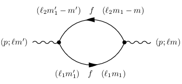
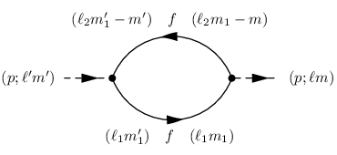
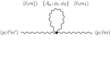
Figure 3: One loop diagram for correction to KK masses of gauge bosons {Aμ,ϕ1,ϕ2}\{A_{\mu},\phi_{1},\phi_{2}\} with virtual fermions.
Refer to caption
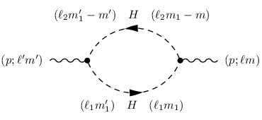
Figure 4: One loop diagram for correction to KK masses of gauge bosons {Aμ,ϕ1,ϕ2}\{A_{\mu},\phi_{1},\phi_{2}\} with virtual Higgs bosons.
Refer to caption
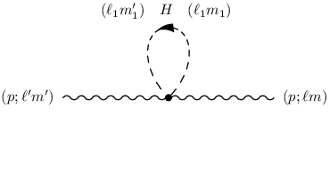
Figure 5: One loop diagram for correction to KK masses of gauge bosons {Aμ,ϕ1,ϕ2}\{A_{\mu},\phi_{1},\phi_{2}\} with virtual Higgs bosons.
Refer to caption
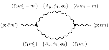
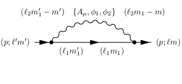
Figure 6: One loop diagram for correction to KK masses of gauge bosons {Aμ,ϕ1,ϕ2}\{A_{\mu},\phi_{1},\phi_{2}\} with virtual gauge bosons including extra components.

III.2 Correction to KK masses of gauge boson

The one loop diagrams corresponding to correction to KK masses of gauge bosons are given in Fig. 4-7 for both four-dimensional components and extra-dimensional components in external line, where corresponding quantum numbers {ℓ,m}\{\ell,m\} are shown for each external and internal lines. The Fig. 4 shows the fermion loop, the Fig. 4 and 6 show Higgs boson loops from 3-point and 4-point gauge interactions respectively, and the Fig. 6 and 7 show the gauge boson loops from 3-point and 4-point self-interactions respectively. These diagrams are calculated in the same manner as the case of KK mass of fermions, and we summarize the results in Appendix B. Separating bulk and boundary contributions, we can organize the one loop diagram contributions generally as

i​Πμ​ν​(p2,μ,ℓ​m,ℓ​m)=i​Πμ​νbulk​(p2,ℓ​m,ℓ​m)+i​Πμ​νbound​(p2,μ,ℓ​m,ℓ​m),\displaystyle i\Pi_{\mu\nu}(p^{2};\mu;\ell m;\ell m)=i\Pi_{\mu\nu}^{\rm bulk}(p^{2};\ell m;\ell m)+i\Pi_{\mu\nu}^{\rm bound}(p^{2};\mu;\ell m;\ell m), (66)
i​Πμ​νbulk⁡(bound)​(p2​(p2,μ),ℓ​m,ℓ​m)=(p2​gμ​ν−pμ​pν)​i​Πbulk⁡(bound)​(p2​(p2,μ),ℓ​m,ℓ​m)\displaystyle i\Pi_{\mu\nu}^{\rm bulk(bound)}(p^{2}(p^{2};\mu);\ell m;\ell m)=(p^{2}g_{\mu\nu}-p_{\mu}p_{\nu})i\Pi_{\rm bulk(bound)}(p^{2}(p^{2};\mu);\ell m;\ell m)
+gμ​ν​i​Π~bulk⁡(bound)​(p2​(p2,μ),ℓ​m,ℓ​m),\displaystyle\hskip 156.49014pt+g_{\mu\nu}i\tilde{\Pi}_{\rm bulk(bound)}(p^{2}(p^{2};\mu);\ell m;\ell m), (67)

where we also separated the terms proportional to (p2​gμ​ν−pμ​pν)(p^{2}g_{\mu\nu}-p_{\mu}p_{\nu}) contributing the correction of kinetic term of AμA_{\mu} and the terms proportional to gμ​νg_{\mu\nu} in RHS of second line. The contributions to the coefficients Π⁡(Π~)\Pi(\tilde{\Pi})s from each diagrams are summarized in Table 10 and 11. Thus the correction to the Lagrangian is

δ​L1​l​o​o​p=\displaystyle\delta L_{\rm 1loop}= 14​Πbulk​(p2,ℓ​m,ℓ​m)​Fl​mμ​ν​Fℓ​m​μ​ν+12​Π~bulk​(p2,ℓ​m,ℓ​m)​Aℓ​mμ​Aℓ​m​μ\displaystyle\frac{1}{4}\Pi_{\rm bulk}(p^{2};\ell m;\ell m)F^{\mu\nu}_{lm}F_{\ell m\mu\nu}+\frac{1}{2}\tilde{\Pi}_{\rm bulk}(p^{2};\ell m;\ell m)A^{\mu}_{\ell m}A_{\ell m\mu}
+14​Πbound​(p2,μ,ℓ​m,ℓ​m)​Fl​mμ​ν​Fℓ​m​μ​ν+12​Π~bound​(p2,μ,ℓ​m,ℓ​m)​Aℓ​mμ​Aℓ​m​μ\displaystyle+\frac{1}{4}\Pi_{\rm bound}(p^{2};\mu;\ell m;\ell m)F^{\mu\nu}_{lm}F_{\ell m\mu\nu}+\frac{1}{2}\tilde{\Pi}_{\rm bound}(p^{2};\mu;\ell m;\ell m)A^{\mu}_{\ell m}A_{\ell m\mu} (68)

where Π⁡(Π~)\Pi(\tilde{\Pi})s in the RHS are understood as the sum of corresponding contributions from all diagrams.

Refer to caption
Figure 7: One loop diagram for correction to KK masses of gauge bosons {Aμ,ϕ1,ϕ2}\{A_{\mu},\phi_{1},\phi_{2}\} with virtual gauge bosons including extra components.

As in the fermion case, we consider the renormalization condition to obtain one-loop corrections to KK masses for KK gauge bosons. The kinetic and KK mass terms of each KK modes of gauge boson are given in Eq. (18). Defining as a renormalization of gauge field, Aμ→Z3​Aμ=1+δ3​AμA_{\mu}\rightarrow\sqrt{Z_{3}}A_{\mu}=\sqrt{1+\delta_{3}}A_{\mu}, these terms become

−14​Fℓ​mμ​ν​Fℓ​m​μ​ν+12​Mℓ2​Aℓ​mμ​Aℓ​m​μ−14​δ3​Fℓ​mμ​ν​Fℓ​m​μ​ν+12​δ3​Mℓ2​Aℓ​mμ​Aℓ​m​μ,-\frac{1}{4}F^{\mu\nu}_{\ell m}F_{\ell m\mu\nu}+\frac{1}{2}M_{\ell}^{2}A^{\mu}_{\ell m}A_{\ell m\mu}-\frac{1}{4}\delta_{3}F^{\mu\nu}_{\ell m}F_{\ell m\mu\nu}+\frac{1}{2}\delta_{3}M_{\ell}^{2}A^{\mu}_{\ell m}A_{\ell m\mu}, (69)

where we have taken up to the first order in δ3\delta_{3} corresponding to counter terms. Thus the contribution from these counter terms is

counterterm⁡(p2,ℓ​m)=−i⁡(p2​gμ​ν−pμ​pν)​δ3+i​Mℓ2​δ3.{\rm counterterm}(p^{2};\ell m)=-i(p^{2}g_{\mu\nu}-p_{\mu}p_{\nu})\delta_{3}+iM_{\ell}^{2}\delta_{3}. (70)

Then we employ the renormalization condition at a cut-off scale Λ\Lambda as

(Πb​u​l​k​(p2,ℓ​m,ℓ​m)−δ3)∣p2=−Λ2,Mℓ​m​a​x2=Λ2=0(\Pi_{bulk}(p^{2};\ell m;\ell m)-\delta_{3})\mid_{p^{2}=-\Lambda^{2},M_{\ell max}^{2}=\Lambda^{2}}=0 (71)

which requires the canonical form of kinetic term at the cut-off scale as in the fermion case, and the counter term δ3\delta_{3} is determined by the condition. Combining contributions from one-loop diagrams and counter terms, we obtain the one-loop corrections to kinetic and KK mass terms such that

δ​L=−14​δ3​Fℓ​mμ​ν​Fℓ​m​μ​ν+12​δ3​Aℓ​mμ​L^2​Aℓ​m​μ+δ​L1−loop.\displaystyle\delta L=-\frac{1}{4}\delta_{3}F^{\mu\nu}_{\ell m}F_{\ell m\mu\nu}+\frac{1}{2}\delta_{3}A^{\mu}_{\ell m}\hat{L}^{2}A_{\ell m\mu}+\delta L_{\rm 1-loop}. (72)

Therefore, normalizing the kinetic terms by

Aℓ​mμ→(1−Πbulk​(p2,ℓ​m,ℓ​m)−Πb​o​u​n​d​(p2,μ,ℓ​m,ℓ​m)+δ3)−12​Aℓ​mμ,A^{\mu}_{\ell m}\rightarrow\left(1-\Pi_{\rm bulk}(p^{2};\ell m;\ell m)-\Pi_{bound}(p^{2};\mu;\ell m;\ell m)+\delta_{3}\right)^{-\frac{1}{2}}A^{\mu}_{\ell m}, (73)

we obtain one-loop corrections to KK mass

M~ℓ2=\displaystyle\tilde{M}_{\ell}^{2}= Mℓ2+Π~bulk​(p2,ℓ​m,ℓ​m)+Π~bound​(p2,μ,ℓ​m,ℓ​m)+Mℓ2​[Πbulk​(p2,ℓ​m,ℓ​m)+Πbound​(p2,μ,ℓ​m,ℓ​m)],\displaystyle M_{\ell}^{2}+\tilde{\Pi}_{\rm bulk}(p^{2};\ell m;\ell m)+\tilde{\Pi}_{\rm bound}(p^{2};\mu;\ell m;\ell m)+M_{\ell}^{2}\bigl[\Pi_{\rm bulk}(p^{2};\ell m;\ell m)+\Pi_{\rm bound}(p^{2};\mu;\ell m;\ell m)\bigr],
≡\displaystyle\equiv Mℓ2+(δ​M2)ℓ​mAμ,\displaystyle M_{\ell}^{2}+(\delta M^{2})^{A_{\mu}}_{\ell m}, (74)

for each KK modes of gauge bosons, where we have taken the first order in Π\Pi and δ3\delta_{3} in RHS.

The extra dimensional components of gauge fields Aθ,ϕA_{\theta,\phi} are considered as scalar fields in four dimensions, and the KK mass eigenstates are given by ϕi\phi_{i} which are defined as Eq. (20) and (21). Then the kinetic and KK mass term of ϕi\phi_{i} are the same form as that of scalar field. For ϕi\phi_{i}, we write the contributions from one-loop diagrams to corrections of diagonal mass terms ϕi​ϕi\phi_{i}\phi_{i} such that

i​Θ(i)​(p2,μ,ℓ​m,ℓ​m′)=i​Θbulk(i)​(p2,μ,ℓ​m,ℓ​m′)+i​Θbound(i)​(p2,μ,ℓ​m,ℓ​m′),\displaystyle i\Theta^{(i)}(p^{2};\mu;\ell m;\ell m^{\prime})=i\Theta^{(i)}_{\rm bulk}(p^{2};\mu;\ell m;\ell m^{\prime})+i\Theta^{(i)}_{\rm bound}(p^{2};\mu;\ell m;\ell m^{\prime}), (75)
i​Θbulk⁡(bound)(i)​(p2​(p2,μ),ℓ​m,ℓ​m′)=p2​i​Θbulk⁡(bound)(i)​(p2=0​(p2=0,μ),ℓ​m,ℓ​m′)\displaystyle i\Theta^{(i)}_{\rm bulk(bound)}(p^{2}(p^{2};\mu);\ell m;\ell m^{\prime})=p^{2}i\Theta^{(i)}_{\rm bulk(bound)}(p^{2}=0(p^{2}=0;\mu);\ell m;\ell m^{\prime})
−i​Θ~bulk⁡(bound)(i)​(p2=0​(p2=0,μ),ℓ​m,ℓ​m′),\displaystyle\hskip 170.71652pt-i\tilde{\Theta}^{(i)}_{\rm bulk(bound)}(p^{2}=0(p^{2}=0;\mu);\ell m;\ell m^{\prime}), (76)

where the bulk and the boundary contributions are separated, and each numerical factors can be calculated in the same manner as the above cases. The RHS of Eq. (76) corresponds to the expansion in terms of p2p^{2}, and we omit p2=0p^{2}=0 in Θ⁡(Θ~)\Theta(\tilde{\Theta}) hereafter. We note that there are contributions to off-diagonal ϕ1​ϕ2\phi_{1}\phi_{2} terms. However this contributions are negligibly small compared to diagonal terms, and we just ignore these contributions in this paper. The contributions to these coefficients Θ⁡(Θ~)\Theta(\tilde{\Theta})s from each diagrams are summarized in Table 12, 13, 14 and 15. Thus the correction to the Lagrangian is

δ​L1​l​o​o​p=\displaystyle\delta L_{\rm 1loop}= Θbulk(i)​(ℓ​m,ℓ​m)​∂μϕi​ℓ​m​∂μϕi​ℓ​m−Θ~bulk(i)​(ℓ​m,ℓ​m)​ϕi​ℓ​m​ϕi​ℓ​m\displaystyle\Theta_{\rm bulk}^{(i)}(\ell m;\ell m)\partial_{\mu}\phi_{i\ell m}\partial^{\mu}\phi_{i\ell m}-\tilde{\Theta}_{\rm bulk}^{(i)}(\ell m;\ell m)\phi_{i\ell m}\phi_{i\ell m}
+Θbound(i)(μ;ℓm;ℓm)∂μϕi​ℓ​m∂μϕi​ℓ​m−Θ~bound(i)(μ;ℓm;ℓm)ϕi​ℓ​mϕi​ℓ​m\displaystyle+\Theta_{\rm bound}^{(i)}(\mu;\ell m;\ell m)\partial_{\mu}\phi_{i\ell m}\partial^{\mu}\phi_{i\ell m}-\tilde{\Theta}_{\rm bound}^{(i)}(\mu;\ell m;\ell m)\phi_{i\ell m}\phi_{i\ell m} (77)

where Θ\Thetas in the RHS are understood as the sum of corresponding contributions from all diagrams.

Then we consider the renormalization condition to obtain the one-loop corrections to KK masses for ϕ1,2\phi_{1,2}. Defining as a renormalization of fields ϕi→Z3(i)​ϕi=1+δ3(i)​ϕi\phi_{i}\rightarrow\sqrt{Z_{3}^{(i)}}\phi_{i}=\sqrt{1+\delta_{3}^{(i)}}\phi_{i}, these terms become

∂μϕ1​ℓ​m​∂μϕ1​ℓ​m+∂μϕ2​ℓ​m​∂μϕ2​ℓ​m−Mℓ2​ϕ1​ℓ​m​ϕ1​ℓ​m−Mℓ2​ϕ2​ℓ​m​ϕ2​ℓ​m\displaystyle\partial_{\mu}\phi_{1\ell m}\partial^{\mu}\phi_{1\ell m}+\partial_{\mu}\phi_{2\ell m}\partial^{\mu}\phi_{2\ell m}-M_{\ell}^{2}\phi_{1\ell m}\phi_{1\ell m}-M_{\ell}^{2}\phi_{2\ell m}\phi_{2\ell m}
+δ3(1)∂μϕ1​ℓ​m∂μϕ1​ℓ​m+δ3(2)∂μϕ2​ℓ​m∂μϕ2​ℓ​m−δ3(1)Mℓ2ϕ1​ℓ​mϕ1​ℓ​m−δ3(2)Mℓ2ϕ2​ℓ​mϕ2​ℓ​m\displaystyle+\delta_{3}^{(1)}\partial_{\mu}\phi_{1\ell m}\partial^{\mu}\phi_{1\ell m}+\delta_{3}^{(2)}\partial_{\mu}\phi_{2\ell m}\partial^{\mu}\phi_{2\ell m}-\delta_{3}^{(1)}M_{\ell}^{2}\phi_{1\ell m}\phi_{1\ell m}-\delta_{3}^{(2)}M_{\ell}^{2}\phi_{2\ell m}\phi_{2\ell m} (78)

where we have taken up to the first order of δ3(i)\delta_{3}^{(i)} corresponding to counter terms. Thus the contribution from the counter terms is

counterterm⁡(p2,ℓ​m)=i​p2​δ3(i)−i​Mℓ2​δ3(i).{\rm counterterm}(p^{2};\ell m)=ip^{2}\delta_{3}^{(i)}-iM_{\ell}^{2}\delta_{3}^{(i)}. (79)

Then we employ the renormalization condition at a cut-off scale Λ\Lambda as

(Θbulk​(ℓ​m,ℓ​m)+δ3(i))∣Mℓ​m​a​x2=Λ2=0(\Theta_{\rm bulk}(\ell m;\ell m)+\delta_{3}^{(i)})\mid_{M_{\ell max}^{2}=\Lambda^{2}}=0 (80)

in the same way as four dimensional component case, and the counter term δ3(i)\delta_{3}^{(i)} is determined by the condition. Combining contributions from the one-loop diagrams and counter terms, we obtain the one-loop corrections to kinetic and KK mass terms as

δ​L=δ3(i)​∂μϕi​ℓ​m​∂μϕi​ℓ​m−Mℓ2​δ3(i)​ϕi​ℓ​m​ϕi​ℓ​m+δ​L1−loop.\displaystyle\delta L=\delta_{3}^{(i)}\partial_{\mu}\phi_{i\ell m}\partial^{\mu}\phi_{i\ell m}-M_{\ell}^{2}\delta_{3}^{(i)}\phi_{i\ell m}\phi_{i\ell m}+\delta L_{\rm 1-loop}. (81)

Therefore, normalizing the kinetic terms by

ϕi​ℓ​m→(1+Θbulk​(ℓ​m,ℓ​m)+Θbound​(μ,ℓ​m,ℓ​m)+δ3(i))−12​ϕi​ℓ​m,\phi_{i\ell m}\rightarrow\left(1+\Theta_{\rm bulk}(\ell m;\ell m)+\Theta_{\rm bound}(\mu;\ell m;\ell m)+\delta_{3}^{(i)}\right)^{-\frac{1}{2}}\phi_{i\ell m}, (82)

we obtain the one-loop corrections to KK mass

M~ℓ​m2=\displaystyle\tilde{M}_{\ell m}^{2}= Mℓ2+Θ~bulk​(ℓ​m,ℓ​m)+Θ~bound​(μ,ℓ​m,ℓ​m)−Mℓ2​[Θbulk​(ℓ​m,ℓ​m)+Θbound​(μ,ℓ​m,ℓ​m)]\displaystyle M_{\ell}^{2}+\tilde{\Theta}_{\rm bulk}(\ell m;\ell m)+\tilde{\Theta}_{\rm bound}(\mu;\ell m;\ell m)-M_{\ell}^{2}\big[\Theta_{\rm bulk}(\ell m;\ell m)+\Theta_{\rm bound}(\mu;\ell m;\ell m)\big]
≡\displaystyle\equiv Mℓ2+(δ​M2)ℓ​mϕi,\displaystyle M_{\ell}^{2}+(\delta M^{2})^{\phi_{i}}_{\ell m}, (83)

for each KK modes of ϕi\phi_{i}, where we took first order of Θ\Theta and δ\delta in RHS.

III.3 Correction to KK masses of scalar boson
Refer to caption
Figure 8: One loop diagram for correction to KK masses of Higgs bosons with virtual gauge bosons including extra components
Refer to caption
Figure 9: One loop diagram for correction to KK masses of Higgs bosons with virtual gauge bosons including extra components.
Refer to caption
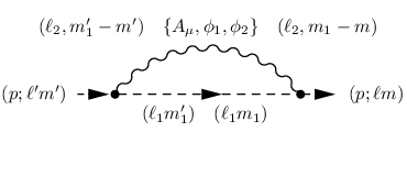
Figure 10: One loop diagram for correction to KK masses of Higgs bosons with virtual fermions.
Refer to caption
Figure 11: One loop diagram for correction to KK masses of Higgs bosons with virtual Higgs bosons.

The one loop diagrams corresponding to correction to KK masses of Higgs boson are given as Figs. 11-9 where corresponding quantum numbers {ℓ,m}\{\ell,m\} are shown for each external and internal lines. The Figs. 9 and 9 show the gauge boson loops including both four-dimensional components and extra-dimensional components from 4-point and 3-point gauge interactions. The Fig. 11 and 11 show the fermion and the Higgs boson loop contributions, respectively. Quantum correction to the KK masses of scalar boson can be organized in the same way as that of ϕi\phi_{i} such that

i​Ξ​(p2,μ,ℓ​m,ℓ​m′)=i​Ξbulk​(p2,ℓ​m,ℓ​m′)+i​Ξbound​(p2,μ,ℓ​m,ℓ​m′),\displaystyle i\Xi(p^{2};\mu;\ell m;\ell m^{\prime})=i\Xi_{\rm bulk}(p^{2};\ell m;\ell m^{\prime})+i\Xi_{\rm bound}(p^{2};\mu;\ell m;\ell m^{\prime}), (84)
i​Ξbulk⁡(bound)​(p2​(p2,μ),ℓ​m,ℓ​m′)=p2​i​Ξbulk⁡(bound)​(p2=0​(p2=0,μ),ℓ​m,ℓ​m′)\displaystyle i\Xi_{\rm bulk(bound)}(p^{2}(p^{2};\mu);\ell m;\ell m^{\prime})=p^{2}i\Xi_{\rm bulk(bound)}(p^{2}=0(p^{2}=0;\mu);\ell m;\ell m^{\prime})
−i​Ξ~bulk⁡(bound)​(p2=0​(p2=0,μ),ℓ​m,ℓ​m′),\displaystyle\hskip 170.71652pt-i\tilde{\Xi}_{\rm bulk(bound)}(p^{2}=0(p^{2}=0;\mu);\ell m;\ell m^{\prime}), (85)

where we list the contribution from each diagrams in Table 16 and 17. The RHS of Eq. (85) corresponds to the expansion in terms of p2p^{2} as in the previous case, and we omit p2=0p^{2}=0 in Ξ⁡(Ξ~)\Xi(\tilde{\Xi}) hereafter. Thus the correction to the Lagrangian is

δ​L1​l​o​o​p=\displaystyle\delta L_{\rm 1loop}= Ξbulk(i)​(ℓ​m,ℓ​m)​∂μHℓ​m†​∂μHℓ​m−Ξ~bulk(i)​(ℓ​m,ℓ​m)​Hℓ​m†​Hℓ​m\displaystyle\Xi_{\rm bulk}^{(i)}(\ell m;\ell m)\partial_{\mu}H_{\ell m}^{\dagger}\partial^{\mu}H_{\ell m}-\tilde{\Xi}_{\rm bulk}^{(i)}(\ell m;\ell m)H_{\ell m}^{\dagger}H_{\ell m}
+Ξbound(i)(μ;ℓm;ℓm)∂μHℓ​m†∂μHi​ℓ​m−Ξ~bound(i)(μ;ℓm;ℓm)Hℓ​m†Hℓ​m\displaystyle+\Xi_{\rm bound}^{(i)}(\mu;\ell m;\ell m)\partial_{\mu}H_{\ell m}^{\dagger}\partial^{\mu}H_{i\ell m}-\tilde{\Xi}_{\rm bound}^{(i)}(\mu;\ell m;\ell m)H_{\ell m}^{\dagger}H_{\ell m} (86)

where Ξ⁡(Ξ~)\Xi(\tilde{\Xi})s in the RHS are understood as the sum of corresponding contributions from all diagrams.

The renormalization condition and one-loop corrections to KK mass are also discussed as in the case of ϕi\phi_{i}. Repeating the same procedures as the case of ϕi\phi_{i}, we obtain counter terms

δH​∂μHℓ​m†​∂μHℓ​m−Mℓ2​δH​Hℓ​m†​Hℓ​m,\delta_{H}\partial_{\mu}H_{\ell m}^{\dagger}\partial^{\mu}H_{\ell m}-M_{\ell}^{2}\delta_{H}H_{\ell m}^{\dagger}H_{\ell m}, (87)

by the renormalization of field H→ZH​H=1+δHH\rightarrow\sqrt{Z_{H}}H=\sqrt{1+\delta_{H}}. We then apply the renormalization condition

(Ξbulk​(ℓ​m,ℓ​m)−δH)∣Mℓ​m​a​x2=Λ2=0,(\Xi_{\rm bulk}(\ell m;\ell m)-\delta_{H})\mid_{M_{\ell max}^{2}=\Lambda^{2}}=0, (88)

at a cut-off scale Λ\Lambda, requiring the canonical form of kinetic term at the cut-off scale. Then we carry out the normalization of fields

Hℓ​m→(1+Ξbulk​(ℓ​m,ℓ​m)+Ξbound​(μ,ℓ​m,ℓ​m)+δH)−12​Hℓ​m,H_{\ell m}\rightarrow\left(1+\Xi_{\rm bulk}(\ell m;\ell m)+\Xi_{\rm bound}(\mu;\ell m;\ell m)+\delta_{H}\right)^{-\frac{1}{2}}H_{\ell m}, (89)

same as above cases. Therefore we obtain the one-loop corrections to KK mass

M~ℓ​m2=\displaystyle\tilde{M}_{\ell m}^{2}= Mℓ2+Ξ~bulk​(ℓ​m,ℓ​m)+Ξ~bound​(μ,ℓ​m,ℓ​m)−Mℓ2​[Ξbulk​(ℓ​m,ℓ​m)+Ξbound​(μ,ℓ​m,ℓ​m)]\displaystyle M_{\ell}^{2}+\tilde{\Xi}_{\rm bulk}(\ell m;\ell m)+\tilde{\Xi}_{\rm bound}(\mu;\ell m;\ell m)-M_{\ell}^{2}\bigl[\Xi_{\rm bulk}(\ell m;\ell m)+\Xi_{\rm bound}(\mu;\ell m;\ell m)\bigr]
≡\displaystyle\equiv Mℓ2+(δ​M2)ℓ​mH,\displaystyle M_{\ell}^{2}+(\delta M^{2})^{H}_{\ell m}, (90)

for each KK mode of scalar boson, where we have taken the first order in Ξ\Xi and δ\delta in RHS.

IV KK mass spectrum and LKP

In this section, we estimate the one-loop corrections to KK masses for the first KK modes of SM fermions shown in Table 1, SM gauge bosons, and Higgs boson. In estimating these corrections, we take the renormalization scale μ\mu and the external momentum p2p^{2} to be the first KK mass μ2=2/R2\mu^{2}=2/R^{2} and p2=−2/R2p^{2}=-2/R^{2} respectively, and four-momentum cut-off scale Λ\Lambda as a parameter. Then angular momentum cut-off ℓm​a​x\ell_{max} is taken to be the maximum integer satisfying ℓm​a​x​(ℓm​a​x+1)/R≤Λ\sqrt{\ell_{max}(\ell_{max}+1)}/R\leq\Lambda. We specify the lightest KK particle which is expected to be the dark matter candidate.

To estimate the one-loop corrections to KK masses for SM fermions, we need to calculate coefficients Σ⁡(Σ~)\Sigma(\tilde{\Sigma})s in Eq. (58) from one-loop diagrams. For each fermions in Table 1, the coefficients Σ⁡(Σ~)\Sigma(\tilde{\Sigma})s obtain contributions from each diagrams such that

Σ⁡(Q)=ΣFig.2Q​Gμ+ΣFig.2Q​Wμ+ΣFig.2Q​Bμ+∑i=1,2[ΣFig.2Q​Gi+ΣFig.2Q​Wi+ΣFig.2Q​Bi]+ΣFig.2Q​H\displaystyle\Sigma(Q)=\Sigma^{QG_{\mu}}_{\rm Fig.\ref{Loop1}}+\Sigma^{QW_{\mu}}_{\rm Fig.\ref{Loop1}}+\Sigma^{QB_{\mu}}_{\rm Fig.\ref{Loop1}}+\sum_{i=1,2}\Bigl[\Sigma^{QG_{i}}_{\rm Fig.\ref{Loop1}}+\Sigma^{QW_{i}}_{\rm Fig.\ref{Loop1}}+\Sigma^{QB_{i}}_{\rm Fig.\ref{Loop1}}\Bigr]+\Sigma^{QH}_{\rm Fig.\ref{Loop2}} (91)
Σ⁡(U)=ΣFig.2U​Gμ+ΣFig.2U​Bμ+∑i=1,2[ΣFig.2U​Gi+ΣFig.2U​Bi]+ΣFig.2U​H\displaystyle\Sigma(U)=\Sigma^{UG_{\mu}}_{\rm Fig.\ref{Loop1}}+\Sigma^{UB_{\mu}}_{\rm Fig.\ref{Loop1}}+\sum_{i=1,2}\Bigl[\Sigma^{UG_{i}}_{\rm Fig.\ref{Loop1}}+\Sigma^{UB_{i}}_{\rm Fig.\ref{Loop1}}\Bigr]+\Sigma^{UH}_{\rm Fig.\ref{Loop2}} (92)
Σ⁡(D)=ΣFig.2D​Gμ+ΣFig.2D​Bμ+∑i=1,2[ΣFig.2D​Gi+ΣFig.2D​Bi]+ΣFig.2D​H\displaystyle\Sigma(D)=\Sigma^{DG_{\mu}}_{\rm Fig.\ref{Loop1}}+\Sigma^{DB_{\mu}}_{\rm Fig.\ref{Loop1}}+\sum_{i=1,2}\Bigl[\Sigma^{DG_{i}}_{\rm Fig.\ref{Loop1}}+\Sigma^{DB_{i}}_{\rm Fig.\ref{Loop1}}\Bigr]+\Sigma^{DH}_{\rm Fig.\ref{Loop2}} (93)
Σ⁡(L)=ΣFig.2L​Wμ+ΣFig.2L​Bμ+∑i=1,2[ΣFig.2L​Wi+ΣFig.2L​Bi]+ΣFig.2L​H\displaystyle\Sigma(L)=\Sigma^{LW_{\mu}}_{\rm Fig.\ref{Loop1}}+\Sigma^{LB_{\mu}}_{\rm Fig.\ref{Loop1}}+\sum_{i=1,2}\Bigl[\Sigma^{LW_{i}}_{\rm Fig.\ref{Loop1}}+\Sigma^{LB_{i}}_{\rm Fig.\ref{Loop1}}\Bigr]+\Sigma^{LH}_{\rm Fig.\ref{Loop2}} (94)
Σ⁡(E)=ΣFig.2E​Bμ+∑i=1,2[ΣFig.2E​Bi]+ΣFig.2E​H,\displaystyle\Sigma(E)=\Sigma^{EB_{\mu}}_{\rm Fig.\ref{Loop1}}+\sum_{i=1,2}\Bigl[\Sigma^{EB_{i}}_{\rm Fig.\ref{Loop1}}\Bigr]+\Sigma^{EH}_{\rm Fig.\ref{Loop2}}, (95)

where Σ~\tilde{\Sigma}s are given in the same way, and each terms in the RHS are the contributions from different loop diagrams with particles running in a loop shown as superscripts; the GμG_{\mu}, WμW_{\mu} and BμB_{\mu} denote the SU(3), SU(2) and U(1)Y gauge fields respectively, the GiG_{i}, WiW_{i} and BiB_{i} denote corresponding extra dimensional components ϕi\phi_{i}, and the H denotes the Higgs boson. Here we take into account contribution from Higgs-loop only for fermions in the 3rd generations since the Yukawa couplings for the 1st and the 2nd generations are small. The contributions to each coefficients are obtained from Table 9 applying corresponding gauge couplings g6​ag_{6a} and (Ta)2(T^{a})^{2} factor regarding the particles inside a loop; g6​a=1,2,3g_{6a=1,2,3} for U(1)Y, SU(2) and SU(3) gauge coupling, and (Ta)2={Y2,C2​(N),C2​(N)}(T^{a})^{2}=\{Y^{2},C_{2}(N),C_{2}(N)\} where C2​(N)=(N2−1)/2​NC_{2}(N)=(N^{2}-1)/2N for fundamental representation. We also note that each gauge couplings, Yukawa couplings and the Higgs self coupling in six-dimensions {g6​a,Yu,d,e,λ6}\{g_{6a},Y_{u,d,e},\lambda_{6}\} are related to that in four-dimensions as ga​(yu,e,d)=g6​a​(Yu,d,e)/4​π​R2g_{a}(y_{u,e,d})=g_{6a}(Y_{u,d,e})/\sqrt{4\pi R^{2}} and λ=λ6/(4​π​R2)\lambda=\lambda_{6}/(4\pi R^{2}) since the factor 4​π​R24\pi R^{2} comes from the surface area of S2S^{2} and 1/4​π1/\sqrt{4\pi} factor comes from mode functions for zero mode.

The mass matrix for fermion Eq. (16) is corrected by quantum correction as

Lmf=(ψ¯ℓ​mFψ¯ℓ​mf)T​(Mℓ+(δ​M)ℓ​mFmSM−12​mSM​δ​Nℓ​m;ΛmSM−12​mSM​δ​Nℓ​m;Λ−(Mℓ+(δ​M)ℓ​mf))​(ψℓ​mFψℓ​mf)\displaystyle L_{m_{f}}=\begin{pmatrix}\bar{\psi}_{\ell m}^{F}\\ \bar{\psi}_{\ell m}^{f}\end{pmatrix}^{T}\begin{pmatrix}M_{\ell}+(\delta M)_{\ell m}^{F}&m_{\rm SM}-\frac{1}{2}m_{\rm SM}\delta N_{\ell m;\Lambda}\\ m_{\rm SM}-\frac{1}{2}m_{\rm SM}\delta N_{\ell m;\Lambda}&-(M_{\ell}+(\delta M)_{\ell m}^{f})\end{pmatrix}\begin{pmatrix}\psi_{\ell m}^{F}\\ \psi_{\ell m}^{f}\end{pmatrix} (96)

where (δ​M)ℓ​mf⁡(F)(\delta M)^{f(F)}_{\ell m} is given by Eq. (65) and indices F⁡(f)F(f) show corresponding fermion comes from SU(2) doublet(singlet). Here we write one-loop correction to KK mass (δ​M)ℓ​mf⁡(F)(\delta M)^{f(F)}_{\ell m} as a product of 1/R1/R and dimensionless numerical factor Δℓ​m;Λf⁡(F)\Delta_{\ell m;\Lambda}^{f(F)} which depends on {ℓ,m}\{\ell,m\} and Λ\Lambda, such as

(δ​M)ℓ​mf⁡(F)=Δℓ​m;Λf⁡(F)​1R,(\delta M)^{f(F)}_{\ell m}=\Delta_{\ell m;\Lambda}^{f(F)}\frac{1}{R}, (97)

and we list the numerical factor Δℓ​m;Λf⁡(F)\Delta_{\ell m;\Lambda}^{f(F)} in Table 2 for the first KK mode. The correction to off-diagonal components are induced by normalization of field Eq. (64) such that

δ​Nℓ​m;Λ=(ΣbulkL+ΣboundL)F​(p2,μ,ℓ​m,ℓ​m)+δLF+(ΣbulkR+ΣboundR)f​(p2,μ,ℓ​m,ℓ​m)+δRf,\displaystyle\delta N_{\ell m;\Lambda}=(\Sigma^{L}_{\rm bulk}+\Sigma^{L}_{\rm bound})^{F}(p^{2};\mu;\ell m;\ell m)+\delta_{L}^{F}+(\Sigma^{R}_{\rm bulk}+\Sigma^{R}_{\rm bound})^{f}(p^{2};\mu;\ell m;\ell m)+\delta_{R}^{f}, (98)

where we have taken the first order of {Σ,δ}\{\Sigma,\delta\}, and the values of δ​Nℓ​m;Λ\delta N_{\ell m;\Lambda} is shown in Table 4 for the first KK mode. We thus obtain the KK mass eigenvalues

m~ℓ​mf1=\displaystyle\tilde{m}_{\ell m}^{f_{1}}= 12​[(δ​M)ℓ​mf−(δ​M)ℓ​mF+2​Mℓ2+mS​M2​[1+Mℓ​((δ​M)ℓ​mf+(δ​M)ℓ​mF)−mS​M​δ​Nℓ​m;ΛMℓ2+mS​M2]],\displaystyle\frac{1}{2}\Bigl[(\delta M)^{f}_{\ell m}-(\delta M)^{F}_{\ell m}+2\sqrt{M_{\ell}^{2}+m_{SM}^{2}}\Bigl[1+\frac{M_{\ell}((\delta M)^{f}_{\ell m}+(\delta M)^{F}_{\ell m})-m_{SM}\delta N_{\ell m;\Lambda}}{M_{\ell}^{2}+m_{SM}^{2}}\Bigr]\Bigr], (99)
m~ℓ​mf2=\displaystyle\tilde{m}_{\ell m}^{f_{2}}= −12​[(δ​M)ℓ​mf−(δ​M)ℓ​mF−2​Mℓ2+mS​M2​[1+Mℓ​((δ​M)ℓ​mf+(δ​M)ℓ​mF)−mS​M​δ​Nℓ​m;ΛMℓ2+mS​M2]],\displaystyle-\frac{1}{2}\Bigl[(\delta M)^{f}_{\ell m}-(\delta M)^{F}_{\ell m}-2\sqrt{M_{\ell}^{2}+m_{SM}^{2}}\Bigl[1+\frac{M_{\ell}((\delta M)^{f}_{\ell m}+(\delta M)^{F}_{\ell m})-m_{SM}\delta N_{\ell m;\Lambda}}{M_{\ell}^{2}+m_{SM}^{2}}\Bigr]\Bigr], (100)

for each KK modes of fermions, where we have taken the first order of {δ​M,δ​N}\{\delta M,\delta N\} in the RHS. The one-loop corrections to masses of the first KK modes for each fermion are shown in Table 5 and left-panel of Fig. 12.

ℓm​a​x\ell_{max} 22 33 44 55
Δ11,ΛER\Delta_{11,\Lambda}^{E_{R}} 0.00232 0.00726 0.00650 0.0167
Δ11,ΛLL\Delta_{11,\Lambda}^{L_{L}} 0.00635 0.0199 0.0178 0.0455
Δ11,ΛQL\Delta_{11,\Lambda}^{Q_{L}} 0.0418 0.110 0.126 0.242
Δ11,ΛUR\Delta_{11,\Lambda}^{U_{R}} 0.0370 0.116 0.104 0.265
Δ11,ΛDR\Delta_{11,\Lambda}^{D_{R}} 0.0362 0.113 0.101 0.259
Δ11,ΛbL\Delta_{11,\Lambda}^{b_{L}} 0.0418 0.133 0.116 0.304
Δ11,ΛbR\Delta_{11,\Lambda}^{b_{R}} 0.0345 0.113 0.100 0.261
Δ11,ΛtL\Delta_{11,\Lambda}^{t_{L}} 0.0434 0.136 0.120 0.310
Δ11,ΛtR\Delta_{11,\Lambda}^{t_{R}} 0.0362 0.118 0.103 0.272
Table 2: The numerical coefficients Δℓ​mf⁡(F)\Delta_{\ell m}^{f(F)} in Eq. (97) for ℓ=1,|m|=1\ell=1,|m|=1 as a function of ℓm​a​x\ell_{max}, where bL⁡(R)b_{L(R)} and tL⁡(R)t_{L(R)} are KK b quark and KK top quark from the SU(2) doublet(singlet).
ℓm​a​x\ell_{max} 22 33 44 55
Δ11,ΛBμ\Delta_{11,\Lambda}^{B_{\mu}} −0.0467-0.0467 −0.141-0.141 −0.637-0.637 −1.128-1.128
Δ11,ΛWμ\Delta_{11,\Lambda}^{W_{\mu}} 0.100 0.677 0.758 2.57
Δ11,ΛGμ\Delta_{11,\Lambda}^{G_{\mu}} 0.513 3.23 4.52 13.6
Δ11,ΛB1\Delta_{11,\Lambda}^{B_{1}} 0.1200.120 0.4530.453 1.361.36 2.862.86
Δ11,ΛW1\Delta_{11,\Lambda}^{W_{1}} 0.118 1.89 2.38 10.2
Δ11,ΛG1\Delta_{11,\Lambda}^{G_{1}} 0.283 8.98 8.65 46.6
Δ11,ΛH\Delta_{11,\Lambda}^{H} −0.0064-0.0064 −0.0167-0.0167 −0.0362-0.0362 −0.0269-0.0269
Table 3: The numerical coefficients Δℓ​mAμ,ϕ1\Delta_{\ell m}^{A_{\mu},\phi_{1}} in Eq. (105) and (115) for ℓ=1,|m|=1\ell=1,|m|=1 as a function of ℓm​a​x\ell_{max}.
ℓm​a​x\ell_{max} 22 33 44 55
δ​N11;Λτ\delta N_{11;\Lambda}^{\tau} 0.00237 0.00223 0.00400 0.00274
δ​N11;Λb\delta N_{11;\Lambda}^{b} 0.0229 0.0276 0.0397 0.0356
δ​N11;Λt\delta N_{11;\Lambda}^{t} 0.0244 0.0301 0.0432 0.0404
δ​N11;ΛBμ\delta N_{11;\Lambda}^{B_{\mu}} −0.0036-0.0036 −0.0098-0.0098 −0.0154-0.0154 −0.0250-0.0250
δ​N11;ΛWμ\delta N_{11;\Lambda}^{W_{\mu}} −0.0014-0.0014 −0.0067-0.0067 −0.0129-0.0129 −0.0240-0.0240
δ​N11;ΛB1\delta N_{11;\Lambda}^{B_{1}} −0.00267-0.00267 −0.000777-0.000777 −0.00622-0.00622 −0.000748-0.000748
δ​N11;ΛW1\delta N_{11;\Lambda}^{W_{1}} −0.00532-0.00532 −0.00152-0.00152 −0.0124-0.0124 −0.00149-0.00149
δ​N11;ΛH\delta N_{11;\Lambda}^{H} −0.00364-0.00364 −0.00662-0.00662 −0.0151-0.0151 −0.0232-0.0232
Table 4: The numerical coefficients δ​Nℓ​m;Λψ,A,ϕ1,H\delta N_{\ell m;\Lambda}^{\psi,A,\phi_{1},H} in Eq. (98), (106), (116) and (123) for ℓ=1,|m|=1\ell=1,|m|=1 as a function of ℓm​a​x\ell_{max}. Here the coefficients of only third generation of fermions are shown for fermion.

To estimate the one-loop corrections to KK masses for four-dimensional gauge bosons, we need to calculate coefficients Π\Pis in Eq. (68) from one-loop diagrams. For each gauge bosons, the coefficients Π⁡(Π~)\Pi(\tilde{\Pi})s obtain contributions from each diagrams such that

Π⁡(Gμ)=\displaystyle\Pi(G_{\mu})= ∑fΠFig.4f​f+ΠFig.4H​H+ΠFig.6H+ΠFig.6Gμ​Gμ+ΠFig.7Gμ\displaystyle\sum_{f}\Pi^{ff}_{\rm Fig.\ref{Loop3}}+\Pi^{HH}_{\rm Fig.\ref{Loop4}}+\Pi^{H}_{\rm Fig.\ref{Loop5}}+\Pi^{G_{\mu}G_{\mu}}_{\rm Fig.\ref{Loop6}}+\Pi^{G_{\mu}}_{\rm Fig.\ref{Loop7}}
+∑i=1,2ΠGμ​GiFig.6+∑i=1,2ΠGiFig.7+∑i,j=1,2ΠGi​GjFig.6+ΠcG​cGFig.4,\displaystyle+\sum_{i=1,2}\Pi^{G_{\mu}G_{i}}_{\rm Fig.\ref{Loop6}}+\sum_{i=1,2}\Pi^{G_{i}}_{\rm Fig.\ref{Loop7}}+\sum_{i,j=1,2}\Pi^{G_{i}G_{j}}_{\rm Fig.\ref{Loop6}}+\Pi^{c_{G}c_{G}}_{\rm Fig.\ref{Loop4}}, (101)
Π⁡(Wμ)=\displaystyle\Pi(W_{\mu})= ∑fΠFig.4f​f+ΠFig.4H​H+ΠFig.6H+ΠFig.6Wμ​Wμ+ΠFig.7Wμ\displaystyle\sum_{f}\Pi^{ff}_{\rm Fig.\ref{Loop3}}+\Pi^{HH}_{\rm Fig.\ref{Loop4}}+\Pi^{H}_{\rm Fig.\ref{Loop5}}+\Pi^{W_{\mu}W_{\mu}}_{\rm Fig.\ref{Loop6}}+\Pi^{W_{\mu}}_{\rm Fig.\ref{Loop7}}
+∑i=1,2ΠWμ​WiFig.6+∑i=1,2ΠWiFig.7+∑i,j=1,2ΠWi​WjFig.6+ΠcW​cWFig.4,\displaystyle+\sum_{i=1,2}\Pi^{W_{\mu}W_{i}}_{\rm Fig.\ref{Loop6}}+\sum_{i=1,2}\Pi^{W_{i}}_{\rm Fig.\ref{Loop7}}+\sum_{i,j=1,2}\Pi^{W_{i}W_{j}}_{\rm Fig.\ref{Loop6}}+\Pi^{c_{W}c_{W}}_{\rm Fig.\ref{Loop4}}, (102)
Π⁡(Bμ)=\displaystyle\Pi(B_{\mu})= ∑fΠFig.4f​f+ΠFig.4H​H+ΠFig.6H,\displaystyle\sum_{f}\Pi^{ff}_{\rm Fig.\ref{Loop3}}+\Pi^{HH}_{\rm Fig.\ref{Loop4}}+\Pi^{H}_{\rm Fig.\ref{Loop5}}, (103)

where Π~\tilde{\Pi}s are given in the same way, each terms in the RHS are the contributions from different loop diagrams with particles running in a loop shown as superscripts, and cG,Wc_{G,W} are ghost fields corresponding to GμG_{\mu} and WμW_{\mu} respectively. The contributions to each coefficients are obtained from Table 10 and 11. For a U(1)Y gauge field BμB_{\mu} and a SU(2) gauge field Wμ3W^{3}_{\mu}, the mass matrix at one-loop level is given as

(Bℓ​m​μWℓ​m​μ3)T​(Mℓ2+(δ​M2)ℓ​mB+14​g12​v2​(1+δ​NB)14​g1​g2​v2​(1+12​δ​NW+12​δ​NB)14​g1​g2​v2​(1+12​δ​NW+12​δ​NB)Mℓ2+(δ​M2)ℓ​mW+14​g12​v2​(1+δ​NW))​(Bℓ​mμWℓ​m3​μ)\begin{pmatrix}B_{\ell m\mu}\\ W^{3}_{\ell m\mu}\end{pmatrix}^{T}\begin{pmatrix}M_{\ell}^{2}+(\delta M^{2})_{\ell m}^{B}+\frac{1}{4}g_{1}^{2}v^{2}(1+\delta N^{B})&\frac{1}{4}g_{1}g_{2}v^{2}\Bigl(1+\frac{1}{2}\delta N^{W}+\frac{1}{2}\delta N^{B}\Bigr)\\ \frac{1}{4}g_{1}g_{2}v^{2}\Bigl(1+\frac{1}{2}\delta N^{W}+\frac{1}{2}\delta N^{B}\Bigr)&M_{\ell}^{2}+(\delta M^{2})_{\ell m}^{W}+\frac{1}{4}g_{1}^{2}v^{2}(1+\delta N^{W})\end{pmatrix}\begin{pmatrix}B^{\mu}_{\ell m}\\ W^{3\mu}_{\ell m}\end{pmatrix} (104)

where (δ​M2)ℓ​mB(\delta M^{2})_{\ell m}^{B} and (δ​M2)ℓ​mW(\delta M^{2})_{\ell m}^{W} are given by Eq. (74) with coefficients Π⁡(Π~)\Pi(\tilde{\Pi})s of Eqs. (102) and (103) for BμB_{\mu} and WμiW_{\mu}^{i} respectively. Here we write (δ​M2)ℓ​mAμ(\delta M^{2})^{A_{\mu}}_{\ell m} as a product of 1/R21/R^{2} and numerical factor as in the fermion case, where Aμ={Bμ,Wμ,Gμ}A_{\mu}=\{B_{\mu},W_{\mu},G_{\mu}\} , such as

(δ​M2)ℓ​mAμ=Δℓ​m;ΛAμ​1R2,(\delta M^{2})^{A_{\mu}}_{\ell m}=\Delta_{\ell m;\Lambda}^{A_{\mu}}\frac{1}{R^{2}}, (105)

and we list the numerical factors Δℓ​m;ΛAμ\Delta_{\ell m;\Lambda}^{A_{\mu}} in Table 2 for the first KK mode. The correction to non-diagonal elements is induced by renormalization of field Eq. (73) such that

δ​Nℓ​m;ΛWμ,Bμ=Πbulk​(W,B)​(p2,ℓ​m,ℓ​m)+Πbound​(W,B)​(p2,μ,ℓ​m,ℓ​m)−δ3​(W,B)\delta N^{W_{\mu},B_{\mu}}_{\ell m;\Lambda}=\Pi_{\rm bulk}(W,B)(p^{2};\ell m;\ell m)+\Pi_{\rm bound}(W,B)(p^{2};\mu;\ell m;\ell m)-\delta_{3}(W,B) (106)

where we have taken up to the first order in Π\Pis, and the values of δ​NW,B\delta N^{W,B} are shown in Table 4 for the first KK mode. Diagonalizing the mass matrix, we obtain the KK masses of KK-photon and KK-Z boson at one-loop level such that

m~γμℓ2≃\displaystyle\tilde{m}_{\gamma^{\ell}_{\mu}}^{2}\simeq Mℓ2+12​mZ2+12​[(δ​M2)ℓ​mB+(δ​M2)ℓ​mW−(mZ2−mW2)​δ​Nℓ​m;ΛBμ−mW2​δ​Nℓ​m;ΛWμ]\displaystyle M_{\ell}^{2}+\frac{1}{2}m_{Z}^{2}+\frac{1}{2}[(\delta M^{2})^{B}_{\ell m}+(\delta M^{2})^{W}_{\ell m}-(m_{Z}^{2}-m_{W}^{2})\delta N^{B^{\mu}}_{\ell m;\Lambda}-m_{W}^{2}\delta N^{W^{\mu}}_{\ell m;\Lambda}]
−12​((δ​M2)ℓ​mB−(δ​M2)ℓ​mW)2+mZ4,\displaystyle-\frac{1}{2}\sqrt{((\delta M^{2})^{B}_{\ell m}-(\delta M^{2})^{W}_{\ell m})^{2}+m_{Z}^{4}}, (107)
m~Zμℓ2≃\displaystyle\tilde{m}_{Z^{\ell}_{\mu}}^{2}\simeq Mℓ2+12​mZ2+12​[(δ​M2)ℓ​mB+(δ​M2)ℓ​mW−(mZ2−mW2)​δ​Nℓ​m;ΛBμ−mW2​δ​Nℓ​m;ΛWμ]\displaystyle M_{\ell}^{2}+\frac{1}{2}m_{Z}^{2}+\frac{1}{2}[(\delta M^{2})^{B}_{\ell m}+(\delta M^{2})^{W}_{\ell m}-(m_{Z}^{2}-m_{W}^{2})\delta N^{B^{\mu}}_{\ell m;\Lambda}-m_{W}^{2}\delta N^{W^{\mu}}_{\ell m;\Lambda}]
+12​((δ​M2)ℓ​mB−(δ​M2)ℓ​mW)2+mZ4,\displaystyle+\frac{1}{2}\sqrt{((\delta M^{2})^{B}_{\ell m}-(\delta M^{2})^{W}_{\ell m})^{2}+m_{Z}^{4}}, (108)

where we ignored terms proportional to δ​NGB,W\delta N_{G}^{B,W} in the square root in the second line of RHS for both equation due to the smallness of the factor. For KK modes of W±W^{\pm} bosons and Gluon, the one-loop corrections to KK masses are

(m~ℓWμ±)2=Mℓ2+mW2+(δ​M2)ℓ​mW+mW2​δ​Nℓ​m;ΛWμ,\displaystyle(\tilde{m}_{\ell}^{W^{\pm}_{\mu}})^{2}=M_{\ell}^{2}+m_{W}^{2}+(\delta M^{2})^{W}_{\ell m}+m_{W}^{2}\delta N^{W^{\mu}}_{\ell m;\Lambda}, (109)
(m~ℓG)2=Mℓ2+(δ​M2)ℓ​mG,\displaystyle(\tilde{m}_{\ell}^{G})^{2}=M_{\ell}^{2}+(\delta M^{2})^{G}_{\ell m}, (110)

where (δ​M2)ℓ​mG(\delta M^{2})^{G}_{\ell m} is given by Eq. (74) with coefficients Eq. (101). The corrected masses of the first KK modes for each gauge bosons are shown in the Table 5 and the right-panel of Fig. 12.

ℓm​a​x\ell_{max} 22 33 44 55
m~11​(ER)\tilde{m}_{11}(E_{R}) (GeV) 708.3 710.7 710.4 715.4
m~11​(LL)\tilde{m}_{11}(L_{L}) (GeV) 710.3 717.1 716.0 729.9
m~11​(τ1)\tilde{m}_{11}(\tau_{1}) (GeV) 708.3 710.7 710.4 715.4
m~11​(τ2)\tilde{m}_{11}(\tau_{2}) (GeV) 710.3 717.1 716.0 729.9
m~11​(dR)\tilde{m}_{11}(d_{R}) (GeV) 725.2 763.8.4 757.8 836.8
m~11​(uR)\tilde{m}_{11}(u_{R}) (GeV) 725.6 765.0 758.9 839.6
m~11​(QL)\tilde{m}_{11}(Q_{L}) (GeV) 728.0 762.1 770.1 827.9
m~11​(b1)\tilde{m}_{11}(b_{1}) (GeV) 724.4 763.6 756.9 837.7
m~11​(b2)\tilde{m}_{11}(b_{2}) (GeV) 728.0 773.9 765.2 859.3
m~11​(t1)\tilde{m}_{11}(t_{1}) (GeV) 745.2 785.0 777.4 860.1
m~11​(t2)\tilde{m}_{11}(t_{2}) (GeV) 748.9 794.0 786.1 879.2
m~11​(γ)\tilde{m}_{11}(\gamma) (GeV) 701.4 684.7 587.2 428.4
m~11​(Z)\tilde{m}_{11}(Z) (GeV) 727.7 820.7 833.0 1071.
m~11​(W)\tilde{m}_{11}(W) (GeV) 729.0 822.1 834.2 1072.
m~11​(G)\tilde{m}_{11}(G) (GeV) 792.8 1144. 1276. 1973.
m~11​(γ1)\tilde{m}_{11}(\gamma_{1}) (GeV) 727.9 785.7 919.0 1105.
m~11​(Z1)\tilde{m}_{11}(Z_{1}) (GeV) 733.6 988.9 1049. 1746.
m~11​(W1)\tilde{m}_{11}(W_{1}) (GeV) 732.3 990.0 1050. 1746.
m~11​(G1)\tilde{m}_{11}(G_{1}) (GeV) 755.4 1656. 1632. 3485.
m~11​(H)\tilde{m}_{11}(H) (GeV) 717.1 715.3 711.7 713.3
Table 5: The one-loop correction the masses of the first KK modes (ℓ=1,|m|=1\ell=1,|m|=1) for each cut off scale where ℓm​a​x=2,3,4,5\ell_{max}=2,3,4,5 are taken as reference values. Here we have taken the inverse of S2/Z2S^{2}/Z_{2} radius as 1/R=5001/R=500 GeV, where the tree-level first KK mass corresponds to 2/R≃707\sqrt{2}/R\simeq 707 GeV.

To estimate the one-loop corrections to KK masses for physical extra-dimensional components of gauge fields ϕ1\phi_{1}, we need to calculate coefficients Θ⁡(Θ~)\Theta(\tilde{\Theta})s in Eq. (77) from one-loop diagrams. For each gauge bosons, the coefficients Θ⁡(Θ~)\Theta(\tilde{\Theta})s obtain contributions from each diagrams such that

Θ⁡(G1)=\displaystyle\Theta(G_{1})= ∑fΘFig.4(1)​f​f+ΘFig.4(1)​H​H+ΘFig.6(1)​H+ΘFig.6(1)​Gμ​Gμ+ΘFig.7(1)​Gμ\displaystyle\sum_{f}\Theta^{(1)ff}_{\rm Fig.\ref{Loop3}}+\Theta^{(1)HH}_{\rm Fig.\ref{Loop4}}+\Theta^{(1)H}_{\rm Fig.\ref{Loop5}}+\Theta^{(1)G_{\mu}G_{\mu}}_{\rm Fig.\ref{Loop6}}+\Theta^{(1)G_{\mu}}_{\rm Fig.\ref{Loop7}}
+∑a=1,2Θ(1)​Gμ​GaFig.6+∑a=1,2Θ(1)​GaFig.7+∑a,b=1,2Θ(1)​Ga​GbFig.6+Θ(1)​cG​cGFig.4,\displaystyle+\sum_{a=1,2}\Theta^{(1)G_{\mu}G_{a}}_{\rm Fig.\ref{Loop6}}+\sum_{a=1,2}\Theta^{(1)G_{a}}_{\rm Fig.\ref{Loop7}}+\sum_{a,b=1,2}\Theta^{(1)G_{a}G_{b}}_{\rm Fig.\ref{Loop6}}+\Theta^{(1)c_{G}c_{G}}_{\rm Fig.\ref{Loop4}}, (111)
Θ⁡(W1)=\displaystyle\Theta(W_{1})= ∑fΘFig.4(1)​f​f+ΘFig.4(1)​H​H+ΘFig.6(1)​H+ΘFig.6(1)​Wμ​Wμ+ΘFig.7(1)​Wμ\displaystyle\sum_{f}\Theta^{(1)ff}_{\rm Fig.\ref{Loop3}}+\Theta^{(1)HH}_{\rm Fig.\ref{Loop4}}+\Theta^{(1)H}_{\rm Fig.\ref{Loop5}}+\Theta^{(1)W_{\mu}W_{\mu}}_{\rm Fig.\ref{Loop6}}+\Theta^{(1)W_{\mu}}_{\rm Fig.\ref{Loop7}}
+∑a=1,2Θ(1)​Wμ​WaFig.6+∑a=1,2Θ(1)​WaFig.7+∑a,b=1,2Θ(1)​Wa​WbFig.6+Θ(1)​cW​cWFig.4,\displaystyle+\sum_{a=1,2}\Theta^{(1)W_{\mu}W_{a}}_{\rm Fig.\ref{Loop6}}+\sum_{a=1,2}\Theta^{(1)W_{a}}_{\rm Fig.\ref{Loop7}}+\sum_{a,b=1,2}\Theta^{(1)W_{a}W_{b}}_{\rm Fig.\ref{Loop6}}+\Theta^{(1)c_{W}c_{W}}_{\rm Fig.\ref{Loop4}}, (112)
Θ⁡(B1)=\displaystyle\Theta(B_{1})= ∑fΘFig.4(1)​f​f+ΘFig.4(1)​H​H+ΘFig.6(1)​H,\displaystyle\sum_{f}\Theta^{(1)ff}_{\rm Fig.\ref{Loop3}}+\Theta^{(1)HH}_{\rm Fig.\ref{Loop4}}+\Theta^{(1)H}_{\rm Fig.\ref{Loop5}}, (113)

where Θ~\tilde{\Theta}s are given in the same way, and each terms in the RHS are the contributions from different loop diagrams with particles running in a loop shown as superscripts. The contributions to each coefficients are obtained from Table 12 and 13. The one-loop corrections to KK masses for ϕ1\phi_{1} are similarly obtained as four dimensional case. For B1B_{1} and W13W^{3}_{1}, the corrected mass matrix is given as

(B1​ℓ​mW1​ℓ​m3)T​(Mℓ2+(δ​M2)ℓ​mB1+14​g12​v2​(1+δ​Nℓ​m;ΛB1)14​g1​g2​v2​(1+12​δ​Nℓ​m;ΛW1+12​δ​Nℓ​m;ΛB1)14​g1​g2​v2​(1+12​δ​Nℓ​m;ΛW1+12​δ​Nℓ​m;ΛB1)Mℓ2+(δ​M2)ℓ​mW1+14​g12​v2​(1+δ​Nℓ​m;ΛW1))​(B1​ℓ​mW1​ℓ​m3)\begin{pmatrix}B_{1\ell m}\\ W^{3}_{1\ell m}\end{pmatrix}^{T}\begin{pmatrix}M_{\ell}^{2}+(\delta M^{2})_{\ell m}^{B_{1}}+\frac{1}{4}g_{1}^{2}v^{2}(1+\delta N^{B_{1}}_{\ell m;\Lambda})&\frac{1}{4}g_{1}g_{2}v^{2}\Bigl(1+\frac{1}{2}\delta N^{W_{1}}_{\ell m;\Lambda}+\frac{1}{2}\delta N^{B_{1}}_{\ell m;\Lambda}\Bigr)\\ \frac{1}{4}g_{1}g_{2}v^{2}\Bigl(1+\frac{1}{2}\delta N^{W_{1}}_{\ell m;\Lambda}+\frac{1}{2}\delta N^{B_{1}}_{\ell m;\Lambda}\Bigr)&M_{\ell}^{2}+(\delta M^{2})_{\ell m}^{W_{1}}+\frac{1}{4}g_{1}^{2}v^{2}(1+\delta N^{W_{1}}_{\ell m;\Lambda})\end{pmatrix}\begin{pmatrix}B_{1\ell m}\\ W^{3}_{1\ell m}\end{pmatrix} (114)

where M~B1​ℓ​m2\tilde{M}_{B_{1\ell m}}^{2} and M~W1​ℓ​m2\tilde{M}_{W_{1\ell m}}^{2} are given by Eq. (83) with coefficients in Eqs. (112) and (113) for BiB_{i} and WiW_{i} respectively. Here we write (δ​M2)ℓ​mϕ1(\delta M^{2})^{\phi_{1}}_{\ell m} in the same form as Eq. (105), where ϕ1={B1,W1,G1}\phi_{1}=\{B_{1},W_{1},G_{1}\}, as

(δ​M2)ℓ​mϕ1=Δℓ​mϕ1​1R2,(\delta M^{2})^{\phi_{1}}_{\ell m}=\Delta_{\ell m}^{\phi_{1}}\frac{1}{R^{2}}, (115)

and we list the numerical factor Δℓ​mϕ1\Delta_{\ell m}^{\phi_{1}} in Table 2 for the first KK mode. The correction to off-diagonal elements is induced by the renormalization of field Eq. (82) such that

δ​Nℓ​m;ΛW1,B1=−Θbulk​(W,B)​(ℓ​m,ℓ​m)−Θbound​(W,B)​(μ,ℓ​m,ℓ​m)−δ3(1)​(W,B)\delta N_{\ell m;\Lambda}^{W_{1},B_{1}}=-\Theta_{\rm bulk}(W,B)(\ell m;\ell m)-\Theta_{\rm bound}(W,B)(\mu;\ell m;\ell m)-\delta_{3}^{(1)}(W,B) (116)

where we have taken up to the first order of Θ⁡(Θ~)\Theta(\tilde{\Theta}), and the values of δ​Nℓ​m;ΛW1,B1\delta N^{W_{1},B_{1}}_{\ell m;\Lambda} are shown in Table 4 for the first KK mode. Diagonalizing the mass matrix, we obtain the one-loop corrections to KK masses of extra dimensional components KK-photon and KK-Z boson such that

m~γ1ℓ2≃\displaystyle\tilde{m}_{\gamma^{\ell}_{1}}^{2}\simeq Mℓ2+12​mZ2+12​[(δ​M2)ℓ​mB1+(δ​M2)ℓ​mW1−(mZ2−mW2)​δ​Nℓ​m;ΛB1−mW2​δ​Nℓ​m;ΛW1]\displaystyle M_{\ell}^{2}+\frac{1}{2}m_{Z}^{2}+\frac{1}{2}[(\delta M^{2})^{B_{1}}_{\ell m}+(\delta M^{2})^{W_{1}}_{\ell m}-(m_{Z}^{2}-m_{W}^{2})\delta N^{B_{1}}_{\ell m;\Lambda}-m_{W}^{2}\delta N^{W_{1}}_{\ell m;\Lambda}]
−12​((δ​M2)ℓ​mB1−(δ​M2)ℓ​mW)2+mZ4,\displaystyle-\frac{1}{2}\sqrt{((\delta M^{2})^{B_{1}}_{\ell m}-(\delta M^{2})^{W}_{\ell m})^{2}+m_{Z}^{4}}, (117)
m~Z1ℓ2≃\displaystyle\tilde{m}_{Z^{\ell}_{1}}^{2}\simeq Mℓ2+12​mZ2+12​[(δ​M2)ℓ​mB1+(δ​M2)ℓ​mW1−(mZ2−mW2)​δ​Nℓ​m;ΛB1−mW2​δ​Nℓ​m;ΛW1]\displaystyle M_{\ell}^{2}+\frac{1}{2}m_{Z}^{2}+\frac{1}{2}[(\delta M^{2})^{B_{1}}_{\ell m}+(\delta M^{2})^{W_{1}}_{\ell m}-(m_{Z}^{2}-m_{W}^{2})\delta N^{B_{1}}_{\ell m;\Lambda}-m_{W}^{2}\delta N^{W_{1}}_{\ell m;\Lambda}]
+12​((δ​M2)ℓ​mB1−(δ​M2)ℓ​mW1)2+mZ4,\displaystyle+\frac{1}{2}\sqrt{((\delta M^{2})^{B_{1}}_{\ell m}-(\delta M^{2})^{W_{1}}_{\ell m})^{2}+m_{Z}^{4}}, (118)

where we ignored the terms proportional to δ​NϕB,W\delta N^{B,W}_{\phi} in square root in the second line of RHS for both equation due to the smallness of the factor. For KK modes of W±W^{\pm} bosons and Gluon, the one-loop corrections to KK masses are

(m~ℓW1±)2=Mℓ2+mW2+(δ​M2)ℓ​mW1+mW2​δ​Nℓ​m;ΛW1,\displaystyle(\tilde{m}_{\ell}^{W^{\pm}_{1}})^{2}=M_{\ell}^{2}+m_{W}^{2}+(\delta M^{2})^{W_{1}}_{\ell m}+m_{W}^{2}\delta N^{W_{1}}_{\ell m;\Lambda}, (119)
(m~ℓG1)2=Mℓ2+(δ​M2)ℓ​mG1,\displaystyle(\tilde{m}_{\ell}^{G_{1}})^{2}=M_{\ell}^{2}+(\delta M^{2})^{G_{1}}_{\ell m}, (120)

where (δ​M2)ℓ​mG1(\delta M^{2})^{G_{1}}_{\ell m} is given by Eq. (83) with coefficients in Eq. (111). The one-loop corrections to masses of the first KK modes for each ϕ1\phi_{1} are shown in Table 5 and the right-panel of Fig. 12.

Refer to caption
Refer to caption
Figure 12: The KK masses for the first KK modes at one-loop level. The left panel shows the KK masses for fermions and the right panel shows that of gauge bosons as the function of Λ​R\Lambda R. The angular momentum cut-off ℓm​a​x\ell_{max} is taken as the maximum integer satisfying ℓm​a​x​(ℓm​a​x+1)/R≤Λ\sqrt{\ell_{max}(\ell_{max}+1)}/R\leq\Lambda.

To estimate the one-loop corrections to KK masses for SM Higgs boson, we need to calculate coefficients Ξ⁡(Ξ~)\Xi(\tilde{\Xi}) in Eq. (86) from one-loop diagrams. The coefficients Ξ⁡(Ξ~)\Xi(\tilde{\Xi}) obtain contributions from each diagrams such that

Ξ⁡(H)=\displaystyle\Xi(H)= ∑fΞFig.11f​f+ΞFig.11H+ΞFig.9Wμ​H+ΞFig.9Bμ​H+ΞFig.9Wμ+ΞFig.9Bμ\displaystyle\sum_{f}\Xi^{ff}_{\rm Fig.\ref{Loop9}}+\Xi^{H}_{\rm Fig.\ref{Loop8}}+\Xi^{W_{\mu}H}_{\rm Fig.\ref{Loop11}}+\Xi^{B_{\mu}H}_{\rm Fig.\ref{Loop11}}+\Xi^{W_{\mu}}_{\rm Fig.\ref{Loop10}}+\Xi^{B_{\mu}}_{\rm Fig.\ref{Loop10}}
+∑iΞWiFig.9+∑iΞBiFig.9+∑iΞWi​HFig.9+∑iΞBi​HFig.9\displaystyle+\sum_{i}\Xi^{W_{i}}_{\rm Fig.\ref{Loop10}}+\sum_{i}\Xi^{B_{i}}_{\rm Fig.\ref{Loop10}}+\sum_{i}\Xi^{W_{i}H}_{\rm Fig.\ref{Loop11}}+\sum_{i}\Xi^{B_{i}H}_{\rm Fig.\ref{Loop11}} (121)

where Ξ~\tilde{\Xi} is given in the same way, and each terms in the RHS are the contributions from different loop diagrams with particles propagating inside a loop shown as superscripts. The one-loop corrections to KK masses for the KK Higgs boson are also obtained in a similar way such as

(m~ℓH)2=Mℓ2+mh2+(δ​M2)ℓ​mH+mh2​δ​Nℓ​m;ΛH(\tilde{m}_{\ell}^{H})^{2}=M_{\ell}^{2}+m_{h}^{2}+(\delta M^{2})^{H}_{\ell m}+m_{h}^{2}\delta N^{H}_{\ell m;\Lambda} (122)

where the fourth term in RHS is induced by normalization of field Eq. (89) such that

δ​Nℓ​m;ΛH=−Ξbulk​(ℓ​m,ℓ​m)−Ξbound​(μ,ℓ​m,ℓ​m)−δ3H\delta N^{H}_{\ell m;\Lambda}=-\Xi_{\rm bulk}(\ell m;\ell m)-\Xi_{\rm bound}(\mu;\ell m;\ell m)-\delta_{3}^{H} (123)

taking up to the first order of Ξ\Xis, and the values of δ​NH\delta N^{H} are shown in Table 4. The (δ​M2)ℓ​mH(\delta M^{2})^{H}_{\ell m} is also written as Eq. (105) such that

(δ​M2)ℓ​mH=Δℓ​m;ΛH​1R2,(\delta M^{2})^{H}_{\ell m}=\Delta_{\ell m;\Lambda}^{H}\frac{1}{R^{2}}, (124)

and we list the numerical factor Δℓ​m;ΛH\Delta_{\ell m;\Lambda}^{H} in Table 2. Also the one-loop corrections to masses of the first KK modes for Higgs bosons are shown in Table 5 and the right-panel of Fig. 12.

The Table 5 shows the one-loop corrections to KK mass of the first KK modes ℓ=1,|m|=1\ell=1,|m|=1 for each SM particles where we take cut off ℓm​a​x=2,3,4,5\ell_{max}=2,3,4,5 as reference values. From the Table we can see that the first KK photon has the lightest KK mass for any cut-off scale. The first KK photon thus is a promising candidate of the dark matter in the model. The smallest correction to the KK photon mass is due to the negative contributions from fermion loops while the non-Abelian gauge bosons obtain large contribution from the loops associated with self-interactions. We also find that negative contribution from fermion loops to KK masses of ϕ1\phi_{1} tends to be less effective compared with the case of four-dimensional components, and the one-loop corrections to the KK masses become larger than that of four-dimensional components. We show the cut-off scale dependence of the first KK masses in the Fig. 12, where we ignored the SM masses of e,μ,u,d,s,ce,\mu,u,d,s,c and write as ER,L,uR,dR,QLE_{R},L,u_{R},d_{R},Q_{L} for SU(2) singlet charged lepton, doublet lepton, singlet quarks and doublet quarks respectively. We also note that zig-zag shaped lines appear in Fig. 12 where the discontinuity of the plot corresponds to increase of ℓm​a​x\ell_{max} at Λ​R=ℓm​a​x​(ℓm​a​x+1)\Lambda R=\sqrt{\ell_{max}(\ell_{max}+1)} and the corrected masses tend to be small for even ℓmax\ell_{\rm max} compared to odd one. This tendency is due to the sign factor of (−1){ℓ,m}(-1)^{\{\ell,m\}} which appears from propagator and vertices on S2/Z2S^{2}/Z_{2} and gives different sign contribution from each KK modes in the loops as mentioned below Eq. (57). Since number of negative and positive sign contributions is different for even or odd ℓmax\ell_{\rm max} case, the corrected mass depend on ℓmax\ell_{\rm max} differently for even or odd case. The quantum corrections tend to be large for the large cut-off scale since the six dimensional loop expansion parameter ϵ=ga232​π2​(R​Λ)2\epsilon=\frac{g_{a}^{2}}{32\pi^{2}}(R\Lambda)^{2} becomes large. This indicates that the perturbation is not reliable and we cannot take a large cut-off scale, which is a generic feature of non-renormalizable theories.

V Summary and discussions

We have investigated the quantum correction of Kaluza-Klein masses in the S2/Z2S^{2}/Z_{2} universal extra dimensional model in order to determine the lightest KK particle which would be the dark matter candidate.

We first derived the Feynman rules for propagators and vertices on the six dimensional spacetime M4×S2/Z2M^{4}\times S^{2}/Z^{2}. We then calculated the one-loop diagrams relevant to one-loop corrections to the KK masses with the Feynman rules. The contributions from the one-loop diagrams can be separated to the bulk contribution conserving KK number mm and the boundary contribution violating the KK number conservation, which is the similar structure as in the minimal UED case. In calculating these diagrams, we introduced the cut-off for both 4-momentum integration and angular momentum sum inside a loop by defining the 4-momentum cut-off scale Λ\Lambda and the angular momentum number cut-off ℓm​a​x\ell_{max}. Thus the bulk contribution is estimated with cut-off scale Λ\Lambda as an upper bound of momentum integration while the boundary contribution is estimated by taking leading log-divergent part assuming vanishing contribution at the cut-off scale. The contributions from the one loop diagrams are then organized as the form of Eq. (58), (68), (77) and (86) for fermions, gauge bosons, extra dimensional components gauge bosons and scalar bosons respectively, and the explicit form of the contributions are summarized in the Table 9, 10, 11, 12, 13, 15, 16 and 17. Taking into account the renormalization conditions, we finally obtained the formula to derive the corrected KK masses as Eq. (65), (74), (83) and (90) for fermions, gauge bosons, extra dimensional components gauge bosons and scalar bosons respectively.

At last we estimated the corrected KK masses of first KK mode (ℓ=1,|m|=1\ell=1,|m|=1) for each SM particles applying the formulas in Section III. The resulting corrected masses, taking 1/R=5001/R=500GeV as a reference value, are summarized in Table 5 for each cut-off. We then find that the lightest KK particle is the 1st KK photon γμ11\gamma^{11}_{\mu} as in the minimal UED case, and it can be identified as the promising DM candidate. We have also shown the numerical plot of the one-loop correction to the first KK modes as a function of cut-off scale Λ\Lambda in the Fig. 12. We have found that the corrected masses tend to be small for even ℓm​a​x\ell_{max} compared to odd one due to the sign factor (−1){ℓ,m}(-1)^{\{\ell,m\}} which appears in loop diagram calculation. The quantum correction tend to be large for higher cut-off since the number of modes inside a loop becomes very large, which indicates that we can not take cut-off scale too large.

It would be very interesting to study the relic density of the dark matter candidate, γμ11\gamma^{11}_{\mu}, with the corrected mass spectrum, which will give constraints for the S2/Z2S^{2}/Z_{2} radius RR and the cut-off scale Λ\Lambda. Furthermore the one-loop corrections to the mass spectrum would lead a prediction of the experimental signature of our model and the analysis is left for future work.

Acknowledgements.
The work of N.M. was supported in part by the Grant-in-Aid for the Ministry of Education, Culture, Sports, Science, and Technology, Government of Japan (No. 24540283). The work of T.N. was supported in part by NSC Grant No. 102-2811-M-006-035. The work of J.S. was supported in part by the Grant-in-Aid for the Ministry of Education, Culture, Sports, Science, and Technology, Government of Japan (Nos. 24340044 and 25105009).

Appendix A Summary lists of vertices in our model

Here we summarize the Feynman rules for vertices in our model. The vertices including fermions are derived from gauge interactions and Yukawa interactions

∫d​x4​𝑑Ω​g6​a​Ψ¯±​ΓM​Tia​AMi​Ψ±,\displaystyle\int dx^{4}d\Omega g_{6a}\bar{\Psi}_{\pm}\Gamma^{M}T^{a}_{i}A_{M}^{i}\Psi_{\pm}, (125)
∫d​x4​𝑑Ω​Yf​Ψ¯±​H​Ψ∓\displaystyle\int dx^{4}d\Omega Y_{f}\bar{\Psi}_{\pm}H\Psi_{\mp} (126)

where Aθ,ϕA_{\theta,\phi} in Eqs. (20) and (21) are substituted. The Feynman rules for these vertices are listed in Table 6 where the non-trivial factors in these vertices are given by integrations of mode function as Eq. (46) for Iα⁡(β)I^{\alpha(\beta)}, and

Cℓ1​m1;ℓ2​m2;ℓ3​m3α=∫dΩα~ℓ1​m1∗(∂θ−isin⁡θ∂ϕ)Y~ℓ2​m2β~ℓ3​m3,\displaystyle C^{\alpha}_{\ell_{1}m_{1};\ell_{2}m_{2};\ell_{3}m_{3}}=\int d\Omega\tilde{\alpha}^{*}_{\ell_{1}m_{1}}\left(\partial_{\theta}-\frac{i}{\sin\theta}\partial_{\phi}\right)\tilde{Y}_{\ell_{2}m_{2}}\tilde{\beta}_{\ell_{3}m_{3}}, (127)
Cℓ1​m1;ℓ2​m2;ℓ3​m3β=−∫dΩβ~ℓ1​m1∗(∂θ+isin⁡θ∂ϕ)Y~ℓ2​m2α~ℓ3​m3.\displaystyle C^{\beta}_{\ell_{1}m_{1};\ell_{2}m_{2};\ell_{3}m_{3}}=-\int d\Omega\tilde{\beta}^{*}_{\ell_{1}m_{1}}\left(\partial_{\theta}+\frac{i}{\sin\theta}\partial_{\phi}\right)\tilde{Y}_{\ell_{2}m_{2}}\tilde{\alpha}_{\ell_{3}m_{3}}. (128)
Interaction vertex factor
Ψ±ℓ1​m1​Aμ​ℓ2​m2​Ψ±ℓ3​m3\Psi_{\pm\ell_{1}m_{1}}A_{\mu\ell_{2}m_{2}}\Psi_{\pm\ell_{3}m_{3}} i​g6​aR​Ta​γμ​[Iℓ1​m1;ℓ2​m2;ℓ3​m3α​PR⁡(L)+Iℓ1​m1;ℓ2​m2;ℓ3​m3β​PL⁡(R)]i\frac{g_{6a}}{R}T^{a}\gamma^{\mu}\left[I^{\alpha}_{\ell_{1}m_{1};\ell_{2}m_{2};\ell_{3}m_{3}}P_{R(L)}+I^{\beta}_{\ell_{1}m_{1};\ell_{2}m_{2};\ell_{3}m_{3}}P_{L(R)}\right]
Ψ±ℓ1​m1​ϕ1​ℓ2​m2​Ψ±ℓ3​m3\Psi_{\pm\ell_{1}m_{1}}\phi_{1\ell_{2}m_{2}}\Psi_{\pm\ell_{3}m_{3}} i​g6​aR​Ta​γ5​[Cℓ1​m1;ℓ2​m2;ℓ3​m3α​PL⁡(R)+Cℓ1​m1;ℓ2​m2;ℓ3​m3β​PR⁡(L)]i\frac{g_{6a}}{R}T^{a}\gamma_{5}\left[C^{\alpha}_{\ell_{1}m_{1};\ell_{2}m_{2};\ell_{3}m_{3}}P_{L(R)}+C^{\beta}_{\ell_{1}m_{1};\ell_{2}m_{2};\ell_{3}m_{3}}P_{R(L)}\right]
Ψ±ℓ1​m1​ϕ2​ℓ2​m2​Ψ±ℓ3​m3\Psi_{\pm\ell_{1}m_{1}}\phi_{2\ell_{2}m_{2}}\Psi_{\pm\ell_{3}m_{3}} i​g6​aR​Ta​γ5​[i​Cℓ1​m1;ℓ2​m2;ℓ3​m3α​PL⁡(R)−i​Cℓ1​m1;ℓ2​m2;ℓ3​m3β​PR⁡(L)]i\frac{g_{6a}}{R}T^{a}\gamma_{5}\left[iC^{\alpha}_{\ell_{1}m_{1};\ell_{2}m_{2};\ell_{3}m_{3}}P_{L(R)}-iC^{\beta}_{\ell_{1}m_{1};\ell_{2}m_{2};\ell_{3}m_{3}}P_{R(L)}\right]
Ψ∓ℓ1​m1​Hℓ2​m2​Ψ±ℓ3​m3\Psi_{\mp\ell_{1}m_{1}}H_{\ell_{2}m_{2}}\Psi_{\pm\ell_{3}m_{3}} i​YfR​[Iℓ1​m1;ℓ2​m2;ℓ3​m3α​PR⁡(L)+Iℓ1​m1;ℓ2​m2;ℓ3​m3β​PL⁡(R)]i\frac{Y_{f}}{R}\left[I^{\alpha}_{\ell_{1}m_{1};\ell_{2}m_{2};\ell_{3}m_{3}}P_{R(L)}+I^{\beta}_{\ell_{1}m_{1};\ell_{2}m_{2};\ell_{3}m_{3}}P_{L(R)}\right]
Table 6: The vertex factors for interactions including fermions where Yf=Yu,d,eY_{f}=Y_{u,d,e}.
Interaction vertex factor
Hℓ1​m1†​(p1)​Aμ​ℓ2​m2​Hℓ3​m3​(p2)H_{\ell_{1}m_{1}}^{\dagger}(p_{1})A_{\mu\ell_{2}m_{2}}H_{\ell_{3}m_{3}}(p_{2}) i​g6​aR​Ta​(p1μ+p2μ)​Jℓ1​m1¯;ℓ2​m2;ℓ3​m31i\frac{g_{6a}}{R}T^{a}(p_{1}^{\mu}+p_{2}^{\mu})J^{1}_{\underline{\ell_{1}m_{1}};\ell_{2}m_{2};\ell_{3}m_{3}}
Hℓ1​m1†​(p1)​ϕ1​ℓ2​m2​Hℓ3​m3​(p2)H_{\ell_{1}m_{1}}^{\dagger}(p_{1})\phi_{1\ell_{2}m_{2}}H_{\ell_{3}m_{3}}(p_{2}) −g6​aR​Ta​[Jℓ1​m1¯;ℓ2​m2;ℓ3​m32−Jℓ3​m3;ℓ2​m2;ℓ1​m1¯2]-\frac{g_{6a}}{R}T^{a}\big[J^{2}_{\underline{\ell_{1}m_{1}};\ell_{2}m_{2};\ell_{3}m_{3}}-J^{2}_{\ell_{3}m_{3};\ell_{2}m_{2};\underline{\ell_{1}m_{1}}}\big]
Hℓ1​m1†​(p1)​ϕ2​ℓ2​m2​Hℓ3​m3​(p2)H_{\ell_{1}m_{1}}^{\dagger}(p_{1})\phi_{2\ell_{2}m_{2}}H_{\ell_{3}m_{3}}(p_{2}) −g6​aR​Ta​[Jℓ1​m1¯;ℓ2​m2;ℓ3​m33−Jℓ3​m3;ℓ2​m2;ℓ1​m1¯3]-\frac{g_{6a}}{R}T^{a}\big[J^{3}_{\underline{\ell_{1}m_{1}};\ell_{2}m_{2};\ell_{3}m_{3}}-J^{3}_{\ell_{3}m_{3};\ell_{2}m_{2};\underline{\ell_{1}m_{1}}}\big]
Aℓ1​m1μ​Aℓ2​m2ν​Hℓ3​m3†​Hℓ4​m4A_{\ell_{1}m_{1}}^{\mu}A_{\ell_{2}m_{2}}^{\nu}H^{\dagger}_{\ell_{3}m_{3}}H_{\ell_{4}m_{4}} 2​i​g6​a2R2​Tia​Tja​gμ​ν​Kℓ1​m1;ℓ2​m2;ℓ3​m3¯;ℓ4​m412i\frac{g_{6a}^{2}}{R^{2}}T^{a}_{i}T^{a}_{j}g_{\mu\nu}K^{1}_{\ell_{1}m_{1};\ell_{2}m_{2};\underline{\ell_{3}m_{3}};\ell_{4}m_{4}}
ϕ1​(2)​ℓ1​m1​ϕ1​(2)​ℓ2​m2​Hℓ3​m3†​Hℓ4​m4\phi_{1(2)\ell_{1}m_{1}}\phi_{1(2)\ell_{2}m_{2}}H^{\dagger}_{\ell_{3}m_{3}}H_{\ell_{4}m_{4}} −2​i​g6​a2R2​Tia​Tja​Kℓ1​m1;ℓ2​m2;ℓ3​m3¯;ℓ4​m42-2i\frac{g_{6a}^{2}}{R^{2}}T^{a}_{i}T^{a}_{j}K^{2}_{\ell_{1}m_{1};\ell_{2}m_{2};\underline{\ell_{3}m_{3}};\ell_{4}m_{4}}
Hℓ1​m1​Hℓ2​m2​Hℓ3​m3​Hℓ4​m4H_{\ell_{1}m_{1}}H_{\ell_{2}m_{2}}H_{\ell_{3}m_{3}}H_{\ell_{4}m_{4}} −i​λ6R2​gμ​ν​Kℓ1​m1;ℓ2​m2;ℓ3​m3;ℓ4​m41-i\frac{\lambda_{6}}{R^{2}}g_{\mu\nu}K^{1}_{\ell_{1}m_{1};\ell_{2}m_{2};\ell_{3}m_{3};\ell_{4}m_{4}}
Table 7: The vertex factors for interactions including Higgs bosons.

The vertices for self-interactions of gauge boson are derived from the terms in the Lagrangian

∫d​x4​𝑑Ω​[−14​Fμ​νi​Fi​μ​ν+12​R2​Fθ​μi​Fθi​μ+12​R2​sin2⁡θ​Fϕ​μi​Fϕi​μ−12​R4​sin2⁡θ​Fθ​ϕi​Fθ​ϕi]\displaystyle\int dx^{4}d\Omega\left[-\frac{1}{4}F^{i}_{\mu\nu}F^{i\mu\nu}+\frac{1}{2R^{2}}F_{\theta\mu}^{i}F_{\theta}^{i\mu}+\frac{1}{2R^{2}\sin^{2}\theta}F_{\phi\mu}^{i}F_{\phi}^{i\mu}-\frac{1}{2R^{4}\sin^{2}\theta}F^{i}_{\theta\phi}F^{i}_{\theta\phi}\right] (129)

where ii is the index of gauge group. The first term of Eq. (129) in the bracket is expanded as

−14​Fμ​νi​Fi​μ​ν=\displaystyle-\frac{1}{4}F_{\mu\nu}^{i}F^{i\mu\nu}= −14​(∂μAνi−∂νAμi)​(∂μAi​ν−∂νAi​μ)\displaystyle-\frac{1}{4}(\partial_{\mu}A^{i}_{\nu}-\partial_{\nu}A^{i}_{\mu})(\partial^{\mu}A^{i\nu}-\partial^{\nu}A^{i\mu})
−gfi​j​k∂μAνiAj​μAk​ν−14g2fi​j​mfk​l​mAiμAjνAk​μAl​ν,\displaystyle-gf^{ijk}\partial_{\mu}A_{\nu}^{i}A^{j\mu}A^{k\nu}-\frac{1}{4}g^{2}f^{ijm}f^{klm}A^{i}_{\mu}A^{j}_{\nu}A^{k\mu}A^{l\nu}, (130)

where the second line of RHS gives three- and four-point self-interaction of gauge boson summarized in Table 8. The second and the third term of Eq. (129) give interactions between AμA_{\mu} and Aθ,ϕA_{\theta,\phi}. By substituting Aθ,ϕA_{\theta,\phi} of Eqs. (20) and (21), we obtain interaction terms

12​R2​Fθ​μi​Fθi​μ+12​R2​sin2⁡θ​Fϕ​μi​Fϕi​μ\displaystyle\frac{1}{2R^{2}}F_{\theta\mu}^{i}F_{\theta}^{i\mu}+\frac{1}{2R^{2}\sin^{2}\theta}F_{\phi\mu}^{i}F_{\phi}^{i\mu}
⊃g6​aR2fi​j​k[1sin⁡θ(∂ϕAμi∂θϕ1jAk​μ−∂θAμi∂ϕϕ1jAk​μ)+∂θAμi∂θϕ2jAk​μ+1sin2⁡θ∂ϕAμi∂ϕϕ2jAk​μ\displaystyle\supset\frac{g_{6a}}{R^{2}}f^{ijk}\biggl[\frac{1}{\sin\theta}(\partial_{\phi}A^{i}_{\mu}\partial_{\theta}\phi^{j}_{1}A^{k\mu}-\partial_{\theta}A^{i}_{\mu}\partial_{\phi}\phi^{j}_{1}A^{k\mu})+\partial_{\theta}A^{i}_{\mu}\partial_{\theta}\phi^{j}_{2}A^{k\mu}+\frac{1}{\sin^{2}\theta}\partial_{\phi}A^{i}_{\mu}\partial_{\phi}\phi^{j}_{2}A^{k\mu}
−∂θ∂μϕ1i∂θϕj1Ak​μ−1sin2⁡θ∂ϕ∂μϕ1i∂ϕϕj1Ak​μ−∂θ∂μϕ2i∂θϕj2Ak​μ−1sin2⁡θ∂ϕ∂μϕ2i∂ϕϕj2Ak​μ\displaystyle\qquad\qquad-\partial_{\theta}\partial_{\mu}\phi_{1}^{i}\partial_{\theta}\phi^{j}_{1}A^{k\mu}-\frac{1}{\sin^{2}\theta}\partial_{\phi}\partial_{\mu}\phi_{1}^{i}\partial_{\phi}\phi^{j}_{1}A^{k\mu}-\partial_{\theta}\partial_{\mu}\phi_{2}^{i}\partial_{\theta}\phi^{j}_{2}A^{k\mu}-\frac{1}{\sin^{2}\theta}\partial_{\phi}\partial_{\mu}\phi_{2}^{i}\partial_{\phi}\phi^{j}_{2}A^{k\mu}
−1sin⁡θ(∂θ∂μϕ1i∂ϕϕ2jAk​μ+∂ϕ∂μϕ2i∂θϕ1jAk​μ−∂θ∂μϕ2i∂ϕϕ1jAk​μ−∂ϕ∂μϕ1i∂θϕ2jAk​μ)]\displaystyle\qquad\qquad-\frac{1}{\sin\theta}(\partial_{\theta}\partial_{\mu}\phi_{1}^{i}\partial_{\phi}\phi^{j}_{2}A^{k\mu}+\partial_{\phi}\partial_{\mu}\phi_{2}^{i}\partial_{\theta}\phi^{j}_{1}A^{k\mu}-\partial_{\theta}\partial_{\mu}\phi_{2}^{i}\partial_{\phi}\phi^{j}_{1}A^{k\mu}-\partial_{\phi}\partial_{\mu}\phi_{1}^{i}\partial_{\theta}\phi^{j}_{2}A^{k\mu})\biggr]
+g6​a22​R2fi​j​mfk​l​m[∂θϕ1i∂θϕ1kAμjAl​μ+1sin2⁡θ∂ϕϕ1i∂ϕϕ1kAμjAl​μ+∂θϕ2i∂θϕ2kAμjAl​μ+1sin2⁡θ∂ϕϕ2i∂ϕϕ2kAμjAl​μ\displaystyle+\frac{g_{6a}^{2}}{2R^{2}}f^{ijm}f^{klm}\biggl[\partial_{\theta}\phi_{1}^{i}\partial_{\theta}\phi^{k}_{1}A^{j}_{\mu}A^{l\mu}+\frac{1}{\sin^{2}\theta}\partial_{\phi}\phi_{1}^{i}\partial_{\phi}\phi^{k}_{1}A_{\mu}^{j}A^{l\mu}+\partial_{\theta}\phi_{2}^{i}\partial_{\theta}\phi^{k}_{2}A^{j}_{\mu}A^{l\mu}+\frac{1}{\sin^{2}\theta}\partial_{\phi}\phi_{2}^{i}\partial_{\phi}\phi^{k}_{2}A_{\mu}^{j}A^{l\mu}
+1sin⁡θ(∂θϕ1i∂ϕϕ2kAμjAl​μ+∂ϕϕ2i∂θϕ1kAμjAl​μ−∂θϕ2i∂ϕϕ1kAμjAl​μ−∂ϕϕ1i∂θϕ2kAμjAl​μ)]\displaystyle\qquad\qquad\qquad+\frac{1}{\sin\theta}(\partial_{\theta}\phi_{1}^{i}\partial_{\phi}\phi^{k}_{2}A^{j}_{\mu}A^{l\mu}+\partial_{\phi}\phi_{2}^{i}\partial_{\theta}\phi^{k}_{1}A_{\mu}^{j}A^{l\mu}-\partial_{\theta}\phi_{2}^{i}\partial_{\phi}\phi^{k}_{1}A^{j}_{\mu}A^{l\mu}-\partial_{\phi}\phi_{1}^{i}\partial_{\theta}\phi^{k}_{2}A_{\mu}^{j}A^{l\mu})\biggr] (131)

providing vertex factors from the third line to the seventh line in Table 8. The last term of Eq. (129) gives interactions between ϕi\phi_{i}s after substituting Aθ,ϕA_{\theta,\phi} of Eqs. (20) and (21) such that

−12​R4​sin2⁡θ​Fθ​ϕi​Fθ​ϕi\displaystyle-\frac{1}{2R^{4}\sin^{2}\theta}F^{i}_{\theta\phi}F^{i}_{\theta\phi}
⊃\displaystyle\supset g6​aR4​fi​j​k​[(L^2​ϕ1i)​(∂θϕ2j​∂θϕ1k−1sin2⁡θ​∂ϕϕ1j​∂ϕϕ2k)+1sin⁡θ​(L^2​ϕ1i)​∂θϕ2j​∂ϕϕ2k−1sin⁡θ​(L^2​ϕ1i)​∂ϕϕ1j​∂θϕ1k]\displaystyle\frac{g_{6a}}{R^{4}}f^{ijk}\biggl[(\hat{L}^{2}\phi_{1}^{i})\biggl(\partial_{\theta}\phi^{j}_{2}\partial_{\theta}\phi_{1}^{k}-\frac{1}{\sin^{2}\theta}\partial_{\phi}\phi^{j}_{1}\partial_{\phi}\phi_{2}^{k}\biggr)+\frac{1}{\sin\theta}(\hat{L}^{2}\phi^{i}_{1})\partial_{\theta}\phi^{j}_{2}\partial_{\phi}\phi^{k}_{2}-\frac{1}{\sin\theta}(\hat{L}^{2}\phi^{i}_{1})\partial_{\phi}\phi^{j}_{1}\partial_{\theta}\phi^{k}_{1}\biggr]
−g6​a22​R4fi​j​mfk​l​m[1sin2⁡θ∂ϕϕ1i∂θϕ1j∂ϕϕ1k∂θϕ1l+1sin2⁡θ∂θϕ2i∂ϕϕ2j∂θϕ2k∂ϕϕ2l−1sin⁡θ∂θϕ2i∂θϕ1j∂ϕϕ1k∂θϕ1l\displaystyle-\frac{g_{6a}^{2}}{2R^{4}}f^{ijm}f^{klm}\biggl[\frac{1}{\sin^{2}\theta}\partial_{\phi}\phi^{i}_{1}\partial_{\theta}\phi^{j}_{1}\partial_{\phi}\phi^{k}_{1}\partial_{\theta}\phi^{l}_{1}+\frac{1}{\sin^{2}\theta}\partial_{\theta}\phi^{i}_{2}\partial_{\phi}\phi^{j}_{2}\partial_{\theta}\phi^{k}_{2}\partial_{\phi}\phi^{l}_{2}-\frac{1}{\sin\theta}\partial_{\theta}\phi^{i}_{2}\partial_{\theta}\phi^{j}_{1}\partial_{\phi}\phi^{k}_{1}\partial_{\theta}\phi^{l}_{1}
−1sin⁡θ∂ϕϕi1∂θϕj1∂θϕk2∂θϕl1+1sin3⁡θ∂ϕϕi1∂θϕj1∂ϕϕk1∂ϕϕl2+1sin3⁡θ∂ϕϕi1∂ϕϕj2∂ϕϕk1∂θϕl1\displaystyle\qquad\qquad\qquad-\frac{1}{\sin\theta}\partial_{\phi}\phi^{i}_{1}\partial_{\theta}\phi^{j}_{1}\partial_{\theta}\phi^{k}_{2}\partial_{\theta}\phi^{l}_{1}+\frac{1}{\sin^{3}\theta}\partial_{\phi}\phi^{i}_{1}\partial_{\theta}\phi^{j}_{1}\partial_{\phi}\phi^{k}_{1}\partial_{\phi}\phi^{l}_{2}+\frac{1}{\sin^{3}\theta}\partial_{\phi}\phi^{i}_{1}\partial_{\phi}\phi^{j}_{2}\partial_{\phi}\phi^{k}_{1}\partial_{\theta}\phi^{l}_{1}
+1sin⁡θ∂θϕi2∂θϕj1∂θϕk2∂ϕϕl2+1sin⁡θ∂θϕi2∂ϕϕj2∂θϕk2∂θϕl1−1sin3⁡θ∂θϕi2∂ϕϕj2∂ϕϕk1∂ϕϕl2\displaystyle\qquad\qquad\qquad+\frac{1}{\sin\theta}\partial_{\theta}\phi^{i}_{2}\partial_{\theta}\phi^{j}_{1}\partial_{\theta}\phi^{k}_{2}\partial_{\phi}\phi^{l}_{2}+\frac{1}{\sin\theta}\partial_{\theta}\phi^{i}_{2}\partial_{\phi}\phi^{j}_{2}\partial_{\theta}\phi^{k}_{2}\partial_{\theta}\phi^{l}_{1}-\frac{1}{\sin^{3}\theta}\partial_{\theta}\phi^{i}_{2}\partial_{\phi}\phi^{j}_{2}\partial_{\phi}\phi^{k}_{1}\partial_{\phi}\phi^{l}_{2}
−1sin3⁡θ∂ϕϕi1∂ϕϕj2∂θϕk2∂ϕϕl2+∂θϕi2∂θϕj1∂θϕk2∂θϕl1+1sin4⁡θ∂ϕϕi1∂ϕϕj2∂ϕϕk1∂ϕϕl2\displaystyle\qquad\qquad\qquad-\frac{1}{\sin^{3}\theta}\partial_{\phi}\phi^{i}_{1}\partial_{\phi}\phi^{j}_{2}\partial_{\theta}\phi^{k}_{2}\partial_{\phi}\phi^{l}_{2}+\partial_{\theta}\phi^{i}_{2}\partial_{\theta}\phi^{j}_{1}\partial_{\theta}\phi^{k}_{2}\partial_{\theta}\phi^{l}_{1}+\frac{1}{\sin^{4}\theta}\partial_{\phi}\phi^{i}_{1}\partial_{\phi}\phi^{j}_{2}\partial_{\phi}\phi^{k}_{1}\partial_{\phi}\phi^{l}_{2}
−1sin2⁡θ∂θϕi2∂θϕj1∂ϕϕk1∂ϕϕl2−1sin2⁡θ∂θϕi2∂ϕϕj2∂ϕϕk1∂θϕl1\displaystyle\qquad\qquad\qquad-\frac{1}{\sin^{2}\theta}\partial_{\theta}\phi^{i}_{2}\partial_{\theta}\phi^{j}_{1}\partial_{\phi}\phi^{k}_{1}\partial_{\phi}\phi^{l}_{2}-\frac{1}{\sin^{2}\theta}\partial_{\theta}\phi^{i}_{2}\partial_{\phi}\phi^{j}_{2}\partial_{\phi}\phi^{k}_{1}\partial_{\theta}\phi^{l}_{1}
−1sin2⁡θ∂ϕϕ1i∂θϕ1j∂θϕ2k∂ϕϕ2l−1sin2⁡θ∂ϕϕ1i∂ϕϕ2j∂θϕ2k∂θϕ1l],\displaystyle\qquad\qquad\qquad-\frac{1}{\sin^{2}\theta}\partial_{\phi}\phi^{i}_{1}\partial_{\theta}\phi^{j}_{1}\partial_{\theta}\phi^{k}_{2}\partial_{\phi}\phi^{l}_{2}-\frac{1}{\sin^{2}\theta}\partial_{\phi}\phi^{i}_{1}\partial_{\phi}\phi^{j}_{2}\partial_{\theta}\phi^{k}_{2}\partial_{\theta}\phi^{l}_{1}\biggr], (132)

providing vertex factors from the eighth line to the thirteenth line in Table 8. The vertex factor associated with ghost fields cic^{i} is also obtained from the guage-ghost interaction in Eq. (8), and it is summarized in both the fourteenth and the fifteenth vertex factors in Table 8. The non-trivial coefficients appearing in the vertex factors in Table 8 are given by integration of spherical harmonics and its derivative with respect to extra spatial coordinates.

Interaction vertex factor
Aℓ1​m1i​μ​(k)​Aℓ2​m2j​ν​(p)​Aℓ3​m3k​ρ​(q)A^{i\mu}_{\ell_{1}m_{1}}(k)A^{j\nu}_{\ell_{2}m_{2}}(p)A^{k\rho}_{\ell_{3}m_{3}}(q) g6​aR​fai​j​k​[gμ​ν​(k−p)ρ+gν​ρ​(p−q)μ+gρ​μ​(q−k)ν]​Jℓ1​m1;ℓ2​m2;ℓ3​m31\frac{g_{6a}}{R}f_{a}^{ijk}\left[g^{\mu\nu}(k-p)^{\rho}+g^{\nu\rho}(p-q)^{\mu}+g^{\rho\mu}(q-k)^{\nu}\right]J^{1}_{\ell_{1}m_{1};\ell_{2}m_{2};\ell_{3}m_{3}}
Aℓ1​m1i​μ​Aℓ2​m2j​ν​Aℓ3​m3k​ρ​Aℓ4​m4l​σA^{i\mu}_{\ell_{1}m_{1}}A^{j\nu}_{\ell_{2}m_{2}}A^{k\rho}_{\ell_{3}m_{3}}A^{l\sigma}_{\ell_{4}m_{4}} −ig6​a2R2[fai​j​mfk​l​m(gμ​ρgν​σ−gμ​σgν​ρ)+fi​k​mfj​l​m(gμ​νgρ​σ−gμ​σgν​ρ)-i\frac{g_{6a}^{2}}{R^{2}}[f_{a}^{ijm}f^{klm}(g^{\mu\rho}g^{\nu\sigma}-g^{\mu\sigma}g^{\nu\rho})+f^{ikm}f^{jlm}(g^{\mu\nu}g^{\rho\sigma}-g^{\mu\sigma}g^{\nu\rho})
+fi​l​mfj​k​m(gμ​νgρ​σ−gμ​ρgν​σ)]Kℓ1​m1;ℓ2​m2;ℓ3​m3;ℓ4​m41\hskip 28.45274pt+f^{ilm}f^{jkm}(g^{\mu\nu}g^{\rho\sigma}-g^{\mu\rho}g^{\nu\sigma})]K^{1}_{\ell_{1}m_{1};\ell_{2}m_{2};\ell_{3}m_{3};\ell_{4}m_{4}}
Aℓ1​m1i​μ​Aℓ2​m2j​ν​ϕ1​ℓ3​m3kA^{i\mu}_{\ell_{1}m_{1}}A^{j\nu}_{\ell_{2}m_{2}}\phi^{k}_{1\ell_{3}m_{3}} −i​g6​aR2​fi​j​k​gμ​ν​Jℓ1​m1;ℓ2​m2;ℓ3​m34-i\frac{g_{6a}}{R^{2}}f^{ijk}g^{\mu\nu}J^{4}_{\ell_{1}m_{1};\ell_{2}m_{2};\ell_{3}m_{3}}
Aℓ1​m1i​μ​Aℓ2​m2j​ν​ϕ2​ℓ3​m3kA^{i\mu}_{\ell_{1}m_{1}}A^{j\nu}_{\ell_{2}m_{2}}\phi^{k}_{2\ell_{3}m_{3}} −i​g6​aR2​fi​j​k​gμ​ν​Jℓ1​m1;ℓ2​m2;ℓ3​m35-i\frac{g_{6a}}{R^{2}}f^{ijk}g^{\mu\nu}J^{5}_{\ell_{1}m_{1};\ell_{2}m_{2};\ell_{3}m_{3}}
ϕ1​(2)​ℓ1​m1i​(p)​ϕ1​(2)​ℓ2​m2j​(q)​Aℓ3​m3k​μ\phi^{i}_{1(2)\ell_{1}m_{1}}(p)\phi^{j}_{1(2)\ell_{2}m_{2}}(q)A^{k\mu}_{\ell_{3}m_{3}} g6​aR​fi​j​k​(q−p)μ​Jℓ1​m1;ℓ2​m2;ℓ3​m36\frac{g_{6a}}{R}f^{ijk}(q-p)^{\mu}J^{6}_{\ell_{1}m_{1};\ell_{2}m_{2};\ell_{3}m_{3}}
ϕ1​ℓ1​m1i​(p)​ϕ2​ℓ2​m2j​(q)​Aℓ3​m3k​μ\phi^{i}_{1\ell_{1}m_{1}}(p)\phi^{j}_{2\ell_{2}m_{2}}(q)A^{k\mu}_{\ell_{3}m_{3}} g6​aR​fi​j​k​(q−p)μ​Jℓ1​m1;ℓ2​m2;ℓ3​m37\frac{g_{6a}}{R}f^{ijk}(q-p)^{\mu}J^{7}_{\ell_{1}m_{1};\ell_{2}m_{2};\ell_{3}m_{3}}
ϕ1​ℓ1​m1i​(p)​ϕ2​ℓ2​m2j​(q)​Aℓ3​m3k​μ​Aℓ4​m4l​ν\phi^{i}_{1\ell_{1}m_{1}}(p)\phi^{j}_{2\ell_{2}m_{2}}(q)A^{k\mu}_{\ell_{3}m_{3}}A^{l\nu}_{\ell_{4}m_{4}} i​g6​a2R2​gμ​ν​(fi​k​m​fj​l​m+fi​l​m​fj​k​m)​Kℓ1​m1;ℓ2​m2;ℓ3​m3;ℓ4​m43i\frac{g_{6a}^{2}}{R^{2}}g^{\mu\nu}(f^{ikm}f^{jlm}+f^{ilm}f^{jkm})K^{3}_{\ell_{1}m_{1};\ell_{2}m_{2};\ell_{3}m_{3};\ell_{4}m_{4}}
ϕ1​ℓ1​m1i​(p)​ϕ1​ℓ2​m2j​(q)​ϕ2​ℓ3​m3k\phi^{i}_{1\ell_{1}m_{1}}(p)\phi^{j}_{1\ell_{2}m_{2}}(q)\phi^{k}_{2\ell_{3}m_{3}} −i​g6​aR2​fi​j​k​Jℓ1​m1;ℓ2​m2;ℓ3​m38-i\frac{g_{6a}}{R^{2}}f^{ijk}J^{8}_{\ell_{1}m_{1};\ell_{2}m_{2};\ell_{3}m_{3}}
ϕ2​ℓ1​m1i​(p)​ϕ2​ℓ2​m2j​(q)​ϕ1​ℓ3​m3k\phi^{i}_{2\ell_{1}m_{1}}(p)\phi^{j}_{2\ell_{2}m_{2}}(q)\phi^{k}_{1\ell_{3}m_{3}} i​g6​aR2​fi​j​k​Jℓ1​m1;ℓ2​m2;ℓ3​m39i\frac{g_{6a}}{R^{2}}f^{ijk}J^{9}_{\ell_{1}m_{1};\ell_{2}m_{2};\ell_{3}m_{3}}
ϕ1​ℓ1​m1i​ϕ1​ℓ2​m2j​ϕ1​ℓ3​m3k\phi^{i}_{1\ell_{1}m_{1}}\phi^{j}_{1\ell_{2}m_{2}}\phi^{k}_{1\ell_{3}m_{3}} −i​g6​aR2​fi​j​k​Jℓ1​m1;ℓ2​m2;ℓ3​m310-i\frac{g_{6a}}{R^{2}}f^{ijk}J^{10}_{\ell_{1}m_{1};\ell_{2}m_{2};\ell_{3}m_{3}}
ϕ1​(2)​ℓ1​m1i​ϕ1​(2)​ℓ2​m2j​ϕ1​(2)​ℓ3​m3k​ϕ1​(2)​ℓ4​m4l\phi^{i}_{1(2)\ell_{1}m_{1}}\phi^{j}_{1(2)\ell_{2}m_{2}}\phi^{k}_{1(2)\ell_{3}m_{3}}\phi^{l}_{1(2)\ell_{4}m_{4}} −ig6​a2R2[(fi​j​mfk​l​m+fk​j​mfi​l​m)Kℓ1​m1;ℓ2​m2;ℓ3​m3;ℓ4​m44-i\frac{g_{6a}^{2}}{R^{2}}\Bigl[(f^{ijm}f^{klm}+f^{kjm}f^{ilm})K^{4}_{\ell_{1}m_{1};\ell_{2}m_{2};\ell_{3}m_{3};\ell_{4}m_{4}}
−(fi​j​m​fk​l​m+fi​k​m​fj​l​m)​Kℓ2​m2;ℓ1​m1;ℓ3​m3;ℓ4​m44-(f^{ijm}f^{klm}+f^{ikm}f^{jlm})K^{4}_{\ell_{2}m_{2};\ell_{1}m_{1};\ell_{3}m_{3};\ell_{4}m_{4}}
+(fi​k​mfj​l​m−fk​j​mfi​l​m)Kℓ1​m1;ℓ3​m3;ℓ2​m2;ℓ4​m44]+(f^{ikm}f^{jlm}-f^{kjm}f^{ilm})K^{4}_{\ell_{1}m_{1};\ell_{3}m_{3};\ell_{2}m_{2};\ell_{4}m_{4}}\Bigr]
ϕ1​(2)​ℓ1​m1i​ϕ2​(1)​ℓ2​m2j​ϕ2​(1)​ℓ3​m3k​ϕ2​(1)​ℓ4​m4l\phi^{i}_{1(2)\ell_{1}m_{1}}\phi^{j}_{2(1)\ell_{2}m_{2}}\phi^{k}_{2(1)\ell_{3}m_{3}}\phi^{l}_{2(1)\ell_{4}m_{4}} ±ig6​a2R2[(fi​j​mfk​l​m+fi​k​mfj​l​m)Kℓ1​m1;ℓ2​m2;ℓ3​m3;ℓ4​m45\pm i\frac{g_{6a}^{2}}{R^{2}}\Bigl[(f^{ijm}f^{klm}+f^{ikm}f^{jlm})K^{5}_{\ell_{1}m_{1};\ell_{2}m_{2};\ell_{3}m_{3};\ell_{4}m_{4}}
−(fi​j​m​fk​l​m−fi​l​m​fj​k​m)​Kℓ1​m1;ℓ2​m2;ℓ4​m4;ℓ3​m35-(f^{ijm}f^{klm}-f^{ilm}f^{jkm})K^{5}_{\ell_{1}m_{1};\ell_{2}m_{2};\ell_{4}m_{4};\ell_{3}m_{3}}
−(fi​l​mfj​k​m+fi​k​mfj​l​m)Kℓ1​m1;ℓ4​m4;ℓ3​m3;ℓ2​m25]-(f^{ilm}f^{jkm}+f^{ikm}f^{jlm})K^{5}_{\ell_{1}m_{1};\ell_{4}m_{4};\ell_{3}m_{3};\ell_{2}m_{2}}\Bigr]
ϕ1​ℓ1​m1i​ϕ1​ℓ2​m2j​ϕ2​ℓ3​m3k​ϕ2​ℓ4​m4l\phi^{i}_{1\ell_{1}m_{1}}\phi^{j}_{1\ell_{2}m_{2}}\phi^{k}_{2\ell_{3}m_{3}}\phi^{l}_{2\ell_{4}m_{4}} ig6​a2R2[(fi​k​mfj​l​m+fj​k​mfi​l​m)Kℓ1​m1;ℓ2​m2;ℓ3​m3;ℓ4​m46i\frac{g_{6a}^{2}}{R^{2}}\Bigl[(f^{ikm}f^{jlm}+f^{jkm}f^{ilm})K^{6}_{\ell_{1}m_{1};\ell_{2}m_{2};\ell_{3}m_{3};\ell_{4}m_{4}}
+(fi​j​m​fk​l​m−fi​l​m​fj​k​m)​Kℓ2​m2;ℓ1​m1;ℓ3​m3;ℓ4​m44+(f^{ijm}f^{klm}-f^{ilm}f^{jkm})K^{4}_{\ell_{2}m_{2};\ell_{1}m_{1};\ell_{3}m_{3};\ell_{4}m_{4}}
−(fi​j​mfk​l​m+fi​k​mfj​l​m)Kℓ1​m1;ℓ2​m2;ℓ3​m3;ℓ4​m44]-(f^{ijm}f^{klm}+f^{ikm}f^{jlm})K^{4}_{\ell_{1}m_{1};\ell_{2}m_{2};\ell_{3}m_{3};\ell_{4}m_{4}}\Bigr]
cℓ1​m1i​(p)​Aℓ2​m2j​μ​cℓ3​m3kc^{i}_{\ell_{1}m_{1}}(p)A^{j\mu}_{\ell_{2}m_{2}}c^{k}_{\ell_{3}m_{3}} −g6​aR​fi​j​k​pμ​Jℓ1​m1¯;ℓ2​m2;ℓ3​m31-\frac{g_{6a}}{R}f^{ijk}p^{\mu}J^{1}_{\underline{\ell_{1}m_{1}};\ell_{2}m_{2};\ell_{3}m_{3}}
cℓ1​m1i​(p)​ϕ2​ℓ2​m2j​cℓ3​m3kc^{i}_{\ell_{1}m_{1}}(p)\phi^{j}_{2\ell_{2}m_{2}}c^{k}_{\ell_{3}m_{3}} g6​aR2​ξ​fi​j​k​Jℓ1​m1¯;ℓ2​m2;ℓ3​m311\frac{g_{6a}}{R^{2}}\xi f^{ijk}J^{11}_{\underline{\ell_{1}m_{1}};\ell_{2}m_{2};\ell_{3}m_{3}}
Table 8: The vertex factors for self-interactions of gauge bosons including extra-dimensional components.

For three-point vertices, these coefficients are given by

Jℓ1​m1;ℓ2​m2;ℓ3​m31=\displaystyle J^{1}_{\ell_{1}m_{1};\ell_{2}m_{2};\ell_{3}m_{3}}= ∫d​Ω​Yℓ1​m1​Yℓ2​m2​Yℓ3​m3,\displaystyle\int d\Omega Y_{\ell_{1}m_{1}}Y_{\ell_{2}m_{2}}Y_{\ell_{3}m_{3}}, (133)
Jℓ1​m1;ℓ2​m2;ℓ3​m32=\displaystyle J^{2}_{\ell_{1}m_{1};\ell_{2}m_{2};\ell_{3}m_{3}}= ∫dΩ1sin⁡θ[−∂θYℓ1​m1∂ϕY~ℓ2​m2Yℓ3​m3+∂ϕYℓ1​m1∂θY~ℓ2​m2Yℓ3​m3],\displaystyle\int d\Omega\frac{1}{\sin\theta}\left[-\partial_{\theta}Y_{\ell_{1}m_{1}}\partial_{\phi}\tilde{Y}_{\ell_{2}m_{2}}Y_{\ell_{3}m_{3}}+\partial_{\phi}Y_{\ell_{1}m_{1}}\partial_{\theta}\tilde{Y}_{\ell_{2}m_{2}}Y_{\ell_{3}m_{3}}\right], (134)
Jℓ1​m1;ℓ2​m2;ℓ3​m33=\displaystyle J^{3}_{\ell_{1}m_{1};\ell_{2}m_{2};\ell_{3}m_{3}}= ∫d​Ω​[∂θYℓ1​m1​∂θY~ℓ2​m2​Yℓ3​m3+1sin2⁡θ​∂ϕYℓ1​m1​∂ϕY~ℓ2​m2​Yℓ3​m3],\displaystyle\int d\Omega\left[\partial_{\theta}Y_{\ell_{1}m_{1}}\partial_{\theta}\tilde{Y}_{\ell_{2}m_{2}}Y_{\ell_{3}m_{3}}+\frac{1}{\sin^{2}\theta}\partial_{\phi}Y_{\ell_{1}m_{1}}\partial_{\phi}\tilde{Y}_{\ell_{2}m_{2}}Y_{\ell_{3}m_{3}}\right], (135)
Jℓ1​m1;ℓ2​m2;ℓ3​m34=\displaystyle J^{4}_{\ell_{1}m_{1};\ell_{2}m_{2};\ell_{3}m_{3}}= ∫dΩ1sin⁡θ[(∂ϕYℓ1​m1Yℓ2​m2−Yℓ1​m1∂ϕYℓ2​m2)∂θY~ℓ3​m3\displaystyle\int d\Omega\frac{1}{\sin\theta}\bigl[(\partial_{\phi}Y_{\ell_{1}m_{1}}Y_{\ell_{2}m_{2}}-Y_{\ell_{1}m_{1}}\partial_{\phi}Y_{\ell_{2}m_{2}})\partial_{\theta}\tilde{Y}_{\ell_{3}m_{3}}
−(∂θYℓ1​m1Yℓ2​m2−Yℓ1​m1∂ϕYℓ2​m2)∂ϕY~ℓ3​m3],\displaystyle-(\partial_{\theta}Y_{\ell_{1}m_{1}}Y_{\ell_{2}m_{2}}-Y_{\ell_{1}m_{1}}\partial_{\phi}Y_{\ell_{2}m_{2}})\partial_{\phi}\tilde{Y}_{\ell_{3}m_{3}}\bigr], (136)
Jℓ1​m1;ℓ2​m2;ℓ3​m35=\displaystyle J^{5}_{\ell_{1}m_{1};\ell_{2}m_{2};\ell_{3}m_{3}}= ∫dΩ[(∂θYℓ1​m1Yℓ2​m2−Yℓ1​m1∂θYℓ2​m2)∂θY~ℓ3​m3\displaystyle\int d\Omega\bigl[(\partial_{\theta}Y_{\ell_{1}m_{1}}Y_{\ell_{2}m_{2}}-Y_{\ell_{1}m_{1}}\partial_{\theta}Y_{\ell_{2}m_{2}})\partial_{\theta}\tilde{Y}_{\ell_{3}m_{3}}
+1sin2⁡θ(∂ϕYℓ1​m1Yℓ2​m2−Yℓ1​m1∂ϕYℓ2​m2)∂ϕY~ℓ3​m3],\displaystyle+\frac{1}{\sin^{2}\theta}(\partial_{\phi}Y_{\ell_{1}m_{1}}Y_{\ell_{2}m_{2}}-Y_{\ell_{1}m_{1}}\partial_{\phi}Y_{\ell_{2}m_{2}})\partial_{\phi}\tilde{Y}_{\ell_{3}m_{3}}\bigr], (137)
Jℓ1​m1;ℓ2​m2;ℓ3​m36=\displaystyle J^{6}_{\ell_{1}m_{1};\ell_{2}m_{2};\ell_{3}m_{3}}= ∫d​Ω​[∂θY~ℓ1​m1​∂θY~ℓ2​m2+1sin2⁡θ​∂ϕY~ℓ1​m1​∂ϕY~ℓ2​m2]​Yℓ3​m3,\displaystyle\int d\Omega\left[\partial_{\theta}\tilde{Y}_{\ell_{1}m_{1}}\partial_{\theta}\tilde{Y}_{\ell_{2}m_{2}}+\frac{1}{\sin^{2}\theta}\partial_{\phi}\tilde{Y}_{\ell_{1}m_{1}}\partial_{\phi}\tilde{Y}_{\ell_{2}m_{2}}\right]Y_{\ell_{3}m_{3}}, (138)
Jℓ1​m1;ℓ2​m2;ℓ3​m37=\displaystyle J^{7}_{\ell_{1}m_{1};\ell_{2}m_{2};\ell_{3}m_{3}}= ∫d​Ω​1sin⁡θ​[∂θY~ℓ1​m1​∂ϕY~ℓ2​m2−∂ϕY~ℓ1​m1​∂θY~ℓ2​m2]​Yℓ3​m3,\displaystyle\int d\Omega\frac{1}{\sin\theta}\left[\partial_{\theta}\tilde{Y}_{\ell_{1}m_{1}}\partial_{\phi}\tilde{Y}_{\ell_{2}m_{2}}-\partial_{\phi}\tilde{Y}_{\ell_{1}m_{1}}\partial_{\theta}\tilde{Y}_{\ell_{2}m_{2}}\right]Y_{\ell_{3}m_{3}}, (139)
Jℓ1​m1;ℓ2​m2;ℓ3​m38=\displaystyle J^{8}_{\ell_{1}m_{1};\ell_{2}m_{2};\ell_{3}m_{3}}= ∫dΩ[L^2Y~ℓ1​m1(∂θY~ℓ2​m2∂θY~ℓ3​m3+1sin2⁡θ∂ϕY~ℓ2​m2∂ϕY~ℓ3​m3)\displaystyle\int d\Omega\Big[\hat{L}^{2}\tilde{Y}_{\ell_{1}m_{1}}\left(\partial_{\theta}\tilde{Y}_{\ell_{2}m_{2}}\partial_{\theta}\tilde{Y}_{\ell_{3}m_{3}}+\frac{1}{\sin^{2}\theta}\partial_{\phi}\tilde{Y}_{\ell_{2}m_{2}}\partial_{\phi}\tilde{Y}_{\ell_{3}m_{3}}\right)
−L^2Y~ℓ2​m2(∂θY~ℓ1​m1∂θY~ℓ3​m3+1sin2⁡θ∂ϕY~ℓ1​m1∂ϕY~ℓ3​m3)],\displaystyle-\hat{L}^{2}\tilde{Y}_{\ell_{2}m_{2}}\left(\partial_{\theta}\tilde{Y}_{\ell_{1}m_{1}}\partial_{\theta}\tilde{Y}_{\ell_{3}m_{3}}+\frac{1}{\sin^{2}\theta}\partial_{\phi}\tilde{Y}_{\ell_{1}m_{1}}\partial_{\phi}\tilde{Y}_{\ell_{3}m_{3}}\right)\Bigr], (140)
Jℓ1​m1;ℓ2​m2;ℓ3​m39=\displaystyle J^{9}_{\ell_{1}m_{1};\ell_{2}m_{2};\ell_{3}m_{3}}= ∫d​Ω​1sin⁡θ​[∂θY~ℓ1​m1​∂ϕY~ℓ2​m2−∂ϕY~ℓ1​m1​∂θY~ℓ2​m2]​L^2​Y~ℓ3​m3,\displaystyle\int d\Omega\frac{1}{\sin\theta}\left[\partial_{\theta}\tilde{Y}_{\ell_{1}m_{1}}\partial_{\phi}\tilde{Y}_{\ell_{2}m_{2}}-\partial_{\phi}\tilde{Y}_{\ell_{1}m_{1}}\partial_{\theta}\tilde{Y}_{\ell_{2}m_{2}}\right]\hat{L}^{2}\tilde{Y}_{\ell_{3}m_{3}}, (141)
Jℓ1​m1;ℓ2​m2;ℓ3​m310=\displaystyle J^{10}_{\ell_{1}m_{1};\ell_{2}m_{2};\ell_{3}m_{3}}= ∫dΩ1sin⁡θ[L^2Y~ℓ1​m1(∂ϕY~ℓ2​m2∂θY~ℓ3​m3−∂θY~ℓ2​m2∂ϕY~ℓ3​m3)\displaystyle\int d\Omega\frac{1}{\sin\theta}\Big[\hat{L}^{2}\tilde{Y}_{\ell_{1}m_{1}}\left(\partial_{\phi}\tilde{Y}_{\ell_{2}m_{2}}\partial_{\theta}\tilde{Y}_{\ell_{3}m_{3}}-\partial_{\theta}\tilde{Y}_{\ell_{2}m_{2}}\partial_{\phi}\tilde{Y}_{\ell_{3}m_{3}}\right)
+L^2​Y~ℓ2​m2​(∂θY~ℓ1​m1​∂ϕY~ℓ3​m3−∂ϕY~ℓ1​m1​∂θY~ℓ3​m3)\displaystyle+\hat{L}^{2}\tilde{Y}_{\ell_{2}m_{2}}\left(\partial_{\theta}\tilde{Y}_{\ell_{1}m_{1}}\partial_{\phi}\tilde{Y}_{\ell_{3}m_{3}}-\partial_{\phi}\tilde{Y}_{\ell_{1}m_{1}}\partial_{\theta}\tilde{Y}_{\ell_{3}m_{3}}\right)
+L^2Y~ℓ3​m3(∂ϕY~ℓ1​m1∂θY~ℓ2​m2−∂θY~ℓ1​m1∂ϕY~ℓ2​m2)],\displaystyle+\hat{L}^{2}\tilde{Y}_{\ell_{3}m_{3}}\left(\partial_{\phi}\tilde{Y}_{\ell_{1}m_{1}}\partial_{\theta}\tilde{Y}_{\ell_{2}m_{2}}-\partial_{\theta}\tilde{Y}_{\ell_{1}m_{1}}\partial_{\phi}\tilde{Y}_{\ell_{2}m_{2}}\right)\Bigr], (142)
Jℓ1​m1;ℓ2​m2;ℓ3​m311=\displaystyle J^{11}_{\ell_{1}m_{1};\ell_{2}m_{2};\ell_{3}m_{3}}= ∫d​Ω​Yℓ1​m1​L^2​Yℓ2​m2​Yℓ3​m3,\displaystyle\int d\Omega Y_{\ell_{1}m_{1}}\hat{L}^{2}Y_{\ell_{2}m_{2}}Y_{\ell_{3}m_{3}}, (143)

where we adopt the convention that we put an underline for indices ℓ​m{\ell m} of Yℓ​m∗Y^{*}_{\ell m}. The coefficients for four point vertices are also given by

Kℓ1​m1;ℓ2​m2;ℓ3​m3;ℓ4​m41=\displaystyle K^{1}_{\ell_{1}m_{1};\ell_{2}m_{2};\ell_{3}m_{3};\ell_{4}m_{4}}= ∫d​Ω​Yℓ1​m1​Yℓ2​m2​Yℓ3​m3​Yℓ4​m4,\displaystyle\int d\Omega Y_{\ell_{1}m_{1}}Y_{\ell_{2}m_{2}}Y_{\ell_{3}m_{3}}Y_{\ell_{4}m_{4}}, (144)
Kℓ1​m1;ℓ2​m2;ℓ3​m3;ℓ4​m42=\displaystyle K^{2}_{\ell_{1}m_{1};\ell_{2}m_{2};\ell_{3}m_{3};\ell_{4}m_{4}}= ∫d​Ω​[∂θY~ℓ1​m1​∂θY~ℓ2​m2+1sin2⁡θ​∂ϕY~ℓ1​m1​∂ϕY~ℓ2​m2]​Yℓ3​m3​Yℓ4​m4,\displaystyle\int d\Omega\left[\partial_{\theta}\tilde{Y}_{\ell_{1}m_{1}}\partial_{\theta}\tilde{Y}_{\ell_{2}m_{2}}+\frac{1}{\sin^{2}\theta}\partial_{\phi}\tilde{Y}_{\ell_{1}m_{1}}\partial_{\phi}\tilde{Y}_{\ell_{2}m_{2}}\right]Y_{\ell_{3}m_{3}}Y_{\ell_{4}m_{4}}, (145)
Kℓ1​m1;ℓ2​m2;ℓ3​m3;ℓ4​m43=\displaystyle K^{3}_{\ell_{1}m_{1};\ell_{2}m_{2};\ell_{3}m_{3};\ell_{4}m_{4}}= ∫d​Ω​1sin⁡θ​[∂θY~ℓ1​m1​∂ϕY~ℓ2​m2−∂ϕY~ℓ1​m1​∂θY~ℓ2​m2]​Yℓ3​m3​Yℓ4​m4,\displaystyle\int d\Omega\frac{1}{\sin\theta}\left[\partial_{\theta}\tilde{Y}_{\ell_{1}m_{1}}\partial_{\phi}\tilde{Y}_{\ell_{2}m_{2}}-\partial_{\phi}\tilde{Y}_{\ell_{1}m_{1}}\partial_{\theta}\tilde{Y}_{\ell_{2}m_{2}}\right]Y_{\ell_{3}m_{3}}Y_{\ell_{4}m_{4}}, (146)
Kℓ1​m1;ℓ2​m2;ℓ3​m3;ℓ4​m44=\displaystyle K^{4}_{\ell_{1}m_{1};\ell_{2}m_{2};\ell_{3}m_{3};\ell_{4}m_{4}}= ∫d​Ω​1sin2⁡θ​(∂ϕY~ℓ1​m1​∂θY~ℓ2​m2​∂ϕY~ℓ3​m3​∂θY~ℓ4​m4CLOSE\displaystyle\int d\Omega\frac{1}{\sin^{2}\theta}\big(\partial_{\phi}\tilde{Y}_{\ell_{1}m_{1}}\partial_{\theta}\tilde{Y}_{\ell_{2}m_{2}}\partial_{\phi}\tilde{Y}_{\ell_{3}m_{3}}\partial_{\theta}\tilde{Y}_{\ell_{4}m_{4}}
+∂θY~ℓ1​m1∂ϕY~ℓ2​m2∂θY~ℓ3​m3∂ϕY~ℓ4​m4),\displaystyle+\partial_{\theta}\tilde{Y}_{\ell_{1}m_{1}}\partial_{\phi}\tilde{Y}_{\ell_{2}m_{2}}\partial_{\theta}\tilde{Y}_{\ell_{3}m_{3}}\partial_{\phi}\tilde{Y}_{\ell_{4}m_{4}}\big), (147)
Kℓ1​m1;ℓ2​m2;ℓ3​m3;ℓ4​m45=\displaystyle K^{5}_{\ell_{1}m_{1};\ell_{2}m_{2};\ell_{3}m_{3};\ell_{4}m_{4}}= ∫d​Ω​1sin⁡θ​(∂θY~ℓ1​m1​∂θY~ℓ2​m2​∂θY~ℓ3​m3​∂ϕY~ℓ4​m4CLOSE\displaystyle\int d\Omega\frac{1}{\sin\theta}\big(\partial_{\theta}\tilde{Y}_{\ell_{1}m_{1}}\partial_{\theta}\tilde{Y}_{\ell_{2}m_{2}}\partial_{\theta}\tilde{Y}_{\ell_{3}m_{3}}\partial_{\phi}\tilde{Y}_{\ell_{4}m_{4}}
−1sin2⁡θ∂ϕY~ℓ1​m1∂ϕY~ℓ2​m2∂ϕY~ℓ3​m3∂θY~ℓ4​m4),\displaystyle-\frac{1}{\sin^{2}\theta}\partial_{\phi}\tilde{Y}_{\ell_{1}m_{1}}\partial_{\phi}\tilde{Y}_{\ell_{2}m_{2}}\partial_{\phi}\tilde{Y}_{\ell_{3}m_{3}}\partial_{\theta}\tilde{Y}_{\ell_{4}m_{4}}\big), (148)
Kℓ1​m1;ℓ2​m2;ℓ3​m3;ℓ4​m46=\displaystyle K^{6}_{\ell_{1}m_{1};\ell_{2}m_{2};\ell_{3}m_{3};\ell_{4}m_{4}}= −∫dΩ(∂θY~ℓ1​m1∂θY~ℓ2​m2∂θY~ℓ3​m3∂θY~ℓ4​m4\displaystyle-\int d\Omega\big(\partial_{\theta}\tilde{Y}_{\ell_{1}m_{1}}\partial_{\theta}\tilde{Y}_{\ell_{2}m_{2}}\partial_{\theta}\tilde{Y}_{\ell_{3}m_{3}}\partial_{\theta}\tilde{Y}_{\ell_{4}m_{4}}
+1sin4⁡θ∂ϕY~ℓ1​m1∂ϕY~ℓ2​m2∂ϕY~ℓ3​m3∂ϕY~ℓ4​m4).\displaystyle+\frac{1}{\sin^{4}\theta}\partial_{\phi}\tilde{Y}_{\ell_{1}m_{1}}\partial_{\phi}\tilde{Y}_{\ell_{2}m_{2}}\partial_{\phi}\tilde{Y}_{\ell_{3}m_{3}}\partial_{\phi}\tilde{Y}_{\ell_{4}m_{4}}\big). (149)

The vertices including Higgs field are derived from the interactions

∫d​x4​𝑑Ω​[(DM​H)†​(DM​H)−μ2​H†​H−λ64​(H†​H)2],\int dx^{4}d\Omega\left[(D^{M}H)^{\dagger}(D_{M}H)-\mu^{2}H^{\dagger}H-\frac{\lambda_{6}}{4}(H^{\dagger}H)^{2}\right], (150)

which are the same structure as in the SM. The Feynman rules of these interactions are listed in Table 7, where the non-trivial coefficients in the vertex factors have been already given above.

Diagram Coefficients
Fig. 2 Σbulkf​Aμ,R⁡(L)\Sigma_{\rm bulk}^{fA_{\mu},R(L)} ∫01d​α​∫0Λ22​α​x​d​x[x+Δ]2​(−1)m1+m​Iℓ1​m1;ℓ2​m1−m;ℓ′​mα⁡(β)​Iℓ​m;ℓ2​m−m1;ℓ1​m1α⁡(β){\displaystyle\int_{0}^{1}d\alpha\int^{\Lambda^{2}}_{0}\frac{2\alpha xdx}{[x+\Delta]^{2}}(-1)^{m_{1}+m}I^{\alpha(\beta)}_{\ell_{1}m_{1};\ell_{2}m_{1}-m;\ell^{\prime}m}I^{\alpha(\beta)}_{\ell m;\ell_{2}m-m_{1};\ell_{1}m_{1}}}
Σ~bulkf​Aμ,R⁡(L)\tilde{\Sigma}_{\rm bulk}^{fA_{\mu},R(L)} ∫01d​α​∫0Λ24​x​d​x[x+Δ]2​(−1)m1+m​Mℓ1​Iℓ1​m1;ℓ2​m1−m;ℓ′​mβ⁡(α)​Iℓ​m;ℓ2​m−m1;ℓ1​m1α⁡(β){\displaystyle\int_{0}^{1}d\alpha\int^{\Lambda^{2}}_{0}\frac{4xdx}{[x+\Delta]^{2}}(-1)^{m_{1}+m}M_{\ell_{1}}I^{\beta(\alpha)}_{\ell_{1}m_{1};\ell_{2}m_{1}-m;\ell^{\prime}m}I^{\alpha(\beta)}_{\ell m;\ell_{2}m-m_{1};\ell_{1}m_{1}}}
Σboundf​Aμ,R⁡(L)\Sigma_{\rm bound}^{fA_{\mu},R(L)} (−1)m1+m+ℓ2​Iℓ1​m1;ℓ2−m1+m;ℓ′​2​m1−mα⁡(β)​Iℓ​m;ℓ2​m−m1;ℓ1​m1α⁡(β){\displaystyle(-1)^{m_{1}+m+\ell_{2}}I^{\alpha(\beta)}_{\ell_{1}m_{1};\ell_{2}-m_{1}+m;\ell^{\prime}2m_{1}-m}I^{\alpha(\beta)}_{\ell m;\ell_{2}m-m_{1};\ell_{1}m_{1}}}
Σ~boundf​Aμ,R⁡(L)\tilde{\Sigma}_{\rm bound}^{fA_{\mu},R(L)} (−1)m1+m+ℓ2​4​Mℓ1​Iℓ1​m1;ℓ2−m1+m;ℓ′​2​m1−mβ⁡(α)​Iℓ​m;ℓ2​m−m1;ℓ1​m1α⁡(β){\displaystyle(-1)^{m_{1}+m+\ell_{2}}4M_{\ell_{1}}I^{\beta(\alpha)}_{\ell_{1}m_{1};\ell_{2}-m_{1}+m;\ell^{\prime}2m_{1}-m}I^{\alpha(\beta)}_{\ell m;\ell_{2}m-m_{1};\ell_{1}m_{1}}}
Fig. 2 Σbulkf​ϕ1,R⁡(L)\Sigma_{\rm bulk}^{f\phi_{1},R(L)} −∫01dα∫0Λ2α​x​d​x[x+Δ]2(−1)m1+mCℓ1​m1;ℓ2​m1−m;ℓ′​mα⁡(β)Cℓ​m;ℓ2​m−m1;ℓ1​m1β⁡(α){\displaystyle-\int_{0}^{1}d\alpha\int^{\Lambda^{2}}_{0}\frac{\alpha xdx}{[x+\Delta]^{2}}(-1)^{m_{1}+m}}C^{\alpha(\beta)}_{\ell_{1}m_{1};\ell_{2}m_{1}-m;\ell^{\prime}m}C^{\beta(\alpha)}_{\ell m;\ell_{2}m-m_{1};\ell_{1}m_{1}}
Σ~bulkf​ϕ1,R⁡(L)\tilde{\Sigma}_{\rm bulk}^{f\phi_{1},R(L)} ∫01d​α​∫0Λ2x​d​x[x+Δ]2​(−1)m1+m​Mℓ1​Cℓ1​m1;ℓ2​m1−m;ℓ′​mβ⁡(α)​Cℓ​m;ℓ2​m−m1;ℓ1​m1β⁡(α){\displaystyle\int_{0}^{1}d\alpha\int^{\Lambda^{2}}_{0}\frac{xdx}{[x+\Delta]^{2}}(-1)^{m_{1}+m}M_{\ell_{1}}C^{\beta(\alpha)}_{\ell_{1}m_{1};\ell_{2}m_{1}-m;\ell^{\prime}m}C^{\beta(\alpha)}_{\ell m;\ell_{2}m-m_{1};\ell_{1}m_{1}}}
Σboundf​ϕ1,R⁡(L)\Sigma_{\rm bound}^{f\phi_{1},R(L)} −(−1)m1+m+ℓ2​12​Cℓ1​m1;ℓ2−m1+m;ℓ′​2​m1−mα⁡(β)​Cℓ​m;ℓ2​m−m1;ℓ1​m1β⁡(α){\displaystyle-(-1)^{m_{1}+m+\ell_{2}}\frac{1}{2}C^{\alpha(\beta)}_{\ell_{1}m_{1};\ell_{2}-m_{1}+m;\ell^{\prime}2m_{1}-m}C^{\beta(\alpha)}_{\ell m;\ell_{2}m-m_{1};\ell_{1}m_{1}}}
Σ~boundf​ϕ1,R⁡(L)\tilde{\Sigma}_{\rm bound}^{f\phi_{1},R(L)} (−1)m1+m+ℓ2​Mℓ1​Cℓ1​m1;ℓ2−m1+m;ℓ′​2​m1−mβ⁡(α)​Cℓ​m;ℓ2​m−m1;ℓ1​m1β⁡(α){\displaystyle(-1)^{m_{1}+m+\ell_{2}}M_{\ell_{1}}C^{\beta(\alpha)}_{\ell_{1}m_{1};\ell_{2}-m_{1}+m;\ell^{\prime}2m_{1}-m}C^{\beta(\alpha)}_{\ell m;\ell_{2}m-m_{1};\ell_{1}m_{1}}}
Fig. 2 Σbulkf​ϕ2,R⁡(L)\Sigma_{\rm bulk}^{f\phi_{2},R(L)} −∫01dα∫0Λ2α​x​d​x[x+Δ]2(−1)m1+mCℓ1​m1;ℓ2​m1−m;ℓ′​mα⁡(β)Cℓ​m;ℓ2​m−m1;ℓ1​m1β⁡(α){\displaystyle-\int_{0}^{1}d\alpha\int^{\Lambda^{2}}_{0}\frac{\alpha xdx}{[x+\Delta]^{2}}(-1)^{m_{1}+m}}C^{\alpha(\beta)}_{\ell_{1}m_{1};\ell_{2}m_{1}-m;\ell^{\prime}m}C^{\beta(\alpha)}_{\ell m;\ell_{2}m-m_{1};\ell_{1}m_{1}}
Σ~bulkf​ϕ2,R⁡(L)\tilde{\Sigma}_{\rm bulk}^{f\phi_{2},R(L)} −∫01dα∫0Λ2x​d​x[x+Δ]2(−1)m1+mMℓ1Cℓ1​m1;ℓ2​m1−m;ℓ′​mβ⁡(α)Cℓ​m;ℓ2​m−m1;ℓ1​m1β⁡(α){\displaystyle-\int_{0}^{1}d\alpha\int^{\Lambda^{2}}_{0}\frac{xdx}{[x+\Delta]^{2}}(-1)^{m_{1}+m}M_{\ell_{1}}C^{\beta(\alpha)}_{\ell_{1}m_{1};\ell_{2}m_{1}-m;\ell^{\prime}m}C^{\beta(\alpha)}_{\ell m;\ell_{2}m-m_{1};\ell_{1}m_{1}}}
Σboundf​ϕ2,R⁡(L)\Sigma_{\rm bound}^{f\phi_{2},R(L)} −(−1)m1+m+ℓ2​12​Cℓ1​m1;ℓ2−m1+m;ℓ′​2​m1−mα⁡(β)​Cℓ​m;ℓ2​m−m1;ℓ1​m1β⁡(α){\displaystyle-(-1)^{m_{1}+m+\ell_{2}}\frac{1}{2}C^{\alpha(\beta)}_{\ell_{1}m_{1};\ell_{2}-m_{1}+m;\ell^{\prime}2m_{1}-m}C^{\beta(\alpha)}_{\ell m;\ell_{2}m-m_{1};\ell_{1}m_{1}}}
Σ~boundf​ϕ2,R⁡(L)\tilde{\Sigma}_{\rm bound}^{f\phi_{2},R(L)} −(−1)m1+m+ℓ2​Mℓ1​Cℓ1​m1;ℓ2−m1+m;ℓ′​2​m1−mβ⁡(α)​Cℓ​m;ℓ2​m−m1;ℓ1​m1β⁡(α){\displaystyle-(-1)^{m_{1}+m+\ell_{2}}M_{\ell_{1}}C^{\beta(\alpha)}_{\ell_{1}m_{1};\ell_{2}-m_{1}+m;\ell^{\prime}2m_{1}-m}C^{\beta(\alpha)}_{\ell m;\ell_{2}m-m_{1};\ell_{1}m_{1}}}
Fig. 2 ΣbulkH,R⁡(L)\Sigma_{\rm bulk}^{H,R(L)} ∫01d​α​∫0Λ2α​x​d​x[x+Δ]2​(−1)m1+m​Iℓ1​m1;ℓ2​m1−m;ℓ′​mβ⁡(α)​Iℓ​m;ℓ2​m−m1;ℓ1​m1β⁡(α){\displaystyle\int_{0}^{1}d\alpha\int^{\Lambda^{2}}_{0}\frac{\alpha xdx}{[x+\Delta]^{2}}(-1)^{m_{1}+m}I^{\beta(\alpha)}_{\ell_{1}m_{1};\ell_{2}m_{1}-m;\ell^{\prime}m}I^{\beta(\alpha)}_{\ell m;\ell_{2}m-m_{1};\ell_{1}m_{1}}}
Σ~bulkf​H,R⁡(L)\tilde{\Sigma}_{\rm bulk}^{fH,R(L)} ∫01d​α​∫0Λ2x​d​x[x+Δ]2​(−1)m1+m​Mℓ1​Iℓ1​m1;ℓ2​m1−m;ℓ′​mα⁡(β)​Iℓ​m;ℓ2​m−m1;ℓ1​m1β⁡(α){\displaystyle\int_{0}^{1}d\alpha\int^{\Lambda^{2}}_{0}\frac{xdx}{[x+\Delta]^{2}}(-1)^{m_{1}+m}M_{\ell_{1}}I^{\alpha(\beta)}_{\ell_{1}m_{1};\ell_{2}m_{1}-m;\ell^{\prime}m}I^{\beta(\alpha)}_{\ell m;\ell_{2}m-m_{1};\ell_{1}m_{1}}}
Σboundf​H,R⁡(L){\displaystyle\Sigma_{\rm bound}^{fH,R(L)}} (−1)m1+m+ℓ2​12​Iℓ1​m1;ℓ2−m1+m;ℓ′​2​m1−mβ⁡(α)​Iℓ​m;ℓ2​m−m1;ℓ1​m1β⁡(α){\displaystyle(-1)^{m_{1}+m+\ell_{2}}\frac{1}{2}I^{\beta(\alpha)}_{\ell_{1}m_{1};\ell_{2}-m_{1}+m;\ell^{\prime}2m_{1}-m}I^{\beta(\alpha)}_{\ell m;\ell_{2}m-m_{1};\ell_{1}m_{1}}}
Σ~boundf​H,R⁡(L)\tilde{\Sigma}_{\rm bound}^{fH,R(L)} (−1)m1+m+ℓ2​Mℓ1​Iℓ1​m1;ℓ2−m1+m;ℓ′​2​m1−mα⁡(β)​Iℓ​m;ℓ2​m−m1;ℓ1​m1β⁡(α){\displaystyle(-1)^{m_{1}+m+\ell_{2}}M_{\ell_{1}}I^{\alpha(\beta)}_{\ell_{1}m_{1};\ell_{2}-m_{1}+m;\ell^{\prime}2m_{1}-m}I^{\beta(\alpha)}_{\ell m;\ell_{2}m-m_{1};\ell_{1}m_{1}}}
Table 9: The one loop contributions for correction to KK masses of fermions. The summation symbols {∑ℓ1=0ℓm​a​x,∑ℓ2=0ℓm​a​x,∑m1=−ℓ1ℓ1}\{\sum_{\ell_{1}=0}^{\ell_{max}},\sum_{\ell_{2}=0}^{\ell_{max}},\sum_{m_{1}=-\ell_{1}}^{\ell_{1}}\} and the overall factor (Ta)2​g6​a2/64​π2​R2​((Yu,d,e)2/64​π2​R2)(T_{a})^{2}g_{6a}^{2}/64\pi^{2}R^{2}((Y_{u,d,e})^{2}/64\pi^{2}R^{2}) for fermion(Higgs) loop are omitted for all contributions in the third column. Also ln⁡(Λ2/μ2)\ln(\Lambda^{2}/\mu^{2}) factor is omitted for boundary contributions in the third column. The subscripts f​AμfA_{\mu} etc. show the propagating particles inside a loop.
Diagram Coefficients
Fig. 4 Πbulkf​f\Pi_{\rm bulk}^{ff} −∫01dα∫0Λ2x​d​x[x+Δ]2(−1)m4α(1−α)(δm,m′+(−1)ℓ′δ−m,m′)×{\displaystyle-\int_{0}^{1}d\alpha\int^{\Lambda^{2}}_{0}\frac{xdx}{[x+\Delta]^{2}}(-1)^{m}4\alpha(1-\alpha)\bigl(\delta_{m,m^{\prime}}+(-1)^{\ell^{\prime}}\delta_{-m,m^{\prime}}\bigr)\times}
[Iℓ1​m1;ℓ′​m;ℓ2​m1−mα​Iℓ2​m1−m;ℓ−m;ℓ1​m1α+Iℓ1​m1;ℓ′,m;ℓ2​m1−mβ​Iℓ2​m1−m;ℓ−m;ℓ1​m1β]{\displaystyle[I^{\alpha}_{\ell_{1}m_{1};\ell^{\prime}m;\ell_{2}m_{1}-m}I^{\alpha}_{\ell_{2}m_{1}-m;\ell-m;\ell_{1}m_{1}}+I^{\beta}_{\ell_{1}m_{1};\ell^{\prime},m;\ell_{2}m_{1}-m}I^{\beta}_{\ell_{2}m_{1}-m;\ell-m;\ell_{1}m_{1}}]}
Π~bulkf​f\tilde{\Pi}_{\rm bulk}^{ff} −∫01dα∫0Λ2x​d​x[x+Δ]2(−1)m[(x−2α(1−α)p2)(δm,m′+(−1)ℓ′δ−m,m′)×{\displaystyle-\int_{0}^{1}d\alpha\int^{\Lambda^{2}}_{0}\frac{xdx}{[x+\Delta]^{2}}(-1)^{m}\Bigl[(x-2\alpha(1-\alpha)p^{2})\bigl(\delta_{m,m^{\prime}}+(-1)^{\ell^{\prime}}\delta_{-m,m^{\prime}}\bigr)\times}
[Iℓ1​m1;ℓ′​m;ℓ2​m1−mα​Iℓ2​m1−m;ℓ−m;ℓ1​m1α+Iℓ1​m1;ℓ′​m;ℓ2​m1−mβ​Iℓ2​m1−m;ℓ−m;ℓ1​m1β]{\displaystyle\bigl[I^{\alpha}_{\ell_{1}m_{1};\ell^{\prime}m;\ell_{2}m_{1}-m}I^{\alpha}_{\ell_{2}m_{1}-m;\ell-m;\ell_{1}m_{1}}+I^{\beta}_{\ell_{1}m_{1};\ell^{\prime}m;\ell_{2}m_{1}-m}I^{\beta}_{\ell_{2}m_{1}-m;\ell-m;\ell_{1}m_{1}}\bigr]}
+2Mℓ1Mℓ2(δm,m′−(−1)ℓ′δ−m,m′)×{\displaystyle+2M_{\ell_{1}}M_{\ell_{2}}\bigl(\delta_{m,m^{\prime}}-(-1)^{\ell^{\prime}}\delta_{-m,m^{\prime}}\bigr)\times}
[Iℓ1​m1;ℓ′​m;ℓ2​m1−mαIℓ2​m1−m;ℓ−m;ℓ1​m1β+Iℓ1​m1;ℓ′​m;ℓ2​m1−mβIℓ2​m1−m;ℓ−m;ℓ1​m1α]]{\displaystyle\bigl[I^{\alpha}_{\ell_{1}m_{1};\ell^{\prime}m;\ell_{2}m_{1}-m}I^{\beta}_{\ell_{2}m_{1}-m;\ell-m;\ell_{1}m_{1}}+I^{\beta}_{\ell_{1}m_{1};\ell^{\prime}m;\ell_{2}m_{1}-m}I^{\alpha}_{\ell_{2}m_{1}-m;\ell-m;\ell_{1}m_{1}}\bigr]\Bigr]}
Πboundf​f\Pi_{\rm bound}^{ff} −(−1)ℓ2+m123(δ2​m1,m+m′+(−1)ℓ′δ2​m1,m−m′)[Iℓ1​m1;ℓ′​2​m1−m;ℓ2​m−m1αIℓ2​m1−m;ℓ−m;ℓ1​m1α{\displaystyle-(-1)^{\ell_{2}+m_{1}}\frac{2}{3}\bigl(\delta_{2m_{1},m+m^{\prime}}+(-1)^{\ell^{\prime}}\delta_{2m_{1},m-m^{\prime}}\bigr)\bigl[I^{\alpha}_{\ell_{1}m_{1};\ell^{\prime}2m_{1}-m;\ell_{2}m-m_{1}}I^{\alpha}_{\ell_{2}m_{1}-m;\ell-m;\ell_{1}m_{1}}}
−Iℓ1​m1;ℓ′​2​m1−m;ℓ2​m−m1βIℓ2​m1−m;ℓ−m;ℓ1​m1β]{\displaystyle-I^{\beta}_{\ell_{1}m_{1};\ell^{\prime}2m_{1}-m;\ell_{2}m-m_{1}}I^{\beta}_{\ell_{2}m_{1}-m;\ell-m;\ell_{1}m_{1}}\bigr]}
Π~boundf​f\tilde{\Pi}_{\rm bound}^{ff} (−1)ℓ2+m1[(Mℓ12+Mℓ22)(δ2​m1,m+m′+(−1)ℓ′δ2​m1,m−m′)[Iℓ1​m1;ℓ′​2​m1−m;ℓ2​m−m1αIℓ2​m1−m;ℓ−m;ℓ1​m1α{\displaystyle(-1)^{\ell_{2}+m_{1}}\Bigl[(M_{\ell_{1}}^{2}+M_{\ell_{2}}^{2})\bigl(\delta_{2m_{1},m+m^{\prime}}+(-1)^{\ell^{\prime}}\delta_{2m_{1},m-m^{\prime}}\bigr)\bigl[I^{\alpha}_{\ell_{1}m_{1};\ell^{\prime}2m_{1}-m;\ell_{2}m-m_{1}}I^{\alpha}_{\ell_{2}m_{1}-m;\ell-m;\ell_{1}m_{1}}}
−Iℓ1​m1;ℓ′​2​m1−m;ℓ2​m−m1βIℓ2​m1−m;ℓ−m;ℓ1​m1β]{\displaystyle-I^{\beta}_{\ell_{1}m_{1};\ell^{\prime}2m_{1}-m;\ell_{2}m-m_{1}}I^{\beta}_{\ell_{2}m_{1}-m;\ell-m;\ell_{1}m_{1}}\bigr]}
−2Mℓ1Mℓ2(δ2​m1,m+m′−(−1)ℓ′δ2​m1,m−m′)[Iℓ1​m1;ℓ′​2​m1−m;ℓ2​m−m1αIℓ2​m1−m;ℓ−m;ℓ1​m1β{\displaystyle-2M_{\ell_{1}}M_{\ell_{2}}\bigl(\delta_{2m_{1},m+m^{\prime}}-(-1)^{\ell^{\prime}}\delta_{2m_{1},m-m^{\prime}}\bigr)\bigl[I^{\alpha}_{\ell_{1}m_{1};\ell^{\prime}2m_{1}-m;\ell_{2}m-m_{1}}I^{\beta}_{\ell_{2}m_{1}-m;\ell-m;\ell_{1}m_{1}}}
−Iℓ1​m1;ℓ′​2​m1−m;ℓ2​m−m1βIℓ2​m1−m;ℓ−m;ℓ1​m1α]]{\displaystyle-I^{\beta}_{\ell_{1}m_{1};\ell^{\prime}2m_{1}-m;\ell_{2}m-m_{1}}I^{\alpha}_{\ell_{2}m_{1}-m;\ell-m;\ell_{1}m_{1}}\bigr]\Bigr]}
Fig. 4 ΠbulkH​H\Pi_{\rm bulk}^{HH} −∫01dα∫0Λ2x​d​x[x+Δ]2(1−4α(1−α))(δm,m′+(−1)ℓ′δ−m,m′){\displaystyle-\int_{0}^{1}d\alpha\int^{\Lambda^{2}}_{0}\frac{xdx}{[x+\Delta]^{2}}(1-4\alpha(1-\alpha))\bigl(\delta_{m,m^{\prime}}+(-1)^{\ell^{\prime}}\delta_{-m,m^{\prime}}\bigr)} Jℓ1−m1;ℓ′​m;ℓ2​m1−m1​Jℓ2​m−m1;ℓ−m;ℓ1​m11{\displaystyle J^{1}_{\ell_{1}-m_{1};\ell^{\prime}m;\ell_{2}m_{1}-m}J^{1}_{\ell_{2}m-m_{1};\ell-m;\ell_{1}m_{1}}}
Π~bulkH​H\tilde{\Pi}_{\rm bulk}^{HH} −∫01dα∫0Λ2x​d​x[x+Δ]2(x−(1−4α(1−α))p2)(δm,m′+(−1)ℓ′δ−m,m′){\displaystyle-\int_{0}^{1}d\alpha\int^{\Lambda^{2}}_{0}\frac{xdx}{[x+\Delta]^{2}}(x-(1-4\alpha(1-\alpha))p^{2})\bigl(\delta_{m,m^{\prime}}+(-1)^{\ell^{\prime}}\delta_{-m,m^{\prime}}\bigr)} Jℓ1−m1;ℓ′​m;ℓ2​m1−m1​Jℓ2​m−m1;ℓ−m;ℓ1​m11{\displaystyle J^{1}_{\ell_{1}-m_{1};\ell^{\prime}m;\ell_{2}m_{1}-m}J^{1}_{\ell_{2}m-m_{1};\ell-m;\ell_{1}m_{1}}}
ΠboundH​H\Pi_{\rm bound}^{HH} −13​(−1)ℓ2​(δ2​m1,m+m′+(−1)ℓ′​δ2​m1,m−m′){\displaystyle-\frac{1}{3}(-1)^{\ell_{2}}\bigl(\delta_{2m_{1},m+m^{\prime}}+(-1)^{\ell^{\prime}}\delta_{2m_{1},m-m^{\prime}}\bigr)} Jℓ1−m1;ℓ′​2​m1−m;ℓ2−m1+m1​Jℓ2​m−m1;ℓ−m;ℓ1​m11{\displaystyle J^{1}_{\ell_{1}-m_{1};\ell^{\prime}2m_{1}-m;\ell_{2}-m_{1}+m}J^{1}_{\ell_{2}m-m_{1};\ell-m;\ell_{1}m_{1}}}
Π~boundH​H\tilde{\Pi}_{\rm bound}^{HH} (Mℓ12+Mℓ22)​(−1)ℓ2​(δ2​m1,m+m′+(−1)ℓ′​δ2​m1,m−m′){\displaystyle(M_{\ell_{1}}^{2}+M_{\ell_{2}}^{2})(-1)^{\ell_{2}}\bigl(\delta_{2m_{1},m+m^{\prime}}+(-1)^{\ell^{\prime}}\delta_{2m_{1},m-m^{\prime}}\bigr)} Jℓ1−m1;ℓ′​2​m1−m;ℓ2−m1+m1​Jℓ2​m−m1;ℓ−m;ℓ1​m11{\displaystyle J^{1}_{\ell_{1}-m_{1};\ell^{\prime}2m_{1}-m;\ell_{2}-m_{1}+m}J^{1}_{\ell_{2}m-m_{1};\ell-m;\ell_{1}m_{1}}}
Fig. 6 Π~bulkH\tilde{\Pi}_{\rm bulk}^{H} ∫0Λ24​x​d​xx+Mℓ12​(−1)m+m1​δm,m′​Kℓ−m;ℓ1​m1;ℓ1−m1;ℓ′​m′1{\displaystyle\int^{\Lambda^{2}}_{0}\frac{4xdx}{x+M_{\ell_{1}}^{2}}(-1)^{m+m_{1}}\delta_{m,m^{\prime}}K^{1}_{\ell-m;\ell_{1}m_{1};\ell_{1}-m_{1};\ell^{\prime}m^{\prime}}}
Π¯boundH\bar{\Pi}_{\rm bound}^{H} −4​Mℓ12​(−1)ℓ1+m+m1​δ2​m1,m−m′​Kℓ−m;ℓ1​m1;ℓ1​m1;ℓ′​m′1{\displaystyle-4M_{\ell_{1}}^{2}(-1)^{\ell_{1}+m+m_{1}}\delta_{2m_{1},m-m^{\prime}}K^{1}_{\ell-m;\ell_{1}m_{1};\ell_{1}m_{1};\ell^{\prime}m^{\prime}}}
Table 10: The contributions from fermions and Higgs boson loop for correction to KK masses of gauge boson. The summation symbols and the Log divergence are omitted as in the Table 9. The overall factor T​r​[Tia​Tja]​g6​a2/64​π2​R2Tr[T^{a}_{i}T^{a}_{j}]g_{6a}^{2}/64\pi^{2}R^{2} is also omitted for each expression. A coefficient providing zero contribution is omitted.

Appendix B One loop calculations

Here we list the one-loop corrections to the KK masses for fermions, gauge bosons and a Higgs boson.

B.1 One loop corrections to KK masses of fermion

For fermions, the corresponding one-loop diagrams are shown in Figs. 2 and 2, and the contributions from each diagram are expressed as Eqs. (52) and (53). We have calculated a diagram in Fig. 2 at Sec. III for four dimensional components of gauge boson inside a loop and got Eqs. (54)-(57), which are summarized in the first part of Table 9. The contribution from ϕi\phi_{i} to the diagram in Fig. 2 is obtained by using Ψ¯​ϕi​Ψ\bar{\Psi}\phi_{i}\Psi vertices in Table 6 and ϕi\phi_{i} propagator Eq. (39). We then obtain the 2nd and the 3rd part of Table 9.

The Fig. 2 can be calculated in the same way by using Yukawa coupling constants in Table 6 and scalar boson propagator Eq. (42),

−i​ΣFig​.2​(p,ℓ​m,ℓ′​m′)=\displaystyle-i\Sigma^{\rm Fig.2}(p;\ell m;\ell^{\prime}m^{\prime})= 14​R2​∑ℓ1=0ℓm​a​x∑ℓ2=0ℓm​a​x∑m1=−ℓ1ℓ1∑m1′=−ℓ1ℓ1∫Λd4​k(2​π)4\displaystyle\frac{1}{4R^{2}}\sum_{\ell_{1}=0}^{\ell_{max}}\sum_{\ell_{2}=0}^{\ell_{max}}\sum_{m_{1}=-\ell_{1}}^{\ell_{1}}\sum_{m_{1}^{\prime}=-\ell_{1}}^{\ell_{1}}\int_{\Lambda}\frac{d^{4}k}{(2\pi)^{4}}
×[i(p−k)2−Mℓ22(δm1−m,m1′−m′+(−1)ℓ2δ−(m1−m),m1′−m′)\displaystyle\times\biggl[\frac{i}{(p-k)^{2}-M^{2}_{\ell_{2}}}(\delta_{m_{1}-m,m_{1}^{\prime}-m^{\prime}}+(-1)^{\ell_{2}}\delta_{-(m_{1}-m),m_{1}^{\prime}-m^{\prime}})
×(i​Yf)​[Iℓ1​m1′;ℓ2​m1′−m′;ℓ′​m′α​PR+Iℓ1​m1′;ℓ2​m1′−m′;ℓ′​m′β​PL]\displaystyle\quad\times(iY_{f})[I^{\alpha}_{\ell_{1}m_{1}^{\prime};\ell_{2}m_{1}^{\prime}-m^{\prime};\ell^{\prime}m^{\prime}}P_{R}+I^{\beta}_{\ell_{1}m_{1}^{\prime};\ell_{2}m_{1}^{\prime}-m^{\prime};\ell^{\prime}m^{\prime}}P_{L}]
×i/​k+i​γ5​Mℓ1​(δm1,m1′+(−1)ℓ1+m1​δ−m1,m1′​γ5)\displaystyle\quad\times\frac{i}{\hbox to0.0pt{/\hss}k+i\gamma_{5}M_{\ell_{1}}}(\delta_{m_{1},m_{1}^{\prime}}+(-1)^{\ell_{1}+m_{1}}\delta_{-m_{1},m_{1}^{\prime}}\gamma_{5})
×(iYf)[Iℓ​m;ℓ2​m1−m¯;ℓ1​m1αPL+Iℓ​m;ℓ2​m1−m¯;ℓ1​m1βPR]],\displaystyle\quad\times(iY_{f})[I^{\alpha}_{\ell m;\underline{\ell_{2}m_{1}-m};\ell_{1}m_{1}}P_{L}+I^{\beta}_{\ell m;\underline{\ell_{2}m_{1}-m};\ell_{1}m_{1}}P_{R}]\biggr], (151)

where YfY_{f} is the corresponding Yukawa coupling constant in six-dimensions. The RHS is expressed as the case of Fig. 2 and the results are summarized in the 4th part of Table 9

Diagram Coefficients
Fig. 6 ΠbulkAμ​Aμ\Pi_{\rm bulk}^{A_{\mu}A_{\mu}} ∫01d​α​∫0Λ2d​x​−x2​[x+Δ]2​[2​(1−2​α)2−2​(1+α)​(2−α)]​(δm​m′+(−1)ℓ′​δ−m​m′)​Jℓ′​m;ℓ1​m1¯;ℓ2​m1−m1​Jℓ​m¯;ℓ1​m1;ℓ2​m1−m¯1{\displaystyle\int^{1}_{0}d\alpha\int_{0}^{\Lambda^{2}}dx\frac{-x}{2[x+\Delta]^{2}}[2(1-2\alpha)^{2}-2(1+\alpha)(2-\alpha)](\delta_{mm^{\prime}}+(-1)^{\ell^{\prime}}\delta_{-mm^{\prime}})J^{1}_{\ell^{\prime}m;\underline{\ell_{1}m_{1}};\ell_{2}m_{1}-m}J^{1}_{\underline{\ell m};\ell_{1}m_{1};\underline{\ell_{2}m_{1}-m}}}
Π~bulkAμ​Aμ\tilde{\Pi}_{\rm bulk}^{A_{\mu}A_{\mu}} ∫01dα∫0Λ2dxx2​[x+Δ]2[[(2−α)2+3(α2−1)+2(1−2α)2]p2−9x/2](δm​m′+(−1)ℓ′δ−m​m′)×{\displaystyle\int^{1}_{0}d\alpha\int_{0}^{\Lambda^{2}}dx\frac{x}{2[x+\Delta]^{2}}\Bigl[[(2-\alpha)^{2}+3(\alpha^{2}-1)+2(1-2\alpha)^{2}]p^{2}-9x/2\Bigr](\delta_{mm^{\prime}}+(-1)^{\ell^{\prime}}\delta_{-mm^{\prime}})\times}
Jℓ′​m;ℓ1​m1¯;ℓ2​m1−m1​Jℓ​m¯;ℓ1​m1;ℓ2​m1−m¯1{\displaystyle J^{1}_{\ell^{\prime}m;\underline{\ell_{1}m_{1}};\ell_{2}m_{1}-m}J^{1}_{\underline{\ell m};\ell_{1}m_{1};\underline{\ell_{2}m_{1}-m}}}
ΠboundAμ​Aμ\Pi_{\rm bound}^{A_{\mu}A_{\mu}} (−1)l2​116​(δ2​m1,m+m′+(−1)ℓ′​δ2​m1,m−m′){\displaystyle(-1)^{l_{2}}\frac{11}{6}(\delta_{2m_{1},m+m^{\prime}}+(-1)^{\ell^{\prime}}\delta_{2m_{1},m-m^{\prime}})} Jℓ′​2​m1−m;ℓ1​m1¯;ℓ2​m−m11​Jℓ​m¯;ℓ1​m1;ℓ2​m1−m¯1{\displaystyle J^{1}_{\ell^{\prime}2m_{1}-m;\underline{\ell_{1}m_{1}};\ell_{2}m-m_{1}}J^{1}_{\underline{\ell m};\ell_{1}m_{1};\underline{\ell_{2}m_{1}-m}}}
Π~boundAμ​Aμ\tilde{\Pi}_{\rm bound}^{A_{\mu}A_{\mu}} −[14​p2−94​(Ml12+Ml22)]​(−1)ℓ2​(δ2​m1,m+m′+(−1)ℓ′​δ2​m1,m−m′){\displaystyle-\biggl[\frac{1}{4}p^{2}-\frac{9}{4}(M_{l_{1}}^{2}+M_{l_{2}}^{2})\biggr](-1)^{\ell_{2}}(\delta_{2m_{1},m+m^{\prime}}+(-1)^{\ell^{\prime}}\delta_{2m_{1},m-m^{\prime}})} Jℓ′​2​m1−m;ℓ1​m1¯;ℓ2​m−m11​Jℓ​m¯;ℓ1​m1;ℓ2​m1−m¯1{\displaystyle J^{1}_{\ell^{\prime}2m_{1}-m;\underline{\ell_{1}m_{1}};\ell_{2}m-m_{1}}J^{1}_{\underline{\ell m};\ell_{1}m_{1};\underline{\ell_{2}m_{1}-m}}}
Fig.7 Π~bulkAμ\tilde{\Pi}_{\rm bulk}^{A_{\mu}} ∫01d​α​∫0Λ2d​x​6​x[x+Δ′]2​[x−(1−α)2​p2]​δm​m′​Kℓ′​m;ℓ​m¯;ℓ1​m1;ℓ1​m1¯1{\displaystyle\int_{0}^{1}d\alpha\int^{\Lambda^{2}}_{0}dx\frac{6x}{[x+\Delta^{\prime}]^{2}}[x-(1-\alpha)^{2}p^{2}]\delta_{mm^{\prime}}K^{1}_{\ell^{\prime}m;\underline{\ell m};\ell_{1}m_{1};\underline{\ell_{1}m_{1}}}}
Π~boundAμ\tilde{\Pi}_{\rm bound}^{A_{\mu}} −6​ln⁡(Λ2μ2)​Mℓ12​(−1)ℓ1​δ2​m1,m−m′​Kℓ′−2​m1+m;ℓ​m¯;ℓ1​m1;ℓ1−m1¯1{\displaystyle-6\ln\Bigl(\frac{\Lambda^{2}}{\mu^{2}}\Bigr)M_{\ell_{1}}^{2}(-1)^{\ell_{1}}\delta_{2m_{1},m-m^{\prime}}K^{1}_{\ell^{\prime}-2m_{1}+m;\underline{\ell m};\ell_{1}m_{1};\underline{\ell_{1}-m_{1}}}}
Fig. 4 Πbulkc\Pi_{\rm bulk}^{c} −∫01dα∫0Λ2dxx[x+Δ]2α(1−α)(δm​m′+(−1)ℓ′δ−m​m′){\displaystyle-\int^{1}_{0}d\alpha\int_{0}^{\Lambda^{2}}dx\frac{x}{[x+\Delta]^{2}}\alpha(1-\alpha)(\delta_{mm^{\prime}}+(-1)^{\ell^{\prime}}\delta_{-mm^{\prime}})} Jℓ1​m1¯;ℓ′​m;ℓ2​m1−m1​Jℓ2​m1−m¯;ℓ​m¯;l1​m11{\displaystyle J^{1}_{\underline{\ell_{1}m_{1}};\ell^{\prime}m;\ell_{2}m_{1}-m}J^{1}_{\underline{\ell_{2}m_{1}-m};\underline{\ell m};l_{1}m_{1}}}
Π~bulkc​c\tilde{\Pi}_{\rm bulk}^{cc} ∫01d​α​∫0Λ2d​x​x[x+Δ]2​(x4+α⁡(1−α)​p2)​(δm​m′+(−1)ℓ′​δ−m​m′){\displaystyle\int^{1}_{0}d\alpha\int_{0}^{\Lambda^{2}}dx\frac{x}{[x+\Delta]^{2}}\biggl(\frac{x}{4}+\alpha(1-\alpha)p^{2}\biggr)(\delta_{mm^{\prime}}+(-1)^{\ell^{\prime}}\delta_{-mm^{\prime}})} Jℓ1​m1¯;ℓ′​m;ℓ2​m1−m1​Jℓ2​m1−m¯;ℓ​m¯;ℓ1​m11{\displaystyle J^{1}_{\underline{\ell_{1}m_{1}};\ell^{\prime}m;\ell_{2}m_{1}-m}J^{1}_{\underline{\ell_{2}m_{1}-m};\underline{\ell m};\ell_{1}m_{1}}}
Πboundc​c\Pi_{\rm bound}^{cc} −(−1)ℓ2​16​(δ2​m1,m+m′+(−1)ℓ′​δ2​m1,m−m′){\displaystyle-(-1)^{\ell_{2}}\frac{1}{6}(\delta_{2m_{1},m+m^{\prime}}+(-1)^{\ell^{\prime}}\delta_{2m_{1},m-m^{\prime}})} Jℓ1​m1¯;ℓ′​2​m1−m;ℓ2​m−m11​Jℓ2​m1−m¯;ℓ​m¯;ℓ1​m11{\displaystyle J^{1}_{\underline{\ell_{1}m_{1}};\ell^{\prime}2m_{1}-m;\ell_{2}m-m_{1}}J^{1}_{\underline{\ell_{2}m_{1}-m};\underline{\ell m};\ell_{1}m_{1}}}
Π~boundc​c\tilde{\Pi}_{\rm bound}^{cc} (−1)ℓ2​14​(p2−Ml12−Ml22)​(δ2​m1,m+m′+(−1)ℓ′​δ2​m1,m−m′){\displaystyle(-1)^{\ell_{2}}\frac{1}{4}\Bigl(p^{2}-M_{l_{1}}^{2}-M_{l_{2}}^{2}\Bigr)(\delta_{2m_{1},m+m^{\prime}}+(-1)^{\ell^{\prime}}\delta_{2m_{1},m-m^{\prime}})} Jℓ1​m1¯;ℓ′​2​m1−m;ℓ2​m−m11​Jℓ2​m1−m¯;ℓ​m¯;ℓ1​m11{\displaystyle J^{1}_{\underline{\ell_{1}m_{1}};\ell^{\prime}2m_{1}-m;\ell_{2}m-m_{1}}J^{1}_{\underline{\ell_{2}m_{1}-m};\underline{\ell m};\ell_{1}m_{1}}}
Fig. 6 Π~bulkAμ​ϕ1​(ϕ2)\tilde{\Pi}_{\rm bulk}^{A_{\mu}\phi_{1}(\phi_{2})} −1R2∫01dα∫0Λ2dxx[x+Δ]2(δm​m′+(−1)ℓ′δ−m​m′)Jℓ′​m;ℓ1​m1¯;ℓ2​m1−m4​(5)Jℓ​m¯;ℓ1​m1;ℓ2​m1−m¯4​(5){\displaystyle-\frac{1}{R^{2}}\int^{1}_{0}d\alpha\int_{0}^{\Lambda^{2}}dx\frac{x}{[x+\Delta]^{2}}(\delta_{mm^{\prime}}+(-1)^{\ell^{\prime}}\delta_{-mm^{\prime}})J^{4(5)}_{\ell^{\prime}m;\underline{\ell_{1}m_{1}};\ell_{2}m_{1}-m}J^{4(5)}_{\underline{\ell m};\ell_{1}m_{1};\underline{\ell_{2}m_{1}-m}}}
Π~boundAμ​ϕ1​(ϕ2)\tilde{\Pi}_{\rm bound}^{A_{\mu}\phi_{1}(\phi_{2})} −(−1)ℓ2R2​(δ2​m1,m+m′+(−1)ℓ′​δ2​m1,m−m′)​Jℓ′​2​m1−m;ℓ1​m1¯;ℓ2​m−m14​(5)​Jℓ​m¯;ℓ1​m1;ℓ2​m1−m¯4​(5){\displaystyle-\frac{(-1)^{\ell_{2}}}{R^{2}}(\delta_{2m_{1},m+m^{\prime}}+(-1)^{\ell^{\prime}}\delta_{2m_{1},m-m^{\prime}})J^{4(5)}_{\ell^{\prime}2m_{1}-m;\underline{\ell_{1}m_{1}};\ell_{2}m-m_{1}}J^{4(5)}_{\underline{\ell m};\ell_{1}m_{1};\underline{\ell_{2}m_{1}-m}}}
Fig. 7 Π~bulkϕi\tilde{\Pi}_{\rm bulk}^{\phi_{i}} ∫0Λ2d​x​2​xx+Mℓ12​δm​m′​Kℓ1​m1¯;ℓ1​m1;ℓ′​m;ℓ​m¯2{\displaystyle\int^{\Lambda^{2}}_{0}dx\frac{2x}{x+M_{\ell_{1}}^{2}}\delta_{mm^{\prime}}K^{2}_{\underline{\ell_{1}m_{1}};\ell_{1}m_{1};\ell^{\prime}m;\underline{\ell m}}}
Π~boundϕi\tilde{\Pi}_{\rm bound}^{\phi_{i}} −2​Mℓ12​(−1)ℓ1​δ2​m1,m−m′​Kℓ1,−m1¯;ℓ1​m1;ℓ′−2​m1+m;ℓ​m¯2{\displaystyle-2M_{\ell_{1}}^{2}(-1)^{\ell_{1}}\delta_{2m_{1},m-m^{\prime}}K^{2}_{\underline{\ell_{1},-m_{1}};\ell_{1}m_{1};\ell^{\prime}-2m_{1}+m;\underline{\ell m}}}
Fig. 6 Πbulkϕi​ϕi​(ϕ1​ϕ2)\Pi_{\rm bulk}^{\phi_{i}\phi_{i}(\phi_{1}\phi_{2})} −∫01dα∫0Λ2dxx[x+Δ]2(1−4α(1−α))Jℓ2​m1−m;ℓ1​m1¯;ℓ′​m6​(7)Jℓ2​m1−m¯;ℓ1​m1;ℓ​m¯6​(7)(δm​m′+(−1)ℓ′δ−m​m′){\displaystyle-\int^{1}_{0}d\alpha\int_{0}^{\Lambda^{2}}dx\frac{x}{[x+\Delta]^{2}}\biggl(1-4\alpha(1-\alpha)\biggr)\displaystyle J^{6(7)}_{\ell_{2}m_{1}-m;\underline{\ell_{1}m_{1}};\ell^{\prime}m}J^{6(7)}_{\underline{\ell_{2}m_{1}-m};\ell_{1}m_{1};\underline{\ell m}}(\delta_{mm^{\prime}}+(-1)^{\ell^{\prime}}\delta_{-mm^{\prime}})}
Π¯bulkϕi​ϕi​(ϕ1​ϕ2)\bar{\Pi}_{\rm bulk}^{\phi_{i}\phi_{i}(\phi_{1}\phi_{2})} −∫01dα∫0Λ2dxx[x+Δ]2(x+[4α(1−α)−1]p2){\displaystyle-\int^{1}_{0}d\alpha\int_{0}^{\Lambda^{2}}dx\frac{x}{[x+\Delta]^{2}}\biggl(x+[4\alpha(1-\alpha)-1]p^{2}\biggr)} Jℓ2​m1−m;ℓ1​m1¯;ℓ′​m6​(7)​Jℓ2​m1−m¯;ℓ1​m1;ℓ​m¯6​(7)​(δm​m′+(−1)ℓ′​δ−m​m′){\displaystyle J^{6(7)}_{\ell_{2}m_{1}-m;\underline{\ell_{1}m_{1}};\ell^{\prime}m}J^{6(7)}_{\underline{\ell_{2}m_{1}-m};\ell_{1}m_{1};\underline{\ell m}}(\delta_{mm^{\prime}}+(-1)^{\ell^{\prime}}\delta_{-mm^{\prime}})}
Πboundϕi​ϕi​(ϕ1​ϕ2)\Pi_{\rm bound}^{\phi_{i}\phi_{i}(\phi_{1}\phi_{2})} −(−1)l2​13​Jℓ2​m−m1;ℓ1​m1¯;ℓ′​2​m1−m6​(7)​Jℓ2​m1−m¯;ℓ1​m1;ℓ​m¯6​(7)​(δ2​m1,m+m′+(−1)ℓ′​δ2​m1,m−m′){\displaystyle-(-1)^{l_{2}}\frac{1}{3}J^{6(7)}_{\ell_{2}m-m_{1};\underline{\ell_{1}m_{1}};\ell^{\prime}2m_{1}-m}J^{6(7)}_{\underline{\ell_{2}m_{1}-m};\ell_{1}m_{1};\underline{\ell m}}(\delta_{2m_{1},m+m^{\prime}}+(-1)^{\ell^{\prime}}\delta_{2m_{1},m-m^{\prime}})}
Π¯boundϕi​ϕi​(ϕ1​ϕ2)\bar{\Pi}_{\rm bound}^{\phi_{i}\phi_{i}(\phi_{1}\phi_{2})} (−1)ℓ2​(Mℓ12+Mℓ22){\displaystyle(-1)^{\ell_{2}}\Bigl(M_{\ell_{1}}^{2}+M_{\ell_{2}}^{2}\Bigr)} Jℓ2​m−m1;ℓ1​m1¯;ℓ′​2​m1−m6​(7)​Jℓ2​m1−m¯;ℓ1​m1;ℓ​m¯6​(7)​(δ2​m1,m+m′+(−1)ℓ′​δ2​m1,m−m′){\displaystyle J^{6(7)}_{\ell_{2}m-m_{1};\underline{\ell_{1}m_{1}};\ell^{\prime}2m_{1}-m}J^{6(7)}_{\underline{\ell_{2}m_{1}-m};\ell_{1}m_{1};\underline{\ell m}}(\delta_{2m_{1},m+m^{\prime}}+(-1)^{\ell^{\prime}}\delta_{2m_{1},m-m^{\prime}})}
Table 11: The contributions from gauge boson loop with self interactions for correction to KK masses of gauge boson. The summation symbols and the Log divergence factor are omitted as in the Table 9. The overall factor C2​(G)​g6​a2/64​π2​R2C_{2}(G)g_{6a}^{2}/64\pi^{2}R^{2} is also omitted where C2​(G)C_{2}(G) is obtained as fl​m​i​fl​m​j=C2​(G)​δi​jf^{lmi}f^{lmj}=C_{2}(G)\delta^{ij} for corresponding gauge group GG.

B.2 One loop corrections to KK masses of four dimensional components gauge boson

For gauge bosons, the corresponding one-loop diagrams are shown in Figs. 4-7, and they are calculated as in the fermion case. The Fig. 4 for four dimensional components of gauge bosons can be obtained by using relevant propagators of fermion Eq. (33) and Ψ¯​Aμ​Ψ\bar{\Psi}A_{\mu}\Psi vertices in Table 6,

i​Πμ​νFig.4​(p,ℓ​m,ℓ′​m′)=\displaystyle i\Pi_{\mu\nu}^{\rm Fig.\ref{Loop3}}(p;\ell m,\ell^{\prime}m^{\prime})= −14​R2∑ℓ1=0ℓm​a​x∑ℓ2=0ℓm​a​x∑m1=−ℓ1ℓ1∑m1′=−ℓ1ℓ1∫Λd4​k(2​π)4×\displaystyle-\frac{1}{4R^{2}}\sum_{\ell_{1}=0}^{\ell_{max}}\sum_{\ell_{2}=0}^{\ell_{max}}\sum_{m_{1}=-\ell_{1}}^{\ell_{1}}\sum_{m_{1}^{\prime}=-\ell_{1}}^{\ell_{1}}\int_{\Lambda}\frac{d^{4}k}{(2\pi)^{4}}\times
Tr[(ig6​aTaγμ)[Iℓ1​m1′;ℓ′​m′;ℓ2​m1′−m′αPR+Iℓ1​m1′;ℓ′​m′;ℓ2​m1′−m′βPL]×\displaystyle{\rm Tr}\biggl[(ig_{6a}T_{a}\gamma_{\mu})\Bigl[I^{\alpha}_{\ell_{1}m_{1}^{\prime};\ell^{\prime}m^{\prime};\ell_{2}m_{1}^{\prime}-m^{\prime}}P_{R}+I^{\beta}_{\ell_{1}m_{1}^{\prime};\ell^{\prime}m^{\prime};\ell_{2}m_{1}^{\prime}-m^{\prime}}P_{L}\Bigr]\times
i/​k+i​γ5​Mℓ1(δm1,m1′∓(−1)ℓ1+m1δ−m1,m1′γ5)×\displaystyle\frac{i}{\hbox to0.0pt{/\hss}k+i\gamma_{5}M_{\ell_{1}}}(\delta_{m_{1},m_{1}^{\prime}}\mp(-1)^{\ell_{1}+m_{1}}\delta_{-m_{1},m_{1}^{\prime}}\gamma_{5})\times
(ig6​aTaγν)[Iℓ2​m1−m;ℓ​m¯;ℓ1​m1αPR+Iℓ2​m1−m;ℓ​m¯;ℓ1​m1βPL]×\displaystyle(ig_{6a}T_{a}\gamma_{\nu})\Bigl[I^{\alpha}_{\ell_{2}m_{1}-m;\underline{\ell m};\ell_{1}m_{1}}P_{R}+I^{\beta}_{\ell_{2}m_{1}-m;\underline{\ell m};\ell_{1}m_{1}}P_{L}\Bigr]\times
i/​k−/​p+i​γ5​Mℓ2(δm1−m,m1′−m′∓(−1)ℓ2+m1+mδ−(m1−m),m1′−m′γ5)]\displaystyle\frac{i}{\hbox to0.0pt{/\hss}k-\hbox to0.0pt{/\hss}p+i\gamma_{5}M_{\ell_{2}}}(\delta_{m_{1}-m,m_{1}^{\prime}-m^{\prime}}\mp(-1)^{\ell_{2}+m_{1}+m}\delta_{-(m_{1}-m),m_{1}^{\prime}-m^{\prime}}\gamma_{5})\biggr] (152)

where the sign ±\pm corresponds to Ψ+(±γ5)\Psi_{+}^{(\pm\gamma_{5})} in the loop. Taking the sum over m1′m_{1}^{\prime}, the products of Kronecker delta become mm-conserving {δm,m′,δ−m,m′}\{\delta_{m,m^{\prime}},\delta_{-m,m^{\prime}}\} and mm-violating {δ2​m1,m+m′,δ2​m1,m−m′}\{\delta_{2m_{1},m+m^{\prime}},\delta_{2m_{1},m-m^{\prime}}\}, and we separate the bulk and the boundary contribution as in the femion case, i​Πμ​νFig.4​(p,ℓ​m,ℓ′​m′)=i​Πμ​νFig.4​bulk​(p,ℓ​m,ℓ′​m′)+i​Πμ​νFig.4​bound​(p,ℓ​m,ℓ′​m′)i\Pi_{\mu\nu}^{\rm Fig.\ref{Loop3}}(p;\ell m,\ell^{\prime}m^{\prime})=i\Pi_{\mu\nu}^{\rm Fig.\ref{Loop3}\ bulk}(p;\ell m,\ell^{\prime}m^{\prime})+i\Pi_{\mu\nu}^{\rm Fig.\ref{Loop3}\ bound}(p;\ell m,\ell^{\prime}m^{\prime}). After combining denominators with Feynman parameter and carrying out Wick rotation, a bulk contribution is estimated with Euclidean four momentum integration with cut-off Λ\Lambda and a boundary contribution is estimated taking leading log-divergent part as in Eq. (51). After some calculations, we can express it in the form of Eqs. (66) and (67) where each coefficients are given in the first part of the Table 10.

The Fig. 4 is calculated by making use of propagator of scalar boson Eq. (42) and H†​Aμ​HH^{\dagger}A_{\mu}H vertex in Table 7 such that

i​Πμ​νFig.4​(p,ℓ​m,ℓ′​m′)=\displaystyle i\Pi_{\mu\nu}^{{\rm Fig.\ref{Loop4}}}(p;\ell m;\ell^{\prime}m^{\prime})= 14​R2​∑ℓ1=0ℓm​a​x∑ℓ2=0ℓm​a​x∑m1=−ℓ1ℓ1∑m1′=−ℓ1ℓ1∫d4​k(2​π)4​Jℓ1​m1′¯;ℓ′​m′;ℓ2​m1′−m′1​Jℓ2​m1−m¯;ℓ​m¯;ℓ1,m11\displaystyle\frac{1}{4R^{2}}\sum_{\ell_{1}=0}^{\ell_{max}}\sum_{\ell_{2}=0}^{\ell_{max}}\sum_{m_{1}=-\ell_{1}}^{\ell_{1}}\sum_{m_{1}^{\prime}=-\ell_{1}}^{\ell_{1}}\int\frac{d^{4}k}{(2\pi)^{4}}J^{1}_{\underline{\ell_{1}m_{1}^{\prime}};\ell^{\prime}m^{\prime};\ell_{2}m_{1}^{\prime}-m^{\prime}}J^{1}_{\underline{\ell_{2}m_{1}-m};\underline{\ell m};\ell_{1},m_{1}}
×[{ig6​aTa(2kμ−pμ)}ik2−Mℓ12(δm1,m1′+(−1)ℓ1δ−m1,m1′)\displaystyle\times\biggl[\{ig_{6a}T_{a}(2k_{\mu}-p_{\mu})\}\frac{i}{k^{2}-M_{\ell_{1}}^{2}}\bigl(\delta_{m_{1},m_{1}^{\prime}}+(-1)^{\ell_{1}}\delta_{-m_{1},m_{1}^{\prime}}\bigr)
×{ig6​aTa(2kν−pν)}i(k−p)2−Mℓ22(δm1−m,m1′−m′+(−1)ℓ2δ−(m1−m),m1′−m′)],\displaystyle\quad\times\{ig_{6a}T_{a}(2k_{\nu}-p_{\nu})\}\frac{i}{(k-p)^{2}-M_{\ell_{2}}^{2}}\bigl(\delta_{m_{1}-m,m_{1}^{\prime}-m^{\prime}}+(-1)^{\ell_{2}}\delta_{-(m_{1}-m),m_{1}^{\prime}-m^{\prime}}\bigr)\biggr],

which is also expressed as the form of Eqs. (66) and (67), and the explicit form of each coefficients are summarized in the 2nd part of Table 10.

The Fig. 6 is calculated by making use of propagator of scalar boson Eq. (42) and H†​H​Aμ​AμH^{\dagger}HA_{\mu}A^{\mu} vertex in Table 7 such that

i​Πμ​νFig.6​(ℓ​m,ℓ′​m′)=\displaystyle i\Pi_{\mu\nu}^{\rm Fig.~\ref{Loop5}}(\ell m;\ell^{\prime}m^{\prime})= 12​R2​∑ℓ1=0ℓm​a​x∑m1=−ℓ1ℓ1∑m1′=−ℓ1ℓ1∫d4​k(2​π)4​(2​i​g6​a2​Ta2​gμ​ν)​ik2−Mℓ12\displaystyle\frac{1}{2R^{2}}\sum_{\ell_{1}=0}^{\ell_{max}}\sum_{m_{1}=-\ell_{1}}^{\ell_{1}}\sum_{m_{1}^{\prime}=-\ell_{1}}^{\ell_{1}}\int\frac{d^{4}k}{(2\pi)^{4}}(2ig_{6a}^{2}T_{a}^{2}g_{\mu\nu})\frac{i}{k^{2}-M_{\ell_{1}}^{2}}
×Kℓ,m¯;ℓ1,m1;ℓ1,m1′¯;ℓ′,m′1​[δm1,m1′+(−1)ℓ1​δ−m1,m1′]​δm′−m1′+m1−m,0\displaystyle\times K^{1}_{\underline{\ell,m};\ell_{1},m_{1};\underline{\ell_{1},m_{1}^{\prime}};\ell^{\prime},m^{\prime}}[\delta_{m_{1},m_{1}^{\prime}}+(-1)^{\ell_{1}}\delta_{-m_{1},m_{1}^{\prime}}]\delta_{m^{\prime}-m_{1}^{\prime}+m_{1}-m,0} (154)

which is expressed as the form of Eqs. (66) and (67), and the explicit form of each coefficients are summarized in the 3rd part of Table 10.

The Fig. 6 for two virtual AμA_{\mu} is calculated by making use of propagator of AμA_{\mu} Eq. (36) and (Aμ)3(A_{\mu})^{3} vertex in Table 8 such that

i​Πμ​νFig.6​(Aμ​Aμ)​(p,ℓ​m,ℓ′​m′)=\displaystyle i\Pi_{\mu\nu}^{{\rm Fig.\ref{Loop6}(A_{\mu}A_{\mu})}}(p;\ell m;\ell^{\prime}m^{\prime})= 12​∑ℓ1=0ℓm​a​x∑ℓ2=0ℓm​a​x∑m1=−ℓ1ℓ1∑m1′=−ℓ1ℓ1∫d4​k(2​π)4​−ik2−Mℓ12​gα​β​−i(k+p)2−Mℓ22​gρ​σ\displaystyle\frac{1}{2}\sum_{\ell_{1}=0}^{\ell_{max}}\sum_{\ell_{2}=0}^{\ell_{max}}\sum_{m_{1}=-\ell_{1}}^{\ell_{1}}\sum_{m_{1}^{\prime}=-\ell_{1}}^{\ell_{1}}\int\frac{d^{4}k}{(2\pi)^{4}}\frac{-i}{k^{2}-M_{\ell_{1}}^{2}}g_{\alpha\beta}\frac{-i}{(k+p)^{2}-M_{\ell_{2}}^{2}}g_{\rho\sigma}
×12​[δm1​m1′+(−1)ℓ1​δ−m1​m1′]​12​[δm1−m,m1′−m′+(−1)ℓ2​δ−(m1−m),m1′−m′]\displaystyle\times\frac{1}{2}[\delta_{m_{1}m_{1}^{\prime}}+(-1)^{\ell_{1}}\delta_{-m_{1}m_{1}^{\prime}}]\frac{1}{2}[\delta_{m_{1}-m,m_{1}^{\prime}-m^{\prime}}+(-1)^{\ell_{2}}\delta_{-(m_{1}-m),m_{1}^{\prime}-m^{\prime}}]
×g6​aR​fi​k​l​[gμ​α​(p−k)ρ+gα​ρ​(p+2​k)μ+gρ​μ​(−2​p−k)α]\displaystyle\times\frac{g_{6a}}{R}f^{ikl}[g^{\mu\alpha}(p-k)^{\rho}+g^{\alpha\rho}(p+2k)^{\mu}+g^{\rho\mu}(-2p-k)^{\alpha}]
×g6​aR​fj​k​l​[gβ​ν​(p−k)σ+gν​σ​(−2​p−k)β+gσ​β​(p+2​k)ν]\displaystyle\times\frac{g_{6a}}{R}f^{jkl}[g^{\beta\nu}(p-k)^{\sigma}+g^{\nu\sigma}(-2p-k)^{\beta}+g^{\sigma\beta}(p+2k)^{\nu}]
×Jℓ′​m′;ℓ1​m1′¯;ℓ2​m1′−m′1​Jℓ​m¯;ℓ1​m1;ℓ2​m1−m¯1\displaystyle\times J^{1}_{\ell^{\prime}m^{\prime};\underline{\ell_{1}m_{1}^{\prime}};\ell_{2}m_{1}^{\prime}-m^{\prime}}J^{1}_{\underline{\ell m};\ell_{1}m_{1};\underline{\ell_{2}m_{1}-m}} (155)

which is expressed as the form of Eqs. (66) and (67) and the explicit form of each coefficients are summarized in the 1st part of Table 11. The Fig. 6 for one virtual AμA_{\mu} and one virtual ϕi\phi_{i} is calculated in the same way by making use of propagators of AμA_{\mu} in Eq. (36) and ϕi\phi_{i} in Eq. (39), and (Aμ)2​ϕi(A_{\mu})^{2}\phi_{i} vertex in Table 8. The results are summarized in the 4th part of Table 11. The Fig. 6 for two virtual ϕi\phi_{i} is also calculated by making use of propagator of ϕi\phi_{i} Eq. (39) and Aμ​(ϕi)2A_{\mu}(\phi_{i})^{2} vertex in Table 8, and the results are summarized in the 6th part of Table 11.

Diagram Coefficients
Fig. 4 Θbulk(i)​f​f\Theta_{\rm bulk}^{(i)ff} −∫01dα∫0Λ2x​d​x[x+ΔM]2(−1)m[6​x+2​ΔMx+ΔMα(1−α)(δm,m′+(−1)ℓ′δ−m,m′)×{\displaystyle-\int_{0}^{1}d\alpha\int^{\Lambda^{2}}_{0}\frac{xdx}{[x+\Delta_{M}]^{2}}(-1)^{m}\biggl[\frac{6x+2\Delta_{M}}{x+\Delta_{M}}\alpha(1-\alpha)\bigl(\delta_{m,m^{\prime}}+(-1)^{\ell^{\prime}}\delta_{-m,m^{\prime}}\bigr)\times}
[Cℓ1​m1;ℓ′​m;ℓ2​m1−mα​Cℓ2​m1−m;ℓ−m;ℓ1​m1β+Cℓ1​m1;ℓ′​m;ℓ2​m1−mβ​Cℓ2​m1−m;ℓ−m;ℓ1​m1α]{\displaystyle\bigl[C^{\alpha}_{\ell_{1}m_{1};\ell^{\prime}m;\ell_{2}m_{1}-m}C^{\beta}_{\ell_{2}m_{1}-m;\ell-m;\ell_{1}m_{1}}+C^{\beta}_{\ell_{1}m_{1};\ell^{\prime}m;\ell_{2}m_{1}-m}C^{\alpha}_{\ell_{2}m_{1}-m;\ell-m;\ell_{1}m_{1}}\bigr]}
−4Mℓ1Mℓ2α⁡(1−α)x+ΔM(δm,m′−(−1)ℓ′δ−m,m′)×{\displaystyle-4M_{\ell_{1}}M_{\ell_{2}}\frac{\alpha(1-\alpha)}{x+\Delta_{M}}\bigl(\delta_{m,m^{\prime}}-(-1)^{\ell^{\prime}}\delta_{-m,m^{\prime}}\bigr)\times}
[Cℓ1​m1;ℓ′​m;ℓ2​m1−mαCℓ2​m1−m;ℓ−m;ℓ1​m1α+Cℓ1​m1;ℓ′​m;ℓ2​m1−mβCℓ2​m1−m;ℓ−m;ℓ1​m1β]]{\displaystyle\bigl[C^{\alpha}_{\ell_{1}m_{1};\ell^{\prime}m;\ell_{2}m_{1}-m}C^{\alpha}_{\ell_{2}m_{1}-m;\ell-m;\ell_{1}m_{1}}+C^{\beta}_{\ell_{1}m_{1};\ell^{\prime}m;\ell_{2}m_{1}-m}C^{\beta}_{\ell_{2}m_{1}-m;\ell-m;\ell_{1}m_{1}}\bigr]\biggr]}
Θ~bulk(i)​f​f\tilde{\Theta}_{\rm bulk}^{(i)ff} ∫01dα∫0Λ2x​d​x[x+ΔM]2(−1)m[2x(δm,m′+(−1)ℓ′δ−m,m′)×{\displaystyle\int_{0}^{1}d\alpha\int^{\Lambda^{2}}_{0}\frac{xdx}{[x+\Delta_{M}]^{2}}(-1)^{m}}\biggl[2x\bigl(\delta_{m,m^{\prime}}+(-1)^{\ell^{\prime}}\delta_{-m,m^{\prime}}\bigr)\times
[Cℓ1​m1;ℓ′​m;ℓ2​m1−mα​Cℓ2​m1−m;ℓ−m;ℓ1​m1β+Cℓ1​m1;ℓ′​m;ℓ2​m1−mβ​Cℓ2​m1−m;ℓ−m;ℓ1​m1α]{\displaystyle\bigl[C^{\alpha}_{\ell_{1}m_{1};\ell^{\prime}m;\ell_{2}m_{1}-m}C^{\beta}_{\ell_{2}m_{1}-m;\ell-m;\ell_{1}m_{1}}+C^{\beta}_{\ell_{1}m_{1};\ell^{\prime}m;\ell_{2}m_{1}-m}C^{\alpha}_{\ell_{2}m_{1}-m;\ell-m;\ell_{1}m_{1}}\bigr]}
−2Mℓ1Mℓ2(δm,m′−(−1)ℓ′δ−m,m′)×{\displaystyle-2M_{\ell_{1}}M_{\ell_{2}}\bigl(\delta_{m,m^{\prime}}-(-1)^{\ell^{\prime}}\delta_{-m,m^{\prime}}\bigr)\times}
[Cℓ1​m1;ℓ′​m;ℓ2​m1−mαCℓ2​m1−m;ℓ−m;ℓ1​m1α+Cℓ1​m1;ℓ′​m;ℓ2​m1−mβCℓ2​m1−m;ℓ−m;ℓ1​m1β]]{\displaystyle\bigl[C^{\alpha}_{\ell_{1}m_{1};\ell^{\prime}m;\ell_{2}m_{1}-m}C^{\alpha}_{\ell_{2}m_{1}-m;\ell-m;\ell_{1}m_{1}}+C^{\beta}_{\ell_{1}m_{1};\ell^{\prime}m;\ell_{2}m_{1}-m}C^{\beta}_{\ell_{2}m_{1}-m;\ell-m;\ell_{1}m_{1}}\bigr]\biggr]}
Θbound(i)​f​f\Theta_{\rm bound}^{(i)ff} −(−1)ℓ2+m1[(δ2​m1,m+m′+(−1)ℓ′δ2​m1,m−m′)[Cℓ1​m1;ℓ′​2​m1−m;ℓ2​m−m1αCℓ2​m1−m;ℓ−m;ℓ1​m1β{\displaystyle-(-1)^{\ell_{2}+m_{1}}\Bigl[\bigl(\delta_{2m_{1},m+m^{\prime}}+(-1)^{\ell^{\prime}}\delta_{2m_{1},m-m^{\prime}}\bigr)\bigl[C^{\alpha}_{\ell_{1}m_{1};\ell^{\prime}2m_{1}-m;\ell_{2}m-m_{1}}C^{\beta}_{\ell_{2}m_{1}-m;\ell-m;\ell_{1}m_{1}}}
−Cℓ1​m1;ℓ′​2​m1−m;ℓ2​m−m1βCℓ2​m1−m;ℓ−m;ℓ1​m1α]]{\displaystyle-C^{\beta}_{\ell_{1}m_{1};\ell^{\prime}2m_{1}-m;\ell_{2}m-m_{1}}C^{\alpha}_{\ell_{2}m_{1}-m;\ell-m;\ell_{1}m_{1}}\bigr]\Bigr]}
Θ~bound(i)​f​f\tilde{\Theta}_{\rm bound}^{(i)ff} −(−1)ℓ2+m1[(Mℓ12+Mℓ22)(δ2​m1,m+m′+(−1)ℓ′δ2​m1,m−m′)[Cℓ1​m1;ℓ′​2​m1−m;ℓ2​m−m1αCℓ2​m1−m;ℓ−m;ℓ1​m1β{\displaystyle-(-1)^{\ell_{2}+m_{1}}\Bigl[(M_{\ell_{1}}^{2}+M_{\ell_{2}}^{2})\bigl(\delta_{2m_{1},m+m^{\prime}}+(-1)^{\ell^{\prime}}\delta_{2m_{1},m-m^{\prime}}\bigr)\bigl[C^{\alpha}_{\ell_{1}m_{1};\ell^{\prime}2m_{1}-m;\ell_{2}m-m_{1}}C^{\beta}_{\ell_{2}m_{1}-m;\ell-m;\ell_{1}m_{1}}}
−Cℓ1​m1;ℓ′​2​m1−m;ℓ2​m−m1βCℓ2​m1−m;ℓ−m;ℓ1​m1α]{-C^{\beta}_{\ell_{1}m_{1};\ell^{\prime}2m_{1}-m;\ell_{2}m-m_{1}}C^{\alpha}_{\ell_{2}m_{1}-m;\ell-m;\ell_{1}m_{1}}\bigr]}
+2Mℓ1Mℓ2(δ2​m1,m+m′−(−1)ℓ′δ2​m1,m−m′)[Cℓ1​m1;ℓ′​2​m1−m;ℓ2​m−m1αCℓ2​m1−m;ℓ−m;ℓ1​m1α{\displaystyle+2M_{\ell_{1}}M_{\ell_{2}}\bigl(\delta_{2m_{1},m+m^{\prime}}-(-1)^{\ell^{\prime}}\delta_{2m_{1},m-m^{\prime}}\bigr)\bigl[C^{\alpha}_{\ell_{1}m_{1};\ell^{\prime}2m_{1}-m;\ell_{2}m-m_{1}}C^{\alpha}_{\ell_{2}m_{1}-m;\ell-m;\ell_{1}m_{1}}}
−Cℓ1​m1;ℓ′​2​m1−m;ℓ2​m−m1βCℓ2​m1−m;ℓ−m;ℓ1​m1β]]{\displaystyle-C^{\beta}_{\ell_{1}m_{1};\ell^{\prime}2m_{1}-m;\ell_{2}m-m_{1}}C^{\beta}_{\ell_{2}m_{1}-m;\ell-m;\ell_{1}m_{1}}\bigr]\Bigr]}
Fig. 4 Θbulk(1​(2))​H​H{\Theta_{\rm bulk}^{(1(2))HH}} −1R2∫01dα∫0Λ2x​d​x[x+ΔM]22​α​(1−α)x+ΔM(δm,m′+(−1)ℓ′δ−m,m′)×{\displaystyle-\frac{1}{R^{2}}\int_{0}^{1}d\alpha\int^{\Lambda^{2}}_{0}\frac{xdx}{[x+\Delta_{M}]^{2}}\frac{2\alpha(1-\alpha)}{x+\Delta_{M}}\bigl(\delta_{m,m^{\prime}}+(-1)^{\ell^{\prime}}\delta_{-m,m^{\prime}}\bigr)\times}
{Jℓ1−m1;ℓ′​m;ℓ2​m1−m2​(3)−Jℓ2​m1−m;ℓ′​m;ℓ1−m12​(3)}​{Jℓ2​m−m1;ℓ−m;ℓ1​m12​(3)−Jℓ1​m1;ℓ−m;ℓ2​m−m12​(3)}{\displaystyle\{J^{2(3)}_{\ell_{1}-m_{1};\ell^{\prime}m;\ell_{2}m_{1}-m}-J^{2(3)}_{\ell_{2}m_{1}-m;\ell^{\prime}m;\ell_{1}-m_{1}}\}\{J^{2(3)}_{\ell_{2}m-m_{1};\ell-m;\ell_{1}m_{1}}-J^{2(3)}_{\ell_{1}m_{1};\ell-m;\ell_{2}m-m_{1}}\}}
Θ~bulk(1​(2))​H​H{\tilde{\Theta}_{\rm bulk}^{(1(2))HH}} 1R2∫01dα∫0Λ2x​d​x[x+ΔM]2(δm,m′+(−1)ℓ′δ−m,m′)×{\displaystyle\frac{1}{R^{2}}\int_{0}^{1}d\alpha\int^{\Lambda^{2}}_{0}\frac{xdx}{[x+\Delta_{M}]^{2}}\bigl(\delta_{m,m^{\prime}}+(-1)^{\ell^{\prime}}\delta_{-m,m^{\prime}}\bigr)\times}
{Jℓ1−m1;ℓ′​m;ℓ2​m1−m2​(3)−Jℓ2​m1−m;ℓ′​m;ℓ1−m12​(3)}​{Jℓ2​m−m1;ℓ−m;ℓ1​m12​(3)−Jℓ1​m1;ℓ−m;ℓ2​m−m12​(3)}{\displaystyle\{J^{2(3)}_{\ell_{1}-m_{1};\ell^{\prime}m;\ell_{2}m_{1}-m}-J^{2(3)}_{\ell_{2}m_{1}-m;\ell^{\prime}m;\ell_{1}-m_{1}}\}\{J^{2(3)}_{\ell_{2}m-m_{1};\ell-m;\ell_{1}m_{1}}-J^{2(3)}_{\ell_{1}m_{1};\ell-m;\ell_{2}m-m_{1}}\}}
Θ~bound(1​(2))​H​H\tilde{\Theta}_{\rm bound}^{(1(2))HH} (−1)ℓ2R2(δ2​m1,m+m′+(−1)ℓ′δ2​m1,m−m′)×{\displaystyle\frac{(-1)^{\ell_{2}}}{R^{2}}\bigl(\delta_{2m_{1},m+m^{\prime}}+(-1)^{\ell^{\prime}}\delta_{2m_{1},m-m^{\prime}}\bigr)\times}
{Jℓ1−m1;ℓ′​2​m1−m;ℓ2​m−m12​(3)−Jℓ2​m−m1;ℓ′​2​m1−m;ℓ1−m12​(3)}{\displaystyle\{J^{2(3)}_{\ell_{1}-m_{1};\ell^{\prime}2m_{1}-m;\ell_{2}m-m_{1}}-J^{2(3)}_{\ell_{2}m-m_{1};\ell^{\prime}2m_{1}-m;\ell_{1}-m_{1}}\}} {Jℓ2​m−m1;ℓ−m;ℓ1​m12​(3)−Jℓ1​m1;ℓ−m;ℓ2​m−m12​(3)}{\displaystyle\{J^{2(3)}_{\ell_{2}m-m_{1};\ell-m;\ell_{1}m_{1}}-J^{2(3)}_{\ell_{1}m_{1};\ell-m;\ell_{2}m-m_{1}}\}}
Fig. 6 Θ~bulk(i)​H\tilde{\Theta}_{\rm bulk}^{(i)H} ∫0Λ24​x​d​xx+Mℓ12​(−1)m+m1​δm,m′​Kℓ−m;ℓ′​m;ℓ1−m1;ℓ1​m12{\displaystyle\int^{\Lambda^{2}}_{0}\frac{4xdx}{x+M_{\ell_{1}}^{2}}(-1)^{m+m_{1}}\delta_{m,m^{\prime}}K^{2}_{\ell-m;\ell^{\prime}m;\ell_{1}-m_{1};\ell_{1}m_{1}}}
Θ~bound(i)​H\tilde{\Theta}_{\rm bound}^{(i)H} −4​Mℓ12​(−1)ℓ1+m−m1​δ2​m1,m−m′​Kℓ−m;ℓ′​m′;ℓ1​m1;ℓ1−m12{\displaystyle-4M_{\ell_{1}}^{2}(-1)^{\ell_{1}+m-m_{1}}\delta_{2m_{1},m-m^{\prime}}K^{2}_{\ell-m;\ell^{\prime}m^{\prime};\ell_{1}m_{1};\ell_{1}-m_{1}}}
Table 12: The contributions from fermions and Higgs boson loop for correction to KK masses of extra components of gauge bosons. The summation symbols and the Log divergence are omitted as in the Table 9. The overall factor T​r​[Tia​Tja]​g6​a2/64​π2​R2Tr[T^{a}_{i}T^{a}_{j}]g_{6a}^{2}/64\pi^{2}R^{2} is also omitted for each expression.

The Fig. 7 for virtual AμA_{\mu} is calculated by making use of propagator of AμA_{\mu} in Eq. (36) and (Aμ)4(A_{\mu})^{4} vertex in Table 8 such that

i​Πμ​νFig.7​(Aμ)​(p,ℓ​m,ℓ′​m′)=\displaystyle i\Pi_{\mu\nu}^{{\rm Fig.\ref{Loop7}(A_{\mu})}}(p;\ell m;\ell^{\prime}m^{\prime})= 12​∑ℓ1=0ℓm​a​x∑m1=−ℓ1ℓ1∑m1′=−ℓ1ℓ1∫d4​k(2​π)4​−ik2−Mℓ12​gσ​ρ​δk​l\displaystyle\frac{1}{2}\sum_{\ell_{1}=0}^{\ell_{max}}\sum_{m_{1}=-\ell_{1}}^{\ell_{1}}\sum_{m_{1}^{\prime}=-\ell_{1}}^{\ell_{1}}\int\frac{d^{4}k}{(2\pi)^{4}}\frac{-i}{k^{2}-M_{\ell_{1}}^{2}}g_{\sigma\rho}\delta^{kl}
(−ig6​a2R2)[fi​j​mfk​l​m(gμ​ρgν​σ−gμ​σgν​ρ)+fi​k​mfj​l​m(gμ​νgρ​σ−gμ​σgν​ρ)\displaystyle\biggl(-i\frac{g_{6a}^{2}}{R^{2}}\biggr)[f^{ijm}f^{klm}(g^{\mu\rho}g^{\nu\sigma}-g^{\mu\sigma}g^{\nu\rho})+f^{ikm}f^{jlm}(g^{\mu\nu}g^{\rho\sigma}-g^{\mu\sigma}g^{\nu\rho})
+fi​l​mfj​k​m(gμ​νgρ​σ−gμ​ρgν​σ)]\displaystyle\qquad\qquad+f^{ilm}f^{jkm}(g^{\mu\nu}g^{\rho\sigma}-g^{\mu\rho}g^{\nu\sigma})]
×12​[δm1​m1′+(−1)ℓ1​δ−m1​m1′]​δm′−m1′+m1−m,0​Kℓ′​m′;ℓ​m¯;ℓ1​m1;ℓ1​m1′¯1\displaystyle\times\frac{1}{2}[\delta_{m_{1}m_{1}^{\prime}}+(-1)^{\ell_{1}}\delta_{-m_{1}m_{1}^{\prime}}]\delta_{m^{\prime}-m_{1}^{\prime}+m_{1}-m,0}K^{1}_{\ell^{\prime}m^{\prime};\underline{\ell m};\ell_{1}m_{1};\underline{\ell_{1}m_{1}^{\prime}}} (156)

which is expressed as the form of Eqs. (66) and (67) and the explicit form of each coefficients are summarized in the 2nd part of Table 11. The Fig. 7 for virtual ϕi\phi_{i} is calculated in the same way by making use of propagator of ϕi\phi_{i} in Eq. (39) and (Aμ)2​(ϕi)2(A_{\mu})^{2}(\phi_{i})^{2} vertex in Table 8. The results are summarized in the 5th part of Table 11.

The Fig. 4 for Ghost contribution is calculated by making use of propagator of scalar boson in Eq. (42) and c¯​c​Aμ\bar{c}cA_{\mu} vertex in Table 8 such that

i​Πμ​νFig.4​(cc)​(p,ℓ​m,ℓ′​m′)=\displaystyle i\Pi_{\mu\nu}^{{\rm Fig.\ref{Loop4}(cc)}}(p;\ell m;\ell^{\prime}m^{\prime})= (−1)​∑ℓ1=0ℓm​a​x∑ℓ2=0ℓm​a​x∑m1=−ℓ1ℓ1∑m1′=−ℓ1ℓ1∫d4​k(2​π)4​ik2−Mℓ12​i(k+p)2−Mℓ22\displaystyle(-1)\sum_{\ell_{1}=0}^{\ell_{max}}\sum_{\ell_{2}=0}^{\ell_{max}}\sum_{m_{1}=-\ell_{1}}^{\ell_{1}}\sum_{m_{1}^{\prime}=-\ell_{1}}^{\ell_{1}}\int\frac{d^{4}k}{(2\pi)^{4}}\frac{i}{k^{2}-M_{\ell_{1}}^{2}}\frac{i}{(k+p)^{2}-M_{\ell_{2}}^{2}}
×g6​a2R2​fi​l​k​(k+p)μ​fk​j​l​kν​Jℓ′​m′;ℓ1​m1′¯;ℓ2​m1′−m′1​Jℓ​m¯;ℓ1​m1;ℓ2​m1−m¯1\displaystyle\times\frac{g_{6a}^{2}}{R^{2}}f^{ilk}(k+p)^{\mu}f^{kjl}k^{\nu}J^{1}_{\ell^{\prime}m^{\prime};\underline{\ell_{1}m_{1}^{\prime}};\ell_{2}m_{1}^{\prime}-m^{\prime}}J^{1}_{\underline{\ell m};\ell_{1}m_{1};\underline{\ell_{2}m_{1}-m}}
×12​[δm1​m1′+(−1)ℓ1​δ−m1​m1′]​12​[δm1−m,m1′−m′+(−1)ℓ2​δ−(m1−m),m1′−m′]\displaystyle\times\frac{1}{2}[\delta_{m_{1}m_{1}^{\prime}}+(-1)^{\ell_{1}}\delta_{-m_{1}m_{1}^{\prime}}]\frac{1}{2}[\delta_{m_{1}-m,m_{1}^{\prime}-m^{\prime}}+(-1)^{\ell_{2}}\delta_{-(m_{1}-m),m_{1}^{\prime}-m^{\prime}}]

which is expressed as the form of Eqs. (66) and (67) and the explicit form of each coefficients are summarized in the 3rd part of Table 11.

Diagram Coefficients
Fig. 6 Θbulk(1)​Aμ​ϕ1​(ϕ2)\Theta^{(1)A_{\mu}\phi_{1}(\phi_{2})}_{\rm bulk} ∫01d​α​∫0Λ2d​x​x⁡[(3​α2−4​α+1)​x+(α−1)2​ΔM][x+ΔM]2​(x+ΔM)​(δm​m′+(−1)ℓ′​δ−m​m′){\displaystyle\int^{1}_{0}d\alpha\int^{\Lambda^{2}}_{0}dx\frac{x[(3\alpha^{2}-4\alpha+1)x+(\alpha-1)^{2}\Delta_{M}]}{[x+\Delta_{M}]^{2}(x+\Delta_{M})}(\delta_{mm^{\prime}}+(-1)^{\ell^{\prime}}\delta_{-mm^{\prime}})} Jℓ′​m;ℓ1​m1¯;ℓ2​m1−m6​(7)​Jℓ​m¯;ℓ1​m1;ℓ2​m1−m¯6​(7){\displaystyle J^{6(7)}_{\ell^{\prime}m;\underline{\ell_{1}m_{1}};\ell_{2}m_{1}-m}J^{6(7)}_{\underline{\ell m};\ell_{1}m_{1};\underline{\ell_{2}m_{1}-m}}}
Θ~bulk(1)​Aμ​ϕ1​(ϕ2)\tilde{\Theta}^{(1)A_{\mu}\phi_{1}(\phi_{2})}_{\rm bulk} ∫01d​α​∫0Λ2d​x​x2[x+ΔM]2​(δm​m′+(−1)ℓ′​δ−m​m′)​Jℓ′​m;ℓ1​m1¯;ℓ2​m1−m6​(7)​Jℓ​m¯;ℓ1​m1;ℓ2​m1−m¯6​(7){\displaystyle\int^{1}_{0}d\alpha\int^{\Lambda^{2}}_{0}dx\frac{x^{2}}{[x+\Delta_{M}]^{2}}(\delta_{mm^{\prime}}+(-1)^{\ell^{\prime}}\delta_{-mm^{\prime}})J^{6(7)}_{\ell^{\prime}m;\underline{\ell_{1}m_{1}};\ell_{2}m_{1}-m}J^{6(7)}_{\underline{\ell m};\ell_{1}m_{1};\underline{\ell_{2}m_{1}-m}}}
Θ~bound(1)​Aμ​ϕ1​(ϕ2)\tilde{\Theta}^{(1)A_{\mu}\phi_{1}(\phi_{2})}_{\rm bound} −(Ml12+Ml22)​(−1)ℓ2​(δ2​m1,m+m′+(−1)ℓ′​δ2​m1,m−m′)​Jℓ′​2​m1−m;ℓ1​m1¯;ℓ2​m−m16​(7)​Jℓ​m¯;ℓ1​m1;ℓ2​m1−m¯6​(7){\displaystyle-(M_{l_{1}}^{2}+M_{l_{2}}^{2})(-1)^{\ell_{2}}(\delta_{2m_{1},m+m^{\prime}}+(-1)^{\ell^{\prime}}\delta_{2m_{1},m-m^{\prime}})J^{6(7)}_{\ell^{\prime}2m_{1}-m;\underline{\ell_{1}m_{1}};\ell_{2}m-m_{1}}J^{6(7)}_{\underline{\ell m};\ell_{1}m_{1};\underline{\ell_{2}m_{1}-m}}}
Fig. 7 Θ~bulk(1)​Aμ\tilde{\Theta}^{(1)A_{\mu}}_{\rm bulk} ∫0Λ2d​x​8​xx+Mℓ12​δm​m′​Kℓ​m¯;ℓ′​m;ℓ1​m1¯;ℓ1​m12{\displaystyle\int^{\Lambda^{2}}_{0}dx\frac{8x}{x+M_{\ell_{1}}^{2}}\delta_{mm^{\prime}}K^{2}_{\underline{\ell m};\ell^{\prime}m;\underline{\ell_{1}m_{1}};\ell_{1}m_{1}}}
Θ~bound(1)​Aμ\tilde{\Theta}^{(1)A_{\mu}}_{\rm bound} −8​Ml12​(−1)l1​δ2​m1,m−m′​Kl​m¯;l′−2​m1+m;l1−m1¯;l1​m12{\displaystyle-8M_{l_{1}}^{2}(-1)^{l_{1}}\delta_{2m_{1},m-m^{\prime}}K^{2}_{\underline{lm};l^{\prime}-2m_{1}+m;\underline{l_{1}-m_{1}};l_{1}m_{1}}}
Fig. 6 Θbulk(1)​Aμ​Aμ\Theta^{(1)A_{\mu}A_{\mu}}_{\rm bulk} 1R2​∫01d​α​∫0Λ2d​x​4​x[x+ΔM]2​2​α​(1−α)x+ΔM​(δm​m′+(−1)ℓ′​δ−m​m′)​Jℓ2​m1−m;ℓ1​m1¯;ℓ′​m4​Jℓ2​m1−m¯;ℓ1​m1;ℓ​m¯4{\displaystyle\frac{1}{R^{2}}\int^{1}_{0}d\alpha\int_{0}^{\Lambda^{2}}dx\frac{4x}{[x+\Delta_{M}]^{2}}\frac{2\alpha(1-\alpha)}{x+\Delta_{M}}(\delta_{mm^{\prime}}+(-1)^{\ell^{\prime}}\delta_{-mm^{\prime}})J^{4}_{\ell_{2}m_{1}-m;\underline{\ell_{1}m_{1}};\ell^{\prime}m}J^{4}_{\underline{\ell_{2}m_{1}-m};\ell_{1}m_{1};\underline{\ell m}}}
Θ¯bulk(1)​Aμ​Aμ\bar{\Theta}^{(1)A_{\mu}A_{\mu}}_{\rm bulk} −1R2∫01dα∫0Λ2dx4​x[x+ΔM]2(δm​m′+(−1)ℓ′δ−m​m′)Jℓ2​m1−m;;ℓ1​m1¯;ℓ′​m4Jℓ2​m1−m¯;ℓ1​m1;ℓ​m¯4{\displaystyle-\frac{1}{R^{2}}\int^{1}_{0}d\alpha\int_{0}^{\Lambda^{2}}dx\frac{4x}{[x+\Delta_{M}]^{2}}(\delta_{mm^{\prime}}+(-1)^{\ell^{\prime}}\delta_{-mm^{\prime}})J^{4}_{\ell_{2}m_{1}-m;;\underline{\ell_{1}m_{1}};\ell^{\prime}m}J^{4}_{\underline{\ell_{2}m_{1}-m};\ell_{1}m_{1};\underline{\ell m}}}
Θ¯bound(1)​Aμ​Aμ\bar{\Theta}^{(1)A_{\mu}A_{\mu}}_{\rm bound} −4R2​(−1)ℓ2​(δ2​m1,m+m′+(−1)ℓ′​δ2​m1,m−m′)​Jℓ2​m−m1;ℓ1​m1¯;ℓ′​2​m1−m4​Jℓ2​m1−m¯;ℓ1​m1;ℓ​m¯4{\displaystyle-\frac{4}{R^{2}}(-1)^{\ell_{2}}(\delta_{2m_{1},m+m^{\prime}}+(-1)^{\ell^{\prime}}\delta_{2m_{1},m-m^{\prime}})J^{4}_{\ell_{2}m-m_{1};\underline{\ell_{1}m_{1}};\ell^{\prime}2m_{1}-m}J^{4}_{\underline{\ell_{2}m_{1}-m};\ell_{1}m_{1};\underline{\ell m}}}
Fig. 6 Θbulk(1)​ϕ1​ϕ1\Theta^{(1)\phi_{1}\phi_{1}}_{\rm bulk} 1R2​∫01d​α​∫0Λ2d​x​x[x+ΔM]2​α⁡(1−α)x+ΔM​(δm​m′+(−1)ℓ′​δ−m​m′)​Jℓ′​m;ℓ2​m1−m;ℓ1​m1¯10​Jℓ2​m1−m¯;ℓ1​m1;ℓ​m¯10{\displaystyle\frac{1}{R^{2}}\int^{1}_{0}d\alpha\int^{\Lambda^{2}}_{0}dx\frac{x}{[x+\Delta_{M}]^{2}}\frac{\alpha(1-\alpha)}{x+\Delta_{M}}(\delta_{mm^{\prime}}+(-1)^{\ell^{\prime}}\delta_{-mm^{\prime}})J^{10}_{\ell^{\prime}m;\ell_{2}m_{1}-m;\underline{\ell_{1}m_{1}}}J^{10}_{\underline{\ell_{2}m_{1}-m};\ell_{1}m_{1};\underline{\ell m}}}
Θ~bulk(1)​ϕ1​ϕ1\tilde{\Theta}^{(1)\phi_{1}\phi_{1}}_{\rm bulk} −1R2∫01dα∫0Λ2dxx2​[x+ΔM]2(δm​m′+(−1)ℓ′δ−m​m′)Jℓ′​m;ℓ2​m1−m;ℓ1​m1¯10Jℓ2​m1−m¯;ℓ1​m1;ℓ​m¯10{\displaystyle-\frac{1}{R^{2}}\int^{1}_{0}d\alpha\int^{\Lambda^{2}}_{0}dx\frac{x}{2[x+\Delta_{M}]^{2}}(\delta_{mm^{\prime}}+(-1)^{\ell^{\prime}}\delta_{-mm^{\prime}})J^{10}_{\ell^{\prime}m;\ell_{2}m_{1}-m;\underline{\ell_{1}m_{1}}}J^{10}_{\underline{\ell_{2}m_{1}-m};\ell_{1}m_{1};\underline{\ell m}}}
Θ~bound(1)​ϕ1​ϕ1\tilde{\Theta}^{(1)\phi_{1}\phi_{1}}_{\rm bound} −12​R2​(−1)ℓ2​(δ2​m1,m+m′+(−1)ℓ′​δ2​m1,m−m′)​Jℓ′​2​m1−m;ℓ2​m−m1;ℓ1​m1¯10​Jℓ2​m1−m¯;ℓ1​m1;ℓ​m¯10{\displaystyle-\frac{1}{2R^{2}}(-1)^{\ell_{2}}(\delta_{2m_{1},m+m^{\prime}}+(-1)^{\ell^{\prime}}\delta_{2m_{1},m-m^{\prime}})J^{10}_{\ell^{\prime}2m_{1}-m;\ell_{2}m-m_{1};\underline{\ell_{1}m_{1}}}J^{10}_{\underline{\ell_{2}m_{1}-m};\ell_{1}m_{1};\underline{\ell m}}}
Fig. 6 Θbulk(1)​ϕ2​ϕ2\Theta^{(1)\phi_{2}\phi_{2}}_{\rm bulk} 1R2​∫01d​α​∫0Λ2d​x​x[x+ΔM]2​α⁡(1−α)x+ΔM​(δm​m′+(−1)ℓ′​δ−m​m′)​Jℓ2​m1−m;ℓ1​m1¯;ℓ′​m9​Jℓ2​m1−m¯;ℓ1​m1;ℓ​m¯9{\displaystyle\frac{1}{R^{2}}\int^{1}_{0}d\alpha\int^{\Lambda^{2}}_{0}dx\frac{x}{[x+\Delta_{M}]^{2}}\frac{\alpha(1-\alpha)}{x+\Delta_{M}}(\delta_{mm^{\prime}}+(-1)^{\ell^{\prime}}\delta_{-mm^{\prime}})J^{9}_{\ell_{2}m_{1}-m;\underline{\ell_{1}m_{1}};\ell^{\prime}m}J^{9}_{\underline{\ell_{2}m_{1}-m};\ell_{1}m_{1};\underline{\ell m}}}
Θ~bulk(1)​ϕ2​ϕ2\tilde{\Theta}^{(1)\phi_{2}\phi_{2}}_{\rm bulk} −1R2∫01dα∫0Λ2dxx2​[x+ΔM]2(δm​m′+(−1)ℓ′δ−m​m′)Jℓ2​m1−m;ℓ1​m1¯;ℓ′​m9Jℓ2​m1−m¯;ℓ1​m1;ℓ​m¯9{\displaystyle-\frac{1}{R^{2}}\int^{1}_{0}d\alpha\int^{\Lambda^{2}}_{0}dx\frac{x}{2[x+\Delta_{M}]^{2}}(\delta_{mm^{\prime}}+(-1)^{\ell^{\prime}}\delta_{-mm^{\prime}})J^{9}_{\ell_{2}m_{1}-m;\underline{\ell_{1}m_{1}};\ell^{\prime}m}J^{9}_{\underline{\ell_{2}m_{1}-m};\ell_{1}m_{1};\underline{\ell m}}}
Θ~bound(1)​ϕ2​ϕ2\tilde{\Theta}^{(1)\phi_{2}\phi_{2}}_{\rm bound} −12​R2​(−1)ℓ2​(δ2​m1,m+m′+(−1)ℓ′​δ2​m1,m−m′)​Jℓ2​m−m1;ℓ1​m1¯;ℓ′​2​m1−m9​Jℓ2​m1−m¯;ℓ1​m1;ℓ​m¯9{\displaystyle-\frac{1}{2R^{2}}(-1)^{\ell_{2}}(\delta_{2m_{1},m+m^{\prime}}+(-1)^{\ell^{\prime}}\delta_{2m_{1},m-m^{\prime}})J^{9}_{\ell_{2}m-m_{1};\underline{\ell_{1}m_{1}};\ell^{\prime}2m_{1}-m}J^{9}_{\underline{\ell_{2}m_{1}-m};\ell_{1}m_{1};\underline{\ell m}}}
Fig. 6 Θbulk(1)​ϕ1​ϕ2\Theta^{(1)\phi_{1}\phi_{2}}_{\rm bulk} 1R2​∫01d​α​∫0Λ2d​x​x[x+ΔM]2​α⁡(1−α)x+ΔM​(δm​m′+(−1)ℓ′​δ−m​m′)​Jℓ′​m;ℓ1​m1¯;ℓ2​m1−m8​Jℓ​m¯;ℓ1​m1;ℓ2​m1−m¯8{\displaystyle\frac{1}{R^{2}}\int^{1}_{0}d\alpha\int^{\Lambda^{2}}_{0}dx\frac{x}{[x+\Delta_{M}]^{2}}\frac{\alpha(1-\alpha)}{x+\Delta_{M}}(\delta_{mm^{\prime}}+(-1)^{\ell^{\prime}}\delta_{-mm^{\prime}})J^{8}_{\ell^{\prime}m;\underline{\ell_{1}m_{1}};\ell_{2}m_{1}-m}J^{8}_{\underline{\ell m};\ell_{1}m_{1};\underline{\ell_{2}m_{1}-m}}}
Θ~bulk(1)​ϕ1​ϕ2\tilde{\Theta}^{(1)\phi_{1}\phi_{2}}_{\rm bulk} −1R2∫01dα∫0Λ2dxx2​[x+ΔM]2(δm​m′+(−1)ℓ′δ−m​m′)Jℓ′​m;ℓ1​m1¯;ℓ2​m1−m8Jℓ​m¯;ℓ1​m1;ℓ2​m1−m¯8{\displaystyle-\frac{1}{R^{2}}\int^{1}_{0}d\alpha\int^{\Lambda^{2}}_{0}dx\frac{x}{2[x+\Delta_{M}]^{2}}(\delta_{mm^{\prime}}+(-1)^{\ell^{\prime}}\delta_{-mm^{\prime}})J^{8}_{\ell^{\prime}m;\underline{\ell_{1}m_{1}};\ell_{2}m_{1}-m}J^{8}_{\underline{\ell m};\ell_{1}m_{1};\underline{\ell_{2}m_{1}-m}}}
Θ~bound(1)​ϕ1​ϕ2\tilde{\Theta}^{(1)\phi_{1}\phi_{2}}_{\rm bound} −12​R2​(−1)ℓ2​(δ2​m1,m+m′+(−1)ℓ′​δ2​m1,m−m′)​Jℓ′​2​m1−m;ℓ1​m1¯;ℓ2​m−m18​Jℓ​m¯;ℓ1​m1;ℓ2​m1−m¯8{\displaystyle-\frac{1}{2R^{2}}(-1)^{\ell_{2}}(\delta_{2m_{1},m+m^{\prime}}+(-1)^{\ell^{\prime}}\delta_{2m_{1},m-m^{\prime}})J^{8}_{\ell^{\prime}2m_{1}-m;\underline{\ell_{1}m_{1}};\ell_{2}m-m_{1}}J^{8}_{\underline{\ell m};\ell_{1}m_{1};\underline{\ell_{2}m_{1}-m}}}
Fig. 7 Θ~bulk(1)​ϕ1\tilde{\Theta}^{(1)\phi_{1}}_{\rm bulk} ∫0Λ2d​x​xx+Mℓ12​δm​m′​(2​Kℓ′​m;ℓ1​m1¯;ℓ​m¯;ℓ1​m14−Kℓ​m¯;ℓ′​m;ℓ1​m1¯;ℓ1​m14−Kℓ′​m;ℓ​m¯;ℓ1​m1¯;ℓ1​m14){\displaystyle\int_{0}^{\Lambda^{2}}dx\frac{x}{x+M_{\ell_{1}}^{2}}\delta_{mm^{\prime}}\left(2K^{4}_{\ell^{\prime}m;\underline{\ell_{1}m_{1}};\underline{\ell m};\ell_{1}m_{1}}-K^{4}_{\underline{\ell m};\ell^{\prime}m;\underline{\ell_{1}m_{1}};\ell_{1}m_{1}}-K^{4}_{\ell^{\prime}m;\underline{\ell m};\underline{\ell_{1}m_{1}};\ell_{1}m_{1}}\right)}
Θ~bound(1)​ϕ1\tilde{\Theta}^{(1)\phi_{1}}_{\rm bound} −Mℓ12​δ2​m1,m−m′​(2​Kℓ′−2​m1+m;ℓ1−m1¯;ℓ​m¯;ℓ1​m14−Kℓ​m¯;ℓ′−2​m1+m;ℓ1−m1¯;ℓ1​m14−Kℓ′−2​m1+m;ℓ​m¯;ℓ1−m1¯;ℓ1​m14){\displaystyle-M_{\ell_{1}}^{2}\delta_{2m_{1},m-m^{\prime}}\left(2K^{4}_{\ell^{\prime}-2m_{1}+m;\underline{\ell_{1}-m_{1}};\underline{\ell m};\ell_{1}m_{1}}-K^{4}_{\underline{\ell m};\ell^{\prime}-2m_{1}+m;\underline{\ell_{1}-m_{1}};\ell_{1}m_{1}}-K^{4}_{\ell^{\prime}-2m_{1}+m;\underline{\ell m};\underline{\ell_{1}-m_{1}};\ell_{1}m_{1}}\right)}
Fig. 7 Θ~bulk(1)​ϕ2\tilde{\Theta}^{(1)\phi_{2}}_{\rm bulk} −∫0Λ2dxxx+Mℓ12δm​m′(2Kℓ′​m;ℓ​m¯;ℓ1​m1¯;ℓ1​m16−Kℓ​m¯;ℓ′​m;ℓ1​m1¯;ℓ1​m14−Kℓ′​m;ℓ​m¯;ℓ1​m1¯;ℓ1​m14){\displaystyle-\int_{0}^{\Lambda^{2}}dx\frac{x}{x+M_{\ell_{1}}^{2}}\delta_{mm^{\prime}}\left(2K^{6}_{\ell^{\prime}m;\underline{\ell m};\underline{\ell_{1}m_{1}};\ell_{1}m_{1}}-K^{4}_{\underline{\ell m};\ell^{\prime}m;\underline{\ell_{1}m_{1}};\ell_{1}m_{1}}-K^{4}_{\ell^{\prime}m;\underline{\ell m};\underline{\ell_{1}m_{1}};\ell_{1}m_{1}}\right)}
Θ~bound(1)​ϕ2\tilde{\Theta}^{(1)\phi_{2}}_{\rm bound} Mℓ12​δ2​m1,m−m′​(2​Kℓ′−2​m1+m;ℓ​m¯;ℓ1−m1¯;ℓ1​m16−Kℓ​m¯;ℓ′−2​m1+m;ℓ1−m1¯;ℓ1​m14−Kℓ′−2​m1+m;ℓ​m¯;ℓ1−m1¯;ℓ1​m14){\displaystyle M_{\ell_{1}}^{2}\delta_{2m_{1},m-m^{\prime}}\left(2K^{6}_{\ell^{\prime}-2m_{1}+m;\underline{\ell m};\underline{\ell_{1}-m_{1}};\ell_{1}m_{1}}-K^{4}_{\underline{\ell m};\ell^{\prime}-2m_{1}+m;\underline{\ell_{1}-m_{1}};\ell_{1}m_{1}}-K^{4}_{\ell^{\prime}-2m_{1}+m;\underline{\ell m};\underline{\ell_{1}-m_{1}};\ell_{1}m_{1}}\right)}
Table 13: The contributions from gauge boson loop with self interactions for correction to ϕ1​ϕ1\phi_{1}\phi_{1} terms for KK masses of extra components of gauge bosons. The summation symbols and the Log divergence factor are omitted as in the Table 9. The overall factor C2​(G)​g6​a2/64​π2​R2C_{2}(G)g_{6a}^{2}/64\pi^{2}R^{2} is also omitted.

B.3 One loop corrections to KK masses of extra dimensional components gauge boson

Here we calculate one loop corrections to ϕ1​ϕ1\phi_{1}\phi_{1} term. The Fig. 4 for extra dimensional components of gauge bosons ϕ1\phi_{1} can be obtained by making use of regarding propagator of fermion in Eq. (33) and Ψ¯​ϕi​Ψ\bar{\Psi}\phi_{i}\Psi vertex in Table 6, such that

i​ΘFig.4(i)​(p,ℓ​m,ℓ′​m′)=\displaystyle i\Theta^{(i)}_{\rm Fig.\ref{Loop3}}(p;\ell m,\ell^{\prime}m^{\prime})= −14​R2∑ℓ1=0ℓm​a​x∑ℓ2=0ℓm​a​x∑m1=−ℓ1ℓ1∑m1′=−ℓ1ℓ1∫Λd4​k(2​π)4×\displaystyle-\frac{1}{4R^{2}}\sum_{\ell_{1}=0}^{\ell_{max}}\sum_{\ell_{2}=0}^{\ell_{max}}\sum_{m_{1}=-\ell_{1}}^{\ell_{1}}\sum_{m_{1}^{\prime}=-\ell_{1}}^{\ell_{1}}\int_{\Lambda}\frac{d^{4}k}{(2\pi)^{4}}\times
Tr[(ig6​aTaγ5)[Cℓ1​m1′;ℓ′​m′;ℓ2​m1′−m′αPL+Cℓ1​m1′;ℓ′​m′;ℓ2​m1′−m′βPR]×\displaystyle{\rm Tr}\biggl[(ig_{6a}T^{a}\gamma_{5})\Bigl[C^{\alpha}_{\ell_{1}m_{1}^{\prime};\ell^{\prime}m^{\prime};\ell_{2}m_{1}^{\prime}-m^{\prime}}P_{L}+C^{\beta}_{\ell_{1}m_{1}^{\prime};\ell^{\prime}m^{\prime};\ell_{2}m_{1}^{\prime}-m^{\prime}}P_{R}\Bigr]\times
i/​k+i​γ5​Mℓ1(δm1,m1′∓(−1)ℓ1+m1δ−m1,m1′γ5)×\displaystyle\frac{i}{\hbox to0.0pt{/\hss}k+i\gamma_{5}M_{\ell_{1}}}(\delta_{m_{1},m_{1}^{\prime}}\mp(-1)^{\ell_{1}+m_{1}}\delta_{-m_{1},m_{1}^{\prime}}\gamma_{5})\times
(ig6​aTaγ5)[Cℓ2​m1−m;ℓ​m¯;ℓ1​m1αPL+Cℓ2​m1−m;ℓ​m¯;ℓ1​m1βPR]×\displaystyle(ig_{6a}T^{a}\gamma_{5})\Bigl[C^{\alpha}_{\ell_{2}m_{1}-m;\underline{\ell m};\ell_{1}m_{1}}P_{L}+C^{\beta}_{\ell_{2}m_{1}-m;\underline{\ell m};\ell_{1}m_{1}}P_{R}\Bigr]\times
i/​k−/​p+i​γ5​Mℓ2(δm1−m,m1′−m′∓(−1)ℓ2+m1+mδ−(m1−m),m1′−m′γ5)]\displaystyle\frac{i}{\hbox to0.0pt{/\hss}k-\hbox to0.0pt{/\hss}p+i\gamma_{5}M_{\ell_{2}}}(\delta_{m_{1}-m,m_{1}^{\prime}-m^{\prime}}\mp(-1)^{\ell_{2}+m_{1}+m}\delta_{-(m_{1}-m),m_{1}^{\prime}-m^{\prime}}\gamma_{5})\biggr] (158)

where the sign ±\pm corresponds to Ψ+(±γ5)\Psi_{+}^{(\pm\gamma_{5})} in the loop. After taking the sum over m1′m_{1}^{\prime}, it is separated into bulk and boundary contribution as in the previous cases. We then arrange the terms in the form of Eqs. (75) and (76) and each coefficients are given in the first line of Table 12. In arranging the terms, we expanded the denominator of Eq. (158) to extract the terms proportional to p2p^{2} such as

1[/​k+i​γ5​Mℓ1]​[/​k−/​p+i​γ5​Mℓ2]→\displaystyle\frac{1}{[\hbox to0.0pt{/\hss}k+i\gamma_{5}M_{\ell_{1}}][\hbox to0.0pt{/\hss}k-\hbox to0.0pt{/\hss}p+i\gamma_{5}M_{\ell_{2}}]}\rightarrow ∫01d​α​1[kE2+(1−α)​Mℓ12+α​Mℓ22−α⁡(1−α)​p2]2\displaystyle\int_{0}^{1}d\alpha\frac{1}{[k_{E}^{2}+(1-\alpha)M_{\ell_{1}}^{2}+\alpha M_{\ell_{2}}^{2}-\alpha(1-\alpha)p^{2}]^{2}}
=1kE2+ΔM​[1+2​α​(1−α)kE2+ΔM​p2+O⁡(p4)]\displaystyle=\frac{1}{k_{E}^{2}+\Delta_{M}}\Bigl[1+\frac{2\alpha(1-\alpha)}{k_{E}^{2}+\Delta_{M}}p^{2}+O(p^{4})\Bigr] (159)

where ΔM=(1−α)​Mℓ12+α​Mℓ22\Delta_{M}=(1-\alpha)M_{\ell_{1}}^{2}+\alpha M_{\ell_{2}}^{2}, and kEk_{E} is a Euclidean momentum.

The Fig. 4 is calculated in the same manner by by making use of propagator of scalar boson in Eq. (42) and H†​H​ϕiH^{\dagger}H\phi_{i} vertex in Table 7 such that

i​ΘFig.4​(p,ℓ​m,ℓ′​m′)=\displaystyle i\Theta^{\rm Fig.\ref{Loop4}}(p;\ell m;\ell^{\prime}m^{\prime})= 14​R4​∑ℓ1=0ℓm​a​x∑ℓ2=0ℓm​a​x∑m1=−ℓ1ℓ1∑m1′=−ℓ1ℓ1∫d4​k(2​π)4​g6​a​Ta​−ik2−Mℓ12​(δm1,m1′+(−1)ℓ1​δ−m1,m1′)\displaystyle\frac{1}{4R^{4}}\sum_{\ell_{1}=0}^{\ell_{max}}\sum_{\ell_{2}=0}^{\ell_{max}}\sum_{m_{1}=-\ell_{1}}^{\ell_{1}}\sum_{m_{1}^{\prime}=-\ell_{1}}^{\ell_{1}}\int\frac{d^{4}k}{(2\pi)^{4}}g_{6a}T_{a}\frac{-i}{k^{2}-M_{\ell_{1}}^{2}}\bigl(\delta_{m_{1},m_{1}^{\prime}}+(-1)^{\ell_{1}}\delta_{-m_{1},m_{1}^{\prime}}\bigr)
×g6​a​Ta​−i(k−p)2−Mℓ22​(δm1−m,m1′−m′+(−1)ℓ2​δ−(m1−m),m1′−m′)\displaystyle\quad\times g_{6a}T_{a}\frac{-i}{(k-p)^{2}-M_{\ell_{2}}^{2}}\bigl(\delta_{m_{1}-m,m_{1}^{\prime}-m^{\prime}}+(-1)^{\ell_{2}}\delta_{-(m_{1}-m),m_{1}^{\prime}-m^{\prime}}\bigr)
×[Jℓ1,m1′¯;ℓ′,m′;ℓ2,m1′−m′2−Jℓ2,m1′−m′;ℓ′,m′;ℓ1,m1′¯2]\displaystyle\quad\times[J^{2}_{\underline{\ell_{1},m_{1}^{\prime}};\ell^{\prime},m^{\prime};\ell_{2},m_{1}^{\prime}-m^{\prime}}-J^{2}_{\ell_{2},m_{1}^{\prime}-m^{\prime};\ell^{\prime},m^{\prime};\underline{\ell_{1},m_{1}^{\prime}}}]
×[Jℓ2,m1−m¯;ℓ,m¯;ℓ1,m12−J(ℓ1,m1);ℓ,m¯;ℓ2,m1−m¯2],\displaystyle\quad\times[J^{2}_{\underline{\ell_{2},m_{1}-m};\underline{\ell,m};\ell_{1},m_{1}}-J^{2}_{(\ell_{1},m_{1});\underline{\ell,m};\underline{\ell_{2},m_{1}-m}}], (160)

which is expressed as the form of Eqs. (75) and (76) and each coefficients are summarized in the 2nd part of Table 12.

The Fig. 6 is calculated in the same manner by making use of propagator of scalar boson in Eq. (42) and H†​H​(ϕi)2H^{\dagger}H(\phi_{i})^{2} vertex in Table 7 such that

i​ΘFig.6​(ℓ,m,ℓ′,m′)=\displaystyle i\Theta^{\rm Fig.\ref{Loop5}}(\ell,m,\ell^{\prime},m^{\prime})= 12​R2​∑ℓ1=0ℓm​a​x∑m1=−ℓ1ℓ1∑m1′=−ℓ1ℓ1∫d4​k(2​π)4​2​i​(g6​a​Ta)2​ik2−Mℓ12\displaystyle\frac{1}{2R^{2}}\sum_{\ell_{1}=0}^{\ell_{max}}\sum_{m_{1}=-\ell_{1}}^{\ell_{1}}\sum_{m_{1}^{\prime}=-\ell_{1}}^{\ell_{1}}\int\frac{d^{4}k}{(2\pi)^{4}}2i(g_{6a}T_{a})^{2}\frac{i}{k^{2}-M_{\ell_{1}}^{2}}
×Kℓ1,m1′¯;ℓ′,m′;ℓ,m¯;ℓ1,m12​[δm1,m1′+(−1)ℓ1​δ−m1,m1′]​δm′−m1′+m1−m,0\displaystyle\times K^{2}_{\underline{\ell_{1},m_{1}^{\prime}};\ell^{\prime},m^{\prime};\underline{\ell,m};\ell_{1},m_{1}}[\delta_{m_{1},m_{1}^{\prime}}+(-1)^{\ell_{1}}\delta_{-m_{1},m_{1}^{\prime}}]\delta_{m^{\prime}-m_{1}^{\prime}+m_{1}-m,0} (161)

which is expressed as the form of Eqs. (75) and (76), and each coefficients are summarized in the 3rd part of Table 12.

Diagram Coefficients
Fig. 6 Θbulk(2)​Aμ​ϕ1\Theta^{(2)A_{\mu}\phi_{1}}_{\rm bulk} ∫01d​α​∫0Λ2d​x​x⁡[(3​α2−4​α+1)​x+(α−1)2​ΔM][x+ΔM]2​(x+ΔM){\displaystyle\int^{1}_{0}d\alpha\int^{\Lambda^{2}}_{0}dx\frac{x[(3\alpha^{2}-4\alpha+1)x+(\alpha-1)^{2}\Delta_{M}]}{[x+\Delta_{M}]^{2}(x+\Delta_{M})}} (δm​m′+(−1)ℓ′​δ−m​m′)​Jℓ1​m1¯;ℓ′​m;ℓ2​m1−m7​Jℓ1​m1;ℓ​m¯;ℓ2​m1−m¯7{\displaystyle(\delta_{mm^{\prime}}+(-1)^{\ell^{\prime}}\delta_{-mm^{\prime}})J^{7}_{\underline{\ell_{1}m_{1}};\ell^{\prime}m;\ell_{2}m_{1}-m}J^{7}_{\ell_{1}m_{1};\underline{\ell m};\underline{\ell_{2}m_{1}-m}}}
Θ~bulk(2)​Aμ​ϕ1\tilde{\Theta}^{(2)A_{\mu}\phi_{1}}_{\rm bulk} ∫01d​α​∫0Λ2d​x​−x2[x+ΔM]2​(δm​m′+(−1)ℓ′​δ−m​m′)​Jℓ1​m1¯;ℓ′​m;ℓ2​m1−m7​Jℓ1​m1;ℓ​m¯;ℓ2​m1−m¯7{\displaystyle\int^{1}_{0}d\alpha\int^{\Lambda^{2}}_{0}dx\frac{-x^{2}}{[x+\Delta_{M}]^{2}}(\delta_{mm^{\prime}}+(-1)^{\ell^{\prime}}\delta_{-mm^{\prime}})J^{7}_{\underline{\ell_{1}m_{1}};\ell^{\prime}m;\ell_{2}m_{1}-m}J^{7}_{\ell_{1}m_{1};\underline{\ell m};\underline{\ell_{2}m_{1}-m}}}
Θ~bound(2)​Aμ​ϕ1\tilde{\Theta}^{(2)A_{\mu}\phi_{1}}_{\rm bound} −(Ml12+Ml22)​(−1)l2​(δ2​m1,m+m′+(−1)l′​δ2​m1,m−m′)​Jℓ1​m1¯;ℓ′​2​m1−m;ℓ2​m−m17​Jℓ1​m1;ℓ​m¯;ℓ2​m1−m¯7{\displaystyle-(M_{l_{1}}^{2}+M_{l_{2}}^{2})(-1)^{l_{2}}(\delta_{2m_{1},m+m^{\prime}}+(-1)^{l^{\prime}}\delta_{2m_{1},m-m^{\prime}})J^{7}_{\underline{\ell_{1}m_{1}};\ell^{\prime}2m_{1}-m;\ell_{2}m-m_{1}}J^{7}_{\ell_{1}m_{1};\underline{\ell m};\underline{\ell_{2}m_{1}-m}}}
Fig. 6 Θbulk(2)​Aμ​ϕ2\Theta^{(2)A_{\mu}\phi_{2}}_{\rm bulk} ∫01d​α​∫0Λ2d​x​x⁡[(3​α2−4​α+1)​x+(α−1)2​ΔM][x+ΔM]2​(x+ΔM){\displaystyle\int^{1}_{0}d\alpha\int^{\Lambda^{2}}_{0}dx\frac{x[(3\alpha^{2}-4\alpha+1)x+(\alpha-1)^{2}\Delta_{M}]}{[x+\Delta_{M}]^{2}(x+\Delta_{M})}} (δm​m′+(−1)ℓ′​δ−m​m′)​Jℓ′​m;ℓ1​m1¯;ℓ2​m1−m6​Jℓ​m¯;ℓ1​m1;ℓ2​m1−m¯6{\displaystyle(\delta_{mm^{\prime}}+(-1)^{\ell^{\prime}}\delta_{-mm^{\prime}})J^{6}_{\ell^{\prime}m;\underline{\ell_{1}m_{1}};\ell_{2}m_{1}-m}J^{6}_{\underline{\ell m};\ell_{1}m_{1};\underline{\ell_{2}m_{1}-m}}}
Θ~bulk(2)​Aμ​ϕ2\tilde{\Theta}^{(2)A_{\mu}\phi_{2}}_{\rm bulk} ∫01d​α​∫0Λ2d​x​−x2[x+ΔM]2​(δm​m′+(−1)ℓ′​δ−m​m′)​Jℓ′​m;ℓ1​m1¯;ℓ2​m1−m6​Jℓ​m¯;ℓ1​m1;ℓ2​m1−m¯6{\displaystyle\int^{1}_{0}d\alpha\int^{\Lambda^{2}}_{0}dx\frac{-x^{2}}{[x+\Delta_{M}]^{2}}(\delta_{mm^{\prime}}+(-1)^{\ell^{\prime}}\delta_{-mm^{\prime}})J^{6}_{\ell^{\prime}m;\underline{\ell_{1}m_{1}};\ell_{2}m_{1}-m}J^{6}_{\underline{\ell m};\ell_{1}m_{1};\underline{\ell_{2}m_{1}-m}}}
Θ~bound(2)​Aμ​ϕ2\tilde{\Theta}^{(2)A_{\mu}\phi_{2}}_{\rm bound} −(Ml12+Ml22)​(−1)l2​(δ2​m1,m+m′+(−1)l′​δ2​m1,m−m′)​Jℓ′​2​m1−m;ℓ1​m1¯;ℓ2​m−m16​Jℓ​m¯;ℓ1​m1;ℓ2​m1−m¯6{\displaystyle-(M_{l_{1}}^{2}+M_{l_{2}}^{2})(-1)^{l_{2}}(\delta_{2m_{1},m+m^{\prime}}+(-1)^{l^{\prime}}\delta_{2m_{1},m-m^{\prime}})J^{6}_{\ell^{\prime}2m_{1}-m;\underline{\ell_{1}m_{1}};\ell_{2}m-m_{1}}J^{6}_{\underline{\ell m};\ell_{1}m_{1};\underline{\ell_{2}m_{1}-m}}}
Fig. 7 Θ~bulk(2)​Aμ\tilde{\Theta}^{(2)A_{\mu}}_{\rm bulk} ∫0Λ2d​x​8​xx+Mℓ12​δm​m′​Kℓ​m¯;ℓ′​m;ℓ1​m1¯;ℓ1​m12{\displaystyle\int^{\Lambda^{2}}_{0}dx\frac{8x}{x+M_{\ell_{1}}^{2}}\delta_{mm^{\prime}}K^{2}_{\underline{\ell m};\ell^{\prime}m;\underline{\ell_{1}m_{1}};\ell_{1}m_{1}}}
Θ~bound(2)​Aμ\tilde{\Theta}^{(2)A_{\mu}}_{\rm bound} −8​Mℓ12​(−1)ℓ1​δ2​m1,m−m′​Kℓ​m¯;ℓ′−2​m1+m;ℓ1−m1¯;ℓ1​m12{\displaystyle-8M_{\ell_{1}}^{2}(-1)^{\ell_{1}}\delta_{2m_{1},m-m^{\prime}}K^{2}_{\underline{\ell m};\ell^{\prime}-2m_{1}+m;\underline{\ell_{1}-m_{1}};\ell_{1}m_{1}}}
Fig. 6 Θbulk(2)​Aμ​Aμ\Theta^{(2)A_{\mu}A_{\mu}}_{\rm bulk} 1R2​∫01d​α​∫0Λ2d​x​4​x[x+ΔM]2​2​α​(1−α)x+ΔM​(δm​m′+(−1)ℓ′​δ−m​m′)​Jℓ2​m1−m;ℓ1​m1¯;ℓ′​m5​Jℓ2​m1−m¯;ℓ1​m1;ℓ​m¯5{\displaystyle\frac{1}{R^{2}}\int^{1}_{0}d\alpha\int_{0}^{\Lambda^{2}}dx\frac{4x}{[x+\Delta_{M}]^{2}}\frac{2\alpha(1-\alpha)}{x+\Delta_{M}}(\delta_{mm^{\prime}}+(-1)^{\ell^{\prime}}\delta_{-mm^{\prime}})J^{5}_{\ell_{2}m_{1}-m;\underline{\ell_{1}m_{1}};\ell^{\prime}m}J^{5}_{\underline{\ell_{2}m_{1}-m};\ell_{1}m_{1};\underline{\ell m}}}
Θ~bulk(2)​Aμ​Aμ\tilde{\Theta}^{(2)A_{\mu}A_{\mu}}_{\rm bulk} −1R2∫01dα∫0Λ2dx4​x[x+ΔM]2(δm​m′+(−1)ℓ′δ−m​m′)Jℓ2​m1−m;ℓ1​m1¯;ℓ′​m5Jℓ2​m1−m¯;ℓ1​m1;ℓ​m¯5{\displaystyle-\frac{1}{R^{2}}\int^{1}_{0}d\alpha\int_{0}^{\Lambda^{2}}dx\frac{4x}{[x+\Delta_{M}]^{2}}(\delta_{mm^{\prime}}+(-1)^{\ell^{\prime}}\delta_{-mm^{\prime}})J^{5}_{\ell_{2}m_{1}-m;\underline{\ell_{1}m_{1}};\ell^{\prime}m}J^{5}_{\underline{\ell_{2}m_{1}-m};\ell_{1}m_{1};\underline{\ell m}}}
Θ~bound(2)​Aμ​Aμ\tilde{\Theta}^{(2)A_{\mu}A_{\mu}}_{\rm bound} −4R2​(−1)ℓ2​(δ2​m1,m+m′+(−1)ℓ′​δ2​m1,m−m′)​Jℓ2​m−m1;ℓ1​m1¯;ℓ′​2​m1−m5​Jℓ2​m1−m¯;ℓ1​m1;ℓ​m¯5{\displaystyle-\frac{4}{R^{2}}(-1)^{\ell_{2}}(\delta_{2m_{1},m+m^{\prime}}+(-1)^{\ell^{\prime}}\delta_{2m_{1},m-m^{\prime}})J^{5}_{\ell_{2}m-m_{1};\underline{\ell_{1}m_{1}};\ell^{\prime}2m_{1}-m}J^{5}_{\underline{\ell_{2}m_{1}-m};\ell_{1}m_{1};\underline{\ell m}}}
Fig. 6 Θbulk(2)​ϕ1​ϕ1\Theta^{(2)\phi_{1}\phi_{1}}_{\rm bulk} 1R2​∫01d​α​∫0Λ2d​x​x[x+ΔM]2​α⁡(1−α)x+ΔM​(δm​m′+(−1)ℓ′​δ−m​m′)​Jℓ2​m1−m;ℓ1​m1¯;ℓ′​m8​Jℓ2​m1−m¯;ℓ1​m1;ℓ​m¯8{\displaystyle\frac{1}{R^{2}}\int^{1}_{0}d\alpha\int_{0}^{\Lambda^{2}}dx\frac{x}{[x+\Delta_{M}]^{2}}\frac{\alpha(1-\alpha)}{x+\Delta_{M}}(\delta_{mm^{\prime}}+(-1)^{\ell^{\prime}}\delta_{-mm^{\prime}})J^{8}_{\ell_{2}m_{1}-m;\underline{\ell_{1}m_{1}};\ell^{\prime}m}J^{8}_{\underline{\ell_{2}m_{1}-m};\ell_{1}m_{1};\underline{\ell m}}}
Θ~bulk(2)​ϕ1​ϕ1\tilde{\Theta}^{(2)\phi_{1}\phi_{1}}_{\rm bulk} −1R2∫01dα∫0Λ2dxx2​[x+ΔM]2(δm​m′+(−1)ℓ′δ−m​m′)Jℓ2​m1−m;ℓ1​m1¯;ℓ′​m8Jℓ2​m1−m¯;ℓ1​m1;ℓ​m¯8{\displaystyle-\frac{1}{R^{2}}\int^{1}_{0}d\alpha\int_{0}^{\Lambda^{2}}dx\frac{x}{2[x+\Delta_{M}]^{2}}(\delta_{mm^{\prime}}+(-1)^{\ell^{\prime}}\delta_{-mm^{\prime}})J^{8}_{\ell_{2}m_{1}-m;\underline{\ell_{1}m_{1}};\ell^{\prime}m}J^{8}_{\underline{\ell_{2}m_{1}-m};\ell_{1}m_{1};\underline{\ell m}}}
Θ~boundϕ1​ϕ1\tilde{\Theta}^{\phi_{1}\phi_{1}}_{\rm bound} −12​R2​(−1)ℓ2​(δ2​m1,m+m′+(−1)ℓ′​δ2​m1,m−m′)​Jℓ2​m−m1;ℓ1​m1¯;ℓ′​2​m1−m8​Jℓ2​m1−m¯;ℓ1​m1;ℓ​m¯8{\displaystyle-\frac{1}{2R^{2}}(-1)^{\ell_{2}}(\delta_{2m_{1},m+m^{\prime}}+(-1)^{\ell^{\prime}}\delta_{2m_{1},m-m^{\prime}})J^{8}_{\ell_{2}m-m_{1};\underline{\ell_{1}m_{1}};\ell^{\prime}2m_{1}-m}J^{8}_{\underline{\ell_{2}m_{1}-m};\ell_{1}m_{1};\underline{\ell m}}}
Fig. 6 i​Θbulk(2)​ϕ2​ϕ2i\Theta^{(2)\phi_{2}\phi_{2}}_{\rm bulk} 1R2​∫01d​α​∫0Λ2d​x​x[x+ΔM]2​α⁡(1−α)x+ΔM​(δm​m′+(−1)ℓ′​δ−m​m′)​Jℓ′​m;ℓ1​m1¯;ℓ2​m1−m9​Jℓ​m¯;ℓ1​m1;ℓ2​m1−m¯9{\displaystyle\frac{1}{R^{2}}\int^{1}_{0}d\alpha\int_{0}^{\Lambda^{2}}dx\frac{x}{[x+\Delta_{M}]^{2}}\frac{\alpha(1-\alpha)}{x+\Delta_{M}}(\delta_{mm^{\prime}}+(-1)^{\ell^{\prime}}\delta_{-mm^{\prime}})J^{9}_{\ell^{\prime}m;\underline{\ell_{1}m_{1}};\ell_{2}m_{1}-m}J^{9}_{\underline{\ell m};\ell_{1}m_{1};\underline{\ell_{2}m_{1}-m}}}
Θ~bulk(2)​ϕ2​ϕ2\tilde{\Theta}^{(2)\phi_{2}\phi_{2}}_{\rm bulk} −1R2∫01dα∫0Λ2dxx2​[x+ΔM]2(δm​m′+(−1)ℓ′δ−m​m′)Jℓ′​m;ℓ1​m1¯;ℓ2​m1−m9Jℓ​m¯;ℓ1​m1;ℓ2​m1−m¯9{\displaystyle-\frac{1}{R^{2}}\int^{1}_{0}d\alpha\int_{0}^{\Lambda^{2}}dx\frac{x}{2[x+\Delta_{M}]^{2}}(\delta_{mm^{\prime}}+(-1)^{\ell^{\prime}}\delta_{-mm^{\prime}})J^{9}_{\ell^{\prime}m;\underline{\ell_{1}m_{1}};\ell_{2}m_{1}-m}J^{9}_{\underline{\ell m};\ell_{1}m_{1};\underline{\ell_{2}m_{1}-m}}}
Θ~bound(2)​ϕ2​ϕ2\tilde{\Theta}^{(2)\phi_{2}\phi_{2}}_{\rm bound} −12​R2​(−1)ℓ2​(δ2​m1,m+m′+(−1)ℓ′​δ2​m1,m−m′)​Jℓ′​2​m1−m;ℓ1​m1¯;ℓ2​m−m19​Jℓ​m¯;ℓ1​m1;ℓ2​m1−m¯9{\displaystyle-\frac{1}{2R^{2}}(-1)^{\ell_{2}}(\delta_{2m_{1},m+m^{\prime}}+(-1)^{\ell^{\prime}}\delta_{2m_{1},m-m^{\prime}})J^{9}_{\ell^{\prime}2m_{1}-m;\underline{\ell_{1}m_{1}};\ell_{2}m-m_{1}}J^{9}_{\underline{\ell m};\ell_{1}m_{1};\underline{\ell_{2}m_{1}-m}}}
Fig. 7 Θ~bulk(2)​ϕ1\tilde{\Theta}^{(2)\phi_{1}}_{\rm bulk} ∫0Λ2d​x​xx+Mℓ12​δm​m′​(2​Kℓ′​m;ℓ1​m1¯;ℓ​m¯;ℓ1​m14−Kℓ​m¯;ℓ′​m;ℓ1​m1¯;ℓ1​m14−Kℓ′​m;ℓ​m¯;ℓ1​m1¯;ℓ1​m14){\displaystyle\int_{0}^{\Lambda^{2}}dx\frac{x}{x+M_{\ell_{1}}^{2}}\delta_{mm^{\prime}}\left(2K^{4}_{\ell^{\prime}m;\underline{\ell_{1}m_{1}};\underline{\ell m};\ell_{1}m_{1}}-K^{4}_{\underline{\ell m};\ell^{\prime}m;\underline{\ell_{1}m_{1}};\ell_{1}m_{1}}-K^{4}_{\ell^{\prime}m;\underline{\ell m};\underline{\ell_{1}m_{1}};\ell_{1}m_{1}}\right)}
Θ~bound(2)​ϕ1\tilde{\Theta}^{(2)\phi_{1}}_{\rm bound} −Mℓ12​δ2​m1,m−m′​(2​Kℓ′−2​m1+m;ℓ1−m1¯;ℓ​m¯;ℓ1​m14−Kℓ​m¯;ℓ′−2​m1+m;ℓ1−m1¯;ℓ1​m14−Kℓ′−2​m1+m;ℓ​m¯;ℓ1−m1¯;ℓ1​m14){\displaystyle-M_{\ell_{1}}^{2}\delta_{2m_{1},m-m^{\prime}}\left(2K^{4}_{\ell^{\prime}-2m_{1}+m;\underline{\ell_{1}-m_{1}};\underline{\ell m};\ell_{1}m_{1}}-K^{4}_{\underline{\ell m};\ell^{\prime}-2m_{1}+m;\underline{\ell_{1}-m_{1}};\ell_{1}m_{1}}-K^{4}_{\ell^{\prime}-2m_{1}+m;\underline{\ell m};\underline{\ell_{1}-m_{1}};\ell_{1}m_{1}}\right)}
Fig. 7 Θ~bulk(2)​ϕ2\tilde{\Theta}^{(2)\phi_{2}}_{\rm bulk} −∫0Λ2dxxx+Ml12δm​m′(2Kℓ1​m1¯;ℓ1​m1;ℓ′​m;ℓ​m¯6−Kℓ1​m1;ℓ1​m1¯;ℓ′​m;ℓ​m¯4−Kℓ1​m1¯;ℓ1​m1;ℓ′​m;ℓ​m¯4){\displaystyle-\int_{0}^{\Lambda^{2}}dx\frac{x}{x+M_{l_{1}}^{2}}\delta_{mm^{\prime}}\left(2K^{6}_{\underline{\ell_{1}m_{1}};\ell_{1}m_{1};\ell^{\prime}m;\underline{\ell m}}-K^{4}_{\ell_{1}m_{1};\underline{\ell_{1}m_{1}};\ell^{\prime}m;\underline{\ell m}}-K^{4}_{\underline{\ell_{1}m_{1}};\ell_{1}m_{1};\ell^{\prime}m;\underline{\ell m}}\right)}
Θ~bound(2)​ϕ2\tilde{\Theta}^{(2)\phi_{2}}_{\rm bound} Mℓ12​δ2​m1,m−m′​(2​Kℓ1−m1¯;ℓ1​m1;ℓ′−2​m1+m;ℓ​m¯6−Kℓ1​m1;ℓ1−m1¯;ℓ′−2​m1+m;ℓ​m¯4−Kℓ1−m1¯;ℓ1​m1;ℓ′−2​m1+m;ℓ​m¯4){\displaystyle M_{\ell_{1}}^{2}\delta_{2m_{1},m-m^{\prime}}\left(2K^{6}_{\underline{\ell_{1}-m_{1}};\ell_{1}m_{1};\ell^{\prime}-2m_{1}+m;\underline{\ell m}}-K^{4}_{\ell_{1}m_{1};\underline{\ell_{1}-m_{1}};\ell^{\prime}-2m_{1}+m;\underline{\ell m}}-K^{4}_{\underline{\ell_{1}-m_{1}};\ell_{1}m_{1};\ell^{\prime}-2m_{1}+m;\underline{\ell m}}\right)}
Table 14: The contributions from gauge boson loop with self interactions for correction to ϕ2​ϕ2\phi_{2}\phi_{2} terms for KK masses of extra components of gauge bosons. The summation symbols and the Log divergence factor are omitted as in the Table 9. The overall factor C2​(G)​g6​a2/64​π2​R2C_{2}(G)g_{6a}^{2}/64\pi^{2}R^{2} is also omitted .

The Fig. 6 for two virtual AμA_{\mu} is calculated by making use of propagator of AμA_{\mu} in Eq. (36) and (Aμ)2​ϕ1(A_{\mu})^{2}\phi_{1} vertex in Table 8 such that

i​ΘFig.6​(Aμ​Aμ)​(p,ℓ​m,ℓ′​m′)=\displaystyle i\Theta^{{\rm Fig.\ref{Loop6}(A_{\mu}A_{\mu})}}(p;\ell m;\ell^{\prime}m^{\prime})= ∑ℓ1=0ℓm​a​x∑ℓ2=0ℓm​a​x∑m1=−ℓ1ℓ1∑m1′=−ℓ1ℓ1∫d4​k(2​π)4​−ik2−Mℓ12​−i(k+p)2−Mℓ22​gμ​ν\displaystyle\sum_{\ell_{1}=0}^{\ell_{max}}\sum_{\ell_{2}=0}^{\ell_{max}}\sum_{m_{1}=-\ell_{1}}^{\ell_{1}}\sum_{m_{1}^{\prime}=-\ell_{1}}^{\ell_{1}}\int\frac{d^{4}k}{(2\pi)^{4}}\frac{-i}{k^{2}-M_{\ell_{1}}^{2}}\frac{-i}{(k+p)^{2}-M_{\ell_{2}}^{2}}g_{\mu\nu}
×12​[δm1​m1′+(−1)ℓ1​δ−m1​m1′]​12​[δm1−m,m1′−m′+(−1)ℓ2​δ−(m1−m),m1′−m′]\displaystyle\times\frac{1}{2}[\delta_{m_{1}m_{1}^{\prime}}+(-1)^{\ell_{1}}\delta_{-m_{1}m_{1}^{\prime}}]\frac{1}{2}[\delta_{m_{1}-m,m_{1}^{\prime}-m^{\prime}}+(-1)^{\ell_{2}}\delta_{-(m_{1}-m),m_{1}^{\prime}-m^{\prime}}]
×g6​aR​fk​i​l​(−k−p)μ​g6​aR​fk​j​l​(−k−p)ν​Jℓ′​m′;ℓ1​m1′¯;ℓ2​m1′−m′6​Jℓ​m¯;ℓ1​m1;ℓ2​m1−m¯6\displaystyle\times\frac{g_{6a}}{R}f^{kil}(-k-p)^{\mu}\frac{g_{6a}}{R}f^{kjl}(-k-p)^{\nu}J^{6}_{\ell^{\prime}m^{\prime};\underline{\ell_{1}m_{1}^{\prime}};\ell_{2}m_{1}^{\prime}-m^{\prime}}J^{6}_{\underline{\ell m};\ell_{1}m_{1};\underline{\ell_{2}m_{1}-m}} (162)

which is expressed as the form of Eqs. (75) and (76) and each coefficients are summarized in the 3rd part of Table 13. The Fig. 6 for one virtual AμA_{\mu} and one virtual ϕi\phi_{i} is calculated in the same way by making use of propagator of AμA_{\mu} in Eq. (36), that of ϕi\phi_{i} Eq. (39) and (Aμ)2​ϕi(A_{\mu})^{2}\phi_{i} vertex in Table 8. The results are summarized in the 1st part of Table 13. Fig. 6 for two virtual ϕi\phi_{i} is calculated by making use of propagator of ϕi\phi_{i} in Eq. (39) and (ϕi)4(\phi_{i})^{4} vertex in Table 8, and the results are summarized in the 4th, the 5th and the 6th part of Table 13.

Fig. 7 for virtual AμA_{\mu} is calculated by applying propagator of AμA_{\mu} Eq. (36) and (Aμ)2​(ϕi)2(A_{\mu})^{2}(\phi_{i})^{2} vertex in Table 8 such that

i​ΘFig.7​(Aμ)​(p,ℓ​m,ℓ′​m′)=\displaystyle i\Theta^{{\rm Fig.\ref{Loop7}(A_{\mu})}}(p;\ell m;\ell^{\prime}m^{\prime})= 12​∑ℓ1=0ℓm​a​x∑ℓ2=0ℓm​a​x∑m1=−ℓ1ℓ1∑m1′=−ℓ1ℓ1∫d4​k(2​π)4​−ik2−Mℓ12​gσ​ρ​δk​l\displaystyle\frac{1}{2}\sum_{\ell_{1}=0}^{\ell_{max}}\sum_{\ell_{2}=0}^{\ell_{max}}\sum_{m_{1}=-\ell_{1}}^{\ell_{1}}\sum_{m_{1}^{\prime}=-\ell_{1}}^{\ell_{1}}\int\frac{d^{4}k}{(2\pi)^{4}}\frac{-i}{k^{2}-M_{\ell_{1}}^{2}}g_{\sigma\rho}\delta^{kl}
×i​g6​a2R2​gρ​σ​[fi​k​m​fj​l​m+fi​l​m​fj​k​m]\displaystyle\times i\frac{g_{6a}^{2}}{R^{2}}g^{\rho\sigma}[f^{ikm}f^{jlm}+f^{ilm}f^{jkm}]
×12​[δm1​m1′+(−1)ℓ1​δ−m1​m1′]​δm′−m1′+m1−m,0​Kℓ​m¯;ℓ′​m′;ℓ1​m1′¯;ℓ1​m12\displaystyle\times\frac{1}{2}[\delta_{m_{1}m_{1}^{\prime}}+(-1)^{\ell_{1}}\delta_{-m_{1}m_{1}^{\prime}}]\delta_{m^{\prime}-m_{1}^{\prime}+m_{1}-m,0}K^{2}_{\underline{\ell m};\ell^{\prime}m^{\prime};\underline{\ell_{1}m_{1}^{\prime}};\ell_{1}m_{1}} (163)

which is expressed as the form of Eqs. (75) and (76) and each coefficients are summarized in the 2nd part of Table 13. Fig. 7 for virtual ϕi\phi_{i} is calculated in the same way by making use of propagator of ϕi\phi_{i} in Eq. (39) and (ϕi)4(\phi_{i})^{4} vertex in Table 8, and the results are summarized in the 7th and the 8th parts of Table 13.

The one loop corrections to ϕ2​ϕ2\phi_{2}\phi_{2} term and off-diagonal ϕ1​ϕ2\phi_{1}\phi_{2} term are carried out in the same way, and the results are summarized in Table 14 and 15 respectively.

Diagram Coefficients
Fig. 6 Θbulk(12)​ϕ1​ϕ1\Theta^{(12)\phi_{1}\phi_{1}}_{\rm bulk} 1R2​∫01d​α​∫0Λ2d​x​x[x+ΔM]2​α⁡(1−α)x+ΔM​(δm​m′+(−1)ℓ′​δ−m​m′)​Jℓ2​m1−m;ℓ1​m1¯;ℓ′​m10​Jℓ2​m1−m¯;ℓ1​m1;ℓ​m¯8{\displaystyle\frac{1}{R^{2}}\int^{1}_{0}d\alpha\int^{\Lambda^{2}}_{0}dx\frac{x}{[x+\Delta_{M}]^{2}}\frac{\alpha(1-\alpha)}{x+\Delta_{M}}(\delta_{mm^{\prime}}+(-1)^{\ell^{\prime}}\delta_{-mm^{\prime}})J^{10}_{\ell_{2}m_{1}-m;\underline{\ell_{1}m_{1}};\ell^{\prime}m}J^{8}_{\underline{\ell_{2}m_{1}-m};\ell_{1}m_{1};\underline{\ell m}}}
Θ~bulk(12)​ϕ1​ϕ1\tilde{\Theta}^{(12)\phi_{1}\phi_{1}}_{\rm bulk} −1R2∫01dα∫0Λ2dxx2​[x+ΔM]2(δm​m′+(−1)ℓ′δ−m​m′)Jℓ2​m1−m;ℓ1​m1¯;ℓ′​m10Jℓ2​m1−m¯;ℓ1​m1;ℓ​m¯8{\displaystyle-\frac{1}{R^{2}}\int^{1}_{0}d\alpha\int^{\Lambda^{2}}_{0}dx\frac{x}{2[x+\Delta_{M}]^{2}}(\delta_{mm^{\prime}}+(-1)^{\ell^{\prime}}\delta_{-mm^{\prime}})J^{10}_{\ell_{2}m_{1}-m;\underline{\ell_{1}m_{1}};\ell^{\prime}m}J^{8}_{\underline{\ell_{2}m_{1}-m};\ell_{1}m_{1};\underline{\ell m}}}
Θ~bound(12)​ϕ1​ϕ1\tilde{\Theta}^{(12)\phi_{1}\phi_{1}}_{\rm bound} −12​R2​(−1)ℓ2​(δ2​m1,m+m′+(−1)l′​δ2​m1,m−m′)​Jℓ2​m−m1;ℓ1​m1¯;ℓ′​2​m1−m10​Jℓ2​m1−m¯;ℓ1​m1;ℓ​m¯8{\displaystyle-\frac{1}{2R^{2}}(-1)^{\ell_{2}}(\delta_{2m_{1},m+m^{\prime}}+(-1)^{l^{\prime}}\delta_{2m_{1},m-m^{\prime}})J^{10}_{\ell_{2}m-m_{1};\underline{\ell_{1}m_{1}};\ell^{\prime}2m_{1}-m}J^{8}_{\underline{\ell_{2}m_{1}-m};\ell_{1}m_{1};\underline{\ell m}}}
Fig. 6 Θbulk(12)​ϕ1​ϕ2\Theta^{(12)\phi_{1}\phi_{2}}_{\rm bulk} −1R2∫01dα∫0Λ2dxx[x+ΔM]2α⁡(1−α)x+ΔM(δm​m′+(−1)ℓ′δ−m​m′)Jℓ′​m;ℓ2​m1−m;ℓ1​m1¯8Jℓ​m¯;ℓ1​m1;ℓ2​m1−m¯9{\displaystyle-\frac{1}{R^{2}}\int^{1}_{0}d\alpha\int^{\Lambda^{2}}_{0}dx\frac{x}{[x+\Delta_{M}]^{2}}\frac{\alpha(1-\alpha)}{x+\Delta_{M}}(\delta_{mm^{\prime}}+(-1)^{\ell^{\prime}}\delta_{-mm^{\prime}})J^{8}_{\ell^{\prime}m;\ell_{2}m_{1}-m;\underline{\ell_{1}m_{1}}}J^{9}_{\underline{\ell m};\ell_{1}m_{1};\underline{\ell_{2}m_{1}-m}}}
Θ~bulk(12)​ϕ1​ϕ2\tilde{\Theta}^{(12)\phi_{1}\phi_{2}}_{\rm bulk} 1R2​∫01d​α​∫0Λ2d​x​x2​[x+ΔM]2​(δm​m′+(−1)ℓ′​δ−m​m′)​Jℓ′​m;ℓ2​m1−m;ℓ1​m1¯8​Jℓ​m¯;ℓ1​m1;ℓ2​m1−m¯9{\displaystyle\frac{1}{R^{2}}\int^{1}_{0}d\alpha\int^{\Lambda^{2}}_{0}dx\frac{x}{2[x+\Delta_{M}]^{2}}(\delta_{mm^{\prime}}+(-1)^{\ell^{\prime}}\delta_{-mm^{\prime}})J^{8}_{\ell^{\prime}m;\ell_{2}m_{1}-m;\underline{\ell_{1}m_{1}}}J^{9}_{\underline{\ell m};\ell_{1}m_{1};\underline{\ell_{2}m_{1}-m}}}
Θ~bound(12)​ϕ1​ϕ2\tilde{\Theta}^{(12)\phi_{1}\phi_{2}}_{\rm bound} 12​R2​(−1)ℓ2​(δ2​m1,m+m′+(−1)l′​δ2​m1,m−m′)​Jℓ′​2​m1−m;ℓ2​m−m1;ℓ1​m1¯8​Jℓ​m¯;ℓ1​m1;ℓ2​m1−m¯9{\displaystyle\frac{1}{2R^{2}}(-1)^{\ell_{2}}(\delta_{2m_{1},m+m^{\prime}}+(-1)^{l^{\prime}}\delta_{2m_{1},m-m^{\prime}})J^{8}_{\ell^{\prime}2m_{1}-m;\ell_{2}m-m_{1};\underline{\ell_{1}m_{1}}}J^{9}_{\underline{\ell m};\ell_{1}m_{1};\underline{\ell_{2}m_{1}-m}}}
Fig. 7 Θ~bulk(12)​ϕ1\tilde{\Theta}^{(12)\phi_{1}}_{\rm bulk} −1R2∫01dα∫0Λ2dx1x+Mℓ12[Kℓ​m¯;ℓ′​m;ℓ1​m1;ℓ1​m1¯5+Kℓ​m¯;ℓ′​m;ℓ1​m1¯;ℓ1​m15−2Kℓ​m¯;ℓ1​m1¯;ℓ1​m1;ℓ′​m5]δm​m′{\displaystyle-\frac{1}{R^{2}}\int^{1}_{0}d\alpha\int^{\Lambda^{2}}_{0}dx\frac{1}{x+M_{\ell_{1}}^{2}}\Bigl[K^{5}_{\underline{\ell m};\ell^{\prime}m;\ell_{1}m_{1};\underline{\ell_{1}m_{1}}}+K^{5}_{\underline{\ell m};\ell^{\prime}m;\underline{\ell_{1}m_{1}};\ell_{1}m_{1}}-2K^{5}_{\underline{\ell m};\underline{\ell_{1}m_{1}};\ell_{1}m_{1};\ell^{\prime}m}\Bigr]\delta_{mm^{\prime}}}
Θ~bound(12)​ϕ1\tilde{\Theta}^{(12)\phi_{1}}_{\rm bound} 1R2​[Kℓ​m¯;ℓ′​m−2​m1;ℓ1​m1;ℓ1−m1¯5+Kℓ​m¯;ℓ′​m−2​m1;ℓ1−m1¯;ℓ1​m15−2​Kℓ​m¯;ℓ1−m1¯;ℓ1​m1;ℓ′​m−2​m15]​δ2​m1,m−m′{\displaystyle\frac{1}{R^{2}}\Bigl[K^{5}_{\underline{\ell m};\ell^{\prime}m-2m_{1};\ell_{1}m_{1};\underline{\ell_{1}-m_{1}}}+K^{5}_{\underline{\ell m};\ell^{\prime}m-2m_{1};\underline{\ell_{1}-m_{1}};\ell_{1}m_{1}}-2K^{5}_{\underline{\ell m};\underline{\ell_{1}-m_{1}};\ell_{1}m_{1};\ell^{\prime}m-2m_{1}}\Bigr]\delta_{2m_{1},m-m^{\prime}}}
Fig. 7 Θ~bulk(12)​ϕ2\tilde{\Theta}^{(12)\phi_{2}}_{\rm bulk} 1R2​∫01d​α​∫0Λ2d​x​1x+Mℓ12​[Kℓ​m¯;ℓ′​m;ℓ1​m1;ℓ1​m1¯5+Kℓ​m¯;ℓ′​m;ℓ1​m1¯;ℓ1​m15−2​Kℓ​m¯;ℓ1​m1¯;ℓ1​m1;ℓ′​m5]​δm​m′{\displaystyle\frac{1}{R^{2}}\int^{1}_{0}d\alpha\int^{\Lambda^{2}}_{0}dx\frac{1}{x+M_{\ell_{1}}^{2}}\Bigl[K^{5}_{\underline{\ell m};\ell^{\prime}m;\ell_{1}m_{1};\underline{\ell_{1}m_{1}}}+K^{5}_{\underline{\ell m};\ell^{\prime}m;\underline{\ell_{1}m_{1}};\ell_{1}m_{1}}-2K^{5}_{\underline{\ell m};\underline{\ell_{1}m_{1}};\ell_{1}m_{1};\ell^{\prime}m}\Bigr]\delta_{mm^{\prime}}}
Θ~bound(12)​ϕ2\tilde{\Theta}^{(12)\phi_{2}}_{\rm bound} −1R2​[Kℓ​m¯;ℓ′​m−2​m1;ℓ1​m1;ℓ1−m1¯5+Kℓ​m¯;ℓ′​m−2​m1;ℓ1−m1¯;ℓ1​m15−2​Kℓ​m¯;ℓ1−m1¯;ℓ1​m1;ℓ′​m−2​m15]​δ2​m1,m−m′{\displaystyle-\frac{1}{R^{2}}\Bigl[K^{5}_{\underline{\ell m};\ell^{\prime}m-2m_{1};\ell_{1}m_{1};\underline{\ell_{1}-m_{1}}}+K^{5}_{\underline{\ell m};\ell^{\prime}m-2m_{1};\underline{\ell_{1}-m_{1}};\ell_{1}m_{1}}-2K^{5}_{\underline{\ell m};\underline{\ell_{1}-m_{1}};\ell_{1}m_{1};\ell^{\prime}m-2m_{1}}\Bigr]\delta_{2m_{1},m-m^{\prime}}}
Table 15: The contributions from gauge boson loop with self interactions for correction to ϕ1​ϕ2\phi_{1}\phi_{2} terms for KK masses of extra components of gauge bosons. The summation symbols and the Log divergence factor are omitted as in the Table 9. The overall factor C2​(G)​g6​a2/64​π2​R2C_{2}(G)g_{6a}^{2}/64\pi^{2}R^{2} is also omitted.
Diagram Coefficients
Fig. 9 ΞbulkAμ​H\Xi_{\rm bulk}^{A_{\mu}H} ∫01d​α​∫0Λ2−x​d​x[x+ΔM]2​((α+1)2−2​α​(1−α)​xx+ΔM)​[δm,m′+(−1)ℓ′​δm,−m′]​Jℓ1​m1¯;ℓ2​m1−m;ℓ′​m1​Jℓ​m¯;ℓ2​m1−m¯;ℓ1​m11{\displaystyle\int_{0}^{1}d\alpha\int_{0}^{\Lambda^{2}}\frac{-xdx}{[x+\Delta_{M}]^{2}}\Bigl((\alpha+1)^{2}-\frac{2\alpha(1-\alpha)x}{x+\Delta_{M}}\Bigr)[\delta_{m,m^{\prime}}+(-1)^{\ell^{\prime}}\delta_{m,-m^{\prime}}]J^{1}_{\underline{\ell_{1}m_{1}};\ell_{2}m_{1}-m;\ell^{\prime}m}J^{1}_{\underline{\ell m};\underline{\ell_{2}m_{1}-m};\ell_{1}m_{1}}}
Ξ~bulkAμ​H\tilde{\Xi}_{\rm bulk}^{A_{\mu}H} −∫01dα∫0Λ2dxx2[x+ΔM]2[δm,m′+(−1)ℓ′δm,−m′]Jℓ1​m1¯;ℓ2​m1−m;ℓ′​m1Jℓ​m¯;ℓ2​m1−m¯;ℓ1​m11{\displaystyle-\int_{0}^{1}d\alpha\int_{0}^{\Lambda^{2}}dx\frac{x^{2}}{[x+\Delta_{M}]^{2}}[\delta_{m,m^{\prime}}+(-1)^{\ell^{\prime}}\delta_{m,-m^{\prime}}]J^{1}_{\underline{\ell_{1}m_{1}};\ell_{2}m_{1}-m;\ell^{\prime}m}J^{1}_{\underline{\ell m};\underline{\ell_{2}m_{1}-m};\ell_{1}m_{1}}}
ΞboundAμ​H{\Xi}_{\rm bound}^{A_{\mu}H} −2​(−1)ℓ2​[δ2​m1,m+m′+(−1)ℓ′​δ2​m1,m−m′]​Jℓ1​m1¯;ℓ2​m−m1;ℓ′​2​m1−m1​Jℓ​m¯;ℓ2​m1−m¯;ℓ1​m11{\displaystyle-2(-1)^{\ell_{2}}[\delta_{2m_{1},m+m^{\prime}}+(-1)^{\ell^{\prime}}\delta_{2m_{1},m-m^{\prime}}]J^{1}_{\underline{\ell_{1}m_{1}};\ell_{2}m-m_{1};\ell^{\prime}2m_{1}-m}J^{1}_{\underline{\ell m};\underline{\ell_{2}m_{1}-m};\ell_{1}m_{1}}}
Ξ~boundAμ​H\tilde{\Xi}_{\rm bound}^{A_{\mu}H} (Mℓ12+Mℓ22)​(−1)ℓ2​[δ2​m1,m+m′+(−1)ℓ′​δ2​m1,m−m′]​Jℓ1​m1¯;ℓ2​m−m1;ℓ′​2​m1−m1​Jℓ​m¯;ℓ2​m1−m¯;ℓ1​m11{\displaystyle(M_{\ell_{1}}^{2}+M_{\ell_{2}}^{2})(-1)^{\ell_{2}}[\delta_{2m_{1},m+m^{\prime}}+(-1)^{\ell^{\prime}}\delta_{2m_{1},m-m^{\prime}}]J^{1}_{\underline{\ell_{1}m_{1}};\ell_{2}m-m_{1};\ell^{\prime}2m_{1}-m}J^{1}_{\underline{\ell m};\underline{\ell_{2}m_{1}-m};\ell_{1}m_{1}}}
Fig. 9 Ξbulkϕ1​(2)​H\Xi_{\rm bulk}^{\phi_{1(2)H}} −1R2∫01dα∫0Λ2dxx[x+ΔM]22​α​(1−α)x+ΔM[δm,m′−(−1)ℓ′δ−m,m′]{\displaystyle-\frac{1}{R^{2}}\int_{0}^{1}d\alpha\int_{0}^{\Lambda^{2}}dx\frac{x}{[x+\Delta_{M}]^{2}}\frac{2\alpha(1-\alpha)}{x+\Delta_{M}}[\delta_{m,m^{\prime}}-(-1)^{\ell^{\prime}}\delta_{-m,m^{\prime}}]}
[Jℓ1​m1¯;ℓ2​m1−m;ℓ′​m2​(3)−Jℓ′​m;ℓ2​m1−m;ℓ1​m1¯2​(3)]​[Jℓ​m¯;ℓ2​m1−m¯;ℓ1​m12​(3)−Jℓ1​m1;ℓ2​m1−m¯;ℓ​m¯2​(3)]{\displaystyle[J^{2(3)}_{\underline{\ell_{1}m_{1}};\ell_{2}m_{1}-m;\ell^{\prime}m}-J^{2(3)}_{\ell^{\prime}m;\ell_{2}m_{1}-m;\underline{\ell_{1}m_{1}}}][J^{2(3)}_{\underline{\ell m};\underline{\ell_{2}m_{1}-m};\ell_{1}m_{1}}-J^{2(3)}_{\ell_{1}m_{1};\underline{\ell_{2}m_{1}-m};\underline{\ell m}}]}
Ξ¯bulkϕ1​(2)​H\bar{\Xi}_{\rm bulk}^{\phi_{1(2)}H} 1R2​∫01d​α​∫0Λ2d​x​x[x+ΔM]2​[δm,m′−(−1)l′​δ−m,m′]{\displaystyle\frac{1}{R^{2}}\int_{0}^{1}d\alpha\int_{0}^{\Lambda^{2}}dx\frac{x}{[x+\Delta_{M}]^{2}}[\delta_{m,m^{\prime}}-(-1)^{l^{\prime}}\delta_{-m,m^{\prime}}]}
[Jℓ1​m1¯;ℓ2​m1−m;ℓ′​m2−Jℓ′​m;ℓ2​m1−m;ℓ1​m1¯2]​[Jℓ​m¯;ℓ2​m1−m¯;ℓ1​m12​(3)−Jℓ1​m1;ℓ2​m1−m¯;ℓ​m¯2​(3)]{\displaystyle[J^{2}_{\underline{\ell_{1}m_{1}};\ell_{2}m_{1}-m;\ell^{\prime}m}-J^{2}_{\ell^{\prime}m;\ell_{2}m_{1}-m;\underline{\ell_{1}m_{1}}}][J^{2(3)}_{\underline{\ell m};\underline{\ell_{2}m_{1}-m};\ell_{1}m_{1}}-J^{2(3)}_{\ell_{1}m_{1};\underline{\ell_{2}m_{1}-m};\underline{\ell m}}]}
Ξ¯boundϕ1​(2)​H\bar{\Xi}_{\rm bound}^{\phi_{1(2)}H} (−1)ℓ2R2​[δ2​m1,m+m′−(−1)ℓ′​δ2​m1,m−m′]{\displaystyle\frac{(-1)^{\ell_{2}}}{R^{2}}[\delta_{2m_{1},m+m^{\prime}}-(-1)^{\ell^{\prime}}\delta_{2m_{1},m-m^{\prime}}]}
[Jℓ1​m1¯;ℓ2​m−m1;ℓ′​2​m1−m2​(3)−Jℓ′​2​m1−m;ℓ2​m−m1;ℓ1​m1¯2​(3)]​[Jℓ​m¯;ℓ2​m1−m¯;ℓ1​m12​(3)−Jℓ1​m1;ℓ2​m1−m¯;ℓ​m¯2​(3)]{\displaystyle[J^{2(3)}_{\underline{\ell_{1}m_{1}};\ell_{2}m-m_{1};\ell^{\prime}2m_{1}-m}-J^{2(3)}_{\ell^{\prime}2m_{1}-m;\ell_{2}m-m_{1};\underline{\ell_{1}m_{1}}}][J^{2(3)}_{\underline{\ell m};\underline{\ell_{2}m_{1}-m};\ell_{1}m_{1}}-J^{2(3)}_{\ell_{1}m_{1};\underline{\ell_{2}m_{1}-m};\underline{\ell m}}]}
Fig. 9 Ξ~bulkAμ\tilde{\Xi}_{\rm bulk}^{A_{\mu}} ∫0Λ28​x​d​xx+Mℓ12​Kℓ1​m1¯;ℓ1​m1;ℓ​m¯;ℓ′​m1​δm,m′{\displaystyle\int_{0}^{\Lambda^{2}}\frac{8xdx}{x+M_{\ell_{1}}^{2}}K^{1}_{\underline{\ell_{1}m_{1}};\ell_{1}m_{1};\underline{\ell m};\ell^{\prime}m}\delta_{m,m^{\prime}}}
Ξ~boundAμ\tilde{\Xi}^{A_{\mu}}_{\rm bound} −(−1)ℓ1​8​Mℓ12​Kℓ1​m1¯;ℓ1−m1;ℓ​m¯;ℓ′​m′1​δ2​m1,m′−m{\displaystyle-(-1)^{\ell_{1}}8M_{\ell_{1}}^{2}K^{1}_{\underline{\ell_{1}m_{1}};\ell_{1}-m_{1};\underline{\ell m};\ell^{\prime}m^{\prime}}\delta_{2m_{1},m^{\prime}-m}}
Fig. 9 Ξ~bulkϕi\tilde{\Xi}_{\rm bulk}^{\phi_{i}} ∫0Λ22​x​d​xx+Mℓ12​Kℓ1​m1¯;ℓ1​m1;ℓ​m¯;ℓ′​m2​δm,m′{\displaystyle\int_{0}^{\Lambda^{2}}\frac{2xdx}{x+M_{\ell_{1}}^{2}}K^{2}_{\underline{\ell_{1}m_{1}};\ell_{1}m_{1};\underline{\ell m};\ell^{\prime}m}\delta_{m,m^{\prime}}}
Ξ~boundϕi\tilde{\Xi}_{\rm bound}^{\phi_{i}} −(−1)ℓ1​2​Mℓ12​Kℓ1​m1¯;ℓ1−m1;ℓ​m¯;ℓ′​m′2​δ2​m1,m′−m{\displaystyle-(-1)^{\ell_{1}}2M_{\ell_{1}}^{2}K^{2}_{\underline{\ell_{1}m_{1}};\ell_{1}-m_{1};\underline{\ell m};\ell^{\prime}m^{\prime}}\delta_{2m_{1},m^{\prime}-m}}
Fig. 11 Ξ~bulkH\tilde{\Xi}^{H}_{\rm bulk} ∫0Λ22​x​d​xx+Mℓ12​Kℓ1​m1¯;ℓ1​m1;ℓ​m¯;ℓ′​m1​δm,m′{\displaystyle\int_{0}^{\Lambda^{2}}\frac{2xdx}{x+M_{\ell_{1}}^{2}}K^{1}_{\underline{\ell_{1}m_{1}};\ell_{1}m_{1};\underline{\ell m};\ell^{\prime}m}\delta_{m,m^{\prime}}}
Ξ~boundH\tilde{\Xi}^{H}_{\rm bound} −(−1)ℓ1​2​Mℓ12​Kℓ1​m1¯;ℓ1−m1;ℓ​m¯;ℓ′​m′1​δ2​m1,m′−m{\displaystyle-(-1)^{\ell_{1}}2M_{\ell_{1}}^{2}K^{1}_{\underline{\ell_{1}m_{1}};\ell_{1}-m_{1};\underline{\ell m};\ell^{\prime}m^{\prime}}\delta_{2m_{1},m^{\prime}-m}}
Table 16: The contributions from Higgs boson and gauge boson loop for correction to KK masses of Higgs boson. The summation symbols and the Log divergence factor are omitted as in the Table 9. The overall factor (Ta)2​g6​a2/64​π2​R2(T_{a})^{2}g_{6a}^{2}/64\pi^{2}R^{2} and λ6/64​π2​R2\lambda_{6}/64\pi^{2}R^{2} are also omitted for loops with gauge interaction and Higgs-self interaction respectively.
Diagram Coefficients
Fig. 11 Ξbulkf​f\Xi_{\rm bulk}^{ff} ∫01dα∫0Λ2dx2​x[x+ΔM]2[(α(1−α)+2​α​(1−α)​xx+ΔM)[δm,m′+(−1)l′δ−m,m′]×{\displaystyle\int_{0}^{1}d\alpha\int_{0}^{\Lambda^{2}}dx\frac{2x}{[x+\Delta_{M}]^{2}}\biggl[\Bigl(\alpha(1-\alpha)+\frac{2\alpha(1-\alpha)x}{x+\Delta_{M}}\Bigr)[\delta_{m,m^{\prime}}+(-1)^{l^{\prime}}\delta_{-m,m^{\prime}}]\times}
(Iℓ1​m1;ℓ′​m;ℓ2​m1−mα​Iℓ2​m1−m;ℓ​m¯;ℓ1​m1α+Iℓ1​m1;ℓ′​m;ℓ2​m1−mβ​Iℓ2​m1−m;ℓ​m¯;ℓ1​m1β){\displaystyle(I^{\alpha}_{\ell_{1}m_{1};\ell^{\prime}m;\ell_{2}m_{1}-m}I^{\alpha}_{\ell_{2}m_{1}-m;\underline{\ell m};\ell_{1}m_{1}}+I^{\beta}_{\ell_{1}m_{1};\ell^{\prime}m;\ell_{2}m_{1}-m}I^{\beta}_{\ell_{2}m_{1}-m;\underline{\ell m};\ell_{1}m_{1}})}
+Ml1Ml22​α​(1−α)x+ΔM[δm,m′+(−1)ℓ′δ−m,m′]×{\displaystyle+M_{l_{1}}M_{l_{2}}\frac{2\alpha(1-\alpha)}{x+\Delta_{M}}[\delta_{m,m^{\prime}}+(-1)^{\ell^{\prime}}\delta_{-m,m^{\prime}}]\times}
(Iℓ1​m1;ℓ′​m;ℓ2​m1−mαIℓ2​m1−m;ℓ​m¯;ℓ1​m1β+Iℓ1​m1;ℓ′​m;ℓ2​m1−mβIℓ2​m1−m;ℓ​m¯;ℓ1​m1α)]{\displaystyle(I^{\alpha}_{\ell_{1}m_{1};\ell^{\prime}m;\ell_{2}m_{1}-m}I^{\beta}_{\ell_{2}m_{1}-m;\underline{\ell m};\ell_{1}m_{1}}+I^{\beta}_{\ell_{1}m_{1};\ell^{\prime}m;\ell_{2}m_{1}-m}I^{\alpha}_{\ell_{2}m_{1}-m;\underline{\ell m};\ell_{1}m_{1}})\biggr]}
Ξ~bulkf​f\tilde{\Xi}_{\rm bulk}^{ff} −∫01dα∫0Λ2dx2​x[x+ΔM]2[x[δm,m′+(−1)l′δ−m,m′]×{\displaystyle-\int_{0}^{1}d\alpha\int_{0}^{\Lambda^{2}}dx\frac{2x}{[x+\Delta_{M}]^{2}}\bigl[x[\delta_{m,m^{\prime}}+(-1)^{l^{\prime}}\delta_{-m,m^{\prime}}]\times}
(Iℓ1​m1;ℓ′​m;ℓ2​m1−mα​Iℓ2​m1−m;ℓ​m¯;ℓ1​m1α+Iℓ1​m1;ℓ′​m;ℓ2​m1−mβ​Iℓ2​m1−m;ℓ​m¯;ℓ1​m1β){\displaystyle(I^{\alpha}_{\ell_{1}m_{1};\ell^{\prime}m;\ell_{2}m_{1}-m}I^{\alpha}_{\ell_{2}m_{1}-m;\underline{\ell m};\ell_{1}m_{1}}+I^{\beta}_{\ell_{1}m_{1};\ell^{\prime}m;\ell_{2}m_{1}-m}I^{\beta}_{\ell_{2}m_{1}-m;\underline{\ell m};\ell_{1}m_{1}})}
+Mℓ1Mℓ2[δm,m′+(−1)ℓ′δ−m,m′]×{\displaystyle+M_{\ell_{1}}M_{\ell_{2}}[\delta_{m,m^{\prime}}+(-1)^{\ell^{\prime}}\delta_{-m,m^{\prime}}]\times}
(Iℓ1​m1;ℓ′​m;ℓ2​m1−mαIℓ2​m1−m;ℓ​m¯;ℓ1​m1β+Iℓ1​m1;ℓ′​m;ℓ2​m1−mβIℓ2​m1−m;ℓ​m¯;ℓ1​m1α)]{\displaystyle(I^{\alpha}_{\ell_{1}m_{1};\ell^{\prime}m;\ell_{2}m_{1}-m}I^{\beta}_{\ell_{2}m_{1}-m;\underline{\ell m};\ell_{1}m_{1}}+I^{\beta}_{\ell_{1}m_{1};\ell^{\prime}m;\ell_{2}m_{1}-m}I^{\alpha}_{\ell_{2}m_{1}-m;\underline{\ell m};\ell_{1}m_{1}})\bigr]}
Ξboundf​f\Xi_{\rm bound}^{ff} −(−1)ℓ2+m1+m[δ2​m1,m+m′+(−1)ℓ′δ2​m1,m−m′]×{\displaystyle-(-1)^{\ell_{2}+m_{1}+m}[\delta_{2m_{1},m+m^{\prime}}+(-1)^{\ell^{\prime}}\delta_{2m_{1},m-m^{\prime}}]\times}
(Iℓ1​m1;ℓ′​2​m1−m;ℓ2​m−m1α​Iℓ2​m1−m;ℓ​m¯;ℓ1​m1α−Iℓ1​m1;ℓ′​2​m1−m;ℓ2​m−m1β​Iℓ2​m1−m;ℓ​m¯;ℓ1​m1β){\displaystyle(I^{\alpha}_{\ell_{1}m_{1};\ell^{\prime}2m_{1}-m;\ell_{2}m-m_{1}}I^{\alpha}_{\ell_{2}m_{1}-m;\underline{\ell m};\ell_{1}m_{1}}-I^{\beta}_{\ell_{1}m_{1};\ell^{\prime}2m_{1}-m;\ell_{2}m-m_{1}}I^{\beta}_{\ell_{2}m_{1}-m;\underline{\ell m};\ell_{1}m_{1}})}
Ξ~boundf​f\tilde{\Xi}_{\rm bound}^{ff} −2[(Mℓ12+Mℓ22)(−1)ℓ2+m1+m[δ2​m1,m+m′+(−1)ℓ′δ2​m1,m−m′]×{\displaystyle-2\bigl[(M_{\ell_{1}}^{2}+M_{\ell_{2}}^{2})(-1)^{\ell_{2}+m_{1}+m}[\delta_{2m_{1},m+m^{\prime}}+(-1)^{\ell^{\prime}}\delta_{2m_{1},m-m^{\prime}}]\times}
(Iℓ1​m1;ℓ′​2​m1−m;ℓ2​m−m1α​Iℓ2​m1−m;ℓ​m¯;ℓ1​m1α−Iℓ1​m1;ℓ′​2​m1−m;ℓ2​m−m1β​Iℓ2​m1−m;ℓ​m¯;ℓ1​m1β){\displaystyle\bigl(I^{\alpha}_{\ell_{1}m_{1};\ell^{\prime}2m_{1}-m;\ell_{2}m-m_{1}}I^{\alpha}_{\ell_{2}m_{1}-m;\underline{\ell m};\ell_{1}m_{1}}-I^{\beta}_{\ell_{1}m_{1};\ell^{\prime}2m_{1}-m;\ell_{2}m-m_{1}}I^{\beta}_{\ell_{2}m_{1}-m;\underline{\ell m};\ell_{1}m_{1}}\bigr)}
−Mℓ1Mℓ2(−1)ℓ2+m1+m[δ2​m1,m+m′−(−1)ℓ′δ2​m1,m−m′]×{\displaystyle-M_{\ell_{1}}M_{\ell_{2}}(-1)^{\ell_{2}+m_{1}+m}[\delta_{2m_{1},m+m^{\prime}}-(-1)^{\ell^{\prime}}\delta_{2m_{1},m-m^{\prime}}]\times}
(Iℓ1​m1;ℓ′​2​m1−m;ℓ2​m−m1αIℓ2​m1−m;ℓ​m¯;ℓ1​m1β−Iℓ1​m1;ℓ′​2​m1−m;ℓ2​m−m1βIℓ2​m1−m;ℓ​m¯;ℓ1​m1α)]{\displaystyle\bigl(I^{\alpha}_{\ell_{1}m_{1};\ell^{\prime}2m_{1}-m;\ell_{2}m-m_{1}}I^{\beta}_{\ell_{2}m_{1}-m;\underline{\ell m};\ell_{1}m_{1}}-I^{\beta}_{\ell_{1}m_{1};\ell^{\prime}2m_{1}-m;\ell_{2}m-m_{1}}I^{\alpha}_{\ell_{2}m_{1}-m;\underline{\ell m};\ell_{1}m_{1}}\bigr)\bigr]}
Table 17: The contributions from fermion loop for correction to KK masses of Higgs boson. The summation symbols and the Log divergence factor are omitted as in the Table 9. The overall factor Yf2/64​π2​R2Y_{f}^{2}/64\pi^{2}R^{2} is also omitted.

B.4 One loop corrections to KK mass of Higgs boson

For Higgs boson, the corresponding one-loop diagrams are shown in Fig. 9-11. These diagrams are calculated as in the previous cases. Fig. 11 for virtual AμA_{\mu} can be obtained by making use of propagators in Eq. (42) and H†​H​AμH^{\dagger}HA_{\mu} vertex in Table 7, such that

i​ΞFig.9​(p,ℓ​m,ℓ′​m′)=\displaystyle i\Xi_{\rm Fig.\ref{Loop11}}(p;\ell m,\ell^{\prime}m^{\prime})= 14​R2∑ℓ1=0ℓm​a​x∑ℓ2=0ℓm​a​x∑m1=−ℓ1ℓ1∑m1′=−ℓ1ℓ1∫d4​k(2​π)4×\displaystyle\frac{1}{4R^{2}}\sum_{\ell_{1}=0}^{\ell_{max}}\sum_{\ell_{2}=0}^{\ell_{max}}\sum_{m_{1}=-\ell_{1}}^{\ell_{1}}\sum_{m_{1}^{\prime}=-\ell_{1}}^{\ell_{1}}\int\frac{d^{4}k}{(2\pi)^{4}}\times
ig6​aTa(p+k)μJℓ1​m1′¯;ℓ2​m1′−m′;ℓ′​m′1×\displaystyle ig_{6a}T^{a}(p+k)^{\mu}J^{1}_{\underline{\ell_{1}m_{1}^{\prime}};\ell_{2}m_{1}^{\prime}-m^{\prime};\ell^{\prime}m^{\prime}}\times
ik2−Mℓ12[δm1−m,m1′−m′+(−1)ℓ2δ−m1+m,m1′−m′]×\displaystyle\frac{i}{k^{2}-M_{\ell_{1}}^{2}}[\delta_{m_{1}-m,m_{1}^{\prime}-m^{\prime}}+(-1)^{\ell_{2}}\delta_{-m_{1}+m,m_{1}^{\prime}-m^{\prime}}]\times
ig6​aTa(p+k)μJℓ​m¯;ℓ2​m1−m¯;ℓ1​m11×\displaystyle ig_{6a}T^{a}(p+k)_{\mu}J^{1}_{\underline{\ell m};\underline{\ell_{2}m_{1}-m};\ell_{1}m_{1}}\times
−i(p−k)2−Mℓ22​[δm1,m1′+(−1)ℓ1​δ−m1,m1′].\displaystyle\frac{-i}{(p-k)^{2}-M_{\ell_{2}}^{2}}[\delta_{m_{1},m_{1}^{\prime}}+(-1)^{\ell_{1}}\delta_{-m_{1},m_{1}^{\prime}}]. (164)

After summing over m1′m_{1}^{\prime}, it is separated into the bulk and the boundary contribution as in the previous cases. We then arrange the terms in the form of Eqs. (84) and (85) using Eq. (159) to extract terms proportional to p2p^{2}, and each coefficients are given in the first part of the Table 16. Fig. 11 for one virtual ϕi\phi_{i} is calculated in the same way by applying propagator of ϕi\phi_{i} in Eq. (39), propagator of scalar boson in Eq. (42) and H†​H​ϕiH^{\dagger}H\phi_{i} vertex in Table 7, and the results are summarized in the 2nd part of Table 16.

The Fig. 11 for virtual AμA_{\mu} is calculated by making use of propagator of AμA_{\mu} in Eq. (36) and H†​H​(Aμ)2H^{\dagger}H(A_{\mu})^{2} vertex in Table 7 such that

i​ΞFig.11​(Aμ)​(p,ℓ​m,ℓ′​m′)=\displaystyle i\Xi^{{\rm Fig.\ref{Loop9}(A_{\mu})}}(p;\ell m;\ell^{\prime}m^{\prime})= i​g6​a2R2​Ta2​gμ​ν​gμ​ν​∑ℓ1=0ℓm​a​x∑m1=−ℓ1ℓ1∑m1′=−ℓ1ℓ1∫d4​k(2​π)4​Kℓ1​m1¯;ℓ1​m1′;ℓ​m¯;ℓ′​m′1\displaystyle i\frac{g_{6a}^{2}}{R^{2}}T_{a}^{2}g_{\mu\nu}g^{\mu\nu}\sum_{\ell_{1}=0}^{\ell_{max}}\sum_{m_{1}=-\ell_{1}}^{\ell_{1}}\sum_{m_{1}^{\prime}=-\ell_{1}}^{\ell_{1}}\int\frac{d^{4}k}{(2\pi)^{4}}K^{1}_{\underline{\ell_{1}m_{1}};\ell_{1}m_{1}^{\prime};\underline{\ell m};\ell^{\prime}m^{\prime}}
×12​−ik2−Mℓ12​[δm1,m1′+(−1)ℓ1​δ−m1,m1′]​δm+m1,−m,m1′\displaystyle\times\frac{1}{2}\frac{-i}{k^{2}-M^{2}_{\ell_{1}}}[\delta_{m_{1},m_{1}^{\prime}}+(-1)^{\ell_{1}}\delta_{-m_{1},m_{1}^{\prime}}]\delta_{m+m_{1},-m,m_{1}^{\prime}} (165)

which is expressed as the form of Eqs. (84) and (85) and each coefficients are summarized in the 3rd part of Table 16. The Fig. 11 for virtual ϕi\phi_{i} is calculated in the same way by applying propagator of ϕi\phi_{i} in Eq. (39) and H†​H​(ϕi)2H^{\dagger}H(\phi_{i})^{2} vertex in Table 7, and the results are summarized in the 4th part of Table 16.

The Fig. 9 is calculated in the same manner by making use of propagator of scalar boson in Eq. (42) and (H†​H)2(H^{\dagger}H)^{2} vertex in Table 7 such that

i​ΞFig.9​(p,ℓ​m,ℓ′​m′)=\displaystyle i\Xi^{{\rm Fig.\ref{Loop11}}}(p;\ell m;\ell^{\prime}m^{\prime})= −i​λ62​R2​∑ℓ1=0ℓm​a​x∑m1=−ℓ1ℓ1∑m1′=−ℓ1ℓ1∫d4​k(2​π)4​Kℓ1​m1¯;ℓ1​m1′;ℓ​m¯;ℓ′​m′1\displaystyle\frac{-i\lambda_{6}}{2R^{2}}\sum_{\ell_{1}=0}^{\ell_{max}}\sum_{m_{1}=-\ell_{1}}^{\ell_{1}}\sum_{m_{1}^{\prime}=-\ell_{1}}^{\ell_{1}}\int\frac{d^{4}k}{(2\pi)^{4}}K^{1}_{\underline{\ell_{1}m_{1}};\ell_{1}m_{1}^{\prime};\underline{\ell m};\ell^{\prime}m^{\prime}}
×i​δm+m1,m′+m1′k2−Mℓ12​[δm1,m1′+(−1)ℓ1​δ−m1,m1′]\displaystyle\times\frac{i\delta_{m+m_{1},m^{\prime}+m_{1}^{\prime}}}{k^{2}-M_{\ell_{1}}^{2}}[\delta_{m_{1},m_{1}^{\prime}}+(-1)^{\ell_{1}}\delta_{-m_{1},m_{1}^{\prime}}] (166)

which is expressed as the form of Eqs. (84) and (85) and each coefficients are summarized in the 5th part of Table 16.

Fig. 9 is calculated by making use of propagator of scalar boson in Eq. (42) and Ψ​Ψ​H\Psi\Psi H vertex in Table 7 such that

i​ΞFig.9​(p,ℓ​m,ℓ′​m′)=\displaystyle i\Xi^{{\rm Fig.\ref{Loop10}}}(p;\ell m;\ell^{\prime}m^{\prime})= −(Yf)24​R4∑ℓ1=0ℓm​a​x∑ℓ2=0ℓm​a​x∑m1=−ℓ1ℓ1∑m1′=−ℓ1ℓ1∫d4​k(2​π)4\displaystyle-\frac{(Y_{f})^{2}}{4R^{4}}\sum_{\ell_{1}=0}^{\ell_{max}}\sum_{\ell_{2}=0}^{\ell_{max}}\sum_{m_{1}=-\ell_{1}}^{\ell_{1}}\sum_{m_{1}^{\prime}=-\ell_{1}}^{\ell_{1}}\int\frac{d^{4}k}{(2\pi)^{4}}
Tr[(Iℓ1​m1′;ℓ′​m′;ℓ2​m1′−m′αPL+Iℓ1​m1′;ℓ′​m′;ℓ2​m1′−m′βPR)iγμ​kμ+i​γ5​Mℓ1×\displaystyle{\rm Tr}\Bigl[(I^{\alpha}_{\ell_{1}m_{1}^{\prime};\ell^{\prime}m^{\prime};\ell_{2}m_{1}^{\prime}-m^{\prime}}P_{L}+I^{\beta}_{\ell_{1}m_{1}^{\prime};\ell^{\prime}m^{\prime};\ell_{2}m_{1}^{\prime}-m^{\prime}}P_{R})\frac{i}{\gamma^{\mu}k_{\mu}+i\gamma^{5}M_{\ell_{1}}}\times
(δm1,m1′∓(−1)ℓ1+m1​δ−m1,m1′​γ5)​(Iℓ2​m1−m;ℓ​m¯;ℓ1​m1α​PL+Iℓ2​m1−m;ℓ​m¯;ℓ1​m1β​PR)\displaystyle(\delta_{m_{1},m_{1}^{\prime}}\mp(-1)^{\ell_{1}+m_{1}}\delta_{-m_{1},m_{1}^{\prime}}\gamma^{5})(I^{\alpha}_{\ell_{2}m_{1}-m;\underline{\ell m};\ell_{1}m_{1}}P_{L}+I^{\beta}_{\ell_{2}m_{1}-m;\underline{\ell m};\ell_{1}m_{1}}P_{R})
iγμ​(kμ−pμ)+i​γ5​Mℓ2(δm1−m,m1′−m′∓(−1)ℓ2+m1+mδ−(m1−m),m1′−m′γ5)]\displaystyle\frac{i}{\gamma^{\mu}(k_{\mu}-p_{\mu})+i\gamma^{5}M_{\ell_{2}}}(\delta_{m_{1}-m,m_{1}^{\prime}-m^{\prime}}\mp(-1)^{\ell_{2}+m_{1}+m}\delta_{-(m_{1}-m),m_{1}^{\prime}-m^{\prime}}\gamma^{5})\Bigr] (167)

which is expressed as in the previous case and the result is summarized in Table 17.

References

  • [1] T. Appelquist, H. C. Cheng and B. A. Dobrescu Phys. Rev. D64 (2001) 035002.
  • [2] I. Antoniadis Phys. Lett. B246 (1990) 377.
  • [3] K. Agashe, N. G. Deshpande and G. H. Wu, Phys. Lett. B 511 (2001) 85; K. Agashe, N. G. Deshpande and G. H. Wu, Phys. Lett. B 514 (2001) 309; T. Appelquist and B. A. Dobrescu, Phys. Lett. B 516 (2001) 85; T. Appelquist and H. U. Yee, Phys. Rev. D 67 (2003) 055002; J. F. Oliver, J. Papavassiliou and A. Santamaria, Phys. Rev. D 67 (2003) 056002; D. Chakraverty, K. Huitu and A. Kundu, Phys. Lett. B 558, (2003) 173; A. J. Buras, M. Spranger and A. Weiler, Nucl. Phys. B 660, (2003) 225; P. Colangelo, F. De Fazio, R. Ferrandes and T. N. Pham, Phys. Rev. D 73, (2006) 115006; I. Gogoladze and C. Macesanu, Phys. Rev. D 74 (2006) 093012.
  • [4] H. C. Cheng, J. L. Feng and K. T. Matchev, Phys. Rev. Lett. 89 (2002) 211301; G. Servant and T. M. P. Tait, Nucl. Phys. B 650 (2003) 391; M. Kakizaki, S. Matsumoto, Y. Sato and M. Senami, Phys. Rev. D 71 (2005) 123522; S. Matsumoto and M. Senami, Phys. Lett. B 633 (2006) 671; F. Burnell and G. D. Kribs, Phys. Rev. D 73 (2006) 015001; M. Kakizaki, S. Matsumoto and M. Senami, Phys. Rev. D 74 (2006) 023504; K. Kong and K. T. Matchev, JHEP 0601 (2006) 038; S. Matsumoto, J. Sato, M. Senami and M. Yamanaka, Phys. Rev. D 76 (2007) 043528.
  • [5] A. K. Datta, K. Kong and K. T. Matchev, Phys. Rev. D 72 (2005) 096006 [Erratum-ibid. D 72 (2005) 119901]; S. Matsumoto, J. Sato, M. Senami and M. Yamanaka, Phys. Rev. D 80 (2009) 056006.
  • [6] S. Matsumoto, J. Sato, M. Senami and M. Yamanaka, Phys. Lett. B 647 (2007) 466.
  • [7] B. A. Dobrescu and E. Poppitz, Phys. Rev. Lett. 87, 031801 (2001)
  • [8] T. Appelquist, B. A. Dobrescu, E. Ponton and H. U. Yee, Phys. Rev. Lett. 87, 181802 (2001)
  • [9] Nobuhito Maru, Takaaki Nomura, Joe Sato, and Masato Yamanaka, Nucl. Phys. B830 (2010) 414
  • [10] Hideto Dohi and Kin-ya Oda Phys. Lett. B692 (2010) 114
  • [11] Nobuhito Maru, Takaaki Nomura, Joe Sato, and Masato Yamanaka, Eur. Phys. J. C66 (2010) 283.
  • [12] Kenji Nishiwaki, JHEP 1205 (2012) 111.
  • [13] Kenji Nishiwaki, Kin-ya Oda, Naoya Okuda, and Ryoutaro Watanabe, Phys. Lett. B707 (2012) 506.
  • [14] Takuya Kakuda, Kenji Nishiwaki, Kin-ya Oda, and Ryoutaro Watanabe. Phys. Rev. D88 (2013) 035007.
  • [15] D. Kapetanakis and G. Zoupanos, Phys. Rept. 219 (1992) 1.
  • [16] T. Nomura and J. Sato, Nucl. Phys. B 811, 109 (2009) [arXiv:0810.0898 [hep-ph]].
  • [17] S. Bauman and K. R. Dienes, Phys. Rev. D 85, 125011 (2012) [arXiv:1112.5631 [hep-ph]].
  • [18] S. Bauman and K. R. Dienes, Phys. Rev. D 77, 125005 (2008) [arXiv:0712.3532 [hep-th]]; S. Bauman and K. R. Dienes, Phys. Rev. D 77, 125006 (2008) [arXiv:0801.4110 [hep-th]].
  • [19] H. C. Cheng, K. T. Matchev and M.Schmaltz, Phys. Rev. D66 (2002) 036005.
  • [20] T. Ohlsson and S. Riad, Phys. Lett. B 718, 1002 (2013) [arXiv:1208.6297 [hep-ph]].
  • [21] A. Lichnerowicz, Bull. Soc. Math. Fr. 92 (1964) 11.
  • [22] A.A. Abrikosov, arXiv:hep-th/0212134.
  • [23] Z. Horvath, L.Palla, E. Cremmer and J. Scherk, Nucl. Phys. B 127 (1977) 57.
  • [24] S. Randjbar-Daemi, A. Salam, J.A. Strathdee, Nucl. Phys. B 214 (1983) 491.
  • [25] N. S. Manton, Nucl. Phys. B 158 (1979) 141.
  • [26] S. Randjbar-Daemi and R. Percacci, Phys. Lett. B117 (1982) 41.
  • [27] H. Dohi, T. Kakuda, K. Nishiwaki, K. -y. Oda and N. Okuda, arXiv:1406.1954 [hep-ph].
  • [28] H. Georgi, A. K. Grant and G. Hailu, Phys. Lett. B 506, 207 (2001).