Exact WKB analysis
and cluster algebras
To the memory of Kentaro Nagao
Abstract
We develop the mutation theory in the exact WKB analysis using the framework of cluster algebras. Under a continuous deformation of the potential of the Schrödinger equation on a compact Riemann surface, the Stokes graph may change the topology. We call this phenomenon the mutation of Stokes graphs. Along the mutation of Stokes graphs, the Voros symbols, which are monodromy data of the equation, also mutate due to the Stokes phenomenon. We show that the Voros symbols mutate as variables of a cluster algebra with surface realization. As an application, we obtain the identities of Stokes automorphisms associated with periods of cluster algebras. The paper also includes an extensive introduction of the exact WKB analysis and the surface realization of cluster algebras for nonexperts.
ams
13F60,34M601 Introduction
In this paper we start to develop the mutation theory in the exact WKB analysis using the framework of cluster algebras.
The WKB method was originally initiated by Wentzel, Kramers, and Brillouin in 1926 as the method for obtaining approximate solutions of the Schrödinger equation in the semiclassical limit in quantum mechanics. Voros reformulated the theory based on the Borel resummation method [Vor83], and this new formulation has been further developed by [AKT91], [DDP93], etc., and it is called the exact WKB analysis. See the monograph [KT05] for the introduction of the subject. On the other hand, cluster algebras were introduced by Fomin and Zelevinsky around 2000 [FZ02] to study the coordinate rings of certain algebraic varieties and subsequently developed in a series of the papers [FZ03, BFZ05, FZ07]; it was also developed independently by Fock and Goncharov [FG06, FG09a] from the viewpoint of higher Teichmüller theory. It turned out that cluster algebras are “unexpectedly” related with several branches of mathematics beyond the original scope, for example, representation theories of quivers and quantum groups, triangulated categories, hyperbolic geometry, integrable systems, -systems and -systems, the classical and quantum dilogarithms, Donaldson-Thomas theory, and so on. See the excellent surveys [Kel10, Kel11] for the introduction of the subject.
Let us quickly explain the intrinsic reason why the above seemingly unrelated two subjects are closely related. Let us consider the Schrödinger equation on a compact Riemann surface
| (1.1) |
where is a local complex coordinate of , is a large parameter, and the potential is a function of both and . The principal part of in the power series expansion in defines a meromorphic quadratic differential on . The trajectories of the quadratic differential determine a graph on called the Stokes graph of the equation (1.1), which plays the central role in the exact WKB analysis. On the other hand, the Stokes graph can be translated into a triangulation of the surface (with holes and punctures) [KT05, GMN13, BS13]. Due to the works by Gekhtman, Shapiro, and Vainshtein [GSV05], Chekhov, Fock, and Goncharov ([FG06], [FG07] for a review), and Fomin, Shapiro, and Thurston [FST08, FT12], the triangulation is further identified with a seed of a certain cluster algebra, which is the main object in cluster algebra theory.
Our main purpose is to develop the mutation theory in the exact WKB analysis. Under a continuous deformation of the potential , the Stokes graph may change its topology. We call this phenomenon the mutation of Stokes graphs, since they correspond to the mutation of triangulations through the above correspondence. Along the mutation of Stokes graphs, the monodromy data of the equation (1.1) called the Voros symbols, also mutate [DDP93, DP99]. It turns out that this precisely coincides with the mutation of seeds of the corresponding cluster algebra. In short, this is the main result of the paper.
Before going into further detail of the results, let us mention previous works closely related to this work. Our results have remarkable overlaps and resemblance with the wall-crossing formula of the Donaldson-Thomas invariants and quantum dilogarithm identities, since they are also related with (quantum) cluster algebras [FG09b, KS08, KS10, Nag13, Kel11, Nag11, KN11]. To understand the BPS spectrum of the , field theories, Gaiotto, Neitzke, and Moore [GMN13] studied the WKB approximation for the flat connections of the Hitchin system on a Riemann surface, and its mutation theory. The Stokes graph naturally appeared also in their study, and, in particular, they clarified that there are two types of “elementary mutations” of Stokes graphs, namely, flips and pops. They also identify certain quantities for the Hitchin system as the -variables (the “Fock-Goncharov coordinate” therein) in cluster algebras. See [Xie12, Cir13], for example, for a recent development. The mutation aspect of Stokes graphs was further developed by Bridgeland and Smith [BS13]; their aim was the construction of the stability condition in the 3-Calabi-Yau categories associated with surface triangulations based on the work of Labardini-Fragoso [LF12]. The connection between such 3-Calabi-Yau categories and cluster algebras were studied by [KS08, Nag13]. In this paper we will rely on the result of [BS13] for the mutation property of Stokes graphs. We are also motivated by Kontsevich and Soibelman’s observation that “There is a striking similarity between our [their] wall-crossing formula and identities for the Stokes automorphisms in the theory of WKB asymptotics…” [KS10, Section 7.5]. (See (1.2) and (1.3) below.) Our result provides an understanding of this similarity at the level of cluster algebras. We summarize the relation of previous and this works schematically in Figure 1.
0,0)(14.5,4.2)
For those who are familiar with the subject, let us give a little more extended summary of our results and also present some keywords without definitions. The readers can safely skip this summary, and come back later when the materials are discussed. In any case Figure 1 and Table 1 should be a useful guide to read through the paper.
(a). Signed flips and signed pops. The mutation property of Stokes graphs itself is purely geometrical. Here, we consider two kinds of elementary mutations, flips and pops. To be precise, there are two ways to do flips and pops, namely, to do them clockwise and anticlockwise. We call them signed flips and signed pops. Accordingly, we need to extend the usual notions of tagged triangulations (or equivalently, signed triangulations) and seeds to what we call Stokes triangulations and extended seeds. Then, we define the signed flips (signed mutations for seeds) and signed pops for Stokes triangulations and extended seeds.
(b). Local result: Mutations of simple paths, simple cycles, and Voros symbols. Let be the covering of the surface to make the square root of the quadratic differential single valued. We introduce the simple paths and the simple cycles, which are certain elements of the relative homology and the homology of . Under the mutation of Stokes graphs, they transform (= mutate) as monomial -variables and monomial -variables, which are ingredients in our extended seeds (Proposition 6.28). We consider the Voros symbols associated with the simple paths and the simple cycles. As formal series in the parameter , they mutate according to the mutations of the simple paths and the simple cycles. In addition, by the Borel resummation the Voros symbols suffer nontrivial jumps along flips and pops of Stokes graphs due to the Stokes phenomenon. The jump formula was known for flips (Theorem 3.4) earlier by [DDP93, DP99], and we call it the Delabaere-Dillinger-Pham (DDP) formula. An analogous formula for pops (Theorem 3.7) are recently given by [AIT] in conjunction with this work. Combining these geometric and analytic results, we conclude that the Voros symbols for the simple paths mutate as -variables in our extended seeds, while the Voros symbols for the simple cycles mutate as -variables therein (Theorem 7.11). This is our first main result. The correspondence between the data in the exact WKB analysis and cluster algebras are summarized in Table 1. We note that much of our efforts are spent to work on pops. In particular, if we concentrate on flips, the setting becomes much lighter.
| exact WKB analysis | cluster algebra |
|---|---|
| signed flip of Stokes graph | signed mutation |
| signed pop of Stokes graph | signed pop (local rescaling) |
| simple path | monomial -variable |
| simple cycle | monomial -variable |
| Voros symbol for simple path | -variable in extended seed |
| Voros symbol for simple cycle | -variable in extended seed |
(c). Global result: Identities of Stokes automorphisms. According to [DDP93], the mutation formula of the Voros coefficients in (b) can be rephrased in terms of the Stokes automorphisms acting on the field generated by the Voros symbols. It is known that cluster algebras have a rich periodicity property. Thanks to our result (b), a periodicity in cluster algebras implies an identity of Stokes automorphisms (Theorem 8.6). As the simplest example, if we apply it for the celebrated periodicity of flips of triangulations of a pentagon with period 5 (Figure 20), we have the identity in [DDP93]:
| (1.2) |
where is the Stokes automorphism for a cycle . Our identities give a vast generalization of the identity (1.2). This is our second main result. We note that a quantum dilogarithm identity is also associated with the same periodicity of the cluster algebra [Kel11, Nag11, KN11]. For example, the quantum dilogarithm identity associated with the same period of a pentagon gives the celebrated pentagon identity by [FK94], and it looks as follows:
| (1.3) |
where is the quantum dilogarithm, and . This is also interpreted as the simplest example of the wall-crossing formula of the Donaldson-Thomas invariant in [KS08, KS10]. The similarity between the identities (1.2) and (1.3) is the one observed by [KS10]. Our derivation of (1.2) based on a periodicity of a cluster algebra naturally explains the similarity. It is desirable to understand the similarity at a deeper level, and we leave it as a future problem.
Let us explain the organization of the paper. We anticipate that most of the readers are unfamiliar with at least one of two main subjects, the exact WKB analysis or cluster algebras and their surface realization. So we provide an extensive introduction of both subjects through Sections 2–5, while setting up the formulation we will use. In Section 2 we review the theory of the exact WKB analysis, mainly following [KT05]. Furthermore, we extend the method to a general compact Riemann surface. In Section 3 we introduce an important notion in the exact WKB analysis, called the Voros symbols. We discuss the jump property of the Voros symbols caused by the Stokes phenomenon relevant to the appearance of saddle trajectories in the Stokes graph. In Section 4 we introduce the basic notions and properties in cluster algebras which we will use later. In Section 5 the surface realization of cluster algebras by [GSV05, FG06, FST08, FT12] is reviewed. Since careful treatment of mutations involving a self-folded triangle is crucial throughout the paper, we explain in detail how there are related to tagged triangulations and signed triangulations. The extended seeds and their signed mutations and pops are also defined.
Then, we start to integrate these two methods from Section 6. In Section 6 we study the mutation of Stokes graphs, which is purely geometric. We introduce Stokes triangulations, and their signed flips and pops. They effectively control the mutation of Stokes graphs. We introduce the simple paths and the simple cycles of a Stokes graph, and give their mutation formulas. In Section 7 we combine the analytic and geometric results in Sections 3 and 6 and show that the Voros symbols for the simple paths and the simple cycles mutate exactly as -variables and -variables in our extended seeds. In Section 8 by combining all results in the previous sections we derive the identities of Stokes automorphisms associated with periods of seeds in cluster algebras.
Acknowledgements. We are grateful to Tatsuya Koike and Reinhard Schäfke to sharing their result before publication. We thank Takashi Aoki, Yuuki Hirako, Kazuo Hosomichi, Akishi Ikeda, Takahiro Kawai, Alastair King, Hirokazu Maruhashi, Andrew Neitzke, Michael Shapiro, Ivan Smith, Toshinori Takahashi, Yoshitsugu Takei, and Dylan Thurston for useful discussions and communications. The first author is supported by Research Fellowships of Japan Society for the Promotion for Young Scientists. We dedicate the paper to the memory of Kentaro Nagao, who inspired us by his beautiful papers, talks, and private conversations at various occasions.
2 Exact WKB analysis
In this section we review the theory of the exact WKB analysis ([Vor83]). Most of our notations are consistent with those of [KT05]. Usually, in the exact WKB analysis the Schrödinger equation is studied on the Riemann sphere . Here, we extend the method to general compact Riemann surfaces.
2.1 Schrödinger equations and associated quadratic differentials
Let be a compact Riemann surface, by which we mean a compact, connected, and oriented Riemann surface throughout the paper.
Consider a differential equation for a function on . Here is a second order linear differential operator with meromorphic coefficients and containing a large parameter . We usually regard as a real (positive) large parameter, but sometimes regard it as a complex large parameter. Assume that, in a local complex coordinate of , is represented as follows:
| (2.1) |
where
| (2.2) |
is a polynomial in (i.e., for ) whose coefficients are meromorphic functions on . We remark that any ordinary differential equation of the form
| (2.3) |
can be reduced to the form (2.1) by a certain gauge transformation. The equation (2.1) is nothing but a one-dimensional stationary Schrödinger equation, where corresponds to the Planck constant , with the potential function whose principal term is given by . We will impose some assumptions on the potential in subsequent subsections.
We call (2.1) the Schrödinger form (of ) in the local coordinate , since the potential function depends on the choice of the local coordinate. If we take a coordinate transformation and a gauge transformation, the Schrödinger form in the local coordinate becomes
| (2.4) |
| (2.5) |
where is the Schwarzian derivative
In particular, the transformation law
| (2.6) |
of the principal terms of the potential functions of the Schrödinger form coincides with that of a meromorphic quadratic differential, that is, a meromorphic section of the line bundle . Here is the holomorphic cotangent bundle on .
Definition 2.1.
The quadratic differential associated with is the meromorphic quadratic differential on which is locally given by
| (2.7) |
in a local coordinate . Here is the principal term of the potential function of the Schrödinger form of in the local coordinate .
Geometry of zeros, poles, and trajectories of are important in the exact WKB analysis. They relate to properties of solutions of deeply.
2.2 Turning points and singular points
The poles of the associated quadratic differential are singular points of the differential equation (2.1). In the exact WKB analysis the zeros of are also important.
Definition 2.2.
A zero (resp., simple zero) of is called a turning point (resp., simple turning point) of .
Let and be the set of the zeros and the poles of , respectively, and set . In this paper we always impose the following assumption.
Assumption 2.3.
Let be the quadratic differential associated with . We assume
- •
has at least one zero, and at least one pole,
- •
all zeros of are simple,
- •
the order of any pole of is more than or equal to 2.
Remark 2.4.
The behavior of the WKB solutions around a simple pole was studied by [Koi00], and it requires special attention in our problem. We will treat the simple pole case in a separate publication.
The quadratic differentials satisfying the above assumption are called complete Gaiotto-Moore-Neitzke (GMN) differentials in [BS13, Section 2.2]. This assumption makes treatment of trajectories easier. The assumption that all turning points are simple is also reasonable in the exact WKB analysis. For example, Theorem 2.25 below can not be applied for higher order turning points.
In addition to Assumption 2.3, we also impose the following assumption for with .
Assumption 2.5.
- (i).
If a point is a pole of for some , then .
- (ii).
If has a pole of order , then the following condition holds.
(2.8) - (iii).
If has a pole of order , then the following conditions hold.
-
has an at most simple pole at for all except for .
-
has a double pole at and satisfies
(2.9) where is a local coordinate of near satisfying .
-
Note that the conditions (2.8) and (2.9) are independent of the choice of the local coordinate due to the transformation law (2.5) of Schrödinger forms. These assumptions will be necessary to define an integral of a certain 1-form from a point (see Proposition 2.8). Moreover, Assumption 2.5 is also used in the proof of the Borel summability of the WKB solutions (see Theorem 2.17). Let us give examples satisfying Assumption 2.5.
Example 2.6.
(a). Let , and consider the potential which is independent of and a polynomial in of degree . Then, the quadratic differential has only one pole of order at . This is the case that [Vor83] and [DDP93] considered.
(b). Let , and consider the following differential equation:
Here , and are complex parameters. This equation is equivalent to Gauss’ hypergeometric equation and studied in [AT13]. Under a generic condition for the parameters , and , the quadratic differential has two simple zeros and three poles of order 2 at . We can easily check that (2.9) is satisfied at each pole.
2.3 Riccati equation
Following [KT05, Section 2], to construct the WKB solutions of (2.1), we consider the following auxiliary equation, which is called the Riccati equation associated with (2.1):
| (2.10) |
A solution of (2.1) and that of (2.10) are related as
| (2.11) |
We can construct a formal (series) solution of (2.10) in the following form:
Here “formal series” means formal Laurent series in . The family of functions must satisfy the following recursion relation
| (2.12) |
We obtain two families of functions and which satisfy the recursion relation (2.12), depending on the choice of the root for the initial condition in (2.12). Thus we have two formal solutions
| (2.13) |
of the Riccati equation (2.10). The functions are singular on , and multi-valued and holomorphic on .
Following [KT05, Remark 2.2], we define the odd part and the even part of by
| (2.14) |
These quantities have the following properties.
Proposition 2.7.
(a).The equality
| (2.15) |
holds, and the even part is given by the logarithmic derivative of the odd part:
| (2.16) |
Proof.
Proposition 2.7 implies that the 1-form is globally defined (but multi-valued) on . This is not integrable at a point in because the principal term is singular. However, under Assumption 2.5, we can show the following fact.
Proposition 2.8.
For any point and any local coordinate of around such that at , the formal power series valued 1-form defined by
| (2.19) |
is integrable at . Namely, for any , there exists a real number such that
| (2.20) |
Here is the coefficient of in the formal series . Especially, all coefficients of are holomorphic at if it is an even order pole of .
Proof.
Fix any local coordinate around as above. It follows from the recursion relation (2.12) and the definition (2.14) of that and are given by
| (2.21) |
Then, although as , we can show that (2.20) holds for due to Assumption 2.5. Similarly, is given by
| (2.22) |
Denote by the pole order of at . If , we can verify that for some since , and we have Assumption 2.5 (ii). Hence we have (2.20) for . On the other hand, the situation is different when . In view of (2.22), may have a simple pole at since when . However, with the aid of Assumption 2.5 (iii), we can show that becomes holomorphic because
| (2.23) |
holds by (2.9) and (2.21). Therefore, we also have (2.20) for in the case . The estimate (2.20) for can be shown by the induction from the recursion relation (2.12) and Assumption 2.5. Furthermore, since is single-valued around when it is an even order pole of , the recursion relation (2.12) also implies that and are single-valued around for all . Thus, becomes holomorphic at for all due to (2.20). ∎
We call in (2.19) the regular part of . is a formal power series in since the principal term of is eliminated. Integrals of and on are important in the exact WKB analysis.
2.4 WKB solutions
Using the relation (2.11) between the solutions of (2.1) and (2.10), and the property (a) in Proposition 2.7, we obtain the following two formal solutions of (2.1):
| (2.24) |
The integral of is defined as a term-wise integral for the coefficient of each power of . The lower end-point of the integral (2.24) will be discussed later. Since the coefficients of are multi-valued on , the path of integral in (2.24) should be considered in the Riemann surface of the multi-valued 1-form . To be more explicit, is given by a section of the cotangent bundle of as . Then the coefficients of the 1-form are single-valued on . The projection is a double cover branching at the simple zeros and the odd order poles of .
To visualize , and to determine the branch of the square root in (2.13), we usually take branch cuts on . A branch cut must connect two branch points of the covering map , and each branch point must be an end-point of a branch cut. Such a collection of branch cuts together with a choice of a point give an embedding , which is a piecewise continuous and has a discontinuity on the branch cut, and contains in its image. We call the image of by the first sheet, while the complement of the first sheet in the second sheet. We may regard a point on as a point on by such an embedding for a fixed appropriate branch cut, and use the same symbol for a coordinate of the first sheet, and use for that of the second sheet. Here is the covering involution which exchanges the first and the second sheet, and it commutes with the projection . Then, the action of for and are given by
| (2.25) |
since the involution exchanges the sign in (2.13).
Here we give two well-normalized expressions of the WKB solutions which will be considered in this paper.
- •
normalized at a turning point :
(2.26) Although the coefficients of have a singularity at , the integral (2.26) can be defined with the aid of the anti-invariant property (2.25) of . Namely, it is defined by the half of the contour integral
(2.27) along a path as in Figure 2. Here the wiggly line designates a branch cut, and the solid part (resp., the dotted part) belongs to the first sheet (resp., the second sheet). In this paper integrals of and from a simple turning point are always defined in this manner.
- •
normalized at a pole :
(2.28) Here is any turning point independent of . Note that, the integral of from a pole is well-defined by Proposition 2.8.
0,0)(4,2)
2.5 Borel resummation method and Stokes phenomenon
Let us expand (2.24) in the following formal series:
| (2.29) |
It is known that, the series (2.29) is divergent in general, and its “principal term” (see (2.21))
is known as the Wentzel-Kramers-Brillouin approximation (the WKB approximation) of the solutions of the Schrödinger equation (2.1). (Usually .) In the framework of the exact WKB analysis we take the Borel resummation of the WKB solutions to obtain analytic results. For the convenience of readers, we give an explanation of the Borel resummation method for formal series in . See [Cos08] for further explanation.
Definition 2.10.
- •
A formal power series in is said to be Borel summable if the formal power series
(2.30) converges near and can be analytically continued to a domain containing the half line , and satisfies
(2.31) with positive constants . The function is called the Borel transform of .
- •
- •
Let be a formal series with an exponential factor for some and . is said to be Borel summable if the formal power series is Borel summable. The Borel sum of is defined by , where is the Borel sum of .
For the simplest example, let us consider the monomial . Then we have and hence the Borel sum coincides with the original monomial. In general, it is known that, if the formal power series converges and defines a holomorphic function near , then is Borel summable and the Borel sum coincides with the original function .
The map from a set of Borel summable formal series to a set of analytic functions of is called the Borel resummation operator. The following properties are well-known (e.g., [Cos08, Section 4]).
Proposition 2.11.
(a). The operator commutes with addition and multiplication. That is, for formal power series and which are Borel summable, we have , .
(b). If a formal power series is Borel summable, then is asymptotically expanded to when .
(c). Let be a convergent series defined near the origin . If a formal power series without a constant term is Borel summable, then the formal power series is also Borel summable. Moreover, the Borel sum is given by .
Even if a formal power series is divergent, its Borel sum becomes analytic and the original is recovered as an asymptotic expansion of the Borel sum, if is Borel summable. In this sense the Borel resummation method is a natural resummation procedure of divergent series.
However, when the Borel transform of has a singular point on the positive real axis (i.e., is not Borel summable), then the Laplace integral (2.32) can not be defined and we can not find an analytic function of having the above asymptotic property by the “usual” Borel resummation method.
In such a case, to obtain an analytic function which has as its asymptotic expansion when , we regard as a complex large parameter with a certain phase and consider the following Borel resummation in the direction :
| (2.33) |
Here the path of integral in (2.33) is taken along the half line so that the singular point of does not lie on the path. If the Laplace integral (2.33) is well-defined in a similar sense of Definition 2.10, then is said to be Borel summable in the direction , and is called the Borel resummation operator in the direction . Then, the analytic continuation of the Borel sum (2.33) becomes an analytic function of in a sector . Especially, if is Borel summable in the direction for a sufficiently small , then is analytic on and having as its asymptotic expansion when . That is, has the desired asymptotic property for large .
However, there is an ambiguity in analytic functions which are asymptotically expanded to as . Suppose that is Borel summable in the both directions and for a sufficiently small number . Then, both of the Borel sums have the same asymptotic expansion when . But these functions do not coincide in general; if has a singular point on the positive real axis, the Borel sums and may be different since the path of Laplace integrals are not homotopic due to the singular point .
This is the so-called Stokes phenomenon for the formal series . Here the Stokes phenomenon means a phenomenon that, the analytic function which has with its asymptotic expansion when depends on the direction of an approach to , and the analytic functions may be different for different directions in general. Similarly to Proposition 2.11 (b), is asymptotic to when with . Therefore, the fact that the Borel sums and are different implies that the Stokes phenomenon occurs to . This is the formulation of the Stokes phenomenon in terms of Borel resummation method. Moreover, the difference of the Borel sums are exponentially small when since they have the same asymptotic expansion.
If the formal power series is Borel summable in any direction satisfying with a sufficiently small number , then does not enjoy the Stokes phenomenon; that is, the Borel sums satisfies
| (2.34) |
as analytic functions of on . This is because the Borel transform does not have singular points in a domain containing the sector and the Laplace integrals (2.33) give the same analytic function. Thus the singular points of the Borel transform are closely related to the Stokes phenomenon for the formal series .
The following lemma will be used in the subsequent discussions.
Lemma 2.12.
Let be a formal power series and be a real number. Then, is Borel summable in the direction if and only if the formal power series is Borel summable in the usual sense (i.e., Borel summable in the direction ).
Lemma 2.12 follows immediately from the equality
| (2.35) |
that can be shown by a straightforward computation.
When we apply the Borel resummation method to the WKB solutions (2.29), we fix the independent variable and regard them as formal series in with exponential factors . Therefore, the condition that “the Borel sum is well-defined” gives a constraint for . The condition can be checked by looking the Stokes graph defined in the next subsection.
2.6 Trajectories, Stokes curves, and Stokes graphs
Let be the quadratic differential associated with . This subsection is devoted to the description of properties of trajectories of . Here a trajectory of is a leaf of the foliation on defined by the equation
| (2.36) |
Every point of lies on a unique trajectory, and any two trajectories are either disjoint or coincide. The foliation structure by the trajectories of has been well studied in Teichmüller theory [Str84]. The relationship between the geometry of trajectories and the asymptotic property of WKB solutions is studied by Fedoryuk [Fed93]. The geometry of trajectories is also important in the exact WKB analysis since we can read off a lot of properties of the WKB solutions, such as the Borel summability (i.e., well-definedness of the Borel sum (2.32)), from the geometry of the trajectories of .
Definition 2.13 ([KT05, Definition 2.6]).
A Stokes curve of is a trajectory of whose one of the end-points is a turning point of . Namely, in a local coordinate of , the Stokes curves emanating from a turning point are defined as
| (2.37) |
Note that the Stokes curves are determined from the principal term of the potential function of (2.1). Figure 3 depicts examples of the Stokes curves for several rational functions on . Here we use the symbol for a point in (i.e., a turning point) and for a point in (i.e., a pole of ) in the figures. The quadratic differentials on in these examples have a pole also at , which is omitted in the figures.
0,0)(0,0)

(a) .

(b) .

(c) .

(d) .

(e) .

(f) .
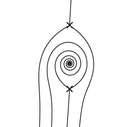
(g) .
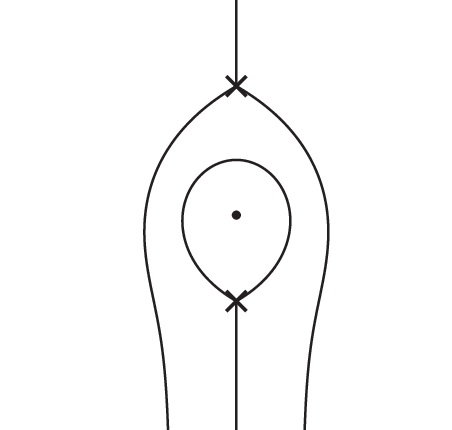
(h) .

(i) .
Here we recall some basic properties of the trajectories of from [Str84]. See also [BS13, Section 3] for comprehensible expositions. Firstly, the local foliation structure around simple zeros and poles of order are given below and depicted in Figures 4–6. For a simple zero , there are exactly three trajectories entering which are the Stokes curves (Figure 4). For a double pole , there are three cases depending on the residue (Figure 5).
- (a).
Clockwise or counterclockwise logarithmic spirals wrap onto . This occurs when .
- (b).
Radial arcs entering . This occurs when .
- (c).
Closed trajectories surround . This occurs when .
For a pole of order , there are exactly asymptotic tangent directions for the trajectories entering (Figure 6).
-1.73,-1)(1.73,2)
-1.5,-2.2)(9.5,1.5)
-1.5,-1.5)(1.5,1.5)
Secondly, we focus on global properties of the trajectories of . It is known that every trajectories fall into exactly one of the following five types ([BS13, Section 3.4]):
- (a).
A saddle trajectory flows into points in at both ends.
- (b).
A separating trajectory flows into a point in at one end, and a point in at the other end.
- (c).
A generic trajectory flows into points in at both ends.
- (d).
A closed trajectory is a simple closed curve in .
- (e).
A divergent trajectory has the limit set consisting of more than one point in at least one direction.
A Stokes curve is one of a saddle trajectory, a separating trajectory, and a divergent trajectory.
Saddle trajectories play important roles in this article. Typically, there are two kinds of saddle trajectories:
- (a).
A regular saddle trajectory connects two different points in . An example appears in Figure 3 (e).
- (b).
A degenerate saddle trajectory forms a loop around a double pole . An example appears in Figure 3 (h).
In addition to degenerate saddle trajectories, other kinds of loop-type saddle trajectories may appear. For example, a Stokes curve emanating from may return to the same point after encircling several points in . Such an example is discussed in [GMN13, Section 10], but we will not consider these cases. In this paper we will concentrate on the following cases:
Assumption 2.14.
The number of the saddle trajectories of is at most one.
Under Assumptions 2.3 and 2.14, a saddle trajectory must be either a regular or a degenerate saddle trajectory (see [BS13, Proposition 10.4]). Moreover, we can show that divergent trajectories never appear in this case.
Proof.
If does not have any saddle trajectory, then the statement is proved in [BS13, Lemma 3.1]. Assume that has a unique saddle trajectory. If a divergent trajectory appears, the interior of the closure of the divergent trajectory gives a domain called a “spiral domain”. It is known that the boundary of such a spiral domain must consist of a number of saddle trajectories (see [BS13, Section 3.4]). Since we have assumed that the number of saddle trajectories is exactly one, a domain whose boundary consists of saddle trajectories must be a “degenerate ring domain” (see [BS13, Section 3.4] or below). Then we have a contradiction because any trajectory in a degenerate ring domain must be a closed trajectory, which is not a divergent trajectory. ∎
Therefore, under Assumptions 2.3 and 2.14, a Stokes curve must be a saddle trajectory or a separating trajectory. In other words, a Stokes curve emanating from a turning point must flows into a point in , and these objects define a graph on .
Definition 2.16 ([KT05, Definition 2.10]).
- •
The Stokes graph of is a graph in whose vertices are the points in , and whose edges are the Stokes curves of . The Stokes graph is denoted by .
- •
The interior of each face of the Stokes graph is called a Stokes region of .
We sometimes write for the Stokes graph and call it the Stokes graph of when we want to emphasize the dependence on . If the Stokes graph does not have any saddle trajectory, is said to be saddle-free, and then is also said to be saddle-free, following [BS13, Section 3.5]. Under Assumptions 2.3 and 2.14, the Stokes regions of are classified as follows ([BS13, Section 3.4]):
- (a).
A horizontal strip is equivalent to a region
equipped with the differential . It is swept out by generic trajectories which connect two (not necessarily distinct) poles of arbitrary order .
- (b).
A half plane is equivalent to the upper half plane
equipped with the differential . It is swept out by generic trajectories which connect a fixed pole of order to itself.
- (c).
A degenerate ring domain is equivalent to a region
equipped with the differential for some . It is swept out by closed trajectories, and its boundary consists of a degenerate saddle trajectory and the double pole lying inside of the degenerate saddle trajectory.
For example, all three Stokes regions in Figure 3 (a) are half planes. On the other hand, all three Stokes regions in Figure 3 (c) are horizontal strips. In Figure 3 (b) there are five half planes near and two horizontal strips. An example of a degenerate ring domain can be found in Figure 3 (h).
In Section 2.8 we will explain the relationship between the geometry of the trajectories of and the Borel summability of the WKB solutions.
In the subsequent discussions we will consider not only the usual Borel resummation but also the Borel resummation in a direction as explained in Section 2.5. Lemma 2.12 shows that the Borel summability of the formal power series in the direction is equivalent to the Borel summability of . Actually, coincides with the formal power series (2.19) defined from the Schrödinger equation
| (2.38) |
(See Lemma 3.8 below.) Therefore, the Borel summability of (and of the WKB solutions) in the direction is relevant to the geometry of trajectories of the quadratic differential
| (2.39) |
Here is the original quadratic differential associated with . Since the quadratic differential also satisfies Assumption 2.3, trajectories of have the same properties explained in this subsection. Define the Stokes curves in the direction emanating from a turning point by
| (2.40) |
and also define the Stokes graph in the direction by the graph consists of the Stokes curves in the direction and the points in . The Stokes graph in the direction is denoted by .
If we vary the direction continuously, the topology of the Stokes graph changes when a saddle trajectory appears. Let us explain the phenomenon for an example defined on (see Figure 3 (d)–(f)). If and is sufficiently small, there are five Stokes regions; one is a horizontal strip and the other four are half planes (see in Figure 3 (d), (f)). As we vary continuously, the Stokes graph deforms continuously as long as . However, when , the horizontal strip disappears from the Stokes graph and the number of Stokes regions becomes four; all Stokes regions are half planes as shown in Figure 3 (e). Moreover, the topologies of the Stokes graphs for and are different. A similar change of the topology is also observed when a degenerate saddle trajectory appears (see Figure 3 (g)–(i)). These are typical examples of the phenomenon which we call the mutation of Stokes graphs. The mutation of Stokes graphs is the theme of the paper.
2.7 Orientation of trajectories
The inverse image of the foliation (2.36) in by the projection defines a foliation on . For a trajectory in , we call each lift of in by a trajectory in . Since the 1-form defined by is single-valued on , trajectories in has the orientation defined by the following rule; the real part of the function increases along the trajectory in the positive direction. Since the covering involution reverses the sign of , the orientation of a trajectories in is also reversed by . Figure 7 depicts examples of the orientation in the first sheet, projected to by . The orientation is well-defined on , but its projection has a discontinuity on the branch cut. When we discuss the orientation, we assign the symbols and to the asymptotic directions of trajectories entering points of so that the trajectories with positive directions flows from to . These signs depend on the choice of the branch cuts and embedding , and the covering involution exchanges all signs simultaneously.
0.5,-3)(16,3)
2.8 Borel summability of WKB solutions
Now we claim an important result concerning with the Borel summability of the WKB solutions for a fixed direction . Note that, setting in the following claims, we obtain results for the “usual” Borel summability (Definition 2.10).
Let be the quadratic differential associated with , and assume that has at most one saddle trajectory. Let be the Stokes graph in the direction in Section 2.6. Take any Stokes region of . Recall that must be one of a horizontal strip, a half plane or a degenerate ring domain. Fix a local coordinate of whose domain contains the Stokes region . Recently, Koike and Schäfke proved the following statement which ensures the Borel summability of the formal power series on each Stokes region when is the Riemann sphere .
Theorem 2.17 ([KS]).
Assume that is the Riemann sphere , and the coefficients of the potential function of (2.1) are meromorphic functions satisfying Assumption 2.5. Let and be as above.
- (a).
For any fixed , the formal power series is Borel summable in the direction as a formal power series in . The Borel sum of becomes holomorphic function of around the point in question (and also analytic in on ).
- (b).
Let be any pole lying on the boundary of . Then, for any fixed , the formal power series defined by the integral
(2.41) is Borel summable in the direction as a formal power series in if the path of the integral (2.41) is contained in . The Borel sum becomes holomorphic function of around the point in question (and also analytic in on ).
Actually, the above claim follows from the results of [KS] and the fact that is integrable at each pole (see Proposition 2.8). In [KS] the above claim is proved in the case . The statement for general follows from the result of [KS] together with Lemma 2.12 (see Section 2.6). Although Theorem 2.17 is proved when in [KS], their proof is also applicable to the case when is a compact Riemann surface since their proof uses only local properties of in each Stokes region and the orders of poles lying on the boundary of . Therefore, we can extend it to the following theorem.
Theorem 2.18.
Theorem 2.17 also holds for any compact Riemann surface .
Since Stokes regions are independent of the choice of the local coordinate, the notion of Borel summability is also independent of the choice. If lies on a Stokes curve in the direction , the trajectory of passing through flows into a turning point at one end. The proof of Theorem 2.17 by [KS] is not applicable to such a situation.
Next we discuss the Borel summability of the WKB solutions in a fixed direction . Since the WKB solutions are defined by integrating along a path on the Riemann surface , the Borel summability of the WKB solutions is more delicate than that of explained above. To state the criterion of the Borel summability of the WKB solutions proposed by Koike and Schäfke, we introduce the notion of an admissible path. Set , and .
Definition 2.19.
A path on is said to be admissible in the direction if the projection of to by either never intersects with the Stokes graph , or intersects with only at points in .
Especially, any generic trajectory and any closed trajectory of are admissible in the direction . For a given path on which is not admissible, we may find a decomposition of the path into a finite number of admissible paths as follows.
Lemma 2.20.
Let be a path on with end-points satisfying the following conditions:
- •
The end-point either does not lie on the Stokes graph or a point in . The other end-point also satisfies the same condition.
- •
never intersects with a saddle trajectory of .
Then, has a decomposition into a finite number of paths in the relative homology group and each summand () is admissible in the direction .
Proof.
In the proof we regard a Stokes region as one of its lift in by the projection . Although two Stokes regions in have the same projection, we distinguish them if they lie on different sheets of . Moreover, since we only consider the Stokes graph for a fixed , we omit “in the direction ” for simplicity.
Since any point in a Stokes region and a point in which lies on the boundary of the Stokes region can be connected by an admissible path, in the proof we may assume that never passes through a point in (i.e., is contained in ) without loss of generality. Especially, we may assume that . If , and the path are contained in the same Stokes region, is admissible by definition. Therefore, it suffices to consider the case that and are contained in different Stokes regions and the path connects them crossing finitely many Stokes curves which are not saddle trajectories. We may also assume that the Stokes regions containing or are not degenerate ring domains (otherwise a path satisfying the assumption never exists).
Let us consider the case that intersect with a Stokes curve just once. Since the Stokes curve is not a saddle trajectory, it must be a separating trajectory by Lemma 2.15. That is, the Stokes curve connects a point and a point . Therefore, we can decompose into a sum of two paths in the relative homology group, where (resp., ) connects (resp., ) and as indicated in Figure 8. Here we can take the path (resp., ) to be admissible since the point lies on the boundary of the Stokes region containing (resp., ).
Any path in can be written by the sum of a finite number of paths whose each summand intersect with the Stokes curves just once. Therefore, applying the decomposition as in Figure 8 to each summand, we can find a desired decomposition of by admissible paths. ∎
-2.2,-1.5)(6,1.5)
Then, a criterion of the Borel summability of the WKB solutions proposed by Koike and Schäfke is stated as follows.
Corollary 2.21 ([KS]).
- (a).
Let be a path on with end-points satisfying the same assumption in Lemma 2.20. Then, the formal power series is Borel summable in the direction .
- (b).
If the Stokes graph is saddle-free, then the WKB solutions which are normalized as (2.26) and (2.28) are Borel summable in the direction at any point in each Stokes region. The Borel sums of the WKB solutions give analytic solutions of (2.1) on each Stokes region (which is also analytic in on a domain ).
Proof.
Theorem 2.17 (b) ensures that a formal power series defined by integrating along an admissible path is Borel summable in the direction . Therefore, the first claim (a) follows from Lemma 2.20.
Let us show the claim (b). When the Stokes graph is saddle-free, any path on can be decomposed into admissible paths by Lemma 2.20. For example, if lies on a Stokes region, then the path (see Figure 2) which determines the WKB solutions (2.26) is decomposed into admissible paths as depicted in Figure 9. Therefore the integral is Borel summable in the direction by Theorem 2.17 (b). The Borel summability of the WKB solutions (2.26) follows from (c) in Proposition 2.11. The Borel summability of the WKB solutions (2.28) can be shown similarly. ∎
-0.5,-2)(8,2)
Remark 2.22.
Suppose that the Stokes graph has a saddle trajectory. Even if the point does not lie on the Stokes graph, the path in Figure 2 can not be decomposed into admissible paths when intersects with the saddle trajectory. Therefore, we can not expect the Borel summability for the WKB solutions in general when a saddle trajectory appears in the Stokes graph.
The above statements guarantee the Borel summability of and the WKB solutions in a fixed direction . As is explained in Section 2.5, the rotation of the direction may break the Borel summability of the WKB solutions. The following claim gives an criterion for the invariance of the Borel sum under a rotation of .
Proposition 2.23.
Let be a path on with end-points . Suppose that there exist real numbers with such that the following conditions hold.
- •
The quadratic differential has at most one saddle trajectory for any .
- •
The end-point either does not lie on the Stokes graphs for any or is a point in . The other end-point also satisfies the same condition.
- •
The path never touches with a saddle trajectory of for any .
Then, the Borel sums of the formal power series in the direction and coincide. That is, the following equality holds as analytic functions of defined on a domain containing :
| (2.42) |
Proof.
Since satisfies the assumption of Corollary 2.21 (a) for any satisfying , the formal power series is Borel summable in all directions . That means that the Borel transform of does not have singular points in a domain containing the sector , and has an exponential growth near (see Definition 2.10). Hence, the Laplace integrals (2.32) give the same analytic function of for all . Thus we obtain (2.42). ∎
Remark 2.24.
The “resurgence property” (i.e., the endlessly continuability of the Borel transform), which is stronger than the Borel summability, was claimed by Ecalle in [Eca84], but not all details are clear (see [DP99, Comment in Section 1.2]). Still currently there are many contributions to warrant the resurgence property of the WKB solutions; e.g., [Get09, Get11, GT11]. The case where the potential function is entire on is discussed in these works.
2.9 Connection formula for WKB solutions
Corollary 2.21 (b) ensures that, if the Stokes graph in a fixed direction is saddle-free, then the WKB solutions are Borel summable in the direction on each Stokes region of . Here we show an explicit and simple connection formula between the Borel sums of the WKB solutions defined on adjacent Stokes regions found by Voros [Vor83]. (In this subsection we do not consider the rotation of the direction . The following statements hold for any fixed , if the Stokes graph is saddle-free.)
Here we specify the situation to state the connection formula. Assume that the Stokes graph is saddle-free. Let be a simple turning point, and suppose that two Stokes regions and have a common boundary which is a Stokes curve emanating from , and comes next to in the counter-clockwise direction with the reference point . Take appropriate branch cuts so that does not cross any branch cut. Then we have two possibilities (a) and (b) shown in Figure 10 for the sign of the other end-point of than . For each case, the connection formula is formulated as follows.
0,-3)(12,3)
Theorem 2.25 ([Vor83, Section 6], [AKT91, Section 2]).
Suppose that the Stokes graph is saddle-free. Let , , and be as above and
be the WKB solutions normalized at the turning point as defined in (2.26). Denote by () the Borel sum of on the Stokes region (). Then, the analytic continuation of to across the Stokes curve satisfy the following equalities:
| (2.43) | |||
| (2.44) |
Here appearing in the formula is the imaginary unit .
Remark 2.26.
Theorem 2.25 is proved by [Vor83] and [AKT91] in the case that . Since the proof of [AKT91, Appendix A.2] is based only on local properties of the WKB solutions near a simple turning point, the same discussion is applicable to a general compact Riemann surface . Therefore, together with Theorem 2.18, Theorem 2.25 is valid when is a general compact Riemann surface.
Remark 2.27.
Theorem 2.25 gives connection formulas which describe the analytic continuation of the Borel sums of WKB solutions on the -plane. On the other hand, the formulas indeed describe the Stokes phenomenon (for a large ) occurring to WKB solutions since they are derived through the analysis of the singularity of the Borel transforms of WKB solutions (see [KT05]). That is, we can reformulate Theorem 2.25 in an alternative manner as follows: Take any point , and suppose that there exists a direction and a sufficiently small number satisfying
- •
Stokes graphs in any direction satisfying is saddle-free,
- •
the point lies on a Stokes curve in the direction , and does not lie on the Stokes graph in any direction satisfying or .
Let be the WKB solution normalized at the turning point from where the Stokes curve emanates, and denote by (resp., ) the Borel sum of in the direction (resp., ) Then, the following relation holds in a neighborhood of .
| (2.45) | |||
| (2.46) |
Thus, the Stokes phenomenon occurring to is described by the completely same formulas in Theorem 2.25. We use this point of view in Appendix B.
The connection formula in Theorem 2.25 is quite effective for the global problems of differential equations. For example, if and the equation is Fuchsian (i.e., all poles of are order 2) with a saddle-free Stokes graph, then the monodromy group of can be expressed by the following quantities ([KT05, Theorem 3.5]):
- (i)
characteristic exponents at regular singular points,
- (ii)
the Borel sum of contour integrals of along cycles in .
In [KT05, Section 3.1] a recipe to obtain an explicit expression of the monodromy group is given. Contour integrals of appear when we use the connection formulas (2.43) and (2.44) iteratively.
3 Voros symbols and Stokes automorphisms
In this section we introduce an important notion in the exact WKB analysis, called the Voros symbols. We discuss the jump property of the Voros symbols caused by the Stokes phenomenon relevant to the appearance of saddle trajectories in the Stokes graph.
3.1 Homology groups and Voros symbols
Let us consider the homology group and the relative homology group . In what follows we call elements of and as cycles and paths, respectively, to distinguish them. By the Lefschetz duality there exists a bilinear form
| (3.1) |
on these homology groups given by the intersection number of cycles and paths. The intersection number depends on the orientations of cycles and paths, and we normalize the bilinear form as -axis, -axis. It also induces a bilinear form
| (3.2) |
We call both these bilinear forms intersection forms.
Here we introduce the notion of the Voros symbols, which are the main objects in this paper.
Definition 3.1 ([DDP93, Section 1.2]).
- •
Let be a path. The formal power series is called the Voros symbol for the path . Here is the formal power series defined by the integral
(3.3) - •
Let be a cycle. The formal series is called the Voros symbol for the cycle . Here is the formal series defined by the integral
(3.4)
Remark 3.2.
The Voros symbols for are formal power series without a exponential factor since is a formal power series. On the other hand, the Voros symbols for are formal series with the exponential factors , where
| (3.5) |
As mentioned in Section 2.9, the Voros symbols appear in the expression of monodromy group of the equation (2.1) (see Section 2.9). They are Borel summable (in the direction ) if the paths of the integrals in (3.3) and (3.4) do not intersect with a saddle trajectory of by Corollary 2.21. The appearance of a saddle trajectory breaks the Borel summability, and cause the Stokes phenomenon as explained in Section 2.5. That is, if a saddle trajectory appears, the Borel sums of a Voros symbol in the directions are different in general for a sufficiently small . As noted in Section 2.6, the Stokes graph mutates when a saddle trajectory appears. The rest of this section is devoted to analyze the Stokes phenomenon occurring to the Voros symbols under the mutation of Stokes graphs.
3.2 Saddle class associated with saddle trajectory
Suppose that the Stokes graph has a regular or degenerate saddle trajectory . Recall that a regular saddle trajectory connects two different zeros of , while a degenerate saddle trajectory forms a closed loop around a double pole of (see Section 2.6). Then, there exists a cycle whose projection on by surrounds as in Figure 11, and its orientation is given so that
| (3.6) |
(See Section 2.7 for the rule of the assignment of signs.) Note that, if a cycle satisfies the above conditions, then the cycle also satisfies the same conditions. (Here is the image of by the covering involution .) We choose any of the two cycles, and call the resulting homology class the saddle class associated with the saddle trajectory , following [BS13, Section 3.6]. Note that “the Voros symbol for the saddle class” is well-defined because
| (3.7) |
holds for any cycle due to the anti-invariant property (2.25) of .
5.5,-2.5)(16.5,2.5)
3.3 Saddle reduction
0.5,-9)(16,2.3)
Suppose that the Stokes graph has a unique regular or degenerate saddle trajectory . Then, as in [BS13, Section 5 and Section 10.3], there exists such that for all the quadratic differentials are saddle-free. We call saddle reductions of . The topology of the Stokes graph (resp., ) does not change as long as since (resp., ) is saddle-free for all . However, varying across , the topology of the Stokes graph changes as explained in Section 2.6. We say that and are related by a flip (resp., pop) if they give saddle reductions of a regular (resp., degenerate) saddle trajectory (see Figure 12).
Since the Stokes graphs are saddle-free, the Voros symbols are Borel summable in any direction with by Corollary 2.21. Furthermore, we can show the following.
Lemma 3.3.
Suppose that the Stokes graph has a unique saddle trajectory. Then, there exists a sufficiently small such that the following equalities hold as analytic functions of for any :
| (3.8) | |||||
| (3.9) |
Here and are any path and cycle, respectively.
Proof.
Note that any path or any cycle is decomposed into the sum of a finite number of paths whose end-points are contained in in the relative homology group (see Figure 13). Therefore, it suffices to show the equalities (3.8) and (3.9) for any whose end-points are contained in . Take any such a path , and fix a sufficiently small so that the Stokes graphs are saddle-free for all . Then, the path never touches with saddle trajectory of for all . Therefore, since satisfies the assumption of Proposition 2.23, the equalities (3.8) and (3.9) follows form (2.42). ∎
5,-2.3)(18,2.3)
Define (resp., ) by the Borel sum (resp., ) of the Voros symbol for a path (resp., for a cycle ) for a sufficiently small . Due to Lemma 3.3, and are well-defined. As explained in Section 2.5, the Borel sums and are analytic in on a domain containing . In the rest of this section we will describe the relationship between (resp., ) and (resp., ); that is, the formulas describing the Stokes phenomenon occurring to the Voros symbols.
3.4 Jump formula and Stokes automorphism for regular saddle trajectory
Here we specify the situation to state Theorem 3.4 below. Suppose that the Stokes graph has a unique regular saddle trajectory with the associated saddle class . Let be saddle reductions of for a sufficiently small as in (a) of Figure 12 (i.e., and is related by a flip). Then, the Stokes phenomenon occurring to the Voros symbols are described explicitly by the following “jump formula”.
Theorem 3.4 ([DDP93, Section 3]).
The Borel sums and for any and any satisfy the following equalities as analytic functions of on a domain containing :
| (3.10) | ||||
Remark 3.5.
Originally, Theorem 3.4 is proved in [DDP93, Section 3] for the case that the potential is independent of and is a polynomial in . Since the Borel summability of the WKB solutions are established in [KS] (see Theorem 2.17 and 2.18), the proof of [DDP93] is also valid for general cases. For a convenience of readers, we briefly recall the sketch of the proof of Theorem 3.4 in Appendix A.
The formula (3.10) in fact describes the Stokes phenomenon for the Voros symbols relevant to the flip of the Stokes graph. The exponentially small difference between the Borel sums of Voros symbols are explicitly given in (3.10). Note that the Borel sum is exponentially small for a sufficiently large because it is asymptotically expanded to the formal series as whose exponential factor is exponentially small due to the orientation (3.6) of the saddle class .
In [DDP93] the formula (3.10) is stated in a different manner. Let be the field of the rational functions generated by the Voros symbols and , which we call the Voros field for a potential . Define a field automorphism by
| (3.11) |
The equalities (3.10) implies that satisfies
| (3.12) |
Here is the Borel summation operator for a sufficiently small . To be precise, the map in Definition 2.10 is not defined for sums of Voros symbols with different exponential factors. Here we extend it to the map from to a space of analytic functions of so that commutes with the operations addition, multiplication, and division. In view of (3.12), the map measures the difference between the Borel sums of Voros symbols for different directions. The map is called the Stokes automorphism for the saddle class associated with a regular saddle trajectory (see [DP99, Section 0.4]).
We call the formulas (3.10) and (3.11) the DDP (Delabaere-Dillinger-Pham) formula. Later in Section 7 we will reformulate the DDP formula in view of cluster algebras theory. Furthermore, we apply this formulation to study identities of Stokes automorphisms.
Remark 3.6.
The DDP formula resembles to the Kontsevich-Soibelman transformation in [GMN13], where the counterpart of the Voros symbols are the Fock-Goncharov coordinates of the moduli space of the flat connections associated with a Hitchin system of rank 2. In their context, a quadratic differential appears as the image of the Hitchin fibration, and its saddle trajectories capture BPS states in a four dimensional field theory.
3.5 Jump formula and Stokes automorphism for degenerate saddle trajectory
Similarly to regular saddle trajectories, degenerate saddle trajectories also cause the Stokes phenomenon for the Voros symbols. This subsection is devoted to the description of the formula for the Voros symbols describing the Stokes phenomenon. Suppose that the Stokes graph has a unique degenerate saddle trajectory with the associated saddle class . Let be saddle reductions of for a sufficiently small as in (b) of Figure 12 (i.e., and is related by a pop). Then, the Stokes phenomenon occurring to the Voros symbols are described explicitly the following jump formula.
Theorem 3.7 ([AIT]).
The Borel sums and for any and any satisfy the following equalities as analytic functions of on a domain containing :
| (3.13) | ||||
The formula (3.13) is derived as a corollary of the main result of the forthcoming paper [AIT]. To make the paper self-contained, we will give an alternative proof of (3.13) in Appendix B. Note that the Borel sum of the Voros symbol do not jump for any . This is a consequence of the first equality of (3.13) and the fact for any .
Moreover, we have
| (3.14) | ||||
since is holomorphic at the double pole by Proposition 2.8. This implies that the Voros symbol for the saddle class associated with a degenerate saddle trajectory is not a formal series but a scalar.
Similarly to (3.11), we also define a field automorphism by
| (3.15) |
Then the map satisfies
| (3.16) |
The map is called the Stokes automorphism for the saddle class associated with a degenerate saddle trajectory .
3.6 -action on potential and jump formulas
Let us give an alternative interpretation of the jump formulas (3.10) and (3.13) in view of the deformation of the potential . We consider a particular deformation realized by an action of the unit circle , which we call the -action on the potential .
Suppose that the Stokes graph has a unique regular or degenerate saddle trajectory . Take a number and consider the family of Schrödinger equations
| (3.17) |
Here the family of potentials is defined by
| (3.18) |
where is the original potential of (2.1). We call this family the -family for the potential . Note that (3.18) satisfies Assumptions 2.3 and 2.5 for all . Taking sufficiently small, we may assume that the Stokes graph defined from is saddle-free if , . Since the principal terms of potentials satisfy
| (3.19) |
the quadratic differential associated with (3.17) is noting but defined in (2.39). The Stokes graph for coincides with the original Stokes graph containing the saddle trajectory .
For any fixed , let (resp., ) be the formal power series defined in the same manner as (2.14) (resp., (2.19)) from the Schrödinger equation (3.17). The following statement immediately follows from the uniqueness of formal solutions of the Riccati equation associated with (3.17) (see Section 2.3).
Lemma 3.8.
The following identities holds:
| (3.20) |
We define the Voros symbols and (, ) of the Schrödinger equation (3.17) by
| (3.21) |
Note that, by (3.19), the Riemann surface defined from (3.17) does not depend on . Thus, the homology groups and for the Schrödinger equations (3.17) also do not depend on . Thus, the equality (3.20) implies that
| (3.22) |
hold as formal series.
Lemma 3.9.
For any satisfying , the formal series and are Borel summable (in the direction ), and the equalities
| (3.23) |
hold as analytic functions of on .
Proof.
Since the argument is the same, let us concentrate on the case of . It follows from (2.35) that the equality
holds near . Here and are the Borel transform of and , respectively. Since the quadratic differential is saddle-free, is Borel summable in the direction by Corollary 2.21. Then, Lemma 2.12 implies that is Borel summable in the direction and we have the equality
| (3.24) |
by the definition (2.33) of the Borel sum in the direction . Then the desired equality (3.23) follow from (3.24). ∎
The equality (3.23) and Lemma 3.3 imply that the limit of the function exists and coincides with defined in Section 3.3. That is,
| (3.25) |
holds on . Similarly, we also have
| (3.26) |
Therefore, we obtain the following jump formulas for the -action on the potential from Theorem 3.4 and 3.7.
Theorem 3.10.
- (a).
Suppose that is a regular saddle trajectory with the associated saddle class . Then we have
(3.27) for any and any .
- (b).
Suppose that is a degenerate saddle trajectory with the associated saddle class . Then we have
(3.28) for any and any .
4 Cluster algebras with coefficients
In this section we summarize the basic notions and properties in cluster algebras which we will use in this paper. We also introduce the notion of signed mutations of seeds in Section 4.6 to accommodate the forthcoming results of this paper. We ask the readers to consult [FZ07, Nak12], for example, for further explanations if necessary, though it is our hope that the readers will not be bogged down in the cluster algebras machinery presented in this and the next sections, and smoothly proceed to Section 6 where our real work starts.
4.1 Semifields
Let us start from the notion of semifields, where “coefficients” of cluster algebras live.
Definition 4.1.
A semifield is a multiplicative abelian group endowed with an addition denoted by , which is commutative, associative, and distributive with respect to the multiplication.
To say it plainly, a semifield is almost a field, but without zero and subtraction. In this paper we mainly use the following examples.
Example 4.2.
Let be an -tuple of formal variables.
(a) The universal semifield of . This is the semifield of all nonzero rational functions of which have subtraction-free expressions, where the multiplication and the addition are defined by the usual and in the rational function field of . As a standard example, the polynomial does not seem to belong to ; however, it actually does, since
| (4.1) |
(b) The tropical semifield of . This is the multiplicative free abelian group generated by , endowed with the tropical sum defined by
| (4.2) |
It is called so because it is essentially the exponential and multivariable version of the tropical semiring (also known as the min-plus algebra) , . The tropical semiring is the central object of the tropical mathematics well studied since 90’s. See [SS09] for the subject and the explanation for this peculiar terminology.
For a given semifield , let denote the group ring of over . Namely, is the commutative ring of all formal finite sums (). Note that we have two kinds of additions, for and the addition for the group ring. For , there is no subtraction, but for , there is the usual subtraction in . It is known that is a domain [FZ02, Section 1.2]; namely, it has no zero divisors. Thus, the field of fractions of the ring is well-defined.
4.2 Mutation of seeds and cluster algebra with coefficients
To introduce a cluster algebra (with coefficients), let us first fix a positive integer called the rank, and a semifield called the coefficient semifield. We choose an -tuple of formal variables, say, , and consider the field of the rational functions in with coefficients in , which denoted by .
A (labeled) seed with coefficients in is a triplet with the following data:
- •
an exchange matrix , which is a skew-symmetric integer matrix,
- •
a cluster , which is an -tuple of algebraically independent elements in over ,
- •
a coefficient tuple , which is an -tuple of elements in .
Each and are called a cluster variable and coefficient, respectively. In this paper we call them, a little casually, an -variable and a -variable, respectively. (They correspond to an -coordinate and an -coordinate in [FG09a], respectively.)
For any seed and any , we define another seed , called the mutation of at and denoted by , by the following relations:
| (4.5) | ||||
| (4.6) | ||||
| (4.7) |
Here, for any integer , we set . The above relations are called the exchange relations. The involution property holds.
Definition 4.3.
Let us fix an arbitrary seed with coefficients in , and call it the initial seed. Then, repeat mutations from the initial seed to all directions. Let denote the set of all so obtained seeds, including the initial one; namely,
| (4.8) |
The cluster algebra with coefficients in is the -subalgebra of generated by all -variables belonging to seeds in . A seed in is called a seed of .
What is important in our application is not the algebra itself but the exchange relations (4.5)–(4.7). They are the abstraction of relations occurring in Lie theory due to Fomin and Zelevinsky. For example, the relation (4.7) typically appears as relations in the coordinate rings of certain algebraic varieties related to Lie group, e.g., Grassmannians, , etc. The relation (4.6) is a sort of the “dual” of the relation (4.7) as we see below. As explained at the beginning of Section 1, it is nowadays known that the cluster algebra structure, (i.e., the exchange relations (4.5)–(4.7)) serves a common underlying algebraic/combinatorial structure in several branches of mathematics — from algebra, geometry, analysis to combinatorics. Such ubiquity as a common structure reminds us of root systems. Indeed, cluster algebra theory may be regarded as an extended theory of root systems in several aspects. An explicit example of the exchange relations (4.5)–(4.7) will be exhibited in Example 4.10 later.
For each seed with coefficients in , we define -variables by
| (4.9) |
It is easy to verify the following property by using (4.5)–(4.7).
Proposition 4.4 ([FZ07, Prop. 3.9]).
Under the mutation the following relation holds:
| (4.10) |
In other words, -variables mutate just in the same way as -variables.
4.3 Quivers
It is often convenient to represent a skew-symmetric matrix by a (labeled) quiver whose vertices are labeled by . In our convention, we write arrows from vertex to vertex if and only if . This gives a one-to-one correspondence between skew-symmetric matrices and quivers without any loops (1-cycles) and oriented 2-cycles. Here is an example:
| (4.11) |
In terms of quivers, the exchange relation (4.5) for the mutation at is translated as follows.
-
Step 1. For each pair of an arrow from to and an arrow from to , add an arrow from to .
-
Step 2. Reverse all arrows incident with .
-
Step 3. Remove the arrows in a maximal set of pairwise disjoint 2-cycles.
For example, for the quiver in (4.11), the mutation at is done in the following manner.
| (4.12) |
4.4 Tropicalization of -variables and tropical sign
In this paper we mainly use the following two choices of -variables. (See Example 4.2.)
- (a).
We set the coefficient semifield as with ; furthermore, we set the initial -variables as . We call the -variables of the universal -variables.
- (b).
We set the coefficient semifield as with ; furthermore, we set the initial -variables as . We call the -variables of the tropical -variables. (It is more standard to call them the principal coefficients [FZ07], but here we emphasize their tropical nature.)
The tropical -variables are obtained from the universal -variables by applying the tropicalization map in Example 4.2,
| (4.13) |
Namely, for any universal -variable , let . Since is a semifield homomorphism, it preserves the exchange relation (4.6); therefore, it commutes with mutations. Thus, is a tropical -variable. From now on we conveniently use this expression for tropical -variables.
By definition, a tropical -variable is a Laurent monomial of the initial tropical -variables ; namely, it is written in the form
| (4.14) |
where is an integer vector depending on . The vector is introduced in [FZ07] and called the -vector of .
We say that an integer vector is positive (resp., negative) if it is a nonzero vector and its components are all nonnegative (resp., nonpositive). We have the following important property of -vectors.
Theorem 4.5 (Sign coherence of -vectors ([FZ07, Prop. 5.7], [DWZ10, Theorem 1.7])).
Any -vector is either a positive vector or a negative vector.
Thanks to the theorem, we have the notion of the tropical sign.
Definition 4.6.
Let be a cluster algebra with universal -variables, and let be its seed. Then, to each component of we assign the tropical sign as (resp., ) if the -vector is positive (resp., negative).
Throughout the paper we conveniently identify the signs and the numbers .
It is important that the tropical sign is a relative concept depending on and the initial seed . By the definition of the tropical sign, we have
| (4.15) |
in .
4.5 -expression of exchange relations
Let us focus on some fine property of the exchange relations (4.6) and (4.7). It is easy to check that (4.6) and (4.7) can be expressed alternatively as [Kel11, Nak12]
| (4.16) | ||||
| (4.17) |
where , and the right hand sides are independent of the choice of . We call them the -expression of the exchange relations.
Let us specialize the -variables in (4.16) and (4.17) to tropical -variables ; furthermore, let us specialize therein to the tropical sign . Then, by (4.15), the relations (4.16) and (4.17) reduce to the following ones:
| (4.18) | ||||
| (4.19) |
where . These are an alternative expressions of the exchange relations for tropical -variables and -variables with tropical -variables as coefficients.
4.6 Signed mutations
We introduce some new notions in cluster algebras, motivated by the forthcoming results in this paper.
For any seed with coefficients in , any , and any sign , we introduce the signed monomial mutation by the following exchange relation, where is defined as usual:
| (4.20) | ||||
| (4.21) |
Unlike (4.18) and (4.19), they depend on . If we set to the tropical sign for the universal -variables, the relation (4.20) reduces to the exchange relation (4.18) of the tropical -variables. Starting from a given initial seed , we obtain a family of seeds by repeating the above mutations to any direction and any sign . We call so obtained ’s and ’s the monomial -variables and the monomial -variables, respectively.
In the same setting of seeds, we also consider another kind of mutation, the signed mutation , by keeping (4.20) and replacing (4.21) by the following:
| (4.22) |
where . Again, it depends on . If we set to the tropical sign of the universal -variables, then the relation (4.22) reduces to the exchange relation (4.19) of -variables with tropical -variables as coefficients.
We have a natural extension of Proposition 4.4.
Proposition 4.7.
The proof can be done in a similar (and a little easier) calculation as for Proposition 4.4. However, the result is new in the literature.
4.7 Periodicity in cluster algebras
Let us introduce the notion of periodicity in a cluster algebra. We call a sequence with a mutation sequence, and we naturally identify it with the sequence (composition) of mutations .
Theorem 4.8.
Let be a cluster algebra with universal -variables, and let be a mutation sequence. Let and be seeds of such that , and let be a permutation of . Then, the following conditions are equivalent.
(a). , , and hold for any and .
(b). holds for any .
(c). holds for any .
(d). holds for any .
(e). holds for any , where is the one obtained from by the tropicalization of -variables.
Proof.
Definition 4.9.
A mutation sequence is called a -period of if one of the conditions (a)–(e) in Theorem 4.8 holds for the seed .
Many interesting examples of periodicities of seeds are known [FZ07, Kel10, IIK+13a, IIK+13b, NS12]. Here, we give the simplest example, which will be used as the running example throughout the paper.
Example 4.10 (Pentagon relation (1)).
Consider the cluster algebra whose initial exchange matrix and the corresponding quiver are given by
| (4.24) |
This is the cluster algebra of type in the classification of [FZ02]. In particular, it is of finite type, namely, there are only finitely many seeds. Set to be the initial seed , and consider the mutation sequence , i.e.,
| (4.25) |
For simplicity, we write the initial variables and . According to (4.9), we set the initial -variables as
| (4.26) |
Then, using the exchange relations (4.6) and (4.17), we obtain the following explicit form of seeds:
Here, the encircled vertices in quivers are the mutation points in the sequence (4.25). We see that the mutation sequence is a -period of , where is the permutation of and . This periodicity is known as the pentagon relation. The tropical -variables at the mutation points are
| (4.27) |
and the corresponding tropical signs are
| (4.28) |
5 Surface realization of cluster algebras
There is a class of cluster algebras which can be realized (in various sense) by triangulations of surfaces [GSV05, FG06, FST08, FT12]. This construction is often referred to as the surface realization of cluster algebras. Since careful treatment of mutations involving a self-folded triangle is crucial throughout the paper, we explain in detail how there are related to tagged triangulations and signed triangulations. We mostly follow [FST08, FT12], but we do some reformulation to work with labeled triangulations. The extended seeds and their signed mutations and pops are also defined.
5.1 Ideal triangulations of bordered surface with marked points
To start, we choose a compact connected oriented surface possibly with boundary , and a finite set of marked points on that is nonempty and includes at least one marked point on each boundary component and possibly some interior points. If a marked point is an interior point of , then it is called a puncture. We impose the following assumption by a technical reason [FST08]:
Assumption 5.1.
The following cases of are excluded:
- •
a sphere with less than four punctures,
- •
an unpunctured or once-punctured monogon,
- •
an unpunctured digon,
- •
an unpunctured triangle.
In the above a surface homeomorphic to a disk with marked points on the boundary is called a polygon, and, in particular, monogon, digon, triangle for , respectively.
A pair satisfying Assumption 5.1 is called a bordered surface with marked points, or a bordered surface, for simplicity.
Remark 5.2.
First we consider triangulations of by ordinary arcs, where “ordinary” means “not tagged” which will be introduced later.
Definition 5.3.
An arc in a bordered surface is a curve in such that
- •
the endpoints of are marked points,
- •
does not intersect itself except for the endpoints,
- •
is away from punctures and boundaries except for the endpoints,
- •
is not contractible into a marked point or onto a boundary of .
Furthermore, each arc is considered up to isotopy in the class of such curves. For example, “distinct (resp. identical) arcs” means distinct (resp. identical) isotopy classes of curves unless otherwise mentioned.
Two arcs are said to be compatible if there are representatives in their respective isotopy classes such that they do not intersect each other in the interior of .
Definition 5.4.
An ideal triangulation of is a maximal set of distinct pairwise compatible arcs in .
See Figure 14 for examples of ideal triangulations. We also put labels 1, 2, …to the arcs for the later use. As in the second example, some degenerate triangles, such as self-folded triangles (e.g., 4-5) and triangles with identified vertices (e.g., 2-3-4), may appear around a puncture. From now on we also call them triangles (of an ideal triangulation).
-1,-2)(1,1.6) -1,-2)(1,1.2)
Definition 5.5.
For an ideal triangulation of and an arc , if there is another arc such that that is an ideal triangulation, then is called a flip of , and is called a flip of at . (As wee see soon, such is unique for each if it exists.)
Now we encounter a problem that not all arcs are flippable. For example, in the triangulation in Figure 14 (b), the arc with label 5 is not flippable. Luckily this is the only situation where an arc is not flippable. Indeed, if an arc is the inner side of a self-folded triangle (an inner arc, for short), it is not flippable. Otherwise, is the common side of two (possibly degenerate) triangles. These triangles make a quadrilateral such that is one of its diagonal. Then, is uniquely flipped to another diagonal of the same quadrilateral, and vice versa. See Figure 15. In particular, the uniqueness of the flip was also shown.
-1,-1.2)(1,1.2) -1,-1.2)(1,1.2) -1,-1.2)(1,1.2)
For a given bordered surface it is known that all ideal triangulations are connected by a sequence of flips [Hat91]. In particular, they share the same cardinality of arcs. For an ideal triangulation with , one can label the arcs in by the set as in Figure 14. We call it a labeled ideal triangulation, and we still write it as . In other words, a labeled ideal triangulation is not simply a set of arcs; rather, it is an -tuple of arcs , where is the arc with label . A flip of an (unlabeled) ideal triangulation induces a flip of a labeled ideal triangulation by preserving the labels of the unflipped arcs. Suppose that and are labeled ideal triangulations. Then, if is a flip of at , then is also a flip of at . and for . So, we can write them as and , like the mutation in cluster algebras, and call them the flip at .
Definition 5.6.
To each labeled ideal triangulation of with , we assign a skew-symmetric matrix , called the (signed) adjacency matrix of , as follows.
(a). The case when neither nor are inner arcs in . First, for any triangle in which is not self-folded, we define
| (5.1) |
Then, we define
| (5.2) |
where the sum runs over all triangles in which are not self-folded.
(b). The rest of the case. For an inner arc in , let be the outer side of the self-folded triangle which belongs to. Then, we define
| (5.3) |
where the right hand side is defined in (5.1).
Example 5.7.
The following fact is a key to connect triangulations and cluster algebras.
Theorem 5.8 ([FG07, GSV05]).
Let be a labeled ideal triangulation of , and let not be an inner arc in . Then, .
The theorem says that the flip of labeled ideal triangulations and the mutation of the corresponding skew-symmetric matrices (equivalently, quivers) in (4.5) are compatible, if the targeted arc is flippable. However, recall that the inner arcs are not flippable, while skew-symmetric matrices can be mutated to any direction. See Figure 16 for an illuminating example of a digon with a puncture in some ideal triangulation. Fomin, Shapiro, and Thurston [FST08] remedied this discrepancy by introducing the tagged triangulations.
-1,-1.2)(3.3,1.2) 0,0)(1,1) 0,0)(1,1) -1,-1.2)(3.3,1.2) -1,-1.2)(3.3,1.2) 0,0)(1,1) 0,0)(1,1) -1,-1.2)(3.3,1.2)
5.2 Tagged triangulations
For each arc in a bordered surface , cut into three pieces and throw out the middle part. The remaining two parts are called the ends of .
Definition 5.9.
An arc in is called a tagged arc if the following conditions are satisfied:
- (a).
is not a loop inside which there is exactly one puncture.
- (b).
Each end of is tagged in one of two ways, plain or notched such that
- –
any end with the endpoint on the boundary is tagged plain,
- –
both ends of a loop are tagged in the same way.
- –
In figures, the plain tags are omitted, while the notched tags are shown by the symbol , following [FST08].
For example, the loop with label 4 in Figure 14 (b) is not an tagged arc anymore due to the condition (a). If does not have any puncture, then arcs and tagged arcs are the same thing.
Definition 5.10.
Two tagged arcs are are said to be compatible if the following conditions are satisfied:
- •
the untagged versions of and are compatible,
- •
if the untagged versions of and are distinct, and they share an endpoint , then the ends of and with endpoint have the same tag,
- •
if the untagged versions of and are identical, then at least one end of and the corresponding end of have the same tag.
Example 5.11.
Suppose that , , and are three distinct pairwise compatible tagged arcs. Then, their untagged versions are not all identical. To show it, let and be their common endpoints, and suppose that the untagged versions of and are identical. Then, and have the same tag at one of the ends with endpoint, say, ; furthermore, they have the different tags at the end with , since they are distinct tagged arcs. Now suppose further that the untagged versions of and are identical. If and have the same tag at the end with , then they have the different tags at the end with . Therefore, and are identical as tagged arcs, which is a contradiction. So, and should have the same tag at the end with , then they have the different tags at the end with . Then, and do not have the same tag at both ends. Therefore, and is not compatible, which is again a contradiction.
Definition 5.12.
An (unlabeled) tagged triangulation of is a maximal set of distinct pairwise compatible tagged arcs in .
A labeled tagged triangulation is defined in the same way as in the ordinary case. Examples of labeled tagged triangulations are given in Figure 17. Observe that the untagged versions of tagged arcs and in (b) are identical.
Definition 5.13.
For an unlabeled tagged triangulation of and a tagged arc , if there is another tagged arc such that that is a tagged triangulation, then is called a flip of , and is called a flip of at . Accordingly, a flip of a labeled tagged triangulation at is also defined in the same way as in the ordinary case.
-1,-2)(1,1.6) -1,-2)(1,1.2)
The following theorem is the first step to remedy the aforementioned discrepancy.
Theorem 5.14 ([FST08, Theorem 7.9]).
Any tagged arc of a tagged triangulation is uniquely flippable.
Example 5.15.
(a). Some examples of tagged triangulations are given in Figure 18. Note that the tag of the flipped arc is uniquely determined by the compatibility condition.
(b). In Figure 17, starting from the labeled tagged triangulation in (a), flipping at , then at , one obtains the labeled tagged triangulation in (b).
-1,-1)(1,1.2) -1,-1)(1,1.2) -1,-1)(1,1.2) -0.6,-1)(0.6,1.2) -0.6,-1)(0.6,1.2) -0.6,-1)(0.6,1.2)
Next, we assign the adjacency matrix to each labeled tagged triangulation. To do that, we note that for any labeled tagged triangulation , every puncture of can be classified in one of the following three types [FST08].
Having this classification in mind, to each labeled tagged triangulation , we assign a labeled ideal triangulation as follows:
- •
Step 1. For each puncture of type , replace all notched tags of ends with to plain. For example, in Figure 17 (a), replace the tags of arcs with labels 3, 4, and 5 to plain.
- •
Now we extend the definition of the adjacency matrix to the tagged triangulations.
Definition 5.16.
To any labeled tagged triangulation , we assign a skew-symmetric matrix , where is the labeled ideal triangulation associated with defined above, and we call it the adjacency matrix of .
Finally we have the resolution of the discrepancy.
Theorem 5.17 ([FST08, Lemma 9.7]).
For any labeled tagged triangulation of and for any , we have .
-1,-1.2)(3.3,1.2) 0,0)(1,1) 0,0)(1,1) -1,-1.2)(3.3,1.2) -1,-1.2)(3.3,1.2) 0,0)(1,1) 0,0)(1,1) -1,-1.2)(3.3,1.2)
5.3 Realization of exchange graph of labeled seeds
So far, we have concentrated on realizing the exchange matrix part of seeds. We now turn to the realization of the exchange graph of the labeled seeds.
Definition 5.18.
The exchange graph of the labeled seeds of a cluster algebra is a graph whose vertices are the labeled seeds of and a edge are drawn between two vertices if they are related by a mutation.
The following definition is parallel to Definition 4.9.
Definition 5.19.
Let be a labeled tagged triangulation of a bordered surface , and let be a permutation of . A mutation sequence is called a -period of if, for , holds for any .
Let us fix the initial labeled tagged triangulation of , which is any labeled tagged triangulation. Let be the adjacency matrix of . Then, we have the associated cluster algebra , where the choice of is not essential.
Theorem 5.20 (cf. [FST08, Theorem 7.11], [FT12, Theorem 6.1]).
Let and the ones obtained from and by the same sequence of mutations/flips. Then, a mutation sequence is a -period of if and only if it is a -period of .
Proof.
Let us set and . Then, Theorem 6.1 of [FT12] tells that if and only if . ∎
Remark 5.21.
Example 5.22 (Pentagon relation (2)).
-1,-1)(13,4.2)
Let be the set of all labeled tagged triangulations obtained from the initial labeled tagged triangulation by sequences of flips.
By setting in Theorem 5.20, we have the following corollary.
Corollary 5.23.
There is a bijection such that and commutes with flips/mutations.
In other words, the exchange graph of is identified with the exchange graph of the labeled tagged triangulations in by flips.
To present a general statement on , we need to exclude some “exceptional” bordered surfaces.
Definition 5.24.
A bordered surface is said to be generic if it is not one of the following:
- •
an once-punctured digon
- •
an unpunctured annulus with one marked point on each boundary component
- •
an once-punctured torus
This definition is motivated by the following property which holds only for generic bordered surfaces.
Lemma 5.25.
Let be a generic bordered surface, let be any labeled tagged triangulation of , and let . Then, for any pair of distinct indices , there is a sequence of indices such that for any .
Proof.
This is an immediate consequence of the construction of ideal triangulations and the associated adjacency matrices by “puzzle pieces” and “blocks” in [FST08, Theorem 13.3]. ∎
Proposition 5.26 (cf. [FT12, Proposition 7.10]).
Let be a generic bordered surface.
(a). If is not a closed surface with exactly one puncture, then consists of all labeled tagged triangulations of .
(b). If is a closed surface with exactly one puncture, then consists of all labeled tagged triangulations of whose arcs are tagged in the same way as the arcs of .
Proof.
The unlabeled version of the statement is true by [FT12, Proposition 7.10] (including the nongeneric case). On the other hand, thanks to Lemma 5.25, for any labeled tagged triangulation of , one can exchange the labels of any pair of arcs of by repeatedly applying the sequence of flips for a pentagon in Figure 20 (and flips in Figure 19 if necessary). Thus, the statement is also true for the labeled one. ∎
5.4 Reformulation by signed triangulations
Let us explain the notion of signed triangulations recently introduced by [LF12, BS13]. It is nothing but an alternative way of expressing tagged triangulations, but it involves the operation called pop.
Definition 5.27.
A labeled signed triangulation of a bordered surface is a pair such that is a labeled ideal triangulation of and is a sign function from the set of the punctures in to the sign set . The sign at is denoted by .
4,-1)(9,1.2)
Let be a labeled signed triangulation. For a puncture inside a self-folded triangle of , we define the operation as illustrated in Figure 21, and we call it the pop at . It is important that the labels and are interchanged by a pop. (It was first introduced by [GMN13] without sign.) Let us introduce an equivalence relation, called the pop-equivalence, among the labeled signed triangulations of such that if they are related by a finite sequence of pops, including the empty sequence. The equivalence class of is denoted by and called the pop-equivalence class of .
Proposition 5.28 ([LF12, BS13]).
There is a natural one-to-one correspondence between the labeled tagged triangulations of and the pop-equivalence classes of the labeled signed triangulations of .
The correspondence is given as follows. A labeled tagged triangulation is identified with the pop-equivalence class , where its representative is obtained from by doing firstly the following operation for each puncture in , and then removing the the tags of all tagged arcs:
- •
if is of type 1 (as defined in Section 5.2), assign the sign ,
- •
if is of type , assign the sign ,
- •
if is of type 0, we may do one of two ways (see Figure 22):
- –
(i) replace the notched tagged arc ending at with the loop surrounding , and assign the sign , or
- –
(ii) replace the plain tagged arc ending at with the loop surrounding , and assign the sign .
Two choices are exactly connected by the pop , thus they define the same pop-equivalence class.
- –
-1,-1)(9,1.2)
Using this new presentation, our familiar example of flips inside a digon with a puncture looks as in Figure 23.
-1,-1.2)(3.3,1.2) 0,0)(12.2,1) -3.4,-1.2)(3.3,1.2) -3.4,-1.2)(3.6,1.2) 0,0)(12.2,1) -1,-1.2)(3.3,1.2)
5.5 Local rescaling and signed pops of extended seeds
Here we point out a hidden symmetry of the exchange relation (4.22) called the local rescaling. This symmetry presents when the seeds admit surface realization. Using it, we define the signed pops for extended seeds.
Let be a labeled ideal triangulation of a bordered surface , and let be the adjacency matrix of . We concentrate on a seed with coefficients in , though the argument can be applicable to a more general situation. Let be the set of the punctures of .
Definition 5.29.
For any puncture and any nonzero rational number , we call the following operation for each -variable of the local rescaling at by the constant :
- •
If the corresponding arc ends at the puncture , then multiply for .
- •
If the corresponding arc is the outer edge of a self-folded triangle with inside it, then multiply for .
- •
Otherwise, leave as it is.
Lemma 5.30.
For any , the factor in (4.22) is invariant under the local rescaling.
Proof.
This can be verified by case-check of configurations involving the puncture and the arc . ∎
Suppose that the arc of is flippable. We apply the flip and the signed mutation in Section 4.6, respectively. (Note that holds for any .) Then, the local rescaling is defined also for by .
Proposition 5.31.
The signed mutation and the local rescaling at by commute with each other.
Proof.
Having the above property in mind, we introduce the notion of extended seeds and their signed pops. Recall that our cluster algebra is a -subalgebra of the ambient field for some variables with . We introduce a -tuple of new algebraically independent variables . Let be the rational function filed of over . In particular,
| (5.4) |
We extend the ambient field to .
Let be the adjacency matrix of a labeled ideal triangulation of a bordered surface . We extend a labeled seed to an labeled extended seed , where , . We call the coefficient at , or simply a -variable. In particular, we extend the initial seed to the initial extended seed , where are the ones as above. Then, we extend the signed mutation of in (4.20) and (4.22) to the signed mutation (for labeled extended seeds) in a trivial way by keeping (4.20) and (4.22) and setting .
Finally, for a puncture inside a self-folded triangle in , we define the signed pop at with sign (for labeled extended seeds) by setting , , and
| (5.5) | ||||
| (5.6) |
where and are the labels of the inner and outer arcs of the self-folded triangle around in . The signed pop acts on as the local rescaling at by the constant (in the extended field ). It is easy to see that is not an involution, but and are inverse to each other.
6 Mutation of Stokes graphs
In this section we study the mutation of Stokes graphs, which is purely geometric. We introduce Stokes triangulations, and their signed flips and pops. They effectively control the mutation of Stokes graphs; moreover, they give a bridge between the exact WKB analysis and cluster algebra theory. We also introduce the simple paths and the simple cycles of a Stokes graph, and give their mutation formulas.
6.1 Stokes triangulations, signed flips, and signed pops
To work with the mutation of Stokes graphs, it is natural to extend the notions of bordered surfaces and their ideal triangulations.
Definition 6.1.
For a bordered surface , let be the total number of triangles in any ideal triangulation of , where does not depend on . Accordingly, we introduce a set consisting of points of such that . We call a midpoint (of a triangle), and in figures it will be shown by a cross. For brevity, we still call a bordered surface.
Definition 6.2.
An arc in a bordered surface is a curve in satisfying the four conditions in Definition 5.3. Each arc is considered up to isotopy in the class of such curves.
When we consider an arc in , it is sometimes convenient to regard it as an arc in by forgetting the midpoints. In that case we write the latter arc as to avoid confusion.
Definition 6.3.
An -tuple of arcs in is called a labeled Stokes triangulation of if the following conditions are satisfied:
- •
The arcs , …, in are pairwise compatible (in the same sense as before but considered in the isotopy classes for arcs in ).
- •
The -tuple of arcs in yields a labeled ideal triangulation of .
- •
Every triangle of contains exactly one midpoint.
Some examples of labeled Stokes triangulations of a pentagon are given in Figure 24. Three triangulations therein are distinct as labeled Stokes triangulations, but they are identical as labeled ideal triangulations by forgetting the midpoints.
2,3.6)(7,6.2)
For a labeled Stokes triangulation of , an arc is said to be flippable if it is not an inner arc of . However, unlike the case of labeled ideal triangulations of , the “flip” of a flippable arc is not unique. In fact, there are infinitely many choices of doing “flip” of a flippable arc to obtain a new Stokes triangulation. It is not difficult to see that they are generated by the following two elementary flips.
Definition 6.4.
For a labeled Stokes triangulation of , a flippable arc of , and a sign , the signed flip at with sign is a labeled Stokes triangulation of obtained from by replacing the arc with the one in Figure 25. Namely, the new arc is obtained from by sliding each end point of along an edge of the surrounding quadrilateral of clockwise for and anticlockwise for .
Clearly, is not an involution any more, but and are inverse to each other. Figure 26 demonstrates how a sequence of signed flips act on a quadrilateral.
We also introduce the signed pops for labeled Stokes triangulations.
Definition 6.5.
For a labeled Stokes triangulation of , a puncture inside a self-folded triangle in , and a sign , the signed pop at with sign is a labeled Stokes triangulation of obtained from by replacing the inner arc of the self-folded triangle around with the one in Figure 27, then exchanging the labels of the inner and outer arcs thereof. Namely, if and is the inner and outer arcs of , then , and is obtained from by sliding the outside end point of along the surrounding monogon clockwise for and anticlockwise for .
-4,-1)(4,1.2)
Again, is not an involution any more, but and are inverse to each other. Figure 28 demonstrates how a sequence of signed pops act.
The signed flips and the signed pops of Stokes triangulations are supposed to be the counterparts of the signed mutations and the signed pops of extended seeds in Section 5.5. To be more precise, we have the following conjecture, which naturally extends Corollary 5.23 and Proposition 5.26. (We thank Yuuki Hirako for the discussion.)
Conjecture 6.6.
Let be any labeled Stokes triangulation of , and let .
(i) Let be the set of all labeled Stokes triangulations obtained from the initial labeled Stokes triangulation of by sequences of signed flips and signed pops, and let be the set of all labeled extended seeds which are mutation-equivalent to the initial one by signed mutations and signed pops. Then, there is a bijection such that and commutes with signed flips/mutations and signed pops.
(ii) Assume that is generic and not a closed surface with exactly one puncture. Then, consists of all labeled Stokes triangulations of .
In the rest of paper we do not rely on this conjecture, but having it in mind will be useful.
-1,-4)(13,1.2)
-2,-1)(2,1.2)
0,-1)(10,1.2)
Remark 6.7.
The notions of Stokes triangulations and signed flips (for surfaces without punctures) also appear recently in [Qiu14] in the study of the spherical twists on 3-Calabi-Yau categories.
6.2 Construction of Stokes triangulation from Stokes graph
Let be the Stokes graph of a quadratic differential on a compact Riemann surface . The classification of the Stokes regions of was given in Section 2.6 under Assumptions 2.3 and 2.14. To be more specific, if is saddle-free, a degenerate ring domain does not appear. Thus, any Stokes region of falls into one of the following three patterns, which are depicted in Figure 29 [BS13, Section 3.4], where we split horizontal strips in two patterns:
- (a).
Regular horizontal strip. This is a generic case. The Stokes region is inside a quadrilateral with two simple zeros , and two poles , of orders , . The poles , may coincide.
- (b).
Degenerate horizontal strip. This may be regarded as the folding of the two edges and in the case (a). The orders of poles and are and , respectively.
- (c).
Half plane. This occurs only for a pole with order .
Note that the pictures in Figure 29 are schematic ones, and actual trajectories entering in a pole should obey the local property in Section 2.6, depending on the order of the pole. The dashed arc is a representative of the isotopy class of trajectories inside the Stokes region.
-2.2,-2.2)(12.2,1.5)
Let us introduce labeling of a saddle-free Stokes graph.
Definition 6.8.
Let be the Stokes graph of a saddle-free quadratic differential on . We put labels, say, , …, for the Stokes regions of which are (regular or degenerate) horizontal strips. It is called a labeled Stokes graph, and denoted by the same symbol . (We do not put labels for the Stokes regions which are half planes.)
To each labeled Stokes graph , we will assign a labeled Stokes triangulation of a certain bordered surface . We follow the construction of an ideal triangulation by [KT05, GMN13, BS13], which is automatically upgraded to a labeled Stokes triangulation.
Step 1. Construction of the bordered surface . Let be the double poles of , and be the poles of orders of . Then, the bordered surface is obtained from by cutting out a small hole around each such that no other poles and zeros of are removed. Let denote the resulting boundary component for . To each we put marked points. Then, the set of the marked points consists of these marked points at boundaries and the double poles ,…, . (Thus, ,…, are the punctures of .) Also, the set of the midpoints are given by the zeros of .
Step 2. Construction of the labeled Stokes triangulation of . For each Stokes region which is a (regular or degenerate) horizontal strip, choose any representative of trajectories in up to isotopy. We identify with an arc of in the following way. If the poles and in Figure 29 (a) or (b) are double poles, then the arc is the one connecting and therein. If is a pole of order , we do the following modification: We identify the marked points at the boundary component for with the tangent directions of trajectories around , keeping the clockwise order. Then the arc ends at the marked point at the boundary component for corresponding to the tangent direction of as in Figure 30.
Let us collect the resulting arcs corresponding to the Stokes regions , …, which are horizontal strips. Let us show that is a labeled Stokes triangulation of .
Proposition 6.9 ([BS13, Lemma 10.1]).
The -tuple of arcs in is a labeled ideal triangulation of .
Note that the arcs corresponding to the degenerate horizontal strips are the inner arcs in . See Figure 31.
Remark 6.10.
For each Stokes region which is a half plane, we can naturally identify a representative of trajectories in with the edge connecting the two marked points at the boundary component for corresponding to the tangent directions of the both ends of as in Figure 30.
-1.5,-1.5)(7,1.5) )0.4090
-1,-1)(7,1.2)
Lemma 6.11.
Every triangle of contains exactly one midpoint.
Proof.
The claim is divided into the following two claims.
- •
Every triangle in contains at most one zero.
- •
Every triangle in contains at least one zero.
Both claims follow from the classification of Stokes regions in Figure 29 and the construction of the triangulation . ∎
In summary, we have the desired extension of Proposition 6.9.
Proposition 6.12.
The -tuple is a labeled Stokes triangulation of .
We call a labeled Stokes triangulation of associated with .
Remark 6.13.
Assumption 2.3 for automatically guarantees Assumption 5.1 for the corresponding bordered surface , except for the following cases:
- •
a once punctured monogon,
- •
an unpunctured triangle.
These exceptional cases are trivial from the cluster algebraic point of view, and we do not mind this discrepancy seriously. (However, they are basic and important examples in the exact WKB analysis.)
Example 6.14 (Pentagon relation (3)).
Let us take and the quadratic differential with in Figure 3 (b). The quadratic differential has zeros at , , and . It has also a pole with order . Thus, there are five tangent directions at . The labeled Stokes graph of in is drawn schematically (i.e., up to isotopy and rotation) in Figure 32 (a). Then, we have the associated labeled Stokes triangulation as in Figure 32 (b), where the boundary of the pentagon is identified with the boundary of the hole cut out around the pole .
-0.4,-0.9)(7,2.6)
6.3 Signed flips and signed pops of Stokes graphs
In Section 3 we already treated the flips and the pops of Stokes graphs. Here, we refine them as the signed flips and the signed pops to incorporate them with the cluster algebra formulation.
To start, let us formulate the mutation of Stokes graphs in a more general situation than before. Suppose that there is a continuous 1-parameter family of quadratic differentials on satisfying the following conditions:
Condition 6.15.
- (i).
The positions of zeros and poles of may change, but their orders remain the same through the deformation.
- (ii).
The Stokes graph is saddle-free for any .
By condition (i), there is a homeomorphism of , by which one can naturally identify the zeros and the poles of with those of . Furthermore, by condition (ii) and [BS13, Proposition 4.9], is isotopic to , namely, deforms continuously without changing its topology form to . Thus, one can identify the Stokes regions of with those of by . In particular, a given label of induces a label of . We call this labeled Stokes graph a regular deformation of a labeled Stokes graph .
Remark 6.16.
The homeomorphism also induces the pull-back of any labeled Stokes triangulation of to a labeled Stokes triangulation of . Let and be the labeled Stokes triangulations associated with and , respectively. Then, by construction, coincides with .
On the other hand, when the saddle-free condition (ii) is violated at some , the Stokes graph changes its topology at . We call this phenomenon the mutation of Stokes graphs. In this paper, we concentrate on the simplest situation where such has a unique saddle trajectory under Assumption 2.14. Then, by [BS13, Proposition 5.5], the mutation of Stokes graphs locally reduces to the saddle reduction of the saddle trajectory of studied in Section 3.3. Thus, it is described by a flip and a pop, depending on whether the saddle trajectory is regular or degenerate.
Remark 6.17.
When the Stokes graph have two saddle trajectories, besides the combinations of flips and pops, another type of mutation called a juggle may occur [GMN13]. This is also an important subject, but we do not treat it in this paper.
As mentioned, we refine the flips and the pops as the signed flips and the signed pops in parallel with Stokes triangulations.
First, let us consider the signed flips. Suppose that a Stokes graph of a quadratic differential has the unique saddle trajectory, which is regular. For a sufficiently small , let be the saddle reductions of in Section 3.3. See Figure 33. We assign the same label to the pair of the Stokes regions of and which degenerate into the saddle trajectory of . We also assign the same label to each pair of the Stokes regions of and which are naturally identified by an isotopy. Let be the label of the Stokes regions of and which degenerate to saddle trajectory. Then, we write and as labeled Stokes graphs.
Definition 6.18.
For a pair of labeled Stokes graphs and , suppose that there is a pair of labeled Stokes graphs and which are the saddle reductions of a Stokes graph with a unique regular saddle trajectory such that
- •
and are regular deformations of and , respectively,
- •
in the above sense.
Then, we write and , and call a signed flip of at with sign and vice versa.
Remark 6.19.
It follows from [BS13, Proposition 4.9] that if and , then is a regular deformation of . Namely, a signed flip is unique up to a regular deformation.
As expected, the signed flips of labeled Stokes graphs and labeled Stokes triangulations are compatible.
Proposition 6.20.
Suppose that . Let and be labeled Stokes triangulations associated with and , respectively, and let be a homeomorphism of naturally identifying the zeros and poles of and . Then, holds, where is the pullback of induced by .
Proof.
Next, let us consider the signed pops. Let be a saddle-free labeled Stokes graph, be a labeled Stokes triangulation associated with , and be a puncture inside a self-folded triangle in . Then, a signed pop at () is defined in a parallel way by replacing a regular saddle trajectory of in the above with a degenerate one surrounding the double pole of corresponding to . See Figure 34. The only speciality is that the labels of the inner and outer Stokes regions surrounding the double pole should be interchanged by the signed pops. The rest is the same as the signed flip and we do not repeat it. Again, we have the following compatibility.
Proposition 6.21.
Suppose that . Let and be labeled Stokes triangulations associated with and , respectively, and let be a homeomorphism of naturally identifying the zeros and poles of and . Then, holds, where is the pullback of induced by .
-1,-1)(7,4.2)
-1,-1)(7,4.2)
6.4 Simple paths and simple cycles
Let be a quadratic differential on . Recall that we call elements of and paths and cycles, respectively, in Section 3.
Let (resp., ) be the image of a path (resp., a cycle ) by the covering involution while keeping the direction. Let
| (6.1) | ||||
| (6.2) |
We introduce the -equivalence of paths (resp., cycles ) by the condition (resp., . For example, and hold.
Example 6.22.
We introduce the quotients by the -equivalence, namely,
| (6.3) | ||||
| (6.4) |
-0.6,0)(9.7,3.2)
-0.6,-1)(10.3,4.6)
-1,-0.2)(9.6,4.6)
From now on, we identify paths and cycles modulo the -equivalence. In other words, we consider classes and and denote them by their representatives and , for the notational simplicity. Any path and any cycle are specified by presenting their representatives in a particular choice of branch. In Figure 37 some examples of representatives of a path and a cycle in different branches are given.
-5,0)(-1,4.4)
-5,0)(-1,4.4)
-5,0)(-1,4.4)
Now we introduce one of key objects in our work.
Definition 6.23.
Let be a saddle-free quadratic differential on . Let be a labeled Stokes graph of , and let , …, be the Stokes regions of which are regular or degenerate horizontal strips. To each region , we assign a path and a cycle as follows:
- •
If is a regular horizontal strip not surrounding a degenerate horizontal strip, and are given in Figure 38. (The presented therein are their representatives in a particular choice of branch.)
- •
We call and the simple paths and the simple cycles of , respectively.
-6,0)(-1,5)
-1.4,0)(9,6.2)
Remark 6.24.
The simple cycles correspond to the modified basis in [BS13] in their convention of the homology group.
We define to be the subgroup of generated by . Similarly, we define to be the subgroup of generated by . It can be easily checked that the intersection forms in (3.1) and (3.2) induce the intersection forms and .
Proposition 6.25.
We have
| (6.5) |
so that the simple paths and the simple cycles are the dual bases to each other.
Let us observe that the simple paths and the simple cycles are naturally integrated into cluster algebra theory. Let be the labeled Stokes triangulation associated with . The following formula is the first justification of the definition of the simple cycles.
Proposition 6.26.
Let be the adjacency matrix of . Then, we have
| (6.6) |
Proof.
We prove it by case-check. There are essentially two cases to consider.
Case 1. Suppose that the regions and are regular horizontal strips. Then, or . The case is depicted in Figure 40, and we see that . In the case , identify the paths and in Figure 40. Then, we have .
Case 2. Suppose that the region is a degenerate horizontal strip and the region is the regular horizontal strip surrounding . Then, by Figure 39 we have , while for any . ∎
-7,0)(-1,4.4)
Proposition 6.27.
As an element of , decomposes as follows:
| (6.7) |
6.5 Mutation of simple paths and simple cycles
Let us examine how the simple paths and the simple cycles transform (= mutate) under the mutation of Stokes graphs. Suppose that there are two labeled Stokes graphs and which are related by a signed flip or a signed pop. Let us distinguish the corresponding homology groups and for and as , and , , respectively. By assumption, the zeros and poles of continuously move to those of . This induces the canonical isomorphisms of the homology groups
| (6.8) |
Let and be the simple paths and cycles of , and and be the ones of . Then, the isomorphisms and are explicitly given as follows.
Proposition 6.28.
(a). (cf. [BS13, Lemma 9.11]) If and are related by the signed flip , then the isomorphisms and are given by
| (6.9) | ||||
| (6.10) |
(b). If and are related by the signed pop , then the isomorphisms and are trivial, i.e.,
| (6.11) |
Proof.
(a). Two transformations (6.9) and (6.10) preserve the duality (6.5) (see [Nak12, Section 3.3]). Therefore, it is enough to prove (6.9). This can be done by case-check with respect to the configuration of and . We only present the most typical case in Figure 41, where . Then, for , by the deformation of cycles in Figure 36, for , , and in either case, . This agrees with (6.10).
-1.6,-0.5)(13,3.4)
-1.4,-0.5)(7,4.7)
6.6 Periodicity of signed mutations and signed flips
Let be a labeled Stokes graph taken as the “initial” one, let be the associated labeled Stokes triangulation of , and let be the adjacency matrix of . For the cluster algebra , suppose that is a -period of the initial seed ; namely, we have a mutation sequence
| (6.12) | ||||
such that . Let () be the tropical sign of with respect to the initial -variables .
To make use of such a sequence in our application, we need to reexpress it by signed mutations and signed pops. For that purpose, we introduce a mutation sequence of labeled Stokes triangulations of ,
| (6.13) | ||||
Here, for , we set
| (6.14) |
where is the puncture inside the self-folded triangle in which belongs to, and the signs are determined by the following rule:
- •
For , let
(6.15) and we set . Namely, if a puncture appears at the first time in the sequence (6.13) at , then , and the sign for alternates after that.
Also, we set
| (6.16) |
where the product runs over the punctures such that , i.e., the number of the appearance of in the sequence (6.13), is odd.
Remark 6.29.
If we project the sequence (6.13) to the sequence of labeled signed triangulations in Section 5.4 by forgetting the signs of flips and pops, the periodicity of the sequence (6.12) and Theorem 5.20 imply that the labeled signed triangulation at , say, is pop-equivalent to the initial one . Meanwhile, if is odd for a puncture , then the sign at of and is opposite. These together mean that is inside the self-folded triangle in so that it should be popped; therefore, it is also so in . This guarantees that the signed pops of in (6.16) is well-defined.
First, let us consider a mutations sequence of labeled extended seeds which is parallel to (6.13),
| (6.17) | ||||
where and are the ones in (6.14) and (6.16) but acting on extended seeds.
Proposition 6.30.
The mutation sequence (6.17) of extended seeds is -periodic in the following sense:
| (6.18) | ||||
Proof.
It is enough to show the periodicity of - and -variables. First, let us show the periodicity of -variables. By the definition of in (6.16), for each puncture , the numbers of and appearing in the sequence (6.17) are equal. Then, the periodicity of -variables follows from Proposition 5.31 and the property . It also implies by (5.5). ∎
Next, consider a mutation sequence of labeled Stokes graphs,
| (6.19) | ||||
where and are the same ones in (6.14) and (6.16) but for labeled Stokes graphs.
Let and be the simple paths and the simple cycles of . Let
| (6.20) |
be the isomorphisms given by Proposition 6.28 for the sequence (6.19), and let
| (6.21) |
be their compositions.
Then, we have the following -periodicity of the simple paths and the simple cycles for the sequence (6.19).
Proposition 6.31.
| (6.22) | ||||
| (6.23) |
Proof.
Let us first show (6.23). By Proposition 6.28 and the choice of the signs , the simple cycles exactly transform as the logarithm of the tropical -variables (see (4.18)) for the sequence (6.12). Therefore, we have the periodicity (6.23). The periodicity (6.22) follows from (6.23) and the duality in Proposition 6.25. ∎
To conclude the section, let us remark that Proposition 6.30 and Conjecture 6.6 together imply the following -periodicity of the labeled Stokes triangulations for the sequence (6.13).
Conjecture 6.32.
As arcs in ,
| (6.24) |
We have a partial result on the conjecture.
Proposition 6.33.
Proof.
We have the following facts.
Fact 1. Let us temporarily forget the signs of all signed flips and pops in the sequence (6.13), and regard it as a sequence of signed ideal triangulations in Section 5.4. Then, by Theorem 5.20, we deduce that the equality (6.24) holds as arcs in .
Fact 2. The group in (6.1) is generated by two types of elements of ; one is , where is any path connecting two points in , and the other is any cycle (= closed path) in around a point in .
Fact 3. By (6.22), the periodicity holds.
Fact 4. By the definition of arcs, neither nor intersects itself.
These facts, together with the assumption that both endpoints of are on the boundary of , imply the equality (6.24) as arcs in . ∎
Remark 6.34.
Example 6.35 (Pentagon relation (4)).
Let observe how the periodicity (6.24) occurs in our running Examples 4.10, 5.22, and 6.14. Let us take the labeled Stokes graph in Figure 32 (a) as the initial labeled Stokes graph. We apply the mutation sequence in Examples 4.10 and 5.22. According to (4.28), we take the sequence of the tropical signs . Then, the pentagon relations of the corresponding labeled Stokes triangulations and labeled Stokes graphs are presented in Figures 43 and 44, respectively. Note that the boundary trajectories in Figure 44 vanish in and .
-1,-1)(13,4.2)
0,-0.4)(14,6.6)
Example 6.36.
Let us illustrate the mutation sequence (6.13) involving signed pops. We consider the mutation sequence of labeled seeds with period 4 represented by the labeled tagged triangulations in Figure 19. See also Figure 23. Then, the corresponding mutation sequence of the labeled Stokes triangulations is given by Figure 45, where
| (6.25) |
Thus, the desired periodicity (6.24) holds in this example.
4,-1)(19.5,4.2)
7 Mutation of Voros symbols
Here we combine the analytic and geometric results in Sections 3 and 6 and show that the Voros symbols for the simple paths and the simple cycles mutate exactly as -variables and -variables in our extended seeds.
7.1 Mutation formula of Voros symbols for signed flips
Let us return to the situation in Section 3.6. Let be the potential of a Schrödinger equation (2.1), and let be the associated quadratic differential. Assume that the Stokes graph has a unique regular saddle trajectory . Let be the -family for in (3.18). We choose a sufficiently small such that and are the saddle reductions of . Let us fix a sign . Then, we set and . We assume that and are labeled so that they are related by the signed flip . See Figure 33.
Let and be the simple paths and the simple cycles of introduced in Section 6.4. We denote the Voros symbols for the potential with respect to them by
| (7.1) |
where we use the notation in (3.21). We also introduce
| (7.2) |
Thus, is the exponential factor of .
Let be a labeled Stokes triangulation associated with , and let be the adjacency matrices of .
Lemma 7.1.
The following relation holds.
| (7.3) |
Proof.
Let be the saddle class associated with defined in Section 3.2.
Lemma 7.2.
The saddle class coincides with .
Proof.
0.5,-2.5)(16,2.5)
Using instead of , the jump formula in Theorem 3.10 (a) is restated as follows.
Proposition 7.3.
For any path and any cycle , we have
| (7.4) | ||||
| (7.5) |
Proof.
Let us show (7.4). When , , and by Lemma 7.2. Hence, we have the equality (7.4) immediately from (3.27). When , , and by Lemma 7.2. Note that we have the equality
| (7.6) |
by (3.27) and . Then, it follows from (3.27) that
| (7.7) | ||||
which is the desired equality for . The equality (7.5) is proved in the same manner. ∎
We emphasize the following “nonjump” property of the integral in (7.2).
Lemma 7.4.
For any cycle , we have
| (7.8) |
Proof.
Let and be the simple paths and the simple cycles of . Since the zeros and poles of are stable by the -action, we have and with and . Thus, (6.9) and (6.10) reduce to the direct equalities
| (7.9) | ||||
| (7.10) |
In parallel to , we introduce
| (7.11) |
Now we present the mutation formula of the Voros symbols for the signed flips.
Theorem 7.5 (Mutation formula of the Voros symbols for the signed flip ).
For , we have
| (7.12) | ||||
| (7.13) | ||||
| (7.14) |
Proof.
The formulas (7.12)–(7.14) coincide with the exchange relation of seeds in (4.20), (4.21), and (4.23) under the identification
We phrase this result as “by the signed flips the Voros symbols , , together with , mutate as the variables in seeds (in the sense of Section 4.6)”. Observe that the monomial parts in the right hand sides of (7.12)–(7.14) have the geometric origin, while the non-monomial parts have the analytic origin, i.e., the Stokes phenomenon.
Next, we reformulate the above result in terms of the Stokes automorphisms as in Section 3.
Let be the the Voros field for the potential , i.e., the rational function field of the Voros symbols , …, , , …, over . By Lemma 7.1, is also generated by , …, , , …, . Similarly, let be the Voros field for the potential , which is the rational function field of the Voros symbols , …, , , …, .
The isomorphisms of the homology groups and in Proposition 6.28 (a) induce the following field isomorphism :
| (7.19) | ||||
| (7.20) |
Compare them with (4.20) and (4.21). By (4.5), (7.19), (7.20), and Lemma 7.1, we have
| (7.21) |
Also, in view of Proposition 7.3 and Lemma 7.4, we introduce the field automorphism as follows.
| (7.22) | ||||
| (7.23) |
By (7.22), (7.23), and Lemma 7.1, we have
| (7.24) |
We call the Stokes automorphism associated with the signed flip .
For simplicity, let us denote
| (7.25) | ||||||
| (7.26) |
Then, it is easy to check that the following formulas hold.
| (7.27) | ||||
| (7.28) | ||||
| (7.29) |
Theorem 7.5 is compactly expressed in the following way, where is the composition of operations.
Theorem 7.6.
The following equality of operations holds:
| (7.30) |
The formulation by the Stokes automorphisms enables us to treat the Stokes phenomenon more algebraically, and it will be useful when we study its global property in Section 8.
7.2 Mutation formula of Voros symbols for signed pops
Next we consider the case where the quadratic differential in Section 7.1 has a unique degenerate saddle trajectory . Again, we choose a sufficiently small such that and are the saddle reductions of . Let us fix a sign , and we set and . We assume that and are labeled so that they are related by the signed pop at the double pole surrounded by . See Figure 34. The story is quite parallel to the case of the signed flips, so we concentrate on the points which are special for this case.
Let be the saddle class associated with defined in Section 3.2. Let be the cycle given in Figure 47. Namely, is or , and its orientation is determined by the condition , where is any trajectory in the degenerate horizontal strip surrounding whose orientation is given as in Section 2.7.
0,-9.1)(16.7,-3.8)
We have the counterpart of Lemma 7.2.
Lemma 7.7.
The saddle class coincides with .
Proof.
This is clear from Figure 47. ∎
Let us use the notation (7.1) for the Voros symbols for .
The counterpart of Proposition 7.3 is as follows.
Proposition 7.8.
For any path and any cycle , we have
| (7.31) | ||||
| (7.32) |
Proof.
Let us examine the integral appearing in (7.31). As shown in (3.14), we have
| (7.33) |
Furthermore, we see in Figure 47 that the cycle winds around anticlockwise and twice (modulo the -equivalence) on the sheet where has the sign with respect to the integral of . Thus, the right hand side of (7.33) equals to
| (7.34) |
where implies taking the residue at on the above mentioned sheet.
More generally, we define, for any double pole of , which is also a double pole of ,
| (7.35) | ||||
| (7.36) |
The definition makes sense, because and are saddle-free, so that has the definite sign on each sheet with respect to the corresponding integral.
Remark 7.9.
The integral coincides with the residue at in [BS13, Section 2.4] up to the sign.
Now we present the mutation formula of the Voros symbols for the signed pops, where we use the notations (7.1), (7.2), and (7.11).
Theorem 7.10 (Mutation formula of the Voros symbols for the signed pop ).
Proof.
The formulas (7.37), (7.39), and (7.40) are obtained from Propositions 6.28 (b) and 7.8, and the facts , in the same way as the proof of Theorem 7.5. Let us prove (7.38). First, we consider the nontrivial case . By Lemma 7.7, the cycle for is related to for as . Thus,
| (7.41) |
By (7.33), there is no jump between and for . Thus, we have
| (7.42) |
Let us consider the case . Since we assume that has no saddle trajectory other than , the sign of does not change under the signed pop . Thus, we have , and the equality (7.38) follows. ∎
We note that the mutation of by the signed flips in Section 7.1 is trivial. Thus, summarizing Theorems 7.5 and 7.10, we obtain our first main result.
Theorem 7.11.
By the signed flips and the signed pops, the Voros symbols and , together with and , mutate as the variables of extended seeds (in the sense of Section 5.5).
In the same spirit of Section 7.1, we reformulate Theorem 7.10 in terms of the Stokes automorphisms for the signed pops.
Let us denote the extension of the Voros field in Section 7.1 by ’s. We call the extended Voros field of . We define in the same way.
Again, the isomorphisms of the homology groups and in Proposition 6.28 (b) induce the following field isomorphism :
| (7.43) |
Here we use the same symbol for the isomorphism in (7.19) and (7.19), since the both are By Lemma 7.1, we have
| (7.44) |
We also introduce the field automorphism as follows.
| (7.45) | ||||
By Lemma 7.1, we have
| (7.46) |
We call the Stokes automorphism associated with the signed pop .
We denote
| (7.47) | |||||||
| (7.48) |
Then, it is easy to check that the following formulas hold.
| (7.49) | ||||
| (7.50) | ||||
| (7.51) | ||||
| (7.52) |
Theorem 7.10 is compactly expressed in the following way.
Theorem 7.12.
The following equality of operations holds:
| (7.53) |
8 Application: Identities of Stokes automorphisms
By combining all results in the previous sections we derive the identities of Stokes automorphisms associated with periods of seeds in cluster algebras.
8.1 Regular deformation and mutation of potentials
In Section 6 we introduced regular deformations and signed mutations for Stokes graphs of Schrödinger equations. Here we extend them to potential functions.
Definition 8.1.
We say that the potential of a Schrödinger equation (2.1) is saddle-free if its Stokes graph is saddle-free. For a pair of two saddle-free potentials and , we say that they are related by a regular deformation of potentials if there exists a family of potentials
| (8.1) |
satisfying the following conditions:
- •
is a polynomial in (i.e., for ). Each coefficient is analytic in and satisfies and .
- •
For any , satisfies Assumption 2.3 and 2.4. Moreover, for any , the pole orders of are independent of .
- •
The family satisfies Condition 6.15.
Let be the formal series (2.14) defined from the potential satisfying the above conditions. Since the coefficients of are determined by the recursion relation (2.12), the coefficients of are analytic not only in but also in as long as never vanishes. Namely, they are analytic in as long as zeros and poles of (which may depend on ) do not coincides with . Moreover, each coefficient of the Voros symbols are also analytic in since Condition 6.15 guarantees that zeros and poles of never confluence under a regular deformation. Note that, if a pair of two zeros (or a pair of a zero and a pole) of merges and some path which defines a Voros symbol is pinched by the merging pair at with some , then the coefficients of the Voros symbols may not be analytic in at the point since the integrand (i.e., coefficients of ) may have singularities at zeros and poles. However, Condition 6.15 guarantees that such a point never appears in a regular deformation.
Remark 8.2.
Since the Stokes graphs of the Schrödinger equations whose potentials are given by (8.1) are saddle-free for any , the Voros symbols are Borel summable for any . Therefore, we expect that no Stokes phenomenon occurs to the Voros symbols under the regular deformation of potentials. In other words, for any , we conjecture that the following equalities hold:
| (8.2) |
Here and denote the Voros symbols for the potential , and we have identified the paths and cycles by the isomorphism (6.8) induced by the regular deformation of the quadratic differentials . Under the conjecture, we can identify the Voros fields and by the natural isomorphism , , if they are related by a regular deformation of potentials. See also Remark 8.5 later.
Next we introduce the signed mutations of potentials.
Definition 8.3.
Let and be a pair of saddle-free potentials, and let and be their labeled Stokes graphs. Fix a sign . Suppose that there exists a potential satisfying the following conditions:
- •
The Stokes graph has a unique regular saddle trajectory, where is the quadratic differential associated with the potential .
- •
Let be the -family for the potential , and let be the quadratic differential associated with . Choose a sufficiently small such that and are the saddle reductions of . Then, the potentials and (resp., and ) are related by a regular deformation of potentials.
- •
The labeled Stokes graphs and are related by the signed flip in the sense of Definition 6.18.
Then, we write , assuming the labels of and . This defines the signed flip for potentials. The signed pop for potentials is defined by the same manner by considering “degenerate saddle trajectory” instead of “regular saddle trajectory” in the above .
8.2 Stokes automorphism for general cycle
Let be a saddle-free potential, and let be its labeled Stokes graph. Let be the Voros field of . For any cycle , , and sign , we define the field automorphism as follows.
| (8.3) | ||||
Thanks to Proposition 6.27 and Lemma 7.1, the following formula holds.
| (8.4) |
If we set , these formulas reduce to those of the “original” Stokes automorphism for the signed flip in Section 7.1. We call the Stokes automorphism for a cycle with sign . We note the equality
| (8.5) |
Let and be a pair of saddle-free potentials, and let and be their labeled Stokes graphs. Suppose that and are related by
| (8.6) |
where is the labeled Stokes triangulation for , is the puncture inside the self-folded triangle in which belongs to, and and are any signs. Under this assumption, let be the one in (6.10), where therein is replaced with . Also, let be the field automorphism from to defined by (7.19) and (7.20), where therein is replace with . In particular, they are independent of the sign .
Proposition 8.4.
For any , we have the following equality of isomorphisms from to :
| (8.7) |
Here, the sign for and the sign for are taken independently.
8.3 Identities of Stokes automorphisms
As the initial data we choose a saddle-free potential on a compact Riemann surface . Let be its labeled Stokes graph, be the associated Stokes triangulation of the bordered surface , and be the adjacency matrix of .
We consider the cluster algebra with the initial seed . Let be a -period of . Recall that from the sequence of labeled seeds (6.12), we obtain the sequence of labeled Stokes triangulations (6.13), which further induces the sequence of labeled extended seeds (6.17) and the sequence of labeled Stokes graphs (6.19). We have the periodicity properties for them in Propositions 6.30 and 6.31.
Suppose that there is a sequence of deformations of potentials starting from ,
| (8.9) |
where the sign is the tropical sign of for the sequence (6.12), and and are the ones in (6.14) and (6.16) but for potentials.
By Theorem 7.11, the periodicity of the labeled extended seeds in (6.17) is realized by Stokes automorphisms and isomorphisms on the extended Voros fields for . Among them, the Stokes automorphisms for the signed pops induce the local rescaling. By Proposition 5.31 and the definition of , and pairwise cancel and they are safely removed. Thus, we obtain the following identity of Stokes automorphisms and isomorphisms on the Voros fields for .
| (8.10) |
Here, the composition symbol is omitted, and is the isomorphism defined by , .
Remark 8.5.
Assuming that the conjecture (8.2) holds. Then, the left hand side of the identity (8.10) faithfully expresses the formula describing the effect of all Stokes phenomena associated with the deformation sequence (8.9) of potentials (where the Stokes phenomena relevant to pops are canceled out). That is, the equality (8.10) has an analytic meaning. On the other hand, the equality (8.10) itself holds regardless of the validity of the conjecture (8.2) or even without the existence of the deformation sequence (8.9), since it expresses the periodicity of the labeled seeds in (6.12).
From the identity (8.10), one can derive the identity among Stokes automorphisms acting on the initial Voros field by pushing forward the Stokes automorphisms acting on the Voros fields for . This is our second main result.
Theorem 8.6.
Proof.
We rewrite the left hand side of the identity (8.10) by repeated application of Proposition 8.4 in the following manner.
| (8.14) | ||||
Thanks to the choice of the sign , acts as the mutation of the (logarithm of) tropical -variables for the sequence (6.12). See the remark after Proposition 6.28. Thus, the claim (8.13) follows from (8.12). It also implies due to the -periodicity of the sequence (6.12). Therefore, we have , which cancels the right hand side of the identity (8.10). Thus, we obtain the identity (8.11). ∎
Remark 8.7.
Example 8.8 (Pentagon relation (5)).
Let be the initial labeled Stokes graph in Figure 43. Let and be the simple cycles of . Let be the initial Voros field. With the data in (4.27) and (4.28), the identity (8.11) reads
| (8.15) |
Using the simplified notation and the equality (8.5), the identity is written as
| (8.16) |
or equivalently,
| (8.17) |
Appendix
Appendix A Proof of Theorem 3.4
Here we give a proof of Theorem 3.4. Let us recall the situation. We consider the case that the Stokes graph has a unique saddle trajectory , and it is a regular saddle trajectory. Note that, since there are no saddle trajectory other than , other Stokes curves must flow into a point in at one end. To specify the situation, in addition to Figure 12, we take branch cuts and assign and as in Figure 48. (Note that we can show Theorem 3.4 in the same manner as presented here if the signs are assigned differently.) Then, the saddle class associated with has the orientation shown in Figure 48.
5,-2.3)(11,2.3)
Let be the saddle reductions of (where is a sufficiently small number), and let (resp., ) be the Borel sum of the Voros symbol (resp., ) in the direction (see Section 3.3). Here is any cycle and is any path. Now we will show the equality
| (A.1) |
(i.e., the equality (3.10)) on a domain containing .
Firstly, we show an important result for the Borel sums of the Voros symbols.
Lemma A.1.
If (resp., ) does not intersect with the saddle trajectory , the Borel sums (resp., ) does not jump. That is, the equalities
| (A.2) |
hold as analytic functions of on . Especially, the Borel sum of does not jump.
Proof.
Consequently, for a path which never intersects with , both of the Borel sums and coincide with (). Similarly, we have for a cycle if it never intersects with . Below we write etc. when a path or a cycle does not intersect with .
The formula (A.2) is a part of the desired formula (A.1). In what follows we try to show (A.1) for the paths and the cycles which intersect with . Note that, since any path and any cycle can be written by a finite number of paths whose end-points are contained in in the relative homology group (see the proof of Lemma 3.3), it suffices to show (A.1) for any such a path .
Lemma A.2.
Let be the path depicted in Figure 48. Then, the following equality holds as analytic functions of on :
| (A.3) |
0.5,-2.5)(13,2.5)
Proof.
Let us consider two connection problems for the WKB solutions indicated in Figure 49 which depicts a part of the Stokes graph and . The first one is the connection problem from the Stokes region to in the Stokes graph , while the second one is the connection problem from the Stokes region to in the Stokes graph along the thick paths depicted in Figure 49.
Take the WKB solutions
| (A.4) |
normalized at the turning point depicted in Figure 49. Since the saddle reductions are saddle-free, Corollary 2.21 ensures that the Borel sum of the WKB solutions are well-defined on each Stokes region of . We denote by etc. the Borel sum of in the Stokes region etc. Then, using Theorem 2.25, we have the following formula for the first connection problem:
| (A.5) |
On the other hand, in the second connection problem we have to cross two Stokes curves emanating from and , respectively, as in Figure 49. In order to use Theorem 2.25 on the Stokes curve emanating from , we need to change the normalization of the WKB solutions from (A.4) to
| (A.6) |
which is normalized at . Using the relation
| (A.7) |
(here is the cycle depicted in Figure 48) of the WKB solutions with different normalizations, we have the following formula for the second connection problem (see [KT05, Section 3]):
| (A.8) |
Next, let us rewrite the formulas (A.5) and (A.8) to the formulas for the WKB solutions
| (A.9) |
normalized at , which is an end-point of a Stokes curve emanating from as depicted in Figure 49. The WKB solutions (A.4) and (A.9) are related as
| (A.10) |
where is the path designated in Figure 48. Therefore, it follows from (A.10), (A.5) and (A.8) that the following equalities hold:
| (A.11) | |||
| (A.12) |
Taking sufficiently small, we may assume that, for a fixed (resp., ) the path from to , which normalize the WKB solution (A.9) when lies in a neighborhood of (resp., ), is admissible in any direction satisfying . Therefore, Proposition 2.23 implies that
| (A.13) |
holds as analytic functions of both and for a sufficiently large . Therefore, comparing the connection multipliers in (A.11) and (A.12) and using the equality (A.13), we obtain (A.3). ∎
Remark A.3.
0.5,-2.5)(13,2.5)
The equality (A.3) is also one of the desired formula (A.1) since the intersection number is as depicted in Figure 48. From this relation we can derive (A.1) for any path. The path in Figure 48 has the following decomposition in :
| (A.14) |
as depicted in Figure 50. Here represents the point on the second sheet of corresponding to , and a dashed line is a path on the second sheet of . In the decomposition (A.14) the path intersects with the saddle trajectory and, on the other hand, the paths and never intersects with any saddle trajectories of since the Stokes graph does not has any saddle trajectory except for . Thus, using the equality (A.2), the ratio of the Borel sums of the Voros symbol is given by
| (A.15) |
Together with (A.3) we have the formula (A.1) for :
| (A.16) |
Since any path and any cycle intersecting with can be expressed as a sum of and some paths which never intersect with . Thus, (A.1) holds for any path and any cycle. Thus we have proved Theorem 3.4.
Appendix B Proof of Theorem 3.7
Here we give a proof of Theorem 3.7. The proof presented here is different from that of [AIT], and a more sophisticated proof will be presented there.
B.1 Settings
Here we recall the situation and explain the idea for the proof of Theorem 3.7.
We consider the case that the Stokes graph has a unique saddle trajectory , and it is a degenerate saddle trajectory around a double pole . Denote by the degenerate ring domain whose boundary consists of and . To specify the situation, in addition to Figure 12, we take branch cuts and assign and as in Figure 51. In this case we can not assign the sign for because there is no trajectory which flows to (recall that a degenerate ring domain is swept by closed trajectories). Then, the saddle class associated with has the orientation shown in Figure 51. As indicated in Figure 51, is -equivalent to the sum of two closed cycles around the double pole ; one lies on the first sheet and the other lies on the second sheet. Therefore, we have
| (B.1) |
(See (3.14).) Moreover, is contained in the kernel of the intersection form on .
6.4,-8.5)(14.2,-3.8)
Fix a sufficiently small number and consider the saddle reductions of . Let (resp., ) be the Borel sum of the Voros symbol (resp., ) in the direction . Here is any cycle and is any path. Now we will show the equalities
| (B.2) |
(i.e., the equality (3.13)) on a domain containing . Note that the Borel sum of coincides with itself; since is not a formal series but a scaler in view of (B.1). By the same argument in the proof of Lemma A.1, the equality (B.2) holds for any path and any cycle which never intersect with . Especially, since for any cycle , (B.2) holds for any cycle . Therefore, it suffices to show (B.2) for any path intersecting with . The path depicted in Figure 52 is a typical example of such a path.
0,-9.1)(16.7,-3.8)
Before the derivation of the formula (B.2), we give a remark on the property of Stokes curves in the saddle reductions of a degenerate saddle trajectory. Figure 53 depicts examples of Stokes curves for some directions. For any direction near , there exists a Stokes curve emanating from forms a logarithmic spiral and flows into . As we vary the direction , the Stokes curve hits any point . Moreover, as tends to , any point is hit by the Stokes curve infinitely many times, and the degenerate saddle trajectory appears as the limit of the Stokes curve.

.

.

.
Fix a point (“reference point”) and take a small disc containing and included in . We assume that any point is not on the Stokes graphs . We will take certain WKB solutions defined on , and compare their Borel sums in the directions and . The comparison will be used to derive the formula (B.2) similarly to Appendix A.
However, the situation here is more complicated than that of Appendix A. Recall that, when lies on a Stokes curve in a direction , WKB solutions may not be Borel summable in the direction . In other wards, the Stokes phenomenon occurs to WKB solutions in such a direction . Therefore, to compare the Borel sum in the directions and , we have to deal with infinitely many Stokes phenomena occurring to WKB solutions since the reference point is hit by Stokes curves infinitely many times. The situation is analyzed in Lemma B.2 below.
In our computation, we choose the reference point near the Stokes curve which forms a boundary of the degenerate horizontal strip around in the Stokes graphs (see Figure 52). We may also assume the following: Take a straight half line starting from and passing through . The point divides the half line into two parts; one is the segment between and and the other is a half line starting from . Then, we assume that latter part never intersects with the Stokes curve which forms the logarithmic spiral in and in . This guarantees that, the Borel sum of WKB solutions defined near can be analytically continued to the Stokes region which is adjacent to the degenerate horizontal strip along a straight path without crossing the logarithmic spirals (see Figure 55). We will also compare the result of the analytic continuations of Borel sum of WKB solutions along two paths indicated in Figure 55 in Lemma B.1 below. Combining Lemma B.1 and Lemma B.2, finally we obtain the formula (B.2).
B.2 Derivation of the formulas in Theorem 3.7
In the computation, we use the WKB solutions
| (B.3) |
defined on , which are normalized at the double pole along a path from to . Here is the turning point where emanates. For any , we can choose the path from to in (B.3) so that it never intersects with , and hence is Borel summable in the direction 0. Denote by the Borel sum defined on . We will use in order to compare the Borel sums and of in the direction and defined on , respectively.
We also deal with another WKB solutions
| (B.4) |
which are normalized at the turning point since the Stokes phenomena for are easy to describe. We fix the normalization of (B.4) so that the path from to is defined by
| (B.5) |
where the path is depicted in Figure 55. Although we have illustrated the path so that the one of its end point is the turning point , the integral should be regarded as a contour integral (see Section 2.4). Then, the WKB solutions and satisfy
| (B.6) |
where is the Voros coefficient for the path depicted in Figure 52. Denote by (resp., ) the Borel sum of in the direction (resp., ) defined on . Note that may not be Borel summable since the path intersects with .
10.5,-9.)(14.5,-3.5)
1,-9.1)(8,-3.8)
Lemma B.1.
The Borel sums and of are related as follows:
| (B.7) |
Proof.
Fix another reference point in the Stokes region adjacent to the Stokes region containing in , and let us consider two connection problems for the WKB solutions from to as indicated in Figure 55. Taking sufficiently small, we may take so that it does not lie on any Stokes curves in any direction satisfying . Let (resp., ) be the Borel sum of in the direction (resp., ) defined in a neighborhood of . Then, Theorem 2.25 implies that, for the connection problem for , we have
| (B.8) |
Next let us consider the connection problem for . In this case, in order to use Theorem 2.25 on the Stokes curve in question, we have to change the normalization of the WKB solution; Theorem 2.25 is valid for the WKB solution normalized at along the Stokes curve in question. Namely, the formula (2.44) in Theorem 2.25 holds for the Borel sum of the WKB solutions
| (B.9) |
whose integration path is depicted in Figure 55. Thus we have
| (B.10) |
where are the Borel sum of . Since and are related as
| (B.11) |
we have the following formula for the Borel sum of :
| (B.12) |
Let us compare the right-hand sides of (B.8) and (B.12). Since we take outside of the saddle trajectory , we can deform the path from to so that it never touches with (see Figure 56). Therefore, when lies on a neighborhood of , the WKB solutions are Borel summable in the direction even if the saddle trajectory appears. This implies that, as we vary the direction in , no Stokes phenomenon occurs to near . Thus we have
| (B.13) |
6,-9.1)(10.,-3.8) 6,-9.1)(10.,-3.8)
It follows from the first equality of (B.7) and (B.6), we have
| (B.14) |
The desired equality (B.2) will be follows from (B.14) and the following lemma.
Lemma B.2.
(i) The Borel sum does not depend on the direction satisfying . Especially, we have
| (B.15) |
for and . Similarly, we have
| (B.16) |
for and .
(ii) For the Borel sums and of the WKB solution , the equality
| (B.17) |
holds for and .
Proof.
(i). As is explained in Subsection B.1, when we vary the direction , any point is hit by a Stokes curve, and which may yield the Stokes phenomenon to WKB solutions. However, such Stokes phenomena do not occur to the as long as we vary the direction in by the following reason. As we vary in , the sign of never changes and is always . Hence, Stokes phenomena do not occur to even if lies on the Stokes curve. (See (2.46) in Remark 2.27.) This guarantees that is Borel summable in any direction satisfying . Furthermore, is also Borel summable in the direction as we have noted above. Therefore, by the same argument in the proof of Proposition 2.23, we have proved the equality (B.15).
On the other hand, since the sign of in the Stokes graph of direction satisfying is always , the Stokes phenomenon do not occur to . (See (2.45) in Remark 2.27.) Thus the equality (B.16) is derived in the same manner.
(ii). In the proof, we use a different expression of the Borel sum of WKB solutions. Let us write the WKB solution in the following form:
| (B.18) |
Then, the Borel sum of in a direction is given by
| (B.19) |
where
| (B.20) |
is the Borel transform of . The expression (B.19) coincides with the definition of the Borel sum (of formal series with exponential factors) adopted in Definition 2.10. The difference of the Borel sums and in question is that of the path of Laplace integral in (B.19). That is, is given by the Laplace transform of along the half line , while is given by the Laplace transform of the same function along the half line in the -plane.
2,-7.8)(10.,-3.8)
To compare the Borel sums and , we investigate the Stokes phenomena occurring in directions in . Contrary to the case of (i) of Lemma B.2, when a Stokes curve in a direction satisfying hits a point , the Stokes phenomenon occurs to since the sign at is when (see (2.43)). In other wards, when a point lies on a Stokes curve in a direction , a singular point of lies on the half line . (See (2.45) in Remark 2.27). As is explained in Subsection B.1, a Stokes curve hits a point infinitely many times when tends to . Therefore, has infinitely many singular points in the -plane (see Figure 57), and these singular points cause the Stokes phenomena for . Hence, we have to deal with the infinitely many Stokes phenomena to compare the Borel sums and .
Let be the increasing sequence of directions in such that the reference point lies on a Stokes curve in the directions. These directions depend on , and are characterized by the following conditions:
- •
For any , the point lies on the Stokes curve in the direction emanating from and ending at . The Stokes curve reaches at after turning around -times (see Figure 58).
- •
For any and any satisfying , does not lie on the Stokes curve in the direction . Here we take .
The direction is nothing but (see Figure 57).
1,0)(15.,0)
 .
.
 .
.
 .
.
For any , define the Borel sum of the WKB solutions defined on as follows. Fix a direction satisfying . Since does not lie on Stokes curves in the direction , there exists a small disc containing and any point in does not lie on Stokes curves in the direction . Then, take the Borel sum in the direction defined on . Denote by the same letter the analytic continuation of the Borel sum to . Then, are independent of the choice of direction satisfying since they give the same germ of holomorphic function at . Define the Borel sum of defined on by the same manner. Especially, and hold.
By a similar computation as (B.12), the factor appears in the coefficient of the formula between and for each as follows:
| (B.21) |
This formula is translated to the formula for as follows:
| (B.22) |
Here the factor appears as the consequence of the difference (B.6) of the normalization between and . Since the difference of and are expressed as the integral along the contour encircling the singular point (see Figure 59), the equality (B.22) implies that
| (B.23) |
Here we have used (B.16). Therefore, we have
| (B.24) | |||||
Thus, as the consequence of the infinitely many Stokes phenomena, the infinite sum appears in the difference between and . The infinite series converges and the factor appears since the real part of is negative. Thus we obtain (B.17). ∎
2,-7.8)(10.,-3.8)
Now we derive the desired formula (B.2) for the path . Substituting (B.15), (B.16) and (B.17) into (B.14), we obtain
| (B.25) |
Note that the coefficient of has been canceled out. Hence we have
| (B.26) |
This is the desired formula (B.2) for the path since .
The formula (B.2) for general path is derived from (B.26). For example, let us take a path from to another pole in Figure 60, which satisfies . Note that, as indicated in Figure 60, the path have the decomposition under the -equivalence. Here is a path which never intersects with , and hence
| (B.27) |
Then, it follows from (B.26) that
| (B.28) |
holds. Taking the square root, we have
| (B.29) |
We can conclude the sign in (B.29) is because both of and have the same asymptotic expansion when . Thus we have (B.2) for the path . Since any path intersecting with can be expressed as a sum of and some paths which never intersect with . Thus, (B.2) holds for any path, and we have proved Theorem 3.7.
6,-9.1)(10.,-3.8) 6,-9.1)(10.,-3.8)
References
References
- [AIT] T. Aoki, K. Iwaki, and T. Takahashi, Exact WKB analysis of Schrödinger equation with a Stokes curve of loop type, in preparation.
- [AKT91] T. Aoki, T. Kawai, and Y. Takei, The Bender-Wu analysis and the Voros theory, ICM-90 Satellite Conf. Proc. “Special Functions”, Springer-Verlag, 1991, pp. 1–29.
- [AT13] T. Aoki and M. Tanda, Borel sum of Voros coefficients of hypergeometric differential equation with a large parameter, RIMS Kôkyûroku 1861 (2013), 17–24.
- [BFZ05] A. Berenstein, S. Fomin, and A. Zelevinsky, Cluster algebras III: upper bounds and double Bruhat cells, Duke Math. J. 126 (2005), 1–52; arXiv:math/035434 [math.RT].
- [BS13] T. Bridgeland and I. Smith, Quadratic differentials as stability conditions, 2013, arXiv:1302.7030 [math.AG].
- [Cir13] M. Cirafici, Line defects and (framed) BPS quivers, JHEP 11 (2013), 141; arXiv:1307.713 [hep–th].
- [Cos08] O. Costin, Asymptotics and Borel Summability, Monographs and surveys in pure and applied mathematics, vol. 141, Chapmann and Hall/CRC, 2008.
- [DDP93] E. Delabaere, H. Dillinger, and F. Pham, Résurgence de Voros et périodes des courbes hyperelliptiques, Ann. Inst. Fourier (Grenoble) 43 (1993), 163–199.
- [DP99] E. Delabaere and F. Pham, Resurgent methods in semi-classical asymptotics, Ann. Inst. Henri Poincaré 71 (1999), 1–94.
- [DWZ10] H. Derksen, J. Weyman, and A. Zelevinsky, Quivers with potentials and their representations II: Applications to cluster algebras, J. Amer. Math. Soc. 23 (2010), 749–790; arXiv:0904.0676 [math.RA].
- [Eca84] J. Ecallé, Cinq applications des fonctions résurgentes, 1984, Preprint, Prepub. Math. d’Orsay, 84T62, 110 pp.
- [Fed93] M. V. Fedoryuk, Asymptotic analysis: linear ordinary differential equations, Springer-Verlag, 1993.
- [FG06] V. V. Fock and A. B. Goncharov, Moduli spaces of local systems and higher Teichmüller theory, Publ. Math. IHES 103 (2006), 1–211, arXiv:math/0311149 [math.AG].
- [FG07] , Dual Teichmüller and lamination spaces, Handbook of Teichüller theory, Vol. I, Eur. Math. Soc., 2007, pp. 647–684, arXiv:math/0510312 [math.DG].
- [FG09a] , Cluster ensembles, quantization and the dilogarithm, Annales Sci. de l’École Norm. Sup. 42 (2009), 865–930; arXiv:math/0311245 [math.AG].
- [FG09b] , Cluster ensembles, quantization and the dilogarithm II: The intertwiner, Prog. Math. 269 (2009), 655–673; arXiv:math.0702398 [math.AG].
- [FK94] L. D. Faddeev and R. M. Kashaev, Quantum dilogarithm, Mod. Phys. Lett. A9 (94), 427–434; arXiv:hep–th/9310070.
- [FST08] S. Fomin, M. Shapiro, and D. Thurston, Cluster algebras and triangulated surfaces. Part I: Cluster complexes, Acta Math. 201 (2008), 83–146; arXiv:math/0608367 [math.RA].
- [FT12] S. Fomin and D. Thurston, Cluster algebras and triangulated surfaces. Part II: Lambda lengths, 2012, arXiv:1210.5569.
- [FZ02] S. Fomin and A. Zelevinsky, Cluster algebras I. Foundations, J. Amer. Math. Soc. 15 (2002), 497–529 (electronic); arXiv:math/0104151 [math.RT].
- [FZ03] , Cluster algebras II. Finite type classification, Invent. Math. 154 (2003), 63–121; arXiv:math/0208229 [math.RA].
- [FZ07] , Cluster algebras IV. Coefficients, Compositio Mathematica 143 (2007), 112–164; arXiv:math/0602259 [math.RT].
- [Get09] A. Getmanenko, Shatalov-Sternin’s construction of complex WKB solutions and the associated Riemann surface, 2009, arXiv:0907.2934 [math.CA].
- [Get11] , Shatalov-Sternin’s construction of complex WKB solutions and the choice of integration paths, 2011, arXiv:1111.6325 [math.CA].
- [GMN13] D. Gaiotto, G. W. Moore, and A. Neitzke, Wall-crossing, Hitchin systems, and the WKB approximation, Adv. in Math. 234 (2013), 239–403; arXiv:0907.3987 [hep–th].
- [GSV05] M. Gekhtman, M. Shapiro, and A. Vainshtein, Cluster algebras and Weil-Petersson forms, Duke Math. J. 127 (2005), 291–311; arXiv:math/0309138 [math.QA].
- [GT11] A. Getmanenko and D. Tamarkin, Microlocal properties of sheaves and complex WKB, 2011, arXiv:1111.6325 [math-ph].
- [Hat91] A. Hatcher, On triangulations of surfaces, Topololy Appl. 40 (1991), 189–194.
- [IIK+13a] R. Inoue, O. Iyama, B. Keller, A. Kuniba, and T. Nakanishi, Periodicities of T and Y-systems, dilogarithm identities, and cluster algebras I: Type , Publ. RIMS 49 (2013), 1–42; arXiv:1001.1880 [math.QA].
- [IIK+13b] , Periodicities of T and Y-systems, dilogarithm identities, and cluster algebras II: Types , , and , Publ. RIMS 49 (2013), 43–85; arXiv:1001.1881 [math.QA].
- [Kel10] B. Keller, Cluster algebras, quiver representations and triangulated categories, Triangulated categories (T. Holm, P. Jørgensen, and R. Rouquier, eds.), Lecture Note Series, vol. 375, London Mathematical Society, Cambridge University Press, 2010, pp. 76–160; arXiv:0807.1960 [math.RT].
- [Kel11] B. Keller, On cluster theory and quantum dilogarithm identities, Representations of algebras and related topics (A. Skowroński and K. Yamagata, eds.), EMS Series of Congress Reports, European Mathematical Society, 2011, pp. 85–116; arXiv:1102.4148 [math.RT].
- [KN11] R. M. Kashaev and T. Nakanishi, Classical and quantum dilogarithm identities, SIGMA 7 (2011), 102, 29 pages, arXiv:1104.4630 [math.QA].
- [Koi00] T. Koike, On the exact WKB anlysis of second order linear ordinary differential equations with simple poles, Publ. RIMS (2000), 297–319.
- [KS] T. Koike and R. Schäfke, On the Borel summability of WKB solutions of Schrödinger equations with polynomial potentials and its application, in preparation; also Talk given by T. Koike in the RIMS workshop “Exact WKB analysis – Borel summability of WKB solutions”, September, 2010.
- [KS08] M. Kontsevich and Y. Soibelman, Stability structures, Donaldson-Thomas invariants and cluster transformations, 2008, arXiv:0811.2435 [math.AG].
- [KS10] , Motivic Donaldson-Thomas invariants: summary of results, Contemp. Math. 527 (2010), 55–89; arXiv:0910.4315 [math.AG].
- [KT05] T. Kawai and Y. Takei, Algebraic analysis of sigular perturbation theory, Translations of mathematical monographs, no. 227, American Mathematical Society, 2005.
- [LF12] D. Labardini-Fragoso, Quivers with potentials associated to triangulated surfaces, Part IV: Removing boundary assumptions, 2012, arXiv:1206.1798 [math.CO].
- [Nag11] K. Nagao, Quantumd dilogarithm identities, RIMS Kôkyûroku Bessatsu B28 (2011), 165–170.
- [Nag13] K. Nagao, Donaldson-Thomas theory and cluster algebras, Duke Math. J. 7 (2013), 1313–1367; arXiv:1002.4884 [math.AG].
- [Nak12] T. Nakanishi, Tropicalization method in cluster algebras, Contemp. Math. 580 (2012), 95–115; arXiv:1110.5472 [math.QA].
- [NS12] T. Nakanishi and S. Stella, Wonder of sine-Gordon -systems, 2012, preprint version in arXiv:1212.6853.
- [Pla11] P. Plamondon, Cluster algebras via cluster categories with infinite-dimensional morphism spaces, Compos. Math. 147 (2011), 1921–1954; arXiv:1004.0830 [math.RT].
- [Qiu14] Y. Qiu, On the spheciral twists on 3-Calabi-Yau categories from marked surfaces, 2014, arXiv:1407.0806.
- [SS09] D. Speyer and B. Sturmfels, Tropical mathematics, Mathematics Magazine 82 (2009), 163–173; arXiv:math/0408099 [math.CO].
- [Str84] K. Strebel, Quadratic differentials, Springer-Verlag, 1984.
- [Tak08] Y. Takei, Sato’s conjecture for the Weber equation and transformation theory for Schrödinger equations with a merging pair of turning points, RIMS Kôkyûroku Bessatsu B10 (2008), 205–224.
- [Vor83] A. Voros, The return of the quartic oscillator. the complex WKB method, Ann. Inst. Henri Poincaré 39 (1983), 211–338.
- [Xie12] D. Xie, BPS spectrum, wall crossing and quantum dilogarithm identity, 2012, arXiv:1211.707 [hep-th].