Data-driven bandwidth choice for gamma kernel estimates of density derivatives on the positive semi-axis
Abstract
: In some applications it is necessary to estimate derivatives of probability densities defined on the positive semi-axis. The quality of nonparametric estimates of the probability densities and their derivatives are strongly influenced by smoothing parameters (bandwidths). In this paper an expression for the optimal smoothing parameter of the gamma kernel estimate of the density derivative is obtained. For this parameter data-driven estimates based on methods called ”rule of thumb” are constructed. The quality of the estimates is verified and demonstrated on examples of density derivatives generated by Maxwell and Weibull distributions.
keywords
Nonparametric estimation, density derivative, gamma kernel, data-driven bandwidth.1 Introduction
In the paper of Chen:20 a nonparametric estimator of the probability density function (pdf) for non-negative random variables was obtained. The evaluation was built using gamma kernels which are asymmetric. In some applications like financial mathematics it is necessary to estimate derivatives of the density. In this paper the estimate of the density derivative is constructed as a derivative of the gamma kernel estimate. In a previous paper of the authors DobrovidovMarkovich:13 the statistical properties of these kernel estimates defined on the positive semi-axis were investigated. The asymptotic bias, variance and the integrated mean squared error (MISE) as were found. The smoothing parameter that minimizes MISE, is called the optimal smoothing parameter. It depends on functionals of the unknown true probability density and its derivatives. Therefore, it is impossible to calculate the exact value of this optimal smoothing parameter. However, the consistent estimates of this parameter can be constructed using realizations of the underlying random variable (r.v.) . In the paper these estimates for the density derivative are obtained by known methods called ”the rule of thumb” (see Turlach).
2 Basic definitions and preliminary results
Let a positive r.v. be described by the pdf , . If is unknown, then the standard statistical problem is to evaluate this density by an independent sample . For the pdf defined on the positive semi-axis in the paper of Chen:20 it is proposed a gamma kernel estimator
| (1) |
where
is a gamma kernel. Here is a smoothing parameter (bandwidth) such that as , is the standard gamma function and
The support of the gamma kernel matches the support of the pdf to be estimated. For convenience let us introduce two kernel functions on the adjacent domains
The estimate of is constructed as the derivative of Thus, we can write it as follows
| (3) |
where
with
Here denotes the Digamma function (logarithm of the derivative of the Gamma-function). The asymptotic properties of the density derivative estimate are determined by the following two lemmas.
Lemma 1.(expectation) If then the leading term of the mathematical expectation expansion for the density derivative estimate (3) equals
where
Note that under fixed the estimate in the small area near zero has a bias, which grows as . However, in the asymptotic case when the right boundary of this area decreases also to zero. Therefore, it is interesting to know the bias limit when and converge to zero simultaneously, i.e. when ratio tends to some constant when . Then the second expectation of the estimate will differ very small from the true density derivative. The leading term of bias expansion may be written as
If then and the estimate bias in the right boundary of the small area near zero will differ from true density derivative in .
As a global performance of the density derivative estimate (3) we select the mean integrated squared error (), which, as known, equals
| (6) | |||||
As the small area near zero will diminish with then the integral contribution in of the second part of the bias in small area near zero will be negligible. Therefore, the only integral squared bias of the main area of support is important. Here it is
Let us proceed to calculate the variance of the derivative estimate.
Lemma 2.(variance) If and then the leading term of variance expansion for density derivative estimate (3) equals to
Theorem (). If and integrals
are finite and , then the leading term of a MISE expansion for the density derivative estimate equals to
| (7) | |||||
Minimization of (7) in leads to a global optimal bandwidth
| (8) |
whose substitution into (7) results to an optimal The restrictions on the integrals in the Theorem are fulfilled, for example, for the family of -distributions with a number of degrees of freedom For we receive Maxwell distribution, which will be investigated as true distribution in simulation below. Proofs of the assertions are presented in DobrovidovMarkovich:13.
From expression for it follows that nonparametric estimate (3) converges in mean square to true density derivative with the rate This rate is certainly less than the rate of convergence for the density , because the estimation of derivatives is more complex than the estimation of the densities. A similar decrease in the rate of convergence for the derivatives compared with the densities was observed in the use of Gaussian kernel functions on the whole line.
3 DATA-DRIVEN BANDWIDTH CHOICE
The optimal smoothing parameter for the density derivative estimate, defined by the formula (8), depends on the unknown true density and its derivatives. Therefore, it is impossible to calculate the true value of this parameter. However, one can construct a non-parametric estimate of this parameter. Quite a lot of methods for bandwidth estimation from the sample are known. The simplest and most convenient (in authors’ opinion) are methods called the rule of thumb (see Turlach) and cross-validation (see Rudeno:82, Bowman:84). The first one is a parametric method. It gives a rough estimate by using in (8) instead of the unknown true density a so-called reference function, i.e. a density in the form of the kernel function. Parameters of the latter can be set by any classical method of parameter estimation. In this paper we use the method of moments.
The second approach for bandwidth estimation is to represent the integrals in (8) in a form of expectation of some function , i.e. as . The function may depend also on the unknown true density and its derivatives. We shall mark it as . The expectation of equals to
by definition and it can be approximated by the arithmetic mean
| (9) |
converging to it as . The unknown density and its derivatives in (9) are replaced by their gamma kernel estimates, but in the form of Cross-validation
| (10) |
These estimates will also depend on the unknown smoothing parameters which are substituted by rough estimates from the rule of thumb. Experience has shown that roughness of bandwidth estimation on the second level does not affect too much on the accuracy of estimation of densities and their derivatives, Devroye:85.
Let us find the value of the smoothing parameter following the rule of thumb. For this suppose we choose the gamma density
| (11) |
as a reference function. The first moment and the variance of it are and , respectively. According to the method of moments, we have to equate them to the first sample moment and the sample variance , correspondingly. Then we obtain for the parameters of (11) following simple expressions
| (12) |
Fig. 1 gives an idea of the relative closeness of the true (Maxwell) and references (gamma) densities, when the first two moments of the corresponding distributions are almost identical.

4 Simulation results
In the simulation experiment we have selected a Maxwell density ()
with its derivative
and a Weibull density ()
with its derivative
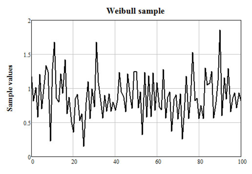
as the unknown true functions to be estimated. Parameters of the densities are selected to satisfy the integrated conditions of the Theorem above. We generated Maxwell and Weibull samples with sample length using standard generators (see Fig. 2).
Based on these samples and the method of moments (12), we obtain the parameter values and for the reference gamma density (11). Substitution of it into the expression (8) for the optimal bandwidth leads to the estimate by the rule of thumb
| (16) |
Similar computations were performed for the sample from a Maxwell distribution. C
Density derivative estimates corresponding to calculated bandwidths are represented on Fig. 3 and Fig. 4. Here solid line corresponds to the true density derivative to be estimated, dashed line corresponds to rule of thumb estimates.


Quantitatively, the estimation error is determined by the value , defined by the following formula:
| (17) |
The mean error
calculated over repeated experiments and standard deviations in brackets are represented in Table 3 and Table 4.
| m | rule of thumb |
|---|---|
| 0.0082 | |
| 0.02302 | |
| 0.015314 |
| m | rule of thumb |
|---|---|
| 0.61945 | |
| 0.25808 | |
| 0.17994 |
From the tables and graphics one can see that from two methods of bandwidth selection (the rule of thumb and cross-validation) better results gives the latter one.
5 CONCLUSIONS
Estimation of the probability characteristics of the positive random variables is required in the theory of signal processing, the financial and actuarial mathematics and other important applications. The positivity of the distribution support of the observed random variables results in a significant complication of the models compared to the case of an unbounded support. We present nonparametric kernel estimates of the densities and their derivatives based on the asymmetric gamma kernels. The main part of the paper is devoted to the construction and evaluation of the optimal smoothing parameters (bandwidths) in the kernel density derivative estimates by samples of the independent random variables. For this purpose two well-known method such as the rule of thumb is used. It should be noted that in the case of asymmetric support even for the simple rule of thumb method the expression for the smoothing parameter (15) becomes quite cumbersome in comparison with the known corresponding expression based on the Gaussian reference function defined on the whole line. The estimates of the kernel density derivatives will be used for the nonparametric estimation of logarithmic derivatives of the density determined on the positive real axis. The latter can be used for the problems of unsupervised nonparametric signal processing.