跳到论文正文
W Papers独立论文阅读器 arXiv:1401.6664 论文正文 计算阅读时间 · 0%
引用这篇论文根据当前论文元数据生成,正式投稿前建议核对。


License: arXiv.org perpetual non-exclusive license
arXiv:1401.6664v3 [math.DS] 25 Jun 2014

A new concept of local metric entropy for
finite-time nonautonomous dynamical systems

Luu Hoang Duc Affiliation: Institute of Mathematics, VAST, Vietnam & Affiliation: Center for Dynamics, Technische Universität Dresden Affiliation: lhduc@math.ac.vn, hoang_duc.luu@tu-dresden.de Affiliation: Stefan Siegmund Affiliation: Institute for Analysis & Center for Dynamics Affiliation: Technische Universität Dresden Email: stefan.siegmund@tu-dresden.de
Abstract

We introduce a new concept of finite-time entropy which is a local version of the classical concept of metric entropy. Based on that, a finite-time version of Pesin’s entropy formula and also an explicit formula of finite-time entropy for 22-D systems are derived. We also discuss about how to apply the finite-time entropy field to detect special dynamical behavior such as Lagrangian coherent structures.

Key words and phrases: finite-time metric entropy (FTME), finite-time Lyapunov exponents (FTLE), Pesin’s formula, Lagrangian coherent structures (LCS)
2010 Mathematics Subject Classification: 54C70; 28D20; 37A35; 37M25; 37D25

1 Introduction

Metric or measure-theoretic entropy for a transformation was introduced by Kolmogorov and Sinai in 1959; the ideas go back to Shannon’s information theory (see Young [26] for a well-written survey and the references therein). Concepts and results on metric entropy can be formulated in general settings [26]. We recall some basic facts for the special situation of a map T:M→MT:M\rightarrow M on a compact set M⊂ℝnM\subset\mathbb{R}^{n} which is measure-preserving w.r.t. the Lebesgue measure μ\mu, i.e. for every Borel set AA, T−1​AT^{-1}A is also a Borel set, and μ⁡(A)=μ⁡(T−1​A)\mu(A)=\mu(T^{-1}A). The metric entropy hμ​(T)h_{\mu}(T) of TT w.r.t. μ\mu can be defined as the supremum over all entropies of finite partitions of MM. However, we are particularly interested in a local characterization of metric entropy which goes back to Bowen [3, Definition 6 & Proposition 7] (see also [4, 26]) and was then generalized by Thieullen [23, 24]. According to Thieullen [23], for any x∈Mx\in M, n∈ℕ,α≥0n\in\mathbb{N},\alpha\geq 0 and ε>0\varepsilon>0, define

Bα​(x,n,ε):={y∈X:sup0≤i≤n‖Ti​x−Ti​y‖​ei​α<ε}B^{\alpha}(x,n,\varepsilon):=\{y\in X:\sup_{0\leq i\leq n}\|T^{i}x-T^{i}y\|e^{i\alpha}<\varepsilon\} (1)

and the local quantities

h¯μ​(α,T,x):⁣=limε→0lim supn→∞−1nlogμ(Bα(x,n,ε)),h¯μ​(α,T,x):⁣=limε→0lim infn→∞−1nlogμ(Bα(x,n,ε)).\begin{array}[]{rcl}\overline{h}_{\mu}(\alpha,T,x)&:=&\lim_{\varepsilon\to 0}\limsup_{n\to\infty}-\frac{1}{n}\log\mu\big(B^{\alpha}(x,n,\varepsilon)\big),\\[4.30554pt] \underline{h}_{\mu}(\alpha,T,x)&:=&\lim_{\varepsilon\to 0}\liminf_{n\to\infty}-\frac{1}{n}\log\mu\big(B^{\alpha}(x,n,\varepsilon)\big).\end{array} (2)

If TT is a C2C^{2} diffeomorphism then h¯μ​(α,T,x)=h¯μ​(α,T,x)=:hμ​(α,T,x)\overline{h}_{\mu}(\alpha,T,x)=\underline{h}_{\mu}(\alpha,T,x)=:h_{\mu}(\alpha,T,x) and we call hμh_{\mu} the local α\alpha-entropy. Moreover, if α=0\alpha=0 and TT is ergodic then hμ​(α,T,x)=hμ​(T)h_{\mu}(\alpha,T,x)=h_{\mu}(T) for almost every x∈Mx\in M [4]. Local α\alpha-entropy also has the interpretation of being the rate of loss of information on nearby orbits. Its relation to the Lyapunov exponents of TT are described by Pesin’s formula [18, 19, 23]. Let λn​(x)≤…≤λ1​(x)\lambda_{n}(x)\leq\ldots\leq\lambda_{1}(x) denote the Lyapunov exponents of TT at the point xx. Write a+=max⁡(a,0)a^{+}=\max(a,0).

Theorem 1 (Pesin’s formula for α\alpha-entropy [23]).

Let T:M→MT:M\to M be a C2C^{2} diffeomorphism preserving the Lebesgue measure μ\mu. Then for almost every x∈Mx\in M

hμ​(α,T,x)={∑i=1n(λi​(x)+α)+if​ 0≤α≤−λn​(x),n​αif​α≥−λn​(x).h_{\mu}(\alpha,T,x)=\left\{\begin{array}[]{ll}\sum_{i=1}^{n}(\lambda_{i}(x)+\alpha)^{+}&\text{if}\ 0\leq\alpha\leq-\lambda_{n}(x)\,,\\[4.30554pt] n\alpha&\text{if}\ \alpha\geq-\lambda_{n}(x)\,.\end{array}\right.

In Section 2 we introduce a new concept of finite-time metric entropy (FTME) which is motivated by the local quantities (2). The notion of FTME is defined in Definition 5 w.r.t. the Lebesgue measure in the setting of nonautonomous dynamical systems (NDS) on fibre bundles X⊆ℝn×JX\subseteq\mathbb{R}^{n}\times J over compact subsets JJ of ℝ\mathbb{R} and can be easily adapted to NDS on Riemannian manifolds with measures which are equivalent to the Riemannian measure. Our concept of FTME is related to, but formally different from the probabilistic concept of finite-time entropy (FTE) introduced by Froyland and Padberg-Gehle [8] which is based on the concept of differential entropy for a smoothed transfer operator (see Remark 6(e) for a comparison). FTME of a nonlinear NDS can be expressed by FTME of its linearization (Theorem 8) and is proportional to the measure of the intersection of ellipsoids which are the preimages of balls under the linearized NDS (Corollary 10).

In Section 3 we prove a finite-time version of Pesin’s formula from Theorem 1 which relates the FTME to the sum of finite-time Lyapunov exponents which are not less than the weight factor α\alpha. For one and two-dimensional NDS an exact formula is given in (23) and Proposition 13. The main approximation result which holds in arbitrary dimensions is contained in Theorem 16.

In Section 4 we introduce Lagrangian coherent structures (LCS) based on the new notion of FTME. For a discussion of LCS based on finite-time Lyapunov exponents see e.g. [11, 12] and the references therein. In order to formulate Theorem 2 in [12] for two-dimensional differential equations (see also [11, 12] for arbitrary dimensions), consider a planar differential equation x˙=f⁡(t,x)\dot{x}=f(t,x), t∈[t0,t0+T]t\in[t_{0},t_{0}+T], x∈ℝ2x\in\mathbb{R}^{2}, for some T>0T>0 with solution φ⁡(t,s)​x0\varphi(t,s)x_{0} which takes the initial value x0x_{0} at t=st=s. Let Λ1​(t0,x0,T)≥Λ2​(t0,x0,T)\Lambda_{1}(t_{0},x_{0},T)\geq\Lambda_{2}(t_{0},x_{0},T) and ξ1​(t0,x0,T),ξ2​(t0,x0,T)\xi_{1}(t_{0},x_{0},T),\xi_{2}(t_{0},x_{0},T) denote the singular values and singular vectors of Φx0​(t0+T,t0):=D​φ​(t0+T,t0)​x0\Phi_{x_{0}}(t_{0}+T,t_{0}):=D\varphi(t_{0}+T,t_{0})x_{0}, respectively, i.e. Φx0​(t0+T,t0)⊤​Φx0​(t0+T,t0)​ξi​(t0,x0,T)=Λi​(t0,x0,T)​ξi​(t0,x0,T)\Phi_{x_{0}}(t_{0}+T,t_{0})^{\top}\Phi_{x_{0}}(t_{0}+T,t_{0})\xi_{i}(t_{0},x_{0},T)=\Lambda_{i}(t_{0},x_{0},T)\xi_{i}(t_{0},x_{0},T). The finite-time Lyapunov exponents (FTLE) are defined by λi​(t0,x0,T):=1T​log⁡Λi​(t0,x0,T)\lambda_{i}(t_{0},x_{0},T):=\frac{1}{T}\log\Lambda_{i}(t_{0},x_{0},T). Note that λ1​(t0,x0,T)≥λ2​(t0,x0,T)\lambda_{1}(t_{0},x_{0},T)\geq\lambda_{2}(t_{0},x_{0},T) (in contrast to the reversed order in [12]). Consider a smooth compact curve ℳ⁡(t)⊂ℝ2\mathcal{M}(t)\subset\mathbb{R}^{2} at time t0t_{0} which is mapped by the solution map into a time-evolving curve ℳ⁡(t)=φ⁡(t,t0)​ℳ​(t0)\mathcal{M}(t)=\varphi(t,t_{0})\mathcal{M}(t_{0}). For each x0∈ℳ⁡(t0)x_{0}\in\mathcal{M}(t_{0}) denote the tangent space of ℳ⁡(t0)\mathcal{M}(t_{0}) at x0x_{0} by Tx0​ℳ​(t0)T_{x_{0}}\mathcal{M}(t_{0}).

Theorem 2 (LCS and Weak LCS in Two Dimensions [12, Thm. 2]).

(i) ℳ⁡(t)\mathcal{M}(t) is a repelling weak LCS (WLCS) over [t0,t0+T][t_{0},t_{0}+T] if and only for all x0∈ℳ⁡(t0)x_{0}\in\mathcal{M}(t_{0}):

  • 1.

    Λ2​(t0,x0,T)≠Λ1​(t0,x0,T)>1\Lambda_{2}(t_{0},x_{0},T)\neq\Lambda_{1}(t_{0},x_{0},T)>1

  • 2.

    ξ1​(t0,x0,T)⟂Tx0​ℳ​(t0)\xi_{1}(t_{0},x_{0},T)\perp T_{x_{0}}\mathcal{M}(t_{0})

  • 3.

    ⟨∇Λ1​(t0,x0,T),ξ1​(t0,x0,T)⟩=0\langle\nabla\Lambda_{1}(t_{0},x_{0},T),\xi_{1}(t_{0},x_{0},T)\rangle=0

(ii) ℳ⁡(t)\mathcal{M}(t) is a repelling LCS over [t0,t0+T][t_{0},t_{0}+T] if and only if:

  • 1.

    ℳ⁡(t)\mathcal{M}(t) is a repelling WLCS over [t0,t0+T][t_{0},t_{0}+T]

  • 2.

    ⟨ξ1​(t0,x0,T),∇2Λ1​(t0,x0,T)​ξ1​(t0,x0,T)⟩<0\langle\xi_{1}(t_{0},x_{0},T),\nabla^{2}\Lambda_{1}(t_{0},x_{0},T)\xi_{1}(t_{0},x_{0},T)\rangle<0

In constrast to emphasizing the normal direction of ℳ\mathcal{M} in condition 2 of Theorem 2(i), we introduce a stretching rate along the direction of the vector field in Section 4 and use this as a (local in time and space) weight factor for normalizing the exponential growth rates. This weight factor leads to a loss of frame-independence (cp. Remark 21), but is chosen adequately so that we can show in Theorem 20 and explicitely for a family of nonlinear autonomous equations in Example 17 and even for linear systems in Example 18, that the ridge and trough-like structures of this weighted FTME field are able to recover stable and unstable manifolds. See also [5, 6] for alternative approaches to finite-time spectrum and hyperbolicity.

2 Finite-time entropy

Let J⊆ℝJ\subseteq\mathbb{R} and (X⁡(t))t∈J⊆ℝn\big(X(t)\big)_{t\in J}\subseteq\mathbb{R}^{n} be a family of subsets of ℝn\mathbb{R}^{n} indexed by JJ. Then X:={(t,x)∈J×ℝn:x∈X⁡(t)}X:=\{(t,x)\in J\times\mathbb{R}^{n}:x\in X(t)\} is a (trivial) fibre bundle over the base space JJ.

A continuous map φ:J×X→X\varphi:J\times X\rightarrow X is called a nonautonomous dynamical system (NDS) on XX over JJ, if for t,u,s∈Jt,u,s\in J and x∈X⁡(s)x\in X(s) the properties φ⁡(s,s,x)=(s,x)\varphi(s,s,x)=(s,x) and φ⁡(t,u,φ⁡(u,s,x))=(t,φ⁡(t,s,x))\varphi(t,u,\varphi(u,s,x))=(t,\varphi(t,s,x)) hold. For ease of notation we identify φ\varphi with the two-parameter family of maps φ(t,s)=φ(t,s,⋅):X(s)→X(t)⊆ℝn\varphi(t,s)=\varphi(t,s,\cdot):X(s)\rightarrow X(t)\subseteq\mathbb{R}^{n}, t,s∈Jt,s\in J, and the defining properties read as

φ⁡(s,s)​x=xandφ⁡(t,u)∘φ⁡(u,s)​x=φ⁡(t,s)​x.\varphi(s,s)x=x\quad\text{and}\quad\varphi(t,u)\circ\varphi(u,s)x=\varphi(t,s)x.

Obviously φ​(t,s)−1=φ⁡(s,t)\varphi(t,s)^{-1}=\varphi(s,t). If JJ is compact, then φ\varphi is called finite-time nonautonomous dynamical system (FTNDS). If for all t,s∈Jt,s\in J the maps φ⁡(t,s):X⁡(t)→X⁡(s)\varphi(t,s):X(t)\to X(s) are CkC^{k} and all derivatives depend continuously on t,s∈Jt,s\in J, we say that φ\varphi is CkC^{k}. We write |J|:=max⁡J−min⁡J|J|:=\max{J}-\min{J}.

Note that the term nonautonomous dynamical system (NDS) is sometimes used in slightly different contexts (see e.g. [2] and the references therein), either refering to a cocycle (with time tt measuring the time which elapsed since the starting time) or a process (with time tt measuring absolute time).

Example 3.

(a) A homeomorphism T:M→MT:M\rightarrow M on M⊆ℝnM\subseteq\mathbb{R}^{n} generates an NDS φ⁡(t,s)​x:=Tt−s​x\varphi(t,s)x:=T^{t-s}x on ℤ×M\mathbb{Z}\times M over ℤ\mathbb{Z}.

(b) Let D⊆ℝ×ℝnD\subseteq\mathbb{R}\times\mathbb{R}^{n} be open and f∈Ck​(D,ℝn)f\in C^{k}(D,\mathbb{R}^{n}) for some k∈ℕk\in\mathbb{N}. For (t0,x0)∈D(t_{0},x_{0})\in D let φ⁡(⋅,t0,x0)\varphi(\cdot,t_{0},x_{0}) denote the solution of the initial value problem

x˙=f⁡(t,x),x⁡(t0)=x0.\dot{x}=f(t,x),\quad x(t_{0})=x_{0}.

If for an arbitrary J⊆ℝJ\subseteq\mathbb{R} and a family (X⁡(t))t∈J\big(X(t)\big)_{t\in J} of subsets of ℝn\mathbb{R}^{n} each map φ(t,s,⋅):X(s)→X(t)\varphi(t,s,\cdot):X(s)\rightarrow X(t), for t,s∈Jt,s\in J, is well-defined, then φ\varphi is an NDS on XX over JJ and is CkC^{k}.

(c) In the setting of (b), let Φx0​(t,s)\Phi_{x_{0}}(t,s) denote the solution matrix of the linearization v˙=Dx​f​(t,φ⁡(t,s,x0))​v\dot{v}=D_{x}f(t,\varphi(t,s,x_{0}))v which satisfies Φx0​(s,s)=In×n\Phi_{x_{0}}(s,s)=I_{n\times n} for (s,x0)∈X(s,x_{0})\in X, t∈Jt\in J. Then D​φ​(t,s)​x0=Φx0​(t,s)D\varphi(t,s)x_{0}=\Phi_{x_{0}}(t,s) and Φx0\Phi_{x_{0}} is a linear NDS on XX over JJ.

Let ∥⋅∥\|\cdot\| denote the Euclidean norm on ℝn\mathbb{R}^{n}. For a finite-time NDS φ\varphi on XX over a compact JJ we want to measure the distance of orbits 𝒪⁡(t0,x):={(t,φ⁡(t,t0)​x):t∈J}⊂X{\cal O}(t_{0},x):=\big\{\big(t,\varphi(t,t_{0})x\big):t\in J\big\}\subset X to other orbits 𝒪⁡(t0,y){\cal O}(t_{0},y) and thereto introduce a parametrized family dα:X×JX→J×ℝ0+d^{\alpha}:X\times_{J}X\rightarrow J\times\mathbb{R}_{0}^{+}, (t0,x,y)↦(t0,dt0α​(x,y))(t_{0},x,y)\mapsto(t_{0},d_{t_{0}}^{\alpha}(x,y)), of fibre metrics on the fibre product X×JX:=((X⁡(t)×X⁡(t))t∈JCLOSEX\times_{J}X:=\big((X(t)\times X(t)\big)_{t\in J}, by defining for α∈ℝ\alpha\in\mathbb{R} the weighted orbit metric

dt0α​(x,y):=supt∈J‖φ⁡(t,t0)​y−φ⁡(t,t0)​x‖​e−α⁡(t−t0).d_{t_{0}}^{\alpha}(x,y):=\sup_{t\in J}\|\varphi(t,t_{0})y-\varphi(t,t_{0})x\|e^{-\alpha(t-t_{0})}. (3)

The dependency of dt0α=dt0φ,J,αd_{t_{0}}^{\alpha}=d_{t_{0}}^{\varphi,J,\alpha} on φ\varphi and JJ is sometimes denoted in the superscript. Using the fact that (t,x)∈𝒪⁡(t0,x0)⇔x=φ⁡(t,t0)​x0(t,x)\in{\cal O}(t_{0},x_{0})\Leftrightarrow x=\varphi(t,t_{0})x_{0}, it is easy to see that

dt0α(x0,y0)≤ε⇔∀(t,x)∈𝒪(t0,x0),(t,y)∈𝒪(t0,y0):∥x−y∥≤εe−α​t0⋅eα​t.d_{t_{0}}^{\alpha}(x_{0},y_{0})\leq\varepsilon\quad\Leftrightarrow\quad\forall(t,x)\in{\cal O}(t_{0},x_{0}),(t,y)\in{\cal O}(t_{0},y_{0}):\|x-y\|\leq\varepsilon e^{-\alpha t_{0}}\cdot e^{\alpha t}.

The balls w.r.t. the orbit metric are denoted by

Bt0α​(x0,ε):={x∈X⁡(t0):dt0α​(x,x0)≤ε}for ​(t0,x0)∈X,ε≥0.B_{t_{0}}^{\alpha}(x_{0},\varepsilon):=\{x\in X(t_{0}):d_{t_{0}}^{\alpha}(x,x_{0})\leq\varepsilon\}\qquad\text{for }(t_{0},x_{0})\in X,\varepsilon\geq 0.

Since dt0α​(x,x0)≤‖x−x0‖d_{t_{0}}^{\alpha}(x,x_{0})\leq\|x-x_{0}\|, obviously Bt0α​(x0,ε)⊆B⁡(x0,ε):={x∈ℝn:‖x−x0‖≤ε}B_{t_{0}}^{\alpha}(x_{0},\varepsilon)\subseteq B(x_{0},\varepsilon):=\{x\in\mathbb{R}^{n}:\|x-x_{0}\|\leq\varepsilon\}.

Proposition 4 (Properties of orbit metric).

Let φ\varphi be an FTNDS on XX over JJ.

(i) Invariance: For (t0,x0)∈X,ε≥0(t_{0},x_{0})\in X,\varepsilon\geq 0 and arbitrary t∈Jt\in J

φ⁡(t,t0)​Bt0α​(x0,ε)=Btα​(φ⁡(t,t0)​x0,ε​eα⁡(t−t0)).\varphi(t,t_{0})B_{t_{0}}^{\alpha}(x_{0},\varepsilon)=B_{t}^{\alpha}\big(\varphi(t,t_{0})x_{0},\varepsilon e^{\alpha(t-t_{0})}\big). (4)

(ii) Monotonicity: For (t0,x0)∈X(t_{0},x_{0})\in X, 0≤ε1≤ε20\leq\varepsilon_{1}\leq\varepsilon_{2} and t0∈J2⊆J1⊆Jt_{0}\in J_{2}\subseteq J_{1}\subseteq J

Bt0J1,α​(x0,ε1)⊆Bt0J2,α​(x0,ε2).B_{t_{0}}^{J_{1},\alpha}(x_{0},\varepsilon_{1})\subseteq B_{t_{0}}^{J_{2},\alpha}(x_{0},\varepsilon_{2}). (5)
Proof.

(i) We rewrite Bt0α​(x0,ε)B_{t_{0}}^{\alpha}(x_{0},\varepsilon) in the following form

Bt0α​(x0,ε)\displaystyle B_{t_{0}}^{\alpha}(x_{0},\varepsilon) =\displaystyle= {x∈X⁡(t0):‖φ⁡(t,t0)​x−φ⁡(t,t0)​x0‖≤ε​eα⁡(t−t0)​∀t∈J}\displaystyle\big\{x\in X(t_{0}):\|\varphi(t,t_{0})x-\varphi(t,t_{0})x_{0}\|\leq\varepsilon e^{\alpha(t-t_{0})}\;\forall t\in J\big\} (6)
=\displaystyle= {x∈X⁡(t0):φ⁡(t,t0)​x∈B⁡(φ⁡(t,t0)​x0,ε​eα⁡(t−t0))​∀t∈J}\displaystyle\big\{x\in X(t_{0}):\varphi(t,t_{0})x\in B\big(\varphi(t,t_{0})x_{0},\varepsilon e^{\alpha(t-t_{0})}\big)\;\forall t\in J\big\}
=\displaystyle= {x∈X⁡(t0):x∈φ​(t,t0)−1​B​(φ⁡(t,t0)​x0,ε​eα⁡(t−t0))​∀t∈J}\displaystyle\big\{x\in X(t_{0}):x\in\varphi(t,t_{0})^{-1}B\big(\varphi(t,t_{0})x_{0},\varepsilon e^{\alpha(t-t_{0})}\big)\;\forall t\in J\big\}
=\displaystyle= ⋂t∈Jφ​(t,t0)−1​B​(φ⁡(t,t0)​x0,ε​eα⁡(t−t0)).\displaystyle\bigcap_{t\in J}\varphi(t,t_{0})^{-1}B\big(\varphi(t,t_{0})x_{0},\varepsilon e^{\alpha(t-t_{0})}\big).

To derive (4), we observe that for t∈Jt\in J

φ⁡(t,t0)​Bt0α​(x0,ε)\displaystyle\varphi(t,t_{0})B_{t_{0}}^{\alpha}(x_{0},\varepsilon) =\displaystyle= φ⁡(t,t0)​⋂s∈Jφ​(s,t0)−1​B​(φ⁡(s,t0)​x0,ε​eα⁡(s−t0))\displaystyle\varphi(t,t_{0})\bigcap_{s\in J}\varphi(s,t_{0})^{-1}B\big(\varphi(s,t_{0})x_{0},\varepsilon e^{\alpha(s-t_{0})}\big)
=\displaystyle= ⋂s∈Jφ⁡(t,t0)​φ​(s,t0)−1​B​(φ⁡(s,t0)​x0,ε​eα⁡(s−t0))\displaystyle\bigcap_{s\in J}\varphi(t,t_{0})\varphi(s,t_{0})^{-1}B\big(\varphi(s,t_{0})x_{0},\varepsilon e^{\alpha(s-t_{0})}\big)
=\displaystyle= ⋂s∈Jφ​(s,t)−1​B​(φ⁡(s,t)​φ​(t,t0)​x0,ε​eα⁡(t−t0)​eα⁡(s−t))\displaystyle\bigcap_{s\in J}\varphi(s,t)^{-1}B\big(\varphi(s,t)\varphi(t,t_{0})x_{0},\varepsilon e^{\alpha(t-t_{0})}e^{\alpha(s-t)}\big)
=\displaystyle= Btα​(φ⁡(t,t0)​x0,ε​eα⁡(t−t0)).\displaystyle B_{t}^{\alpha}(\varphi(t,t_{0})x_{0},\varepsilon e^{\alpha(t-t_{0})}).

(ii) If ε1≤ε2\varepsilon_{1}\leq\varepsilon_{2} and J2⊆J1J_{2}\subseteq J_{1} then dt0J2,α​(x,y)≤dt0J1,α​(x,y)d_{t_{0}}^{J_{2},\alpha}(x,y)\leq d_{t_{0}}^{J_{1},\alpha}(x,y) for x,y∈X⁡(t0)x,y\in X(t_{0}) and the claim follows. ∎

Definition 5 (Finite-time metric entropy (FTME)).

Let φ\varphi be an FTNDS on XX over JJ and α∈ℝ\alpha\in\mathbb{R}. The finite-time metric entropy (FTME) with weight α\alpha at (t0,x0)∈X(t_{0},x_{0})\in X is defined by

ht0α​(x0):=lim supε→0ht0α​(x0,ε)with ​ht0α​(x0,ε):=−1|J|​log⁡μ⁡(Bt0α​(x0,ε))μ⁡(B⁡(x0,ε)).h_{t_{0}}^{\alpha}(x_{0}):=\limsup_{\varepsilon\to 0}h_{t_{0}}^{\alpha}(x_{0},\varepsilon)\qquad\text{with }h_{t_{0}}^{\alpha}(x_{0},\varepsilon):=-\frac{1}{|J|}\log\frac{\mu\big(B_{t_{0}}^{\alpha}(x_{0},\varepsilon)\big)}{\mu\big(B(x_{0},\varepsilon)\big)}. (7)

The dependency of ht0α=ht0φ,J,αh_{t_{0}}^{\alpha}=h_{t_{0}}^{\varphi,J,\alpha} on φ\varphi and JJ is sometimes denoted in the superscript.

Remark 6 (Finite-time escape rate).

(a) Definition 5 can be seen as a finite-time version of the local α\alpha-entropy introduced by Thieullen [23] to FTNDS which are not necessarily measure-preserving. However, in contrast to [23], we will study FTME for weight factors α\alpha which might depend on x0x_{0} and are not just a constant. We will exploit this idea in Section 4 in Theorem 20 to construct new candidates of Lagrangian coherent structures.

(b) The quantity ht0α​(x0,ε)h_{t_{0}}^{\alpha}(x_{0},\varepsilon) in (7) is called finite-time α\alpha-escape rate of radius ε>0\varepsilon>0 at (t0,x0)(t_{0},x_{0}). It measures how many points escape from the ε\varepsilon-orbit neighborhood of the orbit 𝒪⁡(t0,x0){\cal O}(t_{0},x_{0}) on JJ, since with the first-order approximation log⁡x≈x−1\log x\approx x-1 for x≈1x\approx 1, and using the fact that Bt0α​(x0,ε)⊂B⁡(x0,ε)B_{t_{0}}^{\alpha}(x_{0},\varepsilon)\subset B(x_{0},\varepsilon), we have

ht0α​(x0,ε)≈1|J|​[1−μ⁡(Bt0α​(x0,ε))μ⁡(B⁡(x0,ε))]=1|J|​μ⁡(B⁡(x0,ε)∖Bt0α​(x0,ε))μ⁡(B⁡(x0,ε))h_{t_{0}}^{\alpha}(x_{0},\varepsilon)\approx\frac{1}{|J|}\bigg[1-\frac{\mu\big(B_{t_{0}}^{\alpha}(x_{0},\varepsilon)\big)}{\mu\big(B(x_{0},\varepsilon)\big)}\bigg]=\frac{1}{|J|}\frac{\mu\big(B(x_{0},\varepsilon)\setminus B_{t_{0}}^{\alpha}(x_{0},\varepsilon)\big)}{\mu\big(B(x_{0},\varepsilon)\big)}

if μ⁡(Bt0α​(x0,ε))μ⁡(B⁡(x0,ε))≈1\frac{\mu(B_{t_{0}}^{\alpha}(x_{0},\varepsilon))}{\mu(B(x_{0},\varepsilon))}\approx 1.

(c) Let φ\varphi be an NDS on ℤ×M\mathbb{Z}\times M over ℤ\mathbb{Z} generated by a homeomorphism T:M→MT:M\rightarrow M as in Example 3(a). In order to relate the metric entropy hμ​(T,x)h_{\mu}(T,x) of TT at xx to the FTME, more precisely, to the finite-time escape rate, define the sets Jn:={0,1,…,n}J_{n}:=\{0,1,\dots,n\} for n∈ℕn\in\mathbb{N}. Using the fact that |Jn|=n|J_{n}|=n and B⁡(x,n,ε)B(x,n,\varepsilon) in (1) equals Bt0Jn,α​(x,ε)B_{t_{0}}^{J_{n},\alpha}(x,\varepsilon) for t0=0t_{0}=0 and α=0\alpha=0, we get lim supn→∞h0Jn,0(x,ε)=lim supn→∞−1n(logB0Jn,0(x,ε)−logB(x,ε))\limsup_{n\to\infty}h_{0}^{J_{n},0}(x,\varepsilon)=\limsup_{n\to\infty}-\frac{1}{n}(\log B_{0}^{J_{n},0}(x,\varepsilon)-\log B(x,\varepsilon)) and hence

hμ​(T,x)=lim supε→0lim supn→∞h0Jn,0​(x,ε).h_{\mu}(T,x)=\limsup_{\varepsilon\to 0}\limsup_{n\to\infty}h_{0}^{J_{n},0}(x,\varepsilon).

(d) If φ\varphi is an NDS on XX over a two-point set J={t0,t0+T}J=\{t_{0},t_{0}+T\} for some t0∈ℝt_{0}\in\mathbb{R} and T>0T>0, then (6) for α=0\alpha=0 implies Bt00​(x0,ε)=B⁡(x0,ε)∩φ​(t0+T,t0)−1​B​(φ⁡(t0+T,t0)​x0,ε)B_{t_{0}}^{0}(x_{0},\varepsilon)=B(x_{0},\varepsilon)\cap\varphi(t_{0}+T,t_{0})^{-1}B(\varphi(t_{0}+T,t_{0})x_{0},\varepsilon), and with (7) we get for the finite-time escape rate ht00​(x0,ε)h_{t_{0}}^{0}(x_{0},\varepsilon) the relation

μ⁡(φ​(t0+T,t0)−1​B​(φ⁡(t0+T,t0)​x0,ε)∩B⁡(x0,ε))μ⁡(B⁡(x0,ε))=e−ht00​(x0,ε)​T.\frac{\mu\big(\varphi(t_{0}+T,t_{0})^{-1}B(\varphi(t_{0}+T,t_{0})x_{0},\varepsilon)\cap B(x_{0},\varepsilon)\big)}{\mu(B(x_{0},\varepsilon))}=e^{-h_{t_{0}}^{0}(x_{0},\varepsilon)T}. (8)

If ht00​(x0,ε)≈0h_{t_{0}}^{0}(x_{0},\varepsilon)\approx 0 then the pair of sets At0:=B⁡(x0,ε)A_{t_{0}}:=B(x_{0},\varepsilon), At0+T:=B⁡(φ⁡(t0+T,t0)​x0,ε)A_{t_{0}+T}:=B(\varphi(t_{0}+T,t_{0})x_{0},\varepsilon), satisfies At0≈φ​(t0+T,t0)−1​At0+TA_{t_{0}}\approx\varphi(t_{0}+T,t_{0})^{-1}A_{t_{0}+T} and is called pair of coherent sets in [9, 10]. In other words, the FTME ht00​(x0)h_{t_{0}}^{0}(x_{0}) over a two-point set {t0,t0+T}\{t_{0},t_{0}+T\} is an average logarithmic measure of coherence of infinitesimally small balls centered at x0x_{0} and φ⁡(t0+T,t0)​x0\varphi(t_{0}+T,t_{0})x_{0}.

(e) Finite-time metric entropy (FTME) in Definition 5 and finite-time entropy (FTE) [8, Definition 4.1] can be expressed in terms of differential entropy which is defined by hdiff(f)=−∫ℝnf(x)logf(x)dμ(x)h_{\operatorname{diff}}(f)=-\int_{\mathbb{R}^{n}}f(x)\log f(x)\,d\mu(x) for f∈L1​(ℝn)f\in L^{1}(\mathbb{R}^{n}) and goes back to Boltzmann (see [16, Chapter 9] for a discussion in the dynamical systems context). FTE for an NDS φ\varphi on XX over a two-point time set J={t0,t0+T}J=\{t_{0},t_{0}+T\} satisfies

F​T​E​(x0,t0,T)=limε→01|T|​[hdiff​(𝒜ε​𝒫t0,T​fB⁡(x0,ε))−hdiff​(fB⁡(x0,ε))]with ​fA:=1μ⁡(A)​𝟙A​(⋅)FTE(x_{0},t_{0},T)=\lim_{\varepsilon\to 0}\frac{1}{|T|}\big[h_{\operatorname{diff}}(\mathcal{A}_{\varepsilon}\mathcal{P}_{t_{0},T}f_{B(x_{0},\varepsilon)})-h_{\operatorname{diff}}(f_{B(x_{0},\varepsilon)})\big]\quad\text{with }f_{A}:=\frac{1}{\mu(A)}\mathds{1}_{A}(\cdot)

and compares the differential entropy of a scaled characteristic function on an ε\varepsilon-ball with a push-forward of that function by the Perron-Frobenius operator 𝒫t0,T​f​(x)=f⁡(φ​(t0+T,t0)−1​x)|detDx​φ​(t0+T,t0)​φ​(t0+T,t0)−1​x|\mathcal{P}_{t_{0},T}f(x)=\frac{f(\varphi(t_{0}+T,t_{0})^{-1}x)}{|\det D_{x}\varphi(t_{0}+T,t_{0})\varphi(t_{0}+T,t_{0})^{-1}x|} followed by an ε\varepsilon-smoothing 𝒜ε​f​(x)=1μ⁡(B⁡(x,ε))​∫B⁡(x,ε)f​𝑑μ\mathcal{A}_{\varepsilon}f(x)=\frac{1}{\mu(B(x,\varepsilon))}\int_{B(x,\varepsilon)}f\,d\mu.

FTME for an NDS φ\varphi on XX over a compact time set J⊂ℝJ\subset\mathbb{R} for some t0∈Jt_{0}\in J and weight factor α∈ℝ\alpha\in\mathbb{R} is

ht0α​(x0)=limε→01|J|​[hdiff​(fBt0α​(x0,ε))−hdiff​(fB⁡(x0,ε))].h_{t_{0}}^{\alpha}(x_{0})=\lim\limits_{\varepsilon\to 0}\frac{1}{|J|}\big[h_{\operatorname{diff}}(f_{B_{t_{0}}^{\alpha}(x_{0},\varepsilon)})-h_{\operatorname{diff}}(f_{B(x_{0},\varepsilon)})\big].

The comparison of FTME and FTE will be the subject of further studies. To illustrate one possible relation between FTE and FTME, let φ\varphi be an NDS on XX over a two-point time set J={t0,t0+T}J=\{t_{0},t_{0}+T\}. Assume for simplicity that X⁡(t0)=X⁡(t0+T)X(t_{0})=X(t_{0}+T) and let ℬ={B1,…,Bn}{\cal B}=\{B_{1},\dots,B_{n}\} be a partition of the state space X⁡(t0)=X⁡(t0+T)X(t_{0})=X(t_{0}+T). Then formula (8) suggests that the FTME ht00​(x0)h_{t_{0}}^{0}(x_{0}) could be approximated by

−1T​log⁡μ⁡(φ​(t0+T,t0)−1​Bj∩Bi)μ⁡(Bi)-\frac{1}{T}\log\frac{\mu(\varphi(t_{0}+T,t_{0})^{-1}B_{j}\cap B_{i})}{\mu(B_{i})}

where x0∈Bix_{0}\in B_{i} and φ⁡(t0+T,t0)​x0∈Bj\varphi(t_{0}+T,t_{0})x_{0}\in B_{j} for some i,ji,j. On the other hand, F​T​E​(x0,t0,T)FTE(x_{0},t_{0},T), with x0∈Bix_{0}\in B_{i} for some ii, is approximated by a localized version of the Kolmogorov-Shannon entropy

−1T∑j=1nμ⁡(Bi∩φ​(t0+T,t0)−1​Bj)μ⁡(Bi)logμ⁡(Bi∩φ​(t0+T,t0)−1​Bj)μ⁡(Bi)-\frac{1}{T}\sum_{j=1}^{n}\frac{\mu(B_{i}\cap\varphi(t_{0}+T,t_{0})^{-1}B_{j})}{\mu(B_{i})}\log\frac{\mu(B_{i}\cap\varphi(t_{0}+T,t_{0})^{-1}B_{j})}{\mu(B_{i})}

of the partition ℬ\cal B.

The following proposition states that FTME is constant for linear nonautonomous dynamical systems. A similar statement for FTE can be found in [8, Lemma 2.6]. Note, however, that the FTME with an exponential weight factor α=α⁡(x0)\alpha=\alpha(x_{0}) which depends on x0∈X⁡(t0)x_{0}\in X(t_{0}) for some t0∈Jt_{0}\in J, in general is not constant even for linear systems. Indeed the weighted FTME field is able to detect stable and unstable manifolds (see Example 17).

Proposition 7 (Linearity implies constant FTME).

Let φ\varphi be an FTNDS on XX over JJ and α∈ℝ\alpha\in\mathbb{R}. Assume that φ⁡(t,s):X⁡(s)→X⁡(t)\varphi(t,s):X(s)\to X(t) is linear for all t,s∈Jt,s\in J. Then ht0α​(x0)h_{t_{0}}^{\alpha}(x_{0}) is independent of x0x_{0} and is denoted by ht0αh_{t_{0}}^{\alpha} which satisfies

ht0α=−1|J|​log⁡μ⁡(Bt0α​(0,1))μ⁡(B⁡(0,1)).h^{\alpha}_{t_{0}}=-\frac{1}{|J|}\log\frac{\mu(B^{\alpha}_{t_{0}}(0,1))}{\mu(B(0,1))}. (9)
Proof.

Since φ\varphi is linear

Bt0α​(x0,ε)\displaystyle B_{t_{0}}^{\alpha}(x_{0},\varepsilon) =\displaystyle= {x∈X⁡(t0):supt∈J‖φ⁡(t,t0)​(x−x0)‖​e−α⁡(t−t0)≤ε}\displaystyle\big\{x\in X(t_{0}):\sup_{t\in J}\|\varphi(t,t_{0})(x-x_{0})\|e^{-\alpha(t-t_{0})}\leq\varepsilon\big\}
=\displaystyle= {x∈X⁡(t0):x−x0∈Bt0α​(0,ε)}=x0+Bt0α​(0,ε)\displaystyle\big\{x\in X(t_{0}):x-x_{0}\in B_{t_{0}}^{\alpha}(0,\varepsilon)\big\}=x_{0}+B_{t_{0}}^{\alpha}(0,\varepsilon)
=\displaystyle= x0+⋂t∈Jφ​(t,t0)−1​B​(0,ε​eα⁡(t−t0))\displaystyle x_{0}+\bigcap_{t\in J}\varphi(t,t_{0})^{-1}B(0,\varepsilon e^{\alpha(t-t_{0})})
=\displaystyle= x0+ε​⋂t∈Jφ​(t,t0)−1​B​(0,eα⁡(t−t0))=x0+ε​Bt0α​(0,1).\displaystyle x_{0}+\varepsilon\bigcap_{t\in J}\varphi(t,t_{0})^{-1}B(0,e^{\alpha(t-t_{0})})=x_{0}+\varepsilon B^{\alpha}_{t_{0}}(0,1).

Since μ\mu is the nn-dimensional Lebesgue measure which is translation invariant, it follows that

μ⁡(Bt0α​(x0,ε))=μ⁡(Bt0α​(0,ε))=εn​μ​(Bt0α​(0,1))\mu\big(B_{t_{0}}^{\alpha}(x_{0},\varepsilon)\big)=\mu\big(B_{t_{0}}^{\alpha}(0,\varepsilon))=\varepsilon^{n}\mu\big(B_{t_{0}}^{\alpha}(0,1))

and

μ⁡(B⁡(x0,ε))=μ⁡(B⁡(0,ε))=εn​μ​(B⁡(0,1)),\mu\big(B(x_{0},\varepsilon)\big)=\mu\big(B(0,\varepsilon)\big)=\varepsilon^{n}\mu\big(B(0,1)\big),

proving that the FTME is independent of x0x_{0} and is given by (9). ∎

The following theorem shows that the weighted FTME of a nonlinear nonautonomous dynamical system equals the weighted FTME of its linearization. A similar statement also holds for FTE [8, Lemma 2.7].

Theorem 8 (Linearized FTME).

Let φ\varphi be a C2C^{2} FTNDS on XX over JJ and α∈ℝ\alpha\in\mathbb{R}. Then the linearization Φx0​(t,s):=D​φ​(t,s)​x0\Phi_{x_{0}}(t,s):=D\varphi(t,s)x_{0} determines the FTME, and for (t0,x0)∈X(t_{0},x_{0})\in X

ht0φ,α​(x0)=ht0Φx0,α.h^{\varphi,\alpha}_{t_{0}}(x_{0})=h^{\Phi_{x_{0}},\alpha}_{t_{0}}. (10)
Proof.

Let (t0,x0)∈X(t_{0},x_{0})\in X. Then Taylor’s formula implies for t∈Jt\in J and x∈X⁡(t0)x\in X(t_{0})

φ⁡(t,t0)​x−φ⁡(t,t0)​x0=Φx0​(t,t0)​(x−x0)+r⁡(t,t0,x−x0)\varphi(t,t_{0})x-\varphi(t,t_{0})x_{0}=\Phi_{x_{0}}(t,t_{0})(x-x_{0})+r(t,t_{0},x-x_{0}) (11)

with a continuous function rr which satisfies limx→x0r⁡(t,t0,x−x0)‖x−x0‖2=0\lim_{x\to x_{0}}\frac{r(t,t_{0},x-x_{0})}{\|x-x_{0}\|^{2}}=0 uniformly in t,t0∈Jt,t_{0}\in J. Choose and fix ε0>0\varepsilon_{0}>0. Then there exists a constant C~>0\tilde{C}>0 such that for all ε∈[0,ε0]\varepsilon\in[0,\varepsilon_{0}] and t,s∈Jt,s\in J, ‖z‖≤ε\|z\|\leq\varepsilon

‖r⁡(t,s,z)‖≤C~​ε2.\|r(t,s,z)\|\leq\tilde{C}\varepsilon^{2}. (12)

We show the following two inclusions for ε∈[0,ε0]\varepsilon\in[0,\varepsilon_{0}]

(i)​Bt0φ,α​(x0,ε)⊆Bt0Φx0,α​(x0,ε+C​ε2)and(ii)​Bt0Φx0,α​(x0,ε)⊆Bt0φ,α​(x0,ε+C​ε2)\mathrm{(i)}\,B_{t_{0}}^{\varphi,\alpha}(x_{0},\varepsilon)\subseteq B_{t_{0}}^{\Phi_{x_{0}},\alpha}(x_{0},\varepsilon+C\varepsilon^{2})\qquad\text{and}\qquad\mathrm{(ii)}\,B_{t_{0}}^{\Phi_{x_{0}},\alpha}(x_{0},\varepsilon)\subseteq B_{t_{0}}^{\varphi,\alpha}(x_{0},\varepsilon+C\varepsilon^{2})

with C:=C~​supt∈Je−α⁡(t−t0)C:=\tilde{C}\sup_{t\in J}e^{-\alpha(t-t_{0})}. To show (i), let x∈Bt0φ,α​(x0,ε)x\in B_{t_{0}}^{\varphi,\alpha}(x_{0},\varepsilon). Then ‖φ⁡(t,t0)​x−φ⁡(t,t0)​x0‖≤ε​eα⁡(t−t0)\|\varphi(t,t_{0})x-\varphi(t,t_{0})x_{0}\|\leq\varepsilon e^{\alpha(t-t_{0})} for all t∈Jt\in J. With (11) and (12) we get for t∈Jt\in J

‖Φx0​(t,t0)​(x−x0)‖​e−α⁡(t−t0)≤ε+C~​ε2​e−α⁡(t−t0)\|\Phi_{x_{0}}(t,t_{0})(x-x_{0})\|e^{-\alpha(t-t_{0})}\leq\varepsilon+\tilde{C}\varepsilon^{2}e^{-\alpha(t-t_{0})}

and taking the supremum over t∈Jt\in J yields (i). The inclusion (ii) is proved analogously. Applying the Lebesgue measure μ\mu to (i), we get

μ⁡(Bt0φ,α​(x0,ε))μ⁡(B⁡(x0,ε))​μ⁡(B⁡(x0,ε))μ⁡(B⁡(x0,ε+C​ε2))≤μ⁡(Bt0Φx0,α​(x0,ε+C​ε2))μ⁡(B⁡(x0,ε+C​ε2)).\frac{\mu\big(B_{t_{0}}^{\varphi,\alpha}(x_{0},\varepsilon)\big)}{\mu\big(B(x_{0},\varepsilon)\big)}\frac{\mu\big(B(x_{0},\varepsilon)\big)}{\mu\big(B(x_{0},\varepsilon+C\varepsilon^{2})\big)}\leq\frac{\mu\big(B_{t_{0}}^{\Phi_{x_{0}},\alpha}(x_{0},\varepsilon+C\varepsilon^{2})\big)}{\mu\big(B(x_{0},\varepsilon+C\varepsilon^{2})\big)}. (13)

Taking the logarithm, dividing by |J||J|, letting ε→0\varepsilon\to 0 and using the fact that μ⁡(B⁡(x0,ε))μ⁡(B⁡(x0,ε+C​ε2))=εn(ε+C​ε2)n→1\tfrac{\mu(B(x_{0},\varepsilon))}{\mu(B(x_{0},\varepsilon+C\varepsilon^{2}))}=\frac{\varepsilon^{n}}{(\varepsilon+C\varepsilon^{2})^{n}}\to 1, we get ht0φ,α​(x0)≤ht0Φx0,αh^{\varphi,\alpha}_{t_{0}}(x_{0})\leq h^{\Phi_{x_{0}},\alpha}_{t_{0}}. Similarly (ii) implies ht0Φx0,α≤ht0φ,α​(x0)h^{\Phi_{x_{0}},\alpha}_{t_{0}}\leq h^{\varphi,\alpha}_{t_{0}}(x_{0}), proving (10). ∎

Remark 9.

(a) From Theorem 8 and its proof one can derive that for C2C^{2} FTNDS the limsup in Definition 5 of FTME can be replaced by lim.

(b) If the Euclidean norm in (3) is replaced by a norm ∥⋅∥Γ:=∥Γ⋅∥\|\cdot\|_{\Gamma}:=\|\Gamma\cdot\| for a positive definite matrix Γ∈ℝn×n\Gamma\in\mathbb{R}^{n\times n}, then the finite-time metric entropy w.r.t. the ∥⋅∥Γ\|\cdot\|_{\Gamma} norm is defined by

ht0Γ,α​(x0):=lim supε→0ht0Γ,α​(x0,ε)with ​ht0Γ,α​(x0,ε):=−1|J|​log⁡μ⁡(Bt0Γ,α​(x0,ε))μ⁡(BΓ​(x0,ε)).h_{t_{0}}^{\Gamma,\alpha}(x_{0}):=\limsup_{\varepsilon\to 0}h_{t_{0}}^{\Gamma,\alpha}(x_{0},\varepsilon)\qquad\text{with }h_{t_{0}}^{\Gamma,\alpha}(x_{0},\varepsilon):=-\frac{1}{|J|}\log\frac{\mu\big(B_{t_{0}}^{\Gamma,\alpha}(x_{0},\varepsilon)\big)}{\mu\big(B^{\Gamma}(x_{0},\varepsilon)\big)}. (14)

with Bt0Γ,α​(x0,ε):={x∈X⁡(t0):supt∈J‖φ⁡(t,t0)​y−φ⁡(t,t0)​x0‖Γ​e−α⁡(t−t0)≤ε}B_{t_{0}}^{\Gamma,\alpha}(x_{0},\varepsilon):=\{x\in X(t_{0}):\sup_{t\in J}\|\varphi(t,t_{0})y-\varphi(t,t_{0})x_{0}\|_{\Gamma}e^{-\alpha(t-t_{0})}\leq\varepsilon\} and BΓ​(x0,ε):={x∈X⁡(t0):‖x−x0‖Γ≤ε}B^{\Gamma}(x_{0},\varepsilon):=\{x\in X(t_{0}):\|x-x_{0}\|_{\Gamma}\leq\varepsilon\}. Similarly as in the proofs of Proposition 7 and Theorem 8, one can show that ht0Γ,α​(x0)h_{t_{0}}^{\Gamma,\alpha}(x_{0}) equals the FTME of the linearization at x0x_{0}, which is a constant.

To geometrically characterize FTME using ellipsoids, recall that for an invertible matrix A∈ℝn×nA\in\mathbb{R}^{n\times n} the ellipsoid

E⁡(A):=A−1​B​(0,1)={A−1​x∈ℝn:x∈B⁡(0,1)}={x∈ℝn:⟨x,A⊤​A​x⟩≤1}E(A):=A^{-1}B(0,1)=\big\{A^{-1}x\in\mathbb{R}^{n}:x\in B(0,1)\big\}=\big\{x\in\mathbb{R}^{n}:\langle x,A^{\top}Ax\rangle\leq 1\big\}

is the unit ball in the new norm ∥⋅∥A⊤​A=⟨x,A⊤​A​x⟩\|\cdot\|_{A^{\top}A}=\sqrt{\langle x,A^{\top}Ax\rangle} induced by the symmetric positive definite matrix A⊤​A=U​Λ2​UTA^{\top}A=U\Lambda^{2}U^{T} where V​Λ​UT=AV\Lambda U^{T}=A is the singular value decomposition of AA with orthogonal matrices UU, VV and diagonal matrix Λ=diag⁡(Λ1,…,Λn)\Lambda=\diag(\Lambda_{1},\dots,\Lambda_{n}) with singular values Λ1≥⋯≥Λn>0\Lambda_{1}\geq\dots\geq\Lambda_{n}>0. The semi-principal axes of E⁡(A)E(A) are described by the nn unit vectors which form the columns of UU and have length Λi−1\Lambda_{i}^{-1}, i=1,…,ni=1,\dots,n.

Corollary 10 (Ellipsoid characterization of entropy).

Under the assumptions of Theorem 8, for (t0,x0)∈X(t_{0},x_{0})\in X

ht0φ,α​(x0)=−1|J|​log⁡Γ⁡(n2+1)πn2​μ​(⋂t∈JE⁡(Φx0​(t,t0)​e−α⁡(t−t0))).h_{t_{0}}^{\varphi,\alpha}(x_{0})=-\frac{1}{|J|}\log\frac{\Gamma(\frac{n}{2}+1)}{\pi^{\frac{n}{2}}}\mu\Big(\bigcap_{t\in J}E\big(\Phi_{x_{0}}(t,t_{0})e^{-\alpha(t-t_{0})}\big)\Big). (15)
Proof.

Using the facts that

Bt0Φx0,α​(0,1)\displaystyle B_{t_{0}}^{\Phi_{x_{0}},\alpha}(0,1) =\displaystyle= {x∈ℝn:‖Φx0​(t,t0)​x‖≤eα⁡(t−t0)​ for ​t∈J}\displaystyle\{x\in\mathbb{R}^{n}:\|\Phi_{x_{0}}(t,t_{0})x\|\leq e^{\alpha(t-t_{0})}\text{ for }t\in J\}
=\displaystyle= {x∈ℝn:⟨Φx0​(t,t0)​e−α⁡(t−t0)​x,Φx0​(t,t0)​e−α⁡(t−t0)​x⟩≤1​ for ​t∈J}\displaystyle\{x\in\mathbb{R}^{n}:\langle\Phi_{x_{0}}(t,t_{0})e^{-\alpha(t-t_{0})}x,\Phi_{x_{0}}(t,t_{0})e^{-\alpha(t-t_{0})}x\rangle\leq 1\text{ for }t\in J\}
=\displaystyle= ⋂t∈JE⁡(Φx0​(t,t0)​e−α⁡(t−t0))\displaystyle\bigcap_{t\in J}E(\Phi_{x_{0}}(t,t_{0})e^{-\alpha(t-t_{0})})

and B⁡(0,1)=πn2α⁡(n2+1)B(0,1)=\frac{\pi^{\frac{n}{2}}}{\alpha(\frac{n}{2}+1)}, we get with Theorem 8 for (t0,x0)∈X(t_{0},x_{0})\in X

ht0φ,α​(x0)=ht0Φx0,α=−1|J|​log⁡μ⁡(Bt0Φx0,α​(0,1))μ⁡(B⁡(0,1)),h^{\varphi,\alpha}_{t_{0}}(x_{0})=h^{\Phi_{x_{0}},\alpha}_{t_{0}}=-\frac{1}{|J|}\log\frac{\mu\big(B_{t_{0}}^{\Phi_{x_{0}},\alpha}(0,1)\big)}{\mu\big(B(0,1)\big)},

proving (15). ∎

Theorem 11.

Under the assumptions of Theorem 8 the following holds.

  • (i)

    Upper and lower bound on FTME: For (t0,x0)∈X(t_{0},x_{0})\in X

    n|J|​log⁡(supt∈Jeα⁡(t−t0)​‖Φx0​(t,t0)−1‖)≤ht0φ,α​(x0)≤n|J|​log⁡(inft∈Jeα⁡(t−t0)‖Φx0​(t,t0)‖)\frac{n}{|J|}\log\Big(\sup_{t\in J}e^{\alpha(t-t_{0})}\|\Phi_{x_{0}}(t,t_{0})^{-1}\|\Big)\leq h^{\varphi,\alpha}_{t_{0}}(x_{0})\leq\frac{n}{|J|}\log\Big(\inf_{t\in J}\frac{e^{\alpha(t-t_{0})}}{\|\Phi_{x_{0}}(t,t_{0})\|}\Big) (16)
  • (ii)

    FTME along trajectories: For t∈Jt\in J and (t0,x0)∈X(t_{0},x_{0})\in X

    htφ,α​(φ⁡(t,t0)​x0)=ht0φ,α​(x0)+n​α​(t−t0)|J|−log⁡|detΦx0​(t,t0)||J|h^{\varphi,\alpha}_{t}(\varphi(t,t_{0})x_{0})=h^{\varphi,\alpha}_{t_{0}}(x_{0})+\frac{n\alpha(t-t_{0})}{|J|}-\frac{\log|\det\Phi_{x_{0}}(t,t_{0})|}{|J|} (17)
Proof.

(i) Let (t0,x0)∈X(t_{0},x_{0})\in X. By Theorem 8, ht0φ,α​(x0)=ht0Φx0,αh^{\varphi,\alpha}_{t_{0}}(x_{0})=h^{\Phi_{x_{0}},\alpha}_{t_{0}}. To prove (16) with ht0φ,α​(x0)h^{\varphi,\alpha}_{t_{0}}(x_{0}) replaced by ht0Φx0,αh^{\Phi_{x_{0}},\alpha}_{t_{0}}, we first prove for (t0,x0)∈X(t_{0},x_{0})\in X that

B⁡(0,inft∈Jeα⁡(t−t0)‖Φx0​(t,t0)‖)⊂Bt0α​(0,1)⊂B⁡(0,supt∈Jeα⁡(t−t0)​‖Φx0​(t,t0)−1‖)B\Big(0,\inf_{t\in J}\frac{e^{\alpha(t-t_{0})}}{\|\Phi_{x_{0}}(t,t_{0})\|}\Big)\subset B^{\alpha}_{t_{0}}(0,1)\subset B\Big(0,\sup_{t\in J}e^{\alpha(t-t_{0})}\|\Phi_{x_{0}}(t,t_{0})^{-1}\|\Big) (18)

where Bt0α​(0,1)=Bt0Φx0,α​(0,1)={x∈ℝn:‖Φx0​(t,t0)​x‖≤eα⁡(t−t0)​ for all ​t∈J}B^{\alpha}_{t_{0}}(0,1)=B_{t_{0}}^{\Phi_{x_{0}},\alpha}(0,1)=\{x\in\mathbb{R}^{n}:\|\Phi_{x_{0}}(t,t_{0})x\|\leq e^{\alpha(t-t_{0})}\text{ for all }t\in J\}. Let y∈Bt0α​(0,1)y\in B^{\alpha}_{t_{0}}(0,1). Then for t∈Jt\in J

‖y‖‖Φx0​(t,t0)−1‖≤‖Φx0​(t,t0)​y‖≤eα⁡(t−t0),\frac{\|y\|}{\|\Phi_{x_{0}}(t,t_{0})^{-1}\|}\leq\|\Phi_{x_{0}}(t,t_{0})y\|\leq e^{\alpha(t-t_{0})},

hence ‖y‖≤eα⁡(t−t0)​‖Φx0​(t,t0)−1‖\|y\|\leq e^{\alpha(t-t_{0})}\|\Phi_{x_{0}}(t,t_{0})^{-1}\| and therefore y∈B⁡(0,supt∈Jeα⁡(t−t0)​‖Φx0​(t,t0)−1‖)y\in B(0,\sup_{t\in J}e^{\alpha(t-t_{0})}\|\Phi_{x_{0}}(t,t_{0})^{-1}\|). Let y∈B⁡(0,inft∈Jeα⁡(t−t0)‖Φx0​(t,t0)‖)y\in B(0,\inf_{t\in J}\frac{e^{\alpha(t-t_{0})}}{\|\Phi_{x_{0}}(t,t_{0})\|}). Then ‖y‖≤inft∈Jeα⁡(t−t0)‖Φx0​(t,t0)‖\|y\|\leq\inf_{t\in J}\frac{e^{\alpha(t-t_{0})}}{\|\Phi_{x_{0}}(t,t_{0})\|} for t∈Jt\in J and hence

‖Φx0​(t,t0)​y‖≤‖Φx0​(t,t0)‖​‖y‖≤eα⁡(t−t0),\|\Phi_{x_{0}}(t,t_{0})y\|\leq\|\Phi_{x_{0}}(t,t_{0})\|\|y\|\leq e^{\alpha(t-t_{0})},

proving that y∈Bt0α​(0,1)y\in B^{\alpha}_{t_{0}}(0,1) and thus (18). Property (16) then follows by taking the negative logarithms of the measures of the sets in (18) divided by μ⁡(B⁡(0,1))=πn2α⁡(n2+1)\mu(B(0,1))=\frac{\pi^{\frac{n}{2}}}{\alpha(\frac{n}{2}+1)}.

(ii) To prove (17), observe that since μ\mu is the Lebesgue measure,

htφ,α​(φ⁡(t,t0)​x0)\displaystyle h^{\varphi,\alpha}_{t}(\varphi(t,t_{0})x_{0}) (19)
=\displaystyle= −limε→01|J|logμ⁡(Btφ,α​(φ⁡(t,t0)​x0,ε))μ⁡(B⁡(φ⁡(t,t0)​x0,ε))\displaystyle-\lim_{\varepsilon\to 0}\frac{1}{|J|}\log\frac{\mu\big(B_{t}^{\varphi,\alpha}(\varphi(t,t_{0})x_{0},\varepsilon)\big)}{\mu\big(B(\varphi(t,t_{0})x_{0},\varepsilon)\big)}
=\displaystyle= −limε→01|J|log(μ⁡(φ⁡(t,t0)​Bt0φ,α​(x0,ε​e−α⁡(t−t0)))μ⁡(B⁡(x0,ε​e−α⁡(t−t0)))μ⁡(B⁡(x0,ε​e−α⁡(t−t0)))μ⁡(B⁡(φ⁡(t,t0)​x0,ε)))\displaystyle-\lim_{\varepsilon\to 0}\frac{1}{|J|}\log\left(\frac{\mu\big(\varphi(t,t_{0})B_{t_{0}}^{\varphi,\alpha}(x_{0},\varepsilon e^{-\alpha(t-t_{0})})\big)}{\mu\big(B(x_{0},\varepsilon e^{-\alpha(t-t_{0})})\big)}\frac{\mu\big(B(x_{0},\varepsilon e^{-\alpha(t-t_{0})})\big)}{\mu\big(B(\varphi(t,t_{0})x_{0},\varepsilon)\big)}\right)
=\displaystyle= −limε→01|J|log(μ⁡(φ⁡(t,t0)​Bt0φ,α​(x0,ε​e−α⁡(t−t0)))μ⁡(B⁡(x0,ε​e−α⁡(t−t0)))e−n​α​(t−t0))\displaystyle-\lim_{\varepsilon\to 0}\frac{1}{|J|}\log\left(\frac{\mu\big(\varphi(t,t_{0})B_{t_{0}}^{\varphi,\alpha}(x_{0},\varepsilon e^{-\alpha(t-t_{0})})\big)}{\mu\big(B(x_{0},\varepsilon e^{-\alpha(t-t_{0})})\big)}e^{-n\alpha(t-t_{0})}\right)
=\displaystyle= −limε→01|J|log(μ⁡(φ⁡(t,t0)​Bt0φ,α​(x0,ε​e−α⁡(t−t0)))μ⁡(Bt0φ,α​(x0,ε​e−α⁡(t−t0)))μ⁡(Bt0φ,α​(x0,ε​e−α⁡(t−t0)))μ⁡(B⁡(x0,ε​e−α⁡(t−t0)))e−n​α​(t−t0))\displaystyle-\lim_{\varepsilon\to 0}\frac{1}{|J|}\log\left(\frac{\mu\big(\varphi(t,t_{0})B_{t_{0}}^{\varphi,\alpha}(x_{0},\varepsilon e^{-\alpha(t-t_{0})})\big)}{\mu\big(B_{t_{0}}^{\varphi,\alpha}(x_{0},\varepsilon e^{-\alpha(t-t_{0})})\big)}\frac{\mu\big(B_{t_{0}}^{\varphi,\alpha}(x_{0},\varepsilon e^{-\alpha(t-t_{0})})\big)}{\mu\big(B(x_{0},\varepsilon e^{-\alpha(t-t_{0})})\big)}e^{-n\alpha(t-t_{0})}\right)
=\displaystyle= ht0φ,α​(x0)+n​α​(t−t0)|J|−limε→01|J|​log⁡μ⁡(φ⁡(t,t0)​Bt0φ,α​(x0,ε​e−α⁡(t−t0)))μ⁡(Bt0φ,α​(x0,ε​e−α⁡(t−t0))),\displaystyle h_{t_{0}}^{\varphi,\alpha}(x_{0})+\frac{n\alpha(t-t_{0})}{|J|}-\lim_{\varepsilon\to 0}\frac{1}{|J|}\log\frac{\mu\big(\varphi(t,t_{0})B_{t_{0}}^{\varphi,\alpha}(x_{0},\varepsilon e^{-\alpha(t-t_{0})})\big)}{\mu\big(B_{t_{0}}^{\varphi,\alpha}(x_{0},\varepsilon e^{-\alpha(t-t_{0})})\big)},

in case the limit in the last line of (19) exists. Using the abbreviation B¯=Bt0α​(x0,ε​e−α⁡(t−t0))\bar{B}=B_{t_{0}}^{\alpha}(x_{0},\varepsilon e^{-\alpha(t-t_{0})}), we apply [21, Theorem H.1] to get

μ⁡(φ⁡(t,t0)​B¯)\displaystyle\mu(\varphi(t,t_{0})\bar{B}) =\displaystyle= ∫φ⁡(t,t0)​B¯1φ⁡(t,t0)​B¯​(y)​𝑑μ​(y)=∫B¯1φ⁡(t,t0)​B¯​(φ⁡(t,t0)​x)​|detΦx​(t,t0)|​𝑑μ​(x)\displaystyle\int_{\varphi(t,t_{0})\bar{B}}1_{\varphi(t,t_{0})\bar{B}}(y)d\mu(y)=\int_{\bar{B}}1_{\varphi(t,t_{0})\bar{B}}(\varphi(t,t_{0})x)|\det\Phi_{x}(t,t_{0})|d\mu(x)
=\displaystyle= ∫B¯1B¯​(x)​|detΦx​(t,t0)|​𝑑μ​(x).\displaystyle\int_{\bar{B}}1_{\bar{B}}(x)|\det\Phi_{x}(t,t_{0})|d\mu(x).

Hence

|μ⁡(φ⁡(t,t0)​B¯)−|​detΦx0​(t,t0)​|μ⁡(B¯)|\displaystyle\big|\mu(\varphi(t,t_{0})\bar{B})-|\det\Phi_{x_{0}}(t,t_{0})|\mu(\bar{B})\big|
=\displaystyle= |∫B¯1B¯​(x)|​detΦx​(t,t0)​|d​μ​(x)−∫B¯1B¯​(x)|​detΦx0​(t,t0)​|d​μ​(x)|\displaystyle\Big|\int_{\bar{B}}1_{\bar{B}}(x)|\det\Phi_{x}(t,t_{0})|d\mu(x)-\int_{\bar{B}}1_{\bar{B}}(x)|\det\Phi_{x_{0}}(t,t_{0})|d\mu(x)\Big|
≤\displaystyle\leq ∫B¯1B¯​(x)​supx∈B¯||detΦx​(t,t0)|−|detΦx0​(t,t0)||​𝑑μ​(x)\displaystyle\int_{\bar{B}}1_{\bar{B}}(x)\sup_{x\in\bar{B}}\Big||\det\Phi_{x}(t,t_{0})|-|\det\Phi_{x_{0}}(t,t_{0})|\Big|d\mu(x)
≤\displaystyle\leq μ⁡(B¯)​supx∈B¯||detΦx​(t,t0)|−|detΦx0​(t,t0)||\displaystyle\mu(\bar{B})\sup_{x\in\bar{B}}\Big||\det\Phi_{x}(t,t_{0})|-|\det\Phi_{x_{0}}(t,t_{0})|\Big|
≤\displaystyle\leq μ⁡(B¯)​supx∈B⁡(x0,ε​e−α⁡(t−t0))||detΦx​(t,t0)|−|detΦx0​(t,t0)||,\displaystyle\mu(\bar{B})\sup_{x\in B(x_{0},\varepsilon e^{-\alpha(t-t_{0})})}\Big||\det\Phi_{x}(t,t_{0})|-|\det\Phi_{x_{0}}(t,t_{0})|\Big|,

where the last estimate follows from the inclusion B¯⊂B⁡(x0,ε​e−α⁡(t−t0))\bar{B}\subset B(x_{0},\varepsilon e^{-\alpha(t-t_{0})}). Due to the continuity of |detΦx​(t,t0)||\det\Phi_{x}(t,t_{0})| at x0x_{0}, the supremum in the last line of the above chain of inequalities tends to 00 as ε→0\varepsilon\to 0. Thus it follows that

limε→0μ⁡(φ⁡(t,t0)​B¯)μ⁡(B¯)=|detΦx0​(t,t0)|\lim_{\varepsilon\to 0}\frac{\mu(\varphi(t,t_{0})\bar{B})}{\mu(\bar{B})}=|\det\Phi_{x_{0}}(t,t_{0})| (20)

and (17) is a consequence of (19) and (20). ∎

The following theorem estimates the change of the FTME ht0α​(x0)h^{\alpha}_{t_{0}}(x_{0}) under a change from the Euclidean norm ∥⋅∥\|\cdot\| to a new norm ∥⋅∥Γ:=∥Γ⋅∥\|\cdot\|_{\Gamma}:=\|\Gamma\cdot\| in ℝn\mathbb{R}^{n} with a positive definite matrix Γ∈ℝn×n\Gamma\in\mathbb{R}^{n\times n} (see also Remark 9(b)).

Theorem 12.

Let φ\varphi be a C2C^{2} FTNDS on XX over JJ and α∈ℝ\alpha\in\mathbb{R}. Then the following estimate holds

|ht0Γ,α​(x0)−ht0α​(x0)|≤n​log⁡‖Γ‖+n​log⁡‖Γ−1‖|J|.|h^{\Gamma,\alpha}_{t_{0}}(x_{0})-h^{\alpha}_{t_{0}}(x_{0})|\leq\frac{n\log\|\Gamma\|+n\log\|\Gamma^{-1}\|}{|J|}. (21)
Proof.

Under the new norm ∥⋅∥Γ=∥Γ⋅∥\|\cdot\|_{\Gamma}=\|\Gamma\cdot\|, the corresponding fibre metric dt0Γ,α​(y,x)d^{\Gamma,\alpha}_{t_{0}}(y,x) becomes

dt0Γ,α​(y,x)=supt∈J‖Γ⁡(φ⁡(t,t0)​y−φ⁡(t,t0)​x)‖​e−α⁡(t−t0)d^{\Gamma,\alpha}_{t_{0}}(y,x)=\sup_{t\in J}\|\Gamma(\varphi(t,t_{0})y-\varphi(t,t_{0})x)\|e^{-\alpha(t-t_{0})}

It is easy to see that for t,t0∈Jt,t_{0}\in J, x,y∈X⁡(t0)x,y\in X(t_{0})

1‖Γ−1‖​‖(φ⁡(t,t0)​y−φ⁡(t,t0)​x)‖​e−α⁡(t−t0)\displaystyle\frac{1}{\|\Gamma^{-1}\|}\|(\varphi(t,t_{0})y-\varphi(t,t_{0})x)\|e^{-\alpha(t-t_{0})} ≤\displaystyle\leq ‖Γ⁡(φ⁡(t,t0)​y−φ⁡(t,t0)​x)‖​e−α⁡(t−t0)\displaystyle\|\Gamma(\varphi(t,t_{0})y-\varphi(t,t_{0})x)\|e^{-\alpha(t-t_{0})}
≤\displaystyle\leq ‖Γ‖​‖(φ⁡(t,t0)​y−φ⁡(t,t0)​x)‖​e−α⁡(t−t0),\displaystyle\|\Gamma\|\|(\varphi(t,t_{0})y-\varphi(t,t_{0})x)\|e^{-\alpha(t-t_{0})},

hence

supt∈J1‖Γ−1‖​‖(φ⁡(t,t0)​y−φ⁡(t,t0)​x)‖​e−α⁡(t−t0)\displaystyle\sup_{t\in J}\frac{1}{\|\Gamma^{-1}\|}\|(\varphi(t,t_{0})y-\varphi(t,t_{0})x)\|e^{-\alpha(t-t_{0})} ≤\displaystyle\leq supt∈J‖Γ⁡(φ⁡(t,t0)​y−φ⁡(t,t0)​x)‖​e−α⁡(t−t0)\displaystyle\sup_{t\in J}\|\Gamma(\varphi(t,t_{0})y-\varphi(t,t_{0})x)\|e^{-\alpha(t-t_{0})}
≤\displaystyle\leq supt∈J‖Γ‖​‖(φ⁡(t,t0)​y−φ⁡(t,t0)​x)‖​e−α⁡(t−t0),\displaystyle\sup_{t\in J}\|\Gamma\|\|(\varphi(t,t_{0})y-\varphi(t,t_{0})x)\|e^{-\alpha(t-t_{0})},

which proves that for t0∈Jt_{0}\in J, x,y∈X⁡(t0)x,y\in X(t_{0})

1‖Γ−1‖​dt0α​(y,x)≤dt0Γ,α​(y,x)≤‖Γ‖​dt0α​(y,x).\frac{1}{\|\Gamma^{-1}\|}d^{\alpha}_{t_{0}}(y,x)\leq d^{\Gamma,\alpha}_{t_{0}}(y,x)\leq\|\Gamma\|d^{\alpha}_{t_{0}}(y,x).

As a consequence, for each t0∈Jt_{0}\in J, x0∈X⁡(t0)x_{0}\in X(t_{0}) and ε>0\varepsilon>0, we have the inclusions

Bt0α​(x0,ε‖Γ‖)⊂Bt0Γ,α​(x0,ε)⊂Bt0α​(x0,ε​‖Γ−1‖).B_{t_{0}}^{\alpha}(x_{0},\frac{\varepsilon}{\|\Gamma\|})\subset B_{t_{0}}^{\Gamma,\alpha}(x_{0},\varepsilon)\subset B_{t_{0}}^{\alpha}(x_{0},\varepsilon\|\Gamma^{-1}\|).

On the other hand, we also have

B⁡(x0,ε‖Γ‖)⊂BΓ​(x0,ε)⊂B⁡(x0,ε​‖Γ−1‖).B(x_{0},\frac{\varepsilon}{\|\Gamma\|})\subset B^{\Gamma}(x_{0},\varepsilon)\subset B(x_{0},\varepsilon\|\Gamma^{-1}\|).

Therefore

μ⁡(Bt0α​(x0,ε‖Γ‖))μ⁡(B⁡(x0,ε​‖Γ−1‖))≤μ⁡(Bt0Γ,α​(x0,ε))μ⁡(BΓ​(x0,ε))≤μ⁡(Bt0α​(x0,ε​‖Γ−1‖))μ⁡(B⁡(x0,ε‖Γ‖)),\frac{\mu(B_{t_{0}}^{\alpha}(x_{0},\frac{\varepsilon}{\|\Gamma\|}))}{\mu(B(x_{0},\varepsilon\|\Gamma^{-1}\|))}\leq\frac{\mu(B_{t_{0}}^{\Gamma,\alpha}(x_{0},\varepsilon))}{\mu(B^{\Gamma}(x_{0},\varepsilon))}\leq\frac{\mu(B_{t_{0}}^{\alpha}(x_{0},\varepsilon\|\Gamma^{-1}\|))}{\mu(B(x_{0},\frac{\varepsilon}{\|\Gamma\|}))},

and using the fact that μ\mu is the nn-dimensional Lebesgue measure, we have

1‖Γ‖n​‖Γ−1‖n​μ⁡(Bt0α​(x0,ε‖Γ‖))μ⁡(B⁡(x0,ε‖Γ‖))≤μ⁡(Bt0Γ,α​(x0,ε))μ⁡(BΓ​(x0,ε))≤‖Γ‖n​‖Γ−1‖n​μ⁡(Bt0α​(x0,ε​‖Γ−1‖))μ⁡(B⁡(x0,ε​‖Γ−1‖)).\frac{1}{\|\Gamma\|^{n}\|\Gamma^{-1}\|^{n}}\frac{\mu(B_{t_{0}}^{\alpha}(x_{0},\frac{\varepsilon}{\|\Gamma\|}))}{\mu(B(x_{0},\frac{\varepsilon}{\|\Gamma\|}))}\leq\frac{\mu(B_{t_{0}}^{\Gamma,\alpha}(x_{0},\varepsilon))}{\mu(B^{\Gamma}(x_{0},\varepsilon))}\leq\|\Gamma\|^{n}\|\Gamma^{-1}\|^{n}\frac{\mu(B_{t_{0}}^{\alpha}(x_{0},\varepsilon\|\Gamma^{-1}\|))}{\mu(B(x_{0},\varepsilon\|\Gamma^{-1}\|))}.

Taking the limit as ε→0\varepsilon\to 0 and using Definition 5, we get

−n​log⁡‖Γ‖+n​log⁡‖Γ−1‖T+ht0α​(x0)≤ht0Γ,α​(x0)≤n​log⁡‖Γ‖+n​log⁡‖Γ−1‖T+ht0α​(x0),-\frac{n\log\|\Gamma\|+n\log\|\Gamma^{-1}\|}{T}+h^{\alpha}_{t_{0}}(x_{0})\leq h^{\Gamma,\alpha}_{t_{0}}(x_{0})\leq\frac{n\log\|\Gamma\|+n\log\|\Gamma^{-1}\|}{T}+h^{\alpha}_{t_{0}}(x_{0}),

which then implies (21). ∎

3 Pesin’s formula

Pesin’s formula in Theorem 1 relates local entropy to the sum of Lyapunov exponents which are not less than the weight factor α\alpha. We prove a finite-time version and relate the FTME to the sum of positive finite-time Lyapunov exponents. Let φ\varphi be a C1C^{1} NDS on XX over a two-point set J={t0,t0+T}J=\{t_{0},t_{0}+T\} for some t0∈ℝt_{0}\in\mathbb{R} and T>0T>0. Let Λi​(t0,x0,T)\Lambda_{i}(t_{0},x_{0},T) denote the singular values of Dx0​φ​(t0+T,t0):=D​φ​(t0+T,t0)​x0D_{x_{0}}\varphi(t_{0}+T,t_{0}):=D\varphi(t_{0}+T,t_{0})x_{0}, i.e. Dx0​φ​(t0+T,t0)⊤​Dx0​φ​(t0+T,t0)=U​Λ2​U⊤D_{x_{0}}\varphi(t_{0}+T,t_{0})^{\top}D_{x_{0}}\varphi(t_{0}+T,t_{0})=U\Lambda^{2}U^{\top} with Λ:=diag⁡(Λ1​(t0,x0,T),…,Λn​(t0,x0,T))\Lambda:=\diag(\Lambda_{1}(t_{0},x_{0},T),\dots,\Lambda_{n}(t_{0},x_{0},T)) and an orthogonal matrix UU. The finite-time Lyapunov exponents (FTLE) or time-TT Lyapunov exponents λi​(t0,x0,T)\lambda_{i}(t_{0},x_{0},T) of φ\varphi at (t0,x0)(t_{0},x_{0}) are defined by Λi​(t0,x0,T)=eλi​(t0,x0,T)​T\Lambda_{i}(t_{0},x_{0},T)=e^{\lambda_{i}(t_{0},x_{0},T)T}, or explicitly

λi(t0,x0,T):=1TlogΛi(t0,x0,T),i=1,…,n.\lambda_{i}(t_{0},x_{0},T):=\frac{1}{T}\log\Lambda_{i}(t_{0},x_{0},T),\qquad i=1,\dots,n.

In order to relate the FTLE to the FTME, we use formula (15) in Corollary 10. The fact that the ellipse E⁡(In×n)E(I_{n\times n}) of the identity matrix In×nI_{n\times n} equals B⁡(0,1)B(0,1) then implies

ht0α​(x0)=−1T​log⁡Γ⁡(n2+1)πn2​μ​(M)with ​M:=B⁡(0,1)∩E⁡(Dx0​φ​(t0+T,t0)​e−α​T).h_{t_{0}}^{\alpha}(x_{0})=-\frac{1}{T}\log\frac{\Gamma(\frac{n}{2}+1)}{\pi^{\frac{n}{2}}}\mu(M)\quad\text{with }M:=B(0,1)\cap E\big(D_{x_{0}}\varphi(t_{0}+T,t_{0})e^{-\alpha T}\big). (22)

For a scalar NDS φ:{t0,t0+T}2×ℝ→ℝ\varphi:\{t_{0},t_{0}+T\}^{2}\times\mathbb{R}\rightarrow\mathbb{R} a direct computation shows that for α∈ℝ\alpha\in\mathbb{R} the following scalar finite-time version of Pesin’s formula holds

ht0α​(x0)=(λ1​(t0,x0,T)−α)+.h_{t_{0}}^{\alpha}(x_{0})=\big(\lambda_{1}(t_{0},x_{0},T)-\alpha\big)^{+}. (23)

Using the ellipsoidal representation (22) of FTME, one could in principle compute ht0α​(x0)h_{t_{0}}^{\alpha}(x_{0}) explicitly and also its relation to the FTLE, deriving an exact finite-time Pesin’s formula. However, it turns out that the computation and formula is very complicated even for three-dimensional systems. The following proposition provides an explicit formula for n=2n=2.

Proposition 13 (Exact Pesin’s formula for two-dimensional FTNDS).

Let φ\varphi be a C2C^{2} NDS on X⊂J×ℝ2X\subset J\times\mathbb{R}^{2} over a two-point interval J={t0,t0+T}J=\{t_{0},t_{0}+T\} for some t0∈ℝt_{0}\in\mathbb{R} and T>0T>0 and let α∈ℝ\alpha\in\mathbb{R}. Then for x0∈X⁡(t0)x_{0}\in X(t_{0})

ht0α​(x0)={0if ​1≥κ1≥κ2,−1T​log⁡2π​(arccos⁡κ12−1κ12−κ22+1κ1​κ2​arccos⁡κ1​1−κ22κ12−κ22)if ​κ1>1>κ2,−1T​log⁡1κ1​κ2if ​κ1≥κ2≥1,\displaystyle h_{t_{0}}^{\alpha}(x_{0})=\begin{cases}0&\text{if }1\geq\kappa_{1}\geq\kappa_{2},\\ -\frac{1}{T}\log\frac{2}{\pi}\left(\arccos\sqrt{\frac{\kappa_{1}^{2}-1}{\kappa_{1}^{2}-\kappa_{2}^{2}}}+\frac{1}{\kappa_{1}\kappa_{2}}\arccos\kappa_{1}\sqrt{\frac{1-\kappa_{2}^{2}}{\kappa_{1}^{2}-\kappa_{2}^{2}}}\right)&\text{if }\kappa_{1}>1>\kappa_{2},\\ -\frac{1}{T}\log\frac{1}{\kappa_{1}\kappa_{2}}&\text{if }\kappa_{1}\geq\kappa_{2}\geq 1,\end{cases} (24)

where κ1:=e(λ1​(t0,x0,T)−α)​T≥κ2:=e(λ2​(t0,x0,T)−α)​T>0\kappa_{1}:=e^{(\lambda_{1}(t_{0},x_{0},T)-\alpha)T}\geq\kappa_{2}:=e^{(\lambda_{2}(t_{0},x_{0},T)-\alpha)T}>0.

Proof.

Using the fact that the intersection M:=B⁡(0,1)∩E⁡(Dx0​φ​(t0+T,t0)​e−α​T)M:=B(0,1)\cap E(D_{x_{0}}\varphi(t_{0}+T,t_{0})e^{-\alpha T}) satisfies M=B⁡(0,1)M=B(0,1) if 1≥κ1≥κ21\geq\kappa_{1}\geq\kappa_{2} and M=E⁡(Dx0​φ​(t0+T,t0)​e−α​T)M=E(D_{x_{0}}\varphi(t_{0}+T,t_{0})e^{-\alpha T}) if κ1≥κ2≥1\kappa_{1}\geq\kappa_{2}\geq 1, the claim follows from (22). In order to compute μ⁡(M)\mu(M) in case κ1>1>κ2\kappa_{1}>1>\kappa_{2}, note that B⁡(0,1)B(0,1) intersects the ellipsoid E⁡(Dx0​φ​(t0+T,t0)​e−α​T)E(D_{x_{0}}\varphi(t_{0}+T,t_{0})e^{-\alpha T}) at four points in the plane

(a1,b1),(−a1,b1),(a1,−b1),(−a1,−b1)where ​a1=1−κ12κ12−κ22​ and ​b1=κ12−1κ12−κ22<1.(a_{1},b_{1}),(-a_{1},b_{1}),(a_{1},-b_{1}),(-a_{1},-b_{1})\qquad\text{where }a_{1}=\frac{1-\kappa_{1}^{2}}{\kappa_{1}^{2}-\kappa_{2}^{2}}\text{ and }b_{1}=\frac{\kappa_{1}^{2}-1}{\kappa_{1}^{2}-\kappa_{2}^{2}}<1.

Thus

μ⁡(M)\displaystyle\mu(M) =\displaystyle= 4​∫0κ1−1y​𝑑x=4​∫0a1y​𝑑x+4​∫a1κ1−1y​𝑑x\displaystyle 4\int_{0}^{\kappa_{1}^{-1}}y\,dx=4\int_{0}^{a_{1}}y\,dx+4\int_{a_{1}}^{\kappa_{1}^{-1}}y\,dx
=\displaystyle= 4​∫0a11−x2​𝑑x+4​∫a1κ1−11κ2​1−κ12​x2​𝑑x\displaystyle 4\int_{0}^{a_{1}}\sqrt{1-x^{2}}\,dx+4\int_{a_{1}}^{\kappa_{1}^{-1}}\frac{1}{\kappa_{2}}\sqrt{1-\kappa_{1}^{2}x^{2}}\,dx
=\displaystyle= 2​arccos⁡κ12−1κ12−κ22+2κ1​κ2​arccos⁡κ1​1−κ22κ12−κ22,\displaystyle 2\arccos\sqrt{\frac{\kappa_{1}^{2}-1}{\kappa_{1}^{2}-\kappa_{2}^{2}}}+\frac{2}{\kappa_{1}\kappa_{2}}\arccos\kappa_{1}\sqrt{\frac{1-\kappa_{2}^{2}}{\kappa_{1}^{2}-\kappa_{2}^{2}}},

proving (24). ∎

Corollary 14.

[Pesins’s formula for two-dimensional incompressible FTNDS] Under the assumptions of Proposition (13), and if λ1​(t0,x0,T)+λ2​(t0,x0,T)=0\lambda_{1}(t_{0},x_{0},T)+\lambda_{2}(t_{0},x_{0},T)=0 for x0∈X⁡(t0)x_{0}\in X(t_{0}), then for α=0\alpha=0

ht00​(x0)=−1T​log⁡(4π​arccos⁡e2​λ1​(t0,x0,T)​Te2​λ1​(t0,x0,T)​T+1).h_{t_{0}}^{0}(x_{0})=-\frac{1}{T}\log\bigg(\frac{4}{\pi}\arccos\sqrt{\frac{e^{2\lambda_{1}(t_{0},x_{0},T)T}}{e^{2\lambda_{1}(t_{0},x_{0},T)T}+1}}\bigg).
Remark 15.

Note that ht00​(x0)h_{t_{0}}^{0}(x_{0}) in Corollary 14 can be written as the composition ht00​(x0)=g⁡(λ1​(t0,x0,T))h_{t_{0}}^{0}(x_{0})=g(\lambda_{1}(t_{0},x_{0},T)) with the strictly monotonically increasing function g⁡(λ)=−1T​log⁡(4π​arccos⁡e2​λ​Te2​λ​T+1)g(\lambda)=-\frac{1}{T}\log\big(\frac{4}{\pi}\arccos\sqrt{\frac{e^{2\lambda T}}{e^{2\lambda T}+1}}\big). Hence the ridge and trough-like structures of the FTME field x0↦ht00​(x0)x_{0}\mapsto h_{t_{0}}^{0}(x_{0}) and the FTLE field x0↦λ1​(t0,x0,T)x_{0}\mapsto\lambda_{1}(t_{0},x_{0},T) coincide, and a (weak) LCS in the sense of Theorem 2 could also be defined utilizing the FTME field instead of the FTLE field.

The following theorem is a local and finite-time version of Pesin’s entropy formula.

Theorem 16 (Finite-time Pesin’s formula).

Let φ\varphi be a C2C^{2} NDS on XX over a two-point interval J={t0,t0+T}J=\{t_{0},t_{0}+T\} for some t0∈ℝt_{0}\in\mathbb{R} and T>0T>0 and let α∈ℝ\alpha\in\mathbb{R}. Then for x0∈X⁡(t0)x_{0}\in X(t_{0})

0≤∑i=1n(λi​(t0,x0,T)−α)+−ht0α​(x0)≤n​log⁡2+log⁡α⁡(n2+1)−n2​log⁡πT0\leq\sum_{i=1}^{n}\big(\lambda_{i}(t_{0},x_{0},T)-\alpha\big)^{+}-h_{t_{0}}^{\alpha}(x_{0})\leq\frac{n\log 2+\log\alpha(\frac{n}{2}+1)-\frac{n}{2}\log\pi}{T} (25)

where a+=max⁡{a,0}a^{+}=\max\{a,0\}.

Proof.

Using the fact that the ellipse E⁡(In×n)E(I_{n\times n}) of the identity matrix In×nI_{n\times n} equals B⁡(0,1)B(0,1), formula (15) in Corollary 10 implies

ht0α​(x0)=−1T​log⁡Γ⁡(n2+1)πn2​μ​(M)with ​M:=B⁡(0,1)∩E⁡(Dx0​φ​(t0+T,t0)​e−α​T).h_{t_{0}}^{\alpha}(x_{0})=-\frac{1}{T}\log\frac{\Gamma(\frac{n}{2}+1)}{\pi^{\frac{n}{2}}}\mu(M)\qquad\text{with }M:=B(0,1)\cap E\big(D_{x_{0}}\varphi(t_{0}+T,t_{0})e^{-\alpha T}\big).

The semi-principle axes of the ellipsoid E⁡(Dx0​φ​(t0+T,t0)​e−α​T)E\big(D_{x_{0}}\varphi(t_{0}+T,t_{0})e^{-\alpha T}\big) have lengths

ℓi:=Λi(t0,x0,T)−1eα​T=exp(−(λi(t0,x0,T)−α)T),i=1,…,n.\ell_{i}:=\Lambda_{i}(t_{0},x_{0},T)^{-1}e^{\alpha T}=\exp(-(\lambda_{i}(t_{0},x_{0},T)-\alpha)T),\qquad i=1,\dots,n.

Then MM contains an ellipsoid EE which has the same semi-principal axes as E⁡(Dx0​φ​(t0+T,t0)​e−α​T)E\big(D_{x_{0}}\varphi(t_{0}+T,t_{0})e^{-\alpha T}\big) but with lengths min⁡{1,ℓi}\min\{1,\ell_{i}\}, and is contained in a cube CC with side lengths 2​min⁡{1,ℓi}2\min\{1,\ell_{i}\}, i=1,…,ni=1,\dots,n. With the volume formulas μ⁡(E)=∏i=1nmin⁡{1,ℓi}​μ​(B⁡(0,1))\mu(E)=\prod_{i=1}^{n}\min\{1,\ell_{i}\}\mu(B(0,1)), μ⁡(C)=2n​∏i=1nmin⁡{1,ℓi}\mu(C)=2^{n}\prod_{i=1}^{n}\min\{1,\ell_{i}\} and min⁡{1,ℓi}=exp⁡(−(λi​(t0,x0,T)−α)+​T)\min\{1,\ell_{i}\}=\exp(-(\lambda_{i}(t_{0},x_{0},T)-\alpha\big)^{+}T), the inclusion E⊆M⊆CE\subseteq M\subseteq C implies −1T​log⁡μ⁡(E)μ⁡(B⁡(0,1))≥−1T​log⁡μ⁡(M)μ⁡(B⁡(0,1))≥−1T​log⁡μ⁡(C)μ⁡(B⁡(0,1))-\frac{1}{T}\log\frac{\mu(E)}{\mu(B(0,1))}\geq-\frac{1}{T}\log\frac{\mu(M)}{\mu(B(0,1))}\geq-\frac{1}{T}\log\frac{\mu(C)}{\mu(B(0,1))} and hence

∑i=1n(λi​(t0,x0,T)−α)+≥ht0α​(x0)≥∑i=1n(λi​(t0,x0,T)−α)+−n​log⁡2+log⁡α⁡(n2+1)−n2​log⁡πT,\sum_{i=1}^{n}\big(\lambda_{i}(t_{0},x_{0},T)-\alpha\big)^{+}\geq h_{t_{0}}^{\alpha}(x_{0})\geq\sum_{i=1}^{n}\big(\lambda_{i}(t_{0},x_{0},T)-\alpha\big)^{+}-\tfrac{n\log 2+\log\alpha(\frac{n}{2}+1)-\frac{n}{2}\log\pi}{T},

proving (25). ∎

4 Lagrangian coherent structures based on FTME

A commonly used tool for detection of candidates for Lagrangian coherent structures (LCS) has been the largest finite-time Lyapunov exponent (FTLE) field, whose ridges appear to mark repelling LCS (cp. Theorem 2 and [11, 12, 14]).

Since FTME can be also expressed in terms of FTLEs (cp. formulas (22), (23) and Proposition 13), the ridges of an FTME field are capable of detecting candidates for LCS equally well (cp. Remark 15). To illustrate this relation again in a more general context for the FTME ht0α​(x0)h^{\alpha}_{t_{0}}(x_{0}) with a weight α\alpha which depends on t0t_{0} and x0x_{0}, let φ\varphi be a C2C^{2} NDS on X⊂J×ℝnX\subset J\times\mathbb{R}^{n} over a two-point interval J={t0,t0+T}J=\{t_{0},t_{0}+T\} for some t0∈ℝt_{0}\in\mathbb{R} and T>0T>0. Define the directional stretching rate of φ\varphi on JJ at (t0,x0)(t_{0},x_{0}) in direction v∈ℝn∖{0}v\in\mathbb{R}^{n}\setminus\{0\} as

α⁡(x0,T,v):=1T​log⁡‖Φx0​(t0+T,t0)​v‖‖v‖\alpha(x_{0},T,v):=\frac{1}{T}\log\frac{\|\Phi_{x_{0}}(t_{0}+T,t_{0})v\|}{\|v\|} (26)

where Φx0​(t0+T,t0)=D​φ​(t0+T,t0)​x0\Phi_{x_{0}}(t_{0}+T,t_{0})=D\varphi(t_{0}+T,t_{0})x_{0}. Note that with the singular vectors ξi​(t0,x0,T)\xi_{i}(t_{0},x_{0},T) of Φx0​(t0+T,t0)\Phi_{x_{0}}(t_{0}+T,t_{0}) we have

α⁡(x0,T,ξi​(t0,x0,T))=λi​(t0,x0,T)andα⁡(x0,T,v)∈[λn​(t0,x0,T),λ1​(t0,x0,T)].\alpha\big(x_{0},T,\xi_{i}(t_{0},x_{0},T)\big)=\lambda_{i}(t_{0},x_{0},T)\quad\text{and}\quad\alpha(x_{0},T,v)\in\big[\lambda_{n}(t_{0},x_{0},T),\lambda_{1}(t_{0},x_{0},T)\big].

Therefore, as a consequence, for v∈ℝn∖{0}v\in\mathbb{R}^{n}\setminus\{0\}

0=ht0λ1​(t0,x0,T)​(x0)≤ht0α⁡(x0,T,v)​(x0)≤ht0λn​(t0,x0,T)​(x0).0=h^{\lambda_{1}(t_{0},x_{0},T)}_{t_{0}}(x_{0})\leq h^{\alpha(x_{0},T,v)}_{t_{0}}(x_{0})\leq h^{\lambda_{n}(t_{0},x_{0},T)}_{t_{0}}(x_{0}). (27)

If we compute now the FTME ht0α​(x0)h_{t_{0}}^{\alpha}(x_{0}) similarly as in the proof of Theorem 16 and choose for each x0∈X⁡(t0)x_{0}\in X(t_{0}) as the exponential weight factor α\alpha the directional stretching rate in direction ξn​(t0,x0,T)\xi_{n}(t_{0},x_{0},T) then we get

ht0λn​(t0,x0,T)​(x0)=∑i=1n(λi​(t0,x0,T)−λn​(t0,x0,T))=(∑i=1nλi​(t0,x0,T))−n​λn​(t0,x0),h_{t_{0}}^{\lambda_{n}(t_{0},x_{0},T)}(x_{0})=\sum_{i=1}^{n}\big(\lambda_{i}(t_{0},x_{0},T)-\lambda_{n}(t_{0},x_{0},T)\big)=\Big(\sum_{i=1}^{n}\lambda_{i}(t_{0},x_{0},T)\Big)-n\lambda_{n}(t_{0},x_{0}),

because the ellipsoid E⁡(Dx0​φ​(t0+T,t0)​e−λn​(t0,x0,T)​T)E\big(D_{x_{0}}\varphi(t_{0}+T,t_{0})e^{-\lambda_{n}(t_{0},x_{0},T)T}\big) is contained in B⁡(0,1)B(0,1), and formula (22) yields the result. If e.g. φ\varphi is a two-dimensional incompressible system, i.e. n=2n=2 and λ1​(t0,x0,T)+λ2​(t0,x0,T)=0\lambda_{1}(t_{0},x_{0},T)+\lambda_{2}(t_{0},x_{0},T)=0, then the weighted FTME field x0↦ht0λ2​(t0,x0,T)​(x0)=2​λ1​(t0,x0,T)x_{0}\mapsto h_{t_{0}}^{\lambda_{2}(t_{0},x_{0},T)}(x_{0})=2\lambda_{1}(t_{0},x_{0},T) is therefore proportional to the FTLE field and the search for ridge-like structures of this weighted FTME field yields LCS in the sense of Theorem 2.

However, one major drawback of LCS based on FTLE is its inability to detect coherent structures for linear systems. This can be easily seen from the fact that for a linear differential equation x˙=A⁡(t)​x\dot{x}=A(t)x the corresponding NDS φ⁡(t0+T,t0)\varphi(t_{0}+T,t_{0}) equals its linearization Φ⁡(t0+T,t0):=D​φ​(t0+T,t0)​x0\Phi(t_{0}+T,t_{0}):=D\varphi(t_{0}+T,t_{0})x_{0} which is independent of x0x_{0}. Consequently the FTLEs λi​(t0,x0,T)≡λi​(t0,T)\lambda_{i}(t_{0},x_{0},T)\equiv\lambda_{i}(t_{0},T) are also independent of x0x_{0}. There might exist weak LCS in the sense of Theorem 2 but no LCS, since the FTLE field is constant and therefore condition (ii)2 of Theorem 2 is not satisfied (for a discussion of limitations of LCS based on FTLE see [22]). In [11, Section 9] Haller developed a notion of constrained LCS for autonomous systems. It would be interesting to investigate whether constrained LCS for autonomous systems are capable of detecting classical stable and unstable manifolds of equilibria (cf. Theorem 20 below).

In this section we introduce and discuss LCS based on FTME for autonomous differential equations

x˙=f⁡(x),t∈[0,T],x∈U⊆ℝn,\dot{x}=f(x),\qquad t\in[0,T],x\in U\subseteq\mathbb{R}^{n}, (28)

with a C2C^{2} function f:U→ℝnf:U\rightarrow\mathbb{R}^{n} and T>0T>0. Assume that for all x0x_{0} in some X⁡(0)⊆UX(0)\subseteq U the solution x⁡(⋅,x0)x(\cdot,x_{0}) which starts at time 00 in x0x_{0} exists on the whole interval [0,T][0,T] and define X⁡(T):=x⁡(T,X⁡(0))X(T):=x(T,X(0)). Then φ(t,s,⋅):X(s)→X(t)\varphi(t,s,\cdot):X(s)\rightarrow X(t), φ⁡(t,s,x0):=x⁡(t−s,x0)\varphi(t,s,x_{0}):=x(t-s,x_{0}), is an NDS on X:={(t,x)∈J×U:x∈X⁡(t)}X:=\{(t,x)\in J\times U:x\in X(t)\} over the two-point set J:={0,T}J:=\{0,T\} (cp. Example 3(b)). Since φ(t,s,⋅)\varphi(t,s,\cdot) depends only on the difference t−st-s we write instead for simplicity φ⁡(t−s,⋅)\varphi(t-s,\cdot), and similarly for its linearization Φx0​(t−s)\Phi_{x_{0}}(t-s) (cp. Example 3(c)). We write hα​(x0)h^{\alpha}(x_{0}) for ht0α​(x0)h_{t_{0}}^{\alpha}(x_{0}) if t0=0t_{0}=0.

To compute LCS based on FTME, we study hα⁡(x0,T,f⁡(x0))​(x0)h^{\alpha(x_{0},T,f(x_{0}))}(x_{0}) at each x0∈X⁡(0)x_{0}\in X(0) and use as the exponential weight factor the directional stretching rate of φ\varphi in the direction of the vector field ff

α⁡(x0,T,f⁡(x0))=1T​log⁡‖Φx0​(T)​f​(x0)‖‖f⁡(x0)‖,\alpha(x_{0},T,f(x_{0}))=\frac{1}{T}\log\frac{\|\Phi_{x_{0}}(T)f(x_{0})\|}{\|f(x_{0})\|}, (29)

where we simplified the notation by omitting the initial time t0=0t_{0}=0 in (26). Note that with this approach we emphasize the direction of the vector field when it comes to measuring attraction and repulsion rates. In comparison, Haller [11] measures growth rates in directions normal to potential LCS manifolds. In fact his concept of repulsion ratio is the quotiont of his repulsion rate and the maximum over all directions v≠0v\neq 0 of our directional stretching rate. Using the fact that t↦Φx0​(t)​f​(x0)t\mapsto\Phi_{x_{0}}(t)f(x_{0}), as well as t↦f⁡(φ⁡(t,x0))t\mapsto f(\varphi(t,x_{0})), are solutions to the same initial value problem x˙=D​f​(φ⁡(t,x0))​x\dot{x}=Df(\varphi(t,x_{0}))x, x⁡(0)=f⁡(x0)x(0)=f(x_{0}), it follows that Φx0​(t)​f​(x0)=f⁡(φ⁡(t,x0))\Phi_{x_{0}}(t)f(x_{0})=f(\varphi(t,x_{0})) for t∈[0,T]t\in[0,T], x0∈X⁡(0)x_{0}\in X(0), and hence the expression (29) for the directional stretching rate in the direction of the vector field equals α⁡(x0,T,f⁡(x0))=1T​log⁡‖f⁡(φ⁡(T,x0))‖‖f⁡(x0)‖\alpha(x_{0},T,f(x_{0}))=\frac{1}{T}\log\frac{\|f(\varphi(T,x_{0}))\|}{\|f(x_{0})\|}.

We show now for two classes of examples that the weighted FTME field

x↦H⁡(x):=hα⁡(x,T,f⁡(x))​(x)withα⁡(x,T,f⁡(x))=1T​log⁡‖f⁡(φ⁡(T,x))‖‖f⁡(x)‖x\mapsto H(x):=h^{\alpha(x,T,f(x))}(x)\qquad\text{with}\quad\alpha(x,T,f(x))=\frac{1}{T}\log\frac{\|f(\varphi(T,x))\|}{\|f(x)\|} (30)

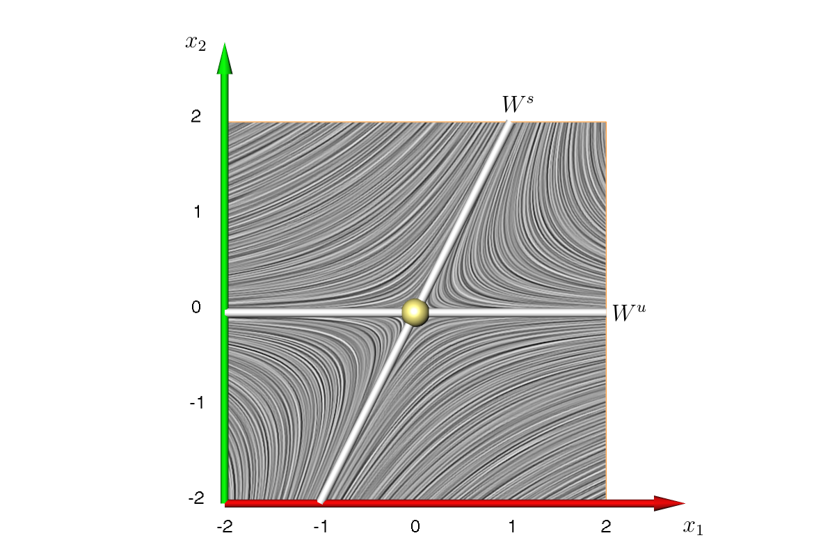
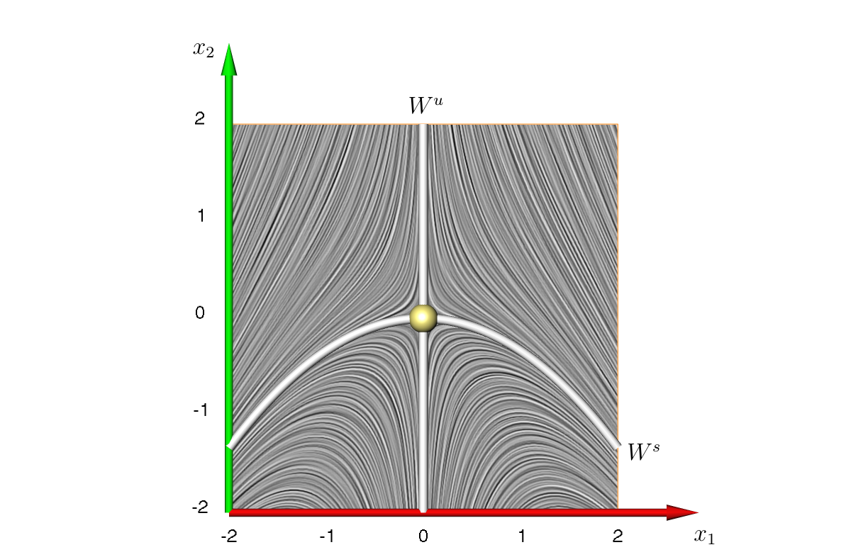
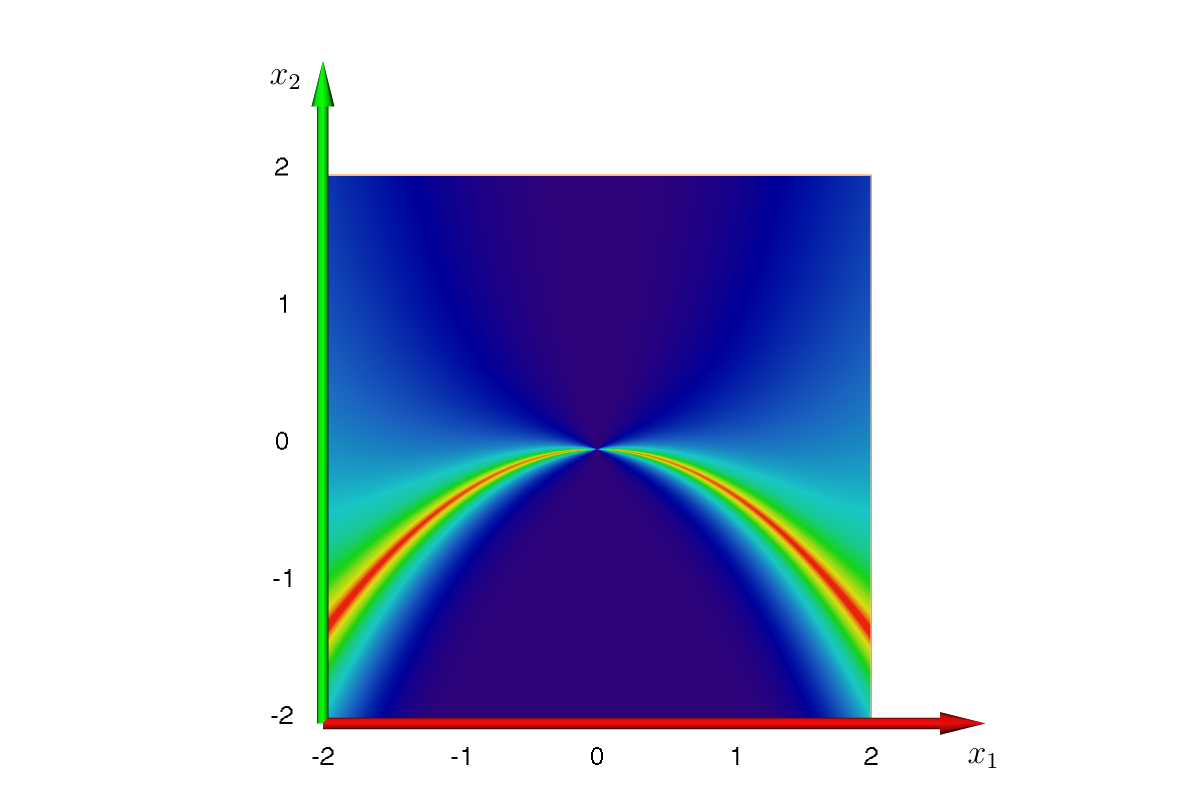
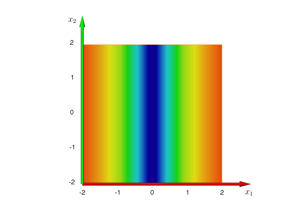
exhibits ridge and trough-like coherent structures which approach classical invariant manifolds as T→∞T\to\infty. Figure 2 shows the weighted FTME field (30) for the linear differential equation x˙1=x1−x2\dot{x}_{1}=x_{1}-x_{2}, x˙2=−x2\dot{x}_{2}=-x_{2}, with stable manifold Ws={(x1,x2)∈ℝ2:2​x1=x2}W^{s}=\{(x_{1},x_{2})\in\mathbb{R}^{2}:2x_{1}=x_{2}\} and unstable manifold Wu={(x1,x2)∈ℝ2:x2=0}W^{u}=\{(x_{1},x_{2})\in\mathbb{R}^{2}:x_{2}=0\}. Figure 4 shows the weighted FTME field (30) for the nonlinear differential equation x˙1=−x1\dot{x}_{1}=-x_{1}, x˙2=x12+x2\dot{x}_{2}=x_{1}^{2}+x_{2}. Its unstable manifold Wu={(x1,x2)∈ℝ2:x1=0}W^{u}=\{(x_{1},x_{2})\in\mathbb{R}^{2}:x_{1}=0\} is the x2x_{2}-axis and its stable manifold Wu={(x1,x2)∈ℝ2:x2=13​x12}W^{u}=\{(x_{1},x_{2})\in\mathbb{R}^{2}:x_{2}=\frac{1}{3}x_{1}^{2}\} is a parabola.

Instead of developing a complete theory for ridge-like structures of weighted FTME fields in this section, we take advantage of the fact that for the specific classes of examples which we discuss in this section, the points xx in the ridge and trough-like structures of the weighted FTME field (30) satisfy the condition ∇H​(x)=0\nabla H(x)=0. Using Proposition 13(ii) with the abbreviations κ1​(x):=e(λ1​(x,T)−α⁡(x,T,f⁡(x)))​T\kappa_{1}(x):=e^{(\lambda_{1}(x,T)-\alpha(x,T,f(x)))T} and κ2​(x):=e(λ2​(x,T)−α⁡(x,T,f⁡(x)))​T\kappa_{2}(x):=e^{(\lambda_{2}(x,T)-\alpha(x,T,f(x)))T}, and using the fact that α⁡(x,T,f⁡(x))∈[λ2​(x,T),λ1​(x,T)]\alpha(x,T,f(x))\in[\lambda_{2}(x,T),\lambda_{1}(x,T)] and hence κ1​(x)>1>κ2​(x)\kappa_{1}(x)>1>\kappa_{2}(x), we get H⁡(x)=h⁡(κ1​(x),κ2​(x))H(x)=h(\kappa_{1}(x),\kappa_{2}(x)) with h⁡(κ1,κ2)=−1T​log⁡2π​(arccos⁡κ12−1κ12−κ22+1κ1​κ2​arccos⁡κ1​1−κ22κ12−κ22)h(\kappa_{1},\kappa_{2})=-\frac{1}{T}\log\frac{2}{\pi}\left(\arccos\sqrt{\frac{\kappa_{1}^{2}-1}{\kappa_{1}^{2}-\kappa_{2}^{2}}}+\frac{1}{\kappa_{1}\kappa_{2}}\arccos\kappa_{1}\sqrt{\frac{1-\kappa_{2}^{2}}{\kappa_{1}^{2}-\kappa_{2}^{2}}}\right) and hence

∇H​(x)\displaystyle\nabla H(x) =\displaystyle= ∂h∂κ1​(κ1​(x),κ2​(x))​κ1​(x)​T​(∇λ1​(x,T)−∇α​(x,T,f⁡(x)))\displaystyle\tfrac{\partial h}{\partial\kappa_{1}}\big(\kappa_{1}(x),\kappa_{2}(x)\big)\kappa_{1}(x)T\big(\nabla\lambda_{1}(x,T)-\nabla\alpha(x,T,f(x))\big) (31)
+∂h∂κ2​(κ1​(x),κ2​(x))​κ2​(x)​T​(∇λ2​(x,T)−∇α​(x,T,f⁡(x))).\displaystyle{}+\tfrac{\partial h}{\partial\kappa_{2}}\big(\kappa_{1}(x),\kappa_{2}(x)\big)\kappa_{2}(x)T\big(\nabla\lambda_{2}(x,T)-\nabla\alpha(x,T,f(x))\big).

Note that in higher dimensions the weighted FTME field (30) could fail to be C1C^{1} for xx in a lower-dimensional subset (cp. Kato [15]).

We will present two examples below which both satisfy the assumption that ∇(λ1​(x,T)+λ2​(x,T))=0\nabla\big(\lambda_{1}(x,T)+\lambda_{2}(x,T)\big)=0. In this case, finding the zeros of ∇H​(x)\nabla H(x) in (31) is equivalent to solving

(∂h∂κ1(κ1(x),κ2(x))κ1(x)−∂h∂κ2(κ1(x),κ2(x))κ2(x))∇λ1(x,T)\displaystyle\Big(\frac{\partial h}{\partial\kappa_{1}}\big(\kappa_{1}(x),\kappa_{2}(x)\big)\kappa_{1}(x)-\frac{\partial h}{\partial\kappa_{2}}\big(\kappa_{1}(x),\kappa_{2}(x)\big)\kappa_{2}(x)\Big)\nabla\lambda_{1}(x,T) (32)
=\displaystyle= (∂h∂κ1(κ1(x),κ2(x))κ1(x)+∂h∂κ2(κ1(x),κ2(x))κ2(x))∇α(x,T,f(x)).\displaystyle\Big(\frac{\partial h}{\partial\kappa_{1}}\big(\kappa_{1}(x),\kappa_{2}(x)\big)\kappa_{1}(x)+\frac{\partial h}{\partial\kappa_{2}}\big(\kappa_{1}(x),\kappa_{2}(x)\big)\kappa_{2}(x)\Big)\nabla\alpha(x,T,f(x)).
Example 17.

Consider a two dimensional linear autonomous system

x˙=A​x\dot{x}=Ax (33)

with a matrix A∈ℝ2×2A\in\mathbb{R}^{2\times 2} which has two eigenvalues λ1>0>λ2\lambda_{1}>0>\lambda_{2} and corresponding eigenvectors e1,e2e_{1},e_{2}. The solution of the initial value problem (33), x⁡(0)=x0x(0)=x_{0}, is φ⁡(t,x0)=eA​t​x0\varphi(t,x_{0})=e^{At}x_{0}, and the system has unstable and stable manifolds WuW^{u} and WsW^{s} which are two lines with directional vectors e1e_{1} and e2e_{2}. The linearized solution Φ⁡(t)=Φx0​(t):=Dx0​φ​(t,x0)=eA​t\Phi(t)=\Phi_{x_{0}}(t):=D_{x_{0}}\varphi(t,x_{0})=e^{At} is independent of x0x_{0}. We consider (33) for t∈[0,T]t\in[0,T] for arbitrary T>0T>0. It follows that the FTLE λi​(T)=λi​(x0,T)\lambda_{i}(T)=\lambda_{i}(x_{0},T) are also independent of x0x_{0}, i.e. ∇λi​(x0,T)=(0,0)\nabla\lambda_{i}(x_{0},T)=(0,0) for i=1,2i=1,2. In particular the FTLE field x0↦λ1​(x0,T)x_{0}\mapsto\lambda_{1}(x_{0},T) is constant and not capable of detecting any coherent structures such as stable or unstable manifolds.

Refer to caption

Figure 1: Vector field and invariant manifolds WsW^{s} and WuW^{u} for x˙1=x1−x2\dot{x}_{1}=x_{1}-x_{2}, x˙2=−x2\dot{x}_{2}=-x_{2}.

Refer to caption

Figure 2: Weighted FTME field (30) for x˙1=x1−x2\dot{x}_{1}=x_{1}-x_{2}, x˙2=−x2\dot{x}_{2}=-x_{2} (blue ≃0\simeq 0, red ≃1\simeq 1).

The solutions x0x_{0} of (32) are given by the zeros of ∇α​(x0)\nabla\alpha(x_{0}), where α⁡(x0)=α⁡(x0,T,A​x0)=1T​log⁡‖Φ⁡(T)​A​x0‖‖A​x0‖\alpha(x_{0})=\alpha(x_{0},T,Ax_{0})=\frac{1}{T}\log\frac{\|\Phi(T)Ax_{0}\|}{\|Ax_{0}\|}. It follows that

0\displaystyle 0 =\displaystyle= ∇α(x0)=1T‖A​x0‖‖Φ⁡(T)​A​x0‖∇(‖Φ⁡(T)​A​x0‖‖A​x0‖)\displaystyle\nabla\alpha(x_{0})=\frac{1}{T}\frac{\|Ax_{0}\|}{\|\Phi(T)Ax_{0}\|}\nabla\Big(\frac{\|\Phi(T)Ax_{0}\|}{\|Ax_{0}\|}\Big)
=\displaystyle= 1T​1‖Φ⁡(T)​A​x0‖2​AT​(Φ​(T)T​Φ​(T)​A​x0−‖Φ⁡(T)​A​x0‖2‖A​x0‖2​A​x0)\displaystyle\frac{1}{T}\frac{1}{\|\Phi(T)Ax_{0}\|^{2}}A^{\mathrm{T}}\Big(\Phi(T)^{\mathrm{T}}\Phi(T)Ax_{0}-\frac{\|\Phi(T)Ax_{0}\|^{2}}{\|Ax_{0}\|^{2}}Ax_{0}\Big)

and hence A​x0Ax_{0} is an eigenvector of Φ​(T)T​Φ​(T)\Phi(T)^{\mathrm{T}}\Phi(T). Let U=(e1|e2)U=(e_{1}|e_{2}) denote the matrix whose column vectors are e1e_{1} and e2e_{2}, thus A=U​diag⁡(λ1,λ2)​U−1A=U\diag(\lambda_{1},\lambda_{2})U^{-1}. We then have

λ1​(T)\displaystyle\lambda_{1}(T) =\displaystyle= 1T​log|Φ⁡(T)|=1T​log​‖U​diag⁡(eλ1​T,eλ2​T)​U−1‖,\displaystyle\frac{1}{T}\log\|\Phi(T)\|=\frac{1}{T}\log\|U\diag(e^{\lambda_{1}T},e^{\lambda_{2}T})U^{-1}\|,
λ2​(T)\displaystyle\lambda_{2}(T) =\displaystyle= 1T​log|Φ​(T)−1|=1T​log⁡‖U​diag⁡(e−λ1​T,e−λ2​T)​U−1‖.\displaystyle\frac{1}{T}\log\|\Phi(T)^{-1}\|=\frac{1}{T}\log\|U\diag(e^{-\lambda_{1}T},e^{-\lambda_{2}T})U^{-1}\|.

A direct computation shows that for ε>0\varepsilon>0 and T>log⁡‖U‖+log⁡‖U−1‖εT>\frac{\log\|U\|+\log\|U^{-1}\|}{\varepsilon} the estimate

|λi​(T)−λi|≤1T​(log⁡‖U‖+log⁡‖U−1‖)≤εfor ​i=1,2|\lambda_{i}(T)-\lambda_{i}|\leq\frac{1}{T}\big(\log\|U\|+\log\|U^{-1}\|\big)\leq\varepsilon\qquad\text{for }i=1,2

holds.

For i=1,2i=1,2 let vi​(T)=vi​(x0,T)v_{i}(T)=v_{i}(x_{0},T) with ‖vi​(T)‖=1\|v_{i}(T)\|=1 denote the finite-time Lyapunov vectors corresponding to λi​(T)\lambda_{i}(T), i.e. Φ​(T)T​Φ​(T)​vi​(T)=λi​(T)​vi​(T)\Phi(T)^{\mathrm{T}}\Phi(T)v_{i}(T)=\lambda_{i}(T)v_{i}(T). Since e2=⟨e2,v1​(T)⟩​v1​(T)+⟨e2,v2​(T)⟩​v2​(T)e_{2}=\langle e_{2},v_{1}(T)\rangle v_{1}(T)+\langle e_{2},v_{2}(T)\rangle v_{2}(T), we get

e2​λ2​T\displaystyle e^{2\lambda_{2}T} =\displaystyle= ‖Φ⁡(T)​e2‖2=⟨e2,Φ​(T)T​Φ​(T)​e2⟩\displaystyle\|\Phi(T)e_{2}\|^{2}=\langle e_{2},\Phi(T)^{\mathrm{T}}\Phi(T)e_{2}\rangle
=\displaystyle= ⟨e2,v1​(T)⟩2​e2​λ1​(T)​T+⟨e2,v2​(T)⟩2​e2​λ2​(T)​T.\displaystyle\langle e_{2},v_{1}(T)\rangle^{2}e^{2\lambda_{1}(T)T}+\langle e_{2},v_{2}(T)\rangle^{2}e^{2\lambda_{2}(T)T}.

Hence |⟨e2,v1​(T)⟩|≤e(λ2−λ1​(T))​T≤e(λ2−λ1+ε)​T|\langle e_{2},v_{1}(T)\rangle|\leq e^{(\lambda_{2}-\lambda_{1}(T))T}\leq e^{(\lambda_{2}-\lambda_{1}+\varepsilon)T} or |sin⁡∠⁡(e2,v2​(T))|≤e(λ2−λ1+ε)​T|\sin\angle(e_{2},v_{2}(T))|\leq e^{(\lambda_{2}-\lambda_{1}+\varepsilon)T}.

Assume that A​x0|v2​(T)Ax_{0}\parallel v_{2}(T), the case A​x0|v1​(T)Ax_{0}\parallel v_{1}(T) is analog. Then |sin⁡∠⁡(e2,A​x0‖A​x0‖)|≤e(λ2−λ1+ε)​T|\sin\angle(e_{2},\frac{Ax_{0}}{\|Ax_{0}\|})|\leq e^{(\lambda_{2}-\lambda_{1}+\varepsilon)T}. Since A​e2=λ2​e2Ae_{2}=\lambda_{2}e_{2}, it follows that |sin⁡∠⁡(e2,x0‖x0‖)|≤e(λ2−λ1+ϵ)​T|\sin\angle(e_{2},\frac{x_{0}}{\|x_{0}\|})|\leq e^{(\lambda_{2}-\lambda_{1}+\epsilon)T}. In other words, the ridge and trough of the weighted FTME field x0↦H⁡(x0)x_{0}\mapsto H(x_{0}) of system (33) are the two lines which are defined by the zeros of ∇H​(x0)\nabla H(x_{0}) and converge to the stable and unstable invariant manifolds for T→∞T\to\infty, see also the vector field in Figure 2 and the weighted FTME field of (33) in Figure 2 for A=(1−10−1)A={1\;-1\choose 0\;-1}.

Example 18.

For γ,β∈ℝ\gamma,\beta\in\mathbb{R}, γ>0\gamma>0, consider the following family of autonomous differential equations

x˙1=−x1,x˙2=β​x12+γ​x2.\begin{array}[]{rcl}\dot{x}_{1}&=&-x_{1},\\ \dot{x}_{2}&=&\beta x_{1}^{2}+\gamma x_{2}.\end{array} (34)

Its solution for t∈ℝt\in\mathbb{R} and x0=(x01,x02)∈ℝ2x_{0}=(x_{01},x_{02})\in\mathbb{R}^{2} is given by

φ⁡(t,x0)={e−t​x01β2+γ​x012​(eγ​t−e−2​t)+eγ​t​x02\varphi(t,x_{0})=\left\{\begin{array}[]{l}e^{-t}x_{01}\\ \frac{\beta}{2+\gamma}x_{01}^{2}(e^{\gamma t}-e^{-2t})+e^{\gamma t}x_{02}\end{array}\right.

and its linearization Φx0​(t)=Dx0​φ​(t,x0)\Phi_{x_{0}}(t)=D_{x_{0}}\varphi(t,x_{0}) is

Φx0​(t)=(e−t02​β2+γ​x01​(eγ​t−e−2​t)eγ​t)=:(a0bc).\displaystyle\Phi_{x_{0}}(t)=\left(\begin{array}[]{ccc}e^{-t}&0\\ \frac{2\beta}{2+\gamma}x_{01}(e^{\gamma t}-e^{-2t})&e^{\gamma t}\end{array}\right)=:\left(\begin{array}[]{ccc}a&0\\ b&c\end{array}\right).

System (34) has an equilibrium at the origin with invariant stable and unstable manifolds

Ws\displaystyle W^{s} =\displaystyle= {(x01,x02)∈ℝ2:x02+β2+γ​x012=0},\displaystyle\big\{(x_{01},x_{02})\in\mathbb{R}^{2}:x_{02}+\tfrac{\beta}{2+\gamma}x_{01}^{2}=0\big\},
Wu\displaystyle W^{u} =\displaystyle= {(x01,x02)∈ℝ2:x01=0}.\displaystyle\big\{(x_{01},x_{02})\in\mathbb{R}^{2}:x_{01}=0\big\}.

We consider (34) for t∈[0,T]t\in[0,T] for an arbitrary T>0T>0. Its FTLEs λi​(x0,T)\lambda_{i}(x_{0},T) for i=1,2i=1,2 are

λi​(x0,T)=12​T​log⁡Λi​(x0,T)with ​Λi​(x0,T)=a2+b2+c2±[(a2+b2+c2)2−4]122.\lambda_{i}(x_{0},T)=\frac{1}{2T}\log\Lambda_{i}(x_{0},T)\quad\text{with }\Lambda_{i}(x_{0},T)=\frac{a^{2}+b^{2}+c^{2}\pm[(a^{2}+b^{2}+c^{2})^{2}-4]^{\frac{1}{2}}}{2}.

Thus λ1​(x0,T)\lambda_{1}(x_{0},T) depends only on x01x_{01}, i.e. ∂λ1​(x0,T)∂x02=0\frac{\partial\lambda_{1}(x_{0},T)}{\partial x_{02}}=0. By (32), the zeros of ∇H​(x0)\nabla H(x_{0}) are the solutions to

(∂h∂κ1​(κ1​(x),κ2​(x))​κ1​(x)−∂h∂κ2​(κ1​(x),κ2​(x))​κ2​(x))​(∂Λ1​(x0,T)∂x01,0)2​T​Λ1​(x0,T)\displaystyle\Big(\frac{\partial h}{\partial\kappa_{1}}\big(\kappa_{1}(x),\kappa_{2}(x)\big)\kappa_{1}(x)-\frac{\partial h}{\partial\kappa_{2}}\big(\kappa_{1}(x),\kappa_{2}(x)\big)\kappa_{2}(x)\Big)\frac{\big(\frac{\partial\Lambda_{1}(x_{0},T)}{\partial x_{01}},0\big)}{2T\Lambda_{1}(x_{0},T)} (36)
=\displaystyle= (∂h∂α1​(α1​(x),α2​(x))​α1​(x)+∂h∂α2​(α1​(x),α2​(x))​α2​(x))​(∂g⁡(x0)∂x01,∂g⁡(x0)∂x02)2​T​g​(x0),\displaystyle\Big(\frac{\partial h}{\partial\alpha_{1}}\big(\alpha_{1}(x),\alpha_{2}(x)\big)\alpha_{1}(x)+\frac{\partial h}{\partial\alpha_{2}}\big(\alpha_{1}(x),\alpha_{2}(x)\big)\alpha_{2}(x)\Big)\frac{\big(\frac{\partial g(x_{0})}{\partial x_{01}},\frac{\partial g(x_{0})}{\partial x_{02}}\big)}{2Tg(x_{0})},

where

g⁡(x0)=‖Φx0​(T)​f​(x0)‖2‖f⁡(x0)‖2=e−2​T​x012+[γ​eγ​T​x02+γ​β2+γ​(eγ​T−e−2​T)​x012+β​e−2​T​x012]2x012+(γ​x02+β​x012)2.g(x_{0})=\frac{\|\Phi_{x_{0}}(T)f(x_{0})\|^{2}}{\|f(x_{0})\|^{2}}=\frac{e^{-2T}x_{01}^{2}+\big[\gamma e^{\gamma T}x_{02}+\frac{\gamma\beta}{2+\gamma}(e^{\gamma T}-e^{-2T})x_{01}^{2}+\beta e^{-2T}x_{01}^{2}\big]^{2}}{x_{01}^{2}+(\gamma x_{02}+\beta x_{01}^{2})^{2}}.

Equation (36) implies ∂g∂x02=0\frac{\partial g}{\partial x_{02}}=0, which yields

2​γ​eγ​T​[γ​eγ​T​x02+γ​β2+γ​(eγ​T−e−2​T)​x012+β​e−2​T​x012]​[x012+(γ​x02+β​x012)2]\displaystyle 2\gamma e^{\gamma T}\big[\gamma e^{\gamma T}x_{02}+\tfrac{\gamma\beta}{2+\gamma}(e^{\gamma T}-e^{-2T})x_{01}^{2}+\beta e^{-2T}x_{01}^{2}\big]\big[x_{01}^{2}+(\gamma x_{02}+\beta x_{01}^{2})^{2}\big] (37)
=\displaystyle= 2​γ​(γ​x02+β​x012)​{e−2​T​x012+[γ​eγ​T​x02+γ​β2+γ​(eγ​T−e−2​T)​x012+β​e−2​T​x012]2}.\displaystyle 2\gamma(\gamma x_{02}+\beta x_{01}^{2})\big\{e^{-2T}x_{01}^{2}+\big[\gamma e^{\gamma T}x_{02}+\tfrac{\gamma\beta}{2+\gamma}(e^{\gamma T}-e^{-2T})x_{01}^{2}+\beta e^{-2T}x_{01}^{2}\big]^{2}\big\}.

Dividing both sides of (37) by e2​γ​Te^{2\gamma T}, we get

x012​(x02+β2+γ​x012)​(x02+βγ​x012+2+γ2​γ​β)=e−(1+2​γ)​T​h​(x01,x02),x_{01}^{2}\big(x_{02}+\tfrac{\beta}{2+\gamma}x_{01}^{2}\big)\big(x_{02}+\tfrac{\beta}{\gamma}x_{01}^{2}+\tfrac{2+\gamma}{2\gamma\beta}\big)=e^{-(1+2\gamma)T}h(x_{01},x_{02}), (38)

where h⁡(x10,x20)h(x_{10},x_{20}) is a polynomial in x10x_{10} and x20x_{20}. Since the right hand side of (38) tends to 00 as T→∞T\to\infty, the solutions x0=(x01,x02)x_{0}=(x_{01},x_{02}) of equation (38) satisfies either x01≈0x_{01}\approx 0 or x02+β2+γ​x012≈0x_{02}+\frac{\beta}{2+\gamma}x_{01}^{2}\approx 0 or x02+βγ​x012+2+γ2​γ​β≈0x_{02}+\frac{\beta}{\gamma}x_{01}^{2}+\frac{2+\gamma}{2\gamma\beta}\approx 0 for TT large. Finally, by solving the first component of (36), we conclude that the zeros x0x_{0} of ∇H​(x0)\nabla H(x_{0}) satisfy either x01→0x_{01}\to 0 or x02+β2+γ​x012→0x_{02}+\frac{\beta}{2+\gamma}x_{01}^{2}\to 0 for T→∞T\to\infty, proving that the rigde and trough-like structures of the weighted FTME field x0↦H⁡(x0)x_{0}\mapsto H(x_{0}) are finite-time approximations of the stable and unstable manifold, see also the vector field and weighted FTME field of (38) for γ=β=1\gamma=\beta=1 in Figures 4 and 4.

Refer to caption

Figure 3: Vector field and invariant manifolds WsW^{s} and WuW^{u} for x˙1=−x1\dot{x}_{1}=-x_{1}, x˙2=x12+x2\dot{x}_{2}=x_{1}^{2}+x_{2}.

Refer to caption

Figure 4: Weighted FTME field (30) for x˙1=−x1\dot{x}_{1}=-x_{1}, x˙2=x12+x2\dot{x}_{2}=x_{1}^{2}+x_{2} with T=2T=2 (blue ≃0\simeq 0, red ≃2.25\simeq 2.25).

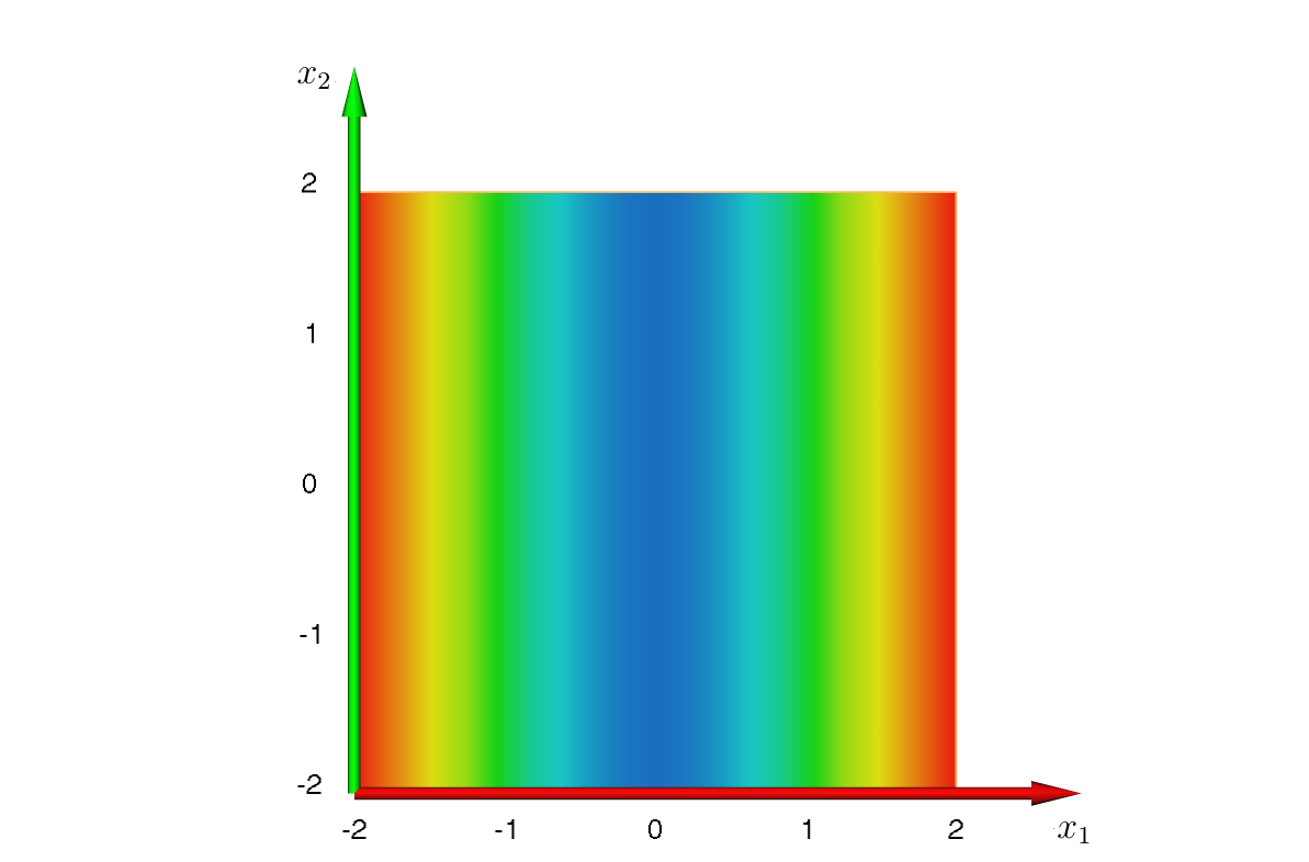
As can be seen in Figures 6 and 6, the forward and backward FTLE fields are not capable of detecting the stable manifold of (38) for γ=β=1\gamma=\beta=1. In fact, a smooth compact curve ℳ⁡(t)⊂ℝ2\mathcal{M}(t)\subset\mathbb{R}^{2} at time t0t_{0} needs to satisfy conditions 2 and 3 of Theorem 2(i) in order to qualify as a candidate for a weak LCS. This is equivalent to ∇λ1(x0,T)T∥Tx0M(t0)\nabla\lambda_{1}(x_{0},T)^{\mathrm{T}}\parallel T_{x_{0}}M(t_{0}). Since ∂λ1​(x0,T)∂x02=0\frac{\partial\lambda_{1}(x_{0},T)}{\partial x_{02}}=0, this is equivalent to Tx0​ℳ​(t0)|(1,0)TT_{x_{0}}\mathcal{M}(t_{0})\parallel(1,0)^{\mathrm{T}}. Hence the possible repelling LCS candidates can only be lines which are parallel to the x01x_{01} axis, in constrast to the stable manifold Ws={(x01,x02)∈ℝ2:x02+β2+γ​x012=0}W^{s}=\big\{(x_{01},x_{02})\in\mathbb{R}^{2}:x_{02}+\tfrac{\beta}{2+\gamma}x_{01}^{2}=0\big\} of (38) which is a parabola.

Refer to caption

Figure 5: Forward FTLE field x0↦λ1​(x0,T)x_{0}\mapsto\lambda_{1}(x_{0},T) for x˙1=−x1\dot{x}_{1}=-x_{1}, x˙2=x12+x2\dot{x}_{2}=x_{1}^{2}+x_{2} with T=2T=2 (blue ≃0.9\simeq 0.9, red ≃1.25\simeq 1.25).

Refer to caption

Figure 6: Backward FTLE field for x˙1=−x1\dot{x}_{1}=-x_{1}, x˙2=x12+x2\dot{x}_{2}=x_{1}^{2}+x_{2} on [−2,0][-2,0] (blue ≃0.9\simeq 0.9, red ≃2.2\simeq 2.2).

The two examples 17 and 18 illustrate that ridge and trough-like structures of the weighted FTME field approximate classical stable and unstable manifolds. In the remainder of this section we show that also for arbitrary two-dimensional systems (28) the weighted FTME field is capable of detecting invariant manifolds in the vicinity of equilibria. The following preparatory lemma provides an estimate for the stretching rate (29) near an isolated equilibrium x∗x^{*}.

Lemma 19 (Directional stretching rate in direction of vector field close to equilibrium).

Assume that (28) has an isolated equilibrium x∗x^{*}. Then its directional stretching rate α⁡(x0):=α⁡(x0,T,f⁡(x0))\alpha(x_{0}):=\alpha(x_{0},T,f(x_{0})) for x0≠x∗x_{0}\neq x^{*} can be approximated in the following sense

limx0→x∗|α⁡(x0)−1T​log⁡‖Φx∗​(T)​(x0−x∗)‖‖x0−x∗‖|≤1T​(log⁡‖Dx​f​(x∗)‖+log⁡‖Dx​f​(x∗)−1‖).\lim_{x_{0}\to x^{*}}\Big|\alpha(x_{0})-\frac{1}{T}\log\frac{\|\Phi_{x^{*}}(T)(x_{0}-x^{*})\|}{\|x_{0}-x^{*}\|}\Big|\leq\frac{1}{T}\big(\log\|D_{x}f(x^{*})\|+\log\|D_{x}f(x^{*})^{-1}\|\big). (39)
Proof.

To estimate the stretching rate, observe that for x0≠x∗x_{0}\neq x^{*} with f⁡(x0)≠0f(x_{0})\neq 0

α⁡(x0)\displaystyle\alpha(x_{0}) =\displaystyle= 1T​log⁡‖Φx0​(T)​f​(x0)‖‖f⁡(x0)‖\displaystyle\frac{1}{T}\log\frac{\|\Phi_{x_{0}}(T)f(x_{0})\|}{\|f(x_{0})\|}
=\displaystyle= 1T​log⁡‖Φx∗​(T)​f​(x0)‖f⁡(x0)‖+[Φx0​(T)−Φx∗​(T)]​f​(x0)‖f⁡(x0)‖‖\displaystyle\frac{1}{T}\log\Big\|\frac{\Phi_{x^{*}}(T)f(x_{0})}{\|f(x_{0})\|}+\frac{[\Phi_{x_{0}}(T)-\Phi_{x^{*}}(T)]f(x_{0})}{\|f(x_{0})\|}\Big\|
=\displaystyle= 1T​log⁡‖Φx∗​(T)​f​(x0)‖f⁡(x0)‖+g⁡(T,x0−x∗)​f⁡(x0)‖f⁡(x0)‖‖\displaystyle\frac{1}{T}\log\Big\|\frac{\Phi_{x^{*}}(T)f(x_{0})}{\|f(x_{0})\|}+g(T,x_{0}-x^{*})\frac{f(x_{0})}{\|f(x_{0})\|}\Big\|
=\displaystyle= 1T​log|Φx∗​(T)​[f⁡(x∗)+Dx​f​(x∗)​(x0−x∗)+h⁡(T,x0−x∗)​(x0−x∗)]‖f⁡(x∗)+Dx​f​(x∗)​(x0−x∗)+h⁡(T,x0−x∗)​(x0−x∗)‖\displaystyle\frac{1}{T}\log\Big\|\frac{\Phi_{x^{*}}(T)[f(x^{*})+D_{x}f(x^{*})(x_{0}-x^{*})+h(T,x_{0}-x^{*})(x_{0}-x^{*})]}{\|f(x^{*})+D_{x}f(x^{*})(x_{0}-x^{*})+h(T,x_{0}-x^{*})(x_{0}-x^{*})\|}
+g(T,x0−x∗)f⁡(x0)‖f⁡(x0)‖∥\displaystyle{}+g(T,x_{0}-x^{*})\frac{f(x_{0})}{\|f(x_{0})\|}\Big\|
=\displaystyle= 1T​log|Φx∗​(T)​[Dx​f​(x∗)​(x0−x∗)+h⁡(T,x0−x∗)​(x0−x∗)]‖Dx​f​(x∗)​(x0−x∗)+h⁡(T,x0−x∗)​(x0−x∗)‖\displaystyle\frac{1}{T}\log\Big\|\frac{\Phi_{x^{*}}(T)[D_{x}f(x^{*})(x_{0}-x^{*})+h(T,x_{0}-x^{*})(x_{0}-x^{*})]}{\|D_{x}f(x^{*})(x_{0}-x^{*})+h(T,x_{0}-x^{*})(x_{0}-x^{*})\|}
+g(T,x0−x∗)f⁡(x0)‖f⁡(x0)‖∥\displaystyle{}+g(T,x_{0}-x^{*})\frac{f(x_{0})}{\|f(x_{0})\|}\Big\|
=\displaystyle= 1T​log⁡‖Φx∗​(T)​[Dx​f​(x∗)​(x0−x∗)‖Dx​f​(x∗)​(x0−x∗)‖+h⁡(T,x0−x∗)​(x0−x∗)‖Dx​f​(x∗)​(x0−x∗)‖]‖Dx​f​(x∗)​(x0−x∗)‖Dx​f​(x∗)​(x0−x∗)‖+h⁡(T,x0−x∗)​(x0−x∗)‖Dx​f​(x∗)​(x0−x∗)‖‖+g⁡(T,x0−x∗)​f⁡(x0)‖f⁡(x0)‖‖\displaystyle\frac{1}{T}\log\Big\|\frac{\Phi_{x^{*}}(T)[\frac{D_{x}f(x^{*})(x_{0}-x^{*})}{\|D_{x}f(x^{*})(x_{0}-x^{*})\|}+\frac{h(T,x_{0}-x^{*})(x_{0}-x^{*})}{\|D_{x}f(x^{*})(x_{0}-x^{*})\|}]}{\|\frac{D_{x}f(x^{*})(x_{0}-x^{*})}{\|D_{x}f(x^{*})(x_{0}-x^{*})\|}+\frac{h(T,x_{0}-x^{*})(x_{0}-x^{*})}{\|D_{x}f(x^{*})(x_{0}-x^{*})\|}\|}+g(T,x_{0}-x^{*})\frac{f(x_{0})}{\|f(x_{0})\|}\Big\|

where g⁡(T,x0−x∗),h⁡(T,x0−x∗)∈ℝng(T,x_{0}-x^{*}),h(T,x_{0}-x^{*})\in\mathbb{R}^{n} satisfy limx0→x∗g⁡(T,x0−x∗)=limx0→x∗h⁡(T,x0−x∗)=0\lim\limits_{x_{0}\to x^{*}}g(T,x_{0}-x^{*})=\lim\limits_{x_{0}\to x^{*}}h(T,x_{0}-x^{*})=0. Since limx0→x∗‖g⁡(T,x0−x∗)​f⁡(x0)‖f⁡(x0)‖‖=0\lim\limits_{x_{0}\to x^{*}}\|g(T,x_{0}-x^{*})\frac{f(x_{0})}{\|f(x_{0})\|}\|=0 and

limx0→x∗h⁡(T,x0−x∗)​(x0−x∗)‖Dx​f​(x∗)​(x0−x∗)‖=limx0→x∗h⁡(T,x0−x∗)​x0−x∗‖x0−x∗‖‖Dx​f​(x∗)​(x0−x∗)‖x0−x∗‖‖=0,\lim\limits_{x_{0}\to x^{*}}\frac{h(T,x_{0}-x^{*})(x_{0}-x^{*})}{\|D_{x}f(x^{*})(x_{0}-x^{*})\|}=\lim\limits_{x_{0}\to x^{*}}\frac{h(T,x_{0}-x^{*})\frac{x_{0}-x^{*}}{\|x_{0}-x^{*}\|}}{\|D_{x}f(x^{*})\frac{(x_{0}-x^{*})}{\|x_{0}-x^{*}\|}\|}=0,

we have

limx0→x∗α⁡(x0)−1T​log⁡‖Φx∗​(T)​Dx​f​(x∗)​(x0−x∗)‖‖Dx​f​(x∗)​(x0−x∗)‖=0.\lim_{x_{0}\to x^{*}}\alpha(x_{0})-\frac{1}{T}\log\frac{\|\Phi_{x^{*}}(T)D_{x}f(x^{*})(x_{0}-x^{*})\|}{\|D_{x}f(x^{*})(x_{0}-x^{*})\|}=0.

Using the fact that Φx∗​(T)​Dx​f​(x∗)=eDx​f​(x∗)​T​Dx​f​(x∗)=Dx​f​(x∗)​eDx​f​(x∗)​T=Dx​f​(x∗)​Φx∗​(T)\Phi_{x^{*}}(T)D_{x}f(x^{*})=e^{D_{x}f(x^{*})T}D_{x}f(x^{*})=D_{x}f(x^{*})e^{D_{x}f(x^{*})T}=D_{x}f(x^{*})\Phi_{x^{*}}(T) and the estimates

‖Φx∗​(T)​(x0−x∗)‖‖Dx​f​(x∗)−1‖\displaystyle\frac{\|\Phi_{x^{*}}(T)(x_{0}-x^{*})\|}{\|D_{x}f(x^{*})^{-1}\|} ≤\displaystyle\leq ‖Dx​f​(x∗)​Φx∗​(T)​(x0−x∗)‖≤‖Dx​f​(x∗)‖​‖Φx∗​(T)​(x0−x∗)‖,\displaystyle\|D_{x}f(x^{*})\Phi_{x^{*}}(T)(x_{0}-x^{*})\|\leq\|D_{x}f(x^{*})\|\|\Phi_{x^{*}}(T)(x_{0}-x^{*})\|,
‖x0−x∗‖‖Dx​f​(x∗)−1‖\displaystyle\frac{\|x_{0}-x^{*}\|}{\|D_{x}f(x^{*})^{-1}\|} ≤\displaystyle\leq ‖Dx​f​(x∗)​(x0−x∗)‖≤‖Dx​f​(x∗)‖​‖(x0−x∗)‖,\displaystyle\|D_{x}f(x^{*})(x_{0}-x^{*})\|\leq\|D_{x}f(x^{*})\|\|(x_{0}-x^{*})\|,

it follows that

‖Φx∗​(T)​(x0−x∗)‖‖Dx​f​(x∗)‖​‖Dx​f​(x∗)−1‖​‖x0−x∗‖\displaystyle\frac{\|\Phi_{x^{*}}(T)(x_{0}-x^{*})\|}{\|D_{x}f(x^{*})\|\|D_{x}f(x^{*})^{-1}\|\|x_{0}-x^{*}\|} ≤\displaystyle\leq ‖Dx​f​(x∗)​Φx∗​(T)​(x0−x∗)‖‖Dx​f​(x∗)​(x0−x∗)‖\displaystyle\frac{\|D_{x}f(x^{*})\Phi_{x^{*}}(T)(x_{0}-x^{*})\|}{\|D_{x}f(x^{*})(x_{0}-x^{*})\|}
≤\displaystyle\leq ‖Φx∗​(T)​(x0−x∗)‖​‖Dx​f​(x∗)‖​‖Dx​f​(x∗)−1‖,\displaystyle\|\Phi_{x^{*}}(T)(x_{0}-x^{*})\|\|D_{x}f(x^{*})\|\|D_{x}f(x^{*})^{-1}\|,

or equivalently

|1T​log⁡‖Φx∗​(T)​Dx​f​(x∗)​(x0−x∗)‖‖Dx​f​(x∗)​(x0−x∗)‖−1T​log⁡‖Φx∗​(T)​(x0−x∗)‖‖x0−x∗‖|\displaystyle\Big|\frac{1}{T}\log\frac{\|\Phi_{x^{*}}(T)D_{x}f(x^{*})(x_{0}-x^{*})\|}{\|D_{x}f(x^{*})(x_{0}-x^{*})\|}-\frac{1}{T}\log\frac{\|\Phi_{x^{*}}(T)(x_{0}-x^{*})\|}{\|x_{0}-x^{*}\|}\Big| (40)
≤1T​log⁡(‖Dx​f​(x∗)‖​‖Dx​f​(x∗)−1‖),\displaystyle\leq\frac{1}{T}\log\Big(\|D_{x}f(x^{*})\|\|D_{x}f(x^{*})^{-1}\|\Big),

proving (39). ∎

The following theorem states that for planar systems (28) minima and maxima of the weighted FTME field (30) in the vicinity of an equilibrium indicate Lagrangian coherent structures which locally approximate the classical unstable and stable manifolds. The theorem also holds in higher dimensions for one-dimensional strongly unstable and strongly stable manifolds.

Theorem 20.

Consider a two-dimensional system (28) on an open set U⊂ℝ2U\subset\mathbb{R}^{2} and assume that it has an isolated equilibrium x∗∈Ux^{*}\in U which is hyperbolic. Let λ1>0>λ2\lambda_{1}>0>\lambda_{2} denote the eigenvalues of Dx​f​(x∗)D_{x}f(x^{*}) with corresponding normalized eigenvectors e1,e2e_{1},e_{2}. Then for all ε∈(0,min⁡{λ1,−λ2})\varepsilon\in(0,\min\{\lambda_{1},-\lambda_{2}\}) there exists T⁡(ε)>0T(\varepsilon)>0, satisfying that for all T≥T⁡(ε)T\geq T(\varepsilon) there exists a δ⁡(T)>0\delta(T)>0 such that the weighted FTME field x↦H⁡(x):=hα⁡(x,T,f⁡(x))​(x)x\mapsto H(x):=h^{\alpha(x,T,f(x))}(x) in formula (30) satisfies the following properties:

  • (i)

    Bound for weighted FTME field: H(x)∈[0,λ1−λ2+ϵ)H(x)\in[0,\lambda_{1}-\lambda_{2}+\epsilon) for x∈B⁡(x∗,δ⁡(T))x\in B(x^{*},\delta(T))

  • (ii)

    Unstable cone contains unstable manifold and has minimal FTME values: The so-called unstable cone at x∗x^{*}

    Cu={x0∈ℝ2:sin⁡|∠⁡(x0−x∗‖x0−x∗‖,e2)|≥2​e−ε4​T}C^{u}=\Big\{x_{0}\in\mathbb{R}^{2}:\sin\big|\angle\big(\tfrac{x_{0}-x^{*}}{\|x_{0}-x^{*}\|},e_{2}\big)\big|\geq 2e^{-\frac{\varepsilon}{4}T}\Big\}

    contains a piece of the unstable manifolds Wu={x0∈U:limt→−∞φ⁡(t,x0)=x∗}W^{u}=\{x_{0}\in U:\lim\limits_{t\to-\infty}\varphi(t,x_{0})=x^{*}\} at x∗x^{*}

    Wu∩B⁡(x∗,δ⁡(T))⊂CuW^{u}\cap B(x^{*},\delta(T))\subset C^{u}

    and H⁡(x)∈[0,ε)H(x)\in[0,\varepsilon) for all x∈Cu∩B⁡(x∗,δ⁡(T))x\in C^{u}\cap B(x^{*},\delta(T)).

  • (iii)

    Stable cone contains stable manifold and has maximal FTME values: The so-called stable cone at x∗x^{*}

    Cs={x0∈ℝ2:sin⁡|∠⁡(x0−x∗‖x0−x∗‖,e2)|≤ε4​e(λ2−λ1)​T}C^{s}=\Big\{x_{0}\in\mathbb{R}^{2}:\sin\big|\angle\big(\tfrac{x_{0}-x^{*}}{\|x_{0}-x^{*}\|},e_{2}\big)\big|\leq\tfrac{\varepsilon}{4}e^{(\lambda_{2}-\lambda_{1})T}\Big\}

    contains a piece of the stable manifolds Ws={x0∈U:limt→∞φ⁡(t,x0)=x∗}W^{s}=\{x_{0}\in U:\lim\limits_{t\to\infty}\varphi(t,x_{0})=x^{*}\} at x∗x^{*}

    Ws∩B⁡(x∗,δ⁡(T))⊂CsW^{s}\cap B(x^{*},\delta(T))\subset C^{s}

    and H⁡(x)>λ1−εH(x)>\lambda_{1}-\varepsilon for all x∈Cs∩B⁡(x∗,δ⁡(T))x\in C^{s}\cap B(x^{*},\delta(T)). Moreover, along the stable manifold H⁡(x)∈(λ1−λ2−ε,λ1−λ2+ε)H(x)\in(\lambda_{1}-\lambda_{2}-\varepsilon,\lambda_{1}-\lambda_{2}+\varepsilon) for all x∈Ws∩B⁡(x∗,δ⁡(T))x\in W^{s}\cap B(x^{*},\delta(T)).

Proof.

(i) By assumption, Φx∗​(T)​ei=eλi​T​ei\Phi_{x^{*}}(T)e_{i}=e^{\lambda_{i}T}e_{i} for i=1,2i=1,2. For x∈Ux\in U let v1​(x,T),v2​(x,T)v_{1}(x,T),v_{2}(x,T) denote the normalized singular vectors of Φx​(T)\Phi_{x}(T) w.r.t. the singular values eλ1​(x,T)​Te^{\lambda_{1}(x,T)T}, eλ2​(x,T)​Te^{\lambda_{2}(x,T)T}, i.e. Φx​(T)T​Φx​(T)​vi​(x,T)=e2​λi​(x,T)​T​vi​(x,T)\Phi_{x}(T)^{\mathrm{T}}\Phi_{x}(T)v_{i}(x,T)=e^{2\lambda_{i}(x,T)T}v_{i}(x,T) and v1​(x,T)⟂v2​(x,T)v_{1}(x,T)\perp v_{2}(x,T). Moreover, it follows that limT→∞λi​(x∗,T)=λi\lim_{T\to\infty}\lambda_{i}(x^{*},T)=\lambda_{i}.

Choose and fix ε∈(0,min⁡{λ1,−λ2})\varepsilon\in(0,\min\{\lambda_{1},-\lambda_{2}\}). Then there exists T⁡(ε)>0T(\varepsilon)>0 such that for i=1,2i=1,2

|λi​(x∗,T)−λi|≤ϵ16for all ​T≥T⁡(ε).\big|\lambda_{i}(x^{*},T)-\lambda_{i}\big|\leq\tfrac{\epsilon}{16}\qquad\text{for all }T\geq T(\varepsilon). (41)

With the abbreviations vi=vi​(x,T)v_{i}=v_{i}(x,T) and using the fact that e2=⟨e2,v1⟩​v1+⟨e2,v2⟩​v2e_{2}=\langle e_{2},v_{1}\rangle v_{1}+\langle e_{2},v_{2}\rangle v_{2} with ⟨e2,v1⟩2+⟨e2,v2⟩2=1\langle e_{2},v_{1}\rangle^{2}+\langle e_{2},v_{2}\rangle^{2}=1, it follows that

1\displaystyle 1 =\displaystyle= e−2​λ2​T​‖Φx∗​(T)​e2‖2=e−2​λ2​T​⟨Φx∗​(T)T​Φx∗​(T)​e2,e2⟩\displaystyle e^{-2\lambda_{2}T}\|\Phi_{x^{*}}(T)e_{2}\|^{2}=e^{-2\lambda_{2}T}\big\langle\Phi_{x^{*}}(T)^{\mathrm{T}}\Phi_{x^{*}}(T)e_{2},e_{2}\big\rangle
=\displaystyle= ⟨e2,v1⟩2​e2​(λ1​(T,x∗)−λ2)​T+⟨e2,v2⟩2​e2​(λ2​(T,x∗)−λ2)​T\displaystyle\langle e_{2},v_{1}\rangle^{2}e^{2(\lambda_{1}(T,x^{*})-\lambda_{2})T}+\langle e_{2},v_{2}\rangle^{2}e^{2(\lambda_{2}(T,x^{*})-\lambda_{2})T}

and consequently

⟨e2,v1⟩2\displaystyle\langle e_{2},v_{1}\rangle^{2} =\displaystyle= ‖e2‖2​‖v1‖2​cos2⁡∠⁡(e2,v1)=sin2⁡∠⁡(e2,v2)\displaystyle\|e_{2}\|^{2}\|v_{1}\|^{2}\cos^{2}\angle(e_{2},v_{1})=\sin^{2}\angle(e_{2},v_{2})
≤\displaystyle\leq e2​(λ2−λ1​(x∗,T))​T≤e2​(λ2−λ1+ϵ16)​T<e−ϵ2​T,\displaystyle e^{2(\lambda_{2}-\lambda_{1}(x^{*},T))T}\leq e^{2(\lambda_{2}-\lambda_{1}+\frac{\epsilon}{16})T}<e^{-\frac{\epsilon}{2}T},

which implies that |sin⁡∠⁡(e2,v2)|<e−ε4​T|\sin\angle(e_{2},v_{2})|<e^{-\frac{\varepsilon}{4}T}.

The directional growth rate α⁡(x)=α⁡(x,T,f⁡(x))\alpha(x)=\alpha(x,T,f(x)) in (30) satisfies α⁡(x)∈[λ2​(x),λ1​(x)]\alpha(x)\in[\lambda_{2}(x),\lambda_{1}(x)] and hence (λ1​(x,T)−α⁡(x))+=λ1​(x,T)−α⁡(x)\big(\lambda_{1}(x,T)-\alpha(x)\big)^{+}=\lambda_{1}(x,T)-\alpha(x) and (λ2​(x,T)−α⁡(x))+=0\big(\lambda_{2}(x,T)-\alpha(x)\big)^{+}=0. By enlarging T⁡(ε)T(\varepsilon) if necessary, it therefore follows from (25) in Theorem 16 that

|H⁡(x)−(λ1​(x,T)−α⁡(x))|≤ε8for all ​x∈U,T≥T⁡(ε).\big|H(x)-(\lambda_{1}(x,T)-\alpha(x))\big|\leq\tfrac{\varepsilon}{8}\qquad\text{for all }x\in U,T\geq T(\varepsilon). (42)

Using the continuity of x↦λ1​(x,T)x\mapsto\lambda_{1}(x,T) we choose for every T≥T⁡(ε)T\geq T(\varepsilon) a δ=δ⁡(T)>0\delta=\delta(T)>0 such that B⁡(x∗,δ)⊂UB(x^{*},\delta)\subset U and

|λ1​(x,T)−λ1​(x∗,T)|≤ε16for all ​x∈B⁡(x∗,δ),\big|\lambda_{1}(x,T)-\lambda_{1}(x^{*},T)\big|\leq\tfrac{\varepsilon}{16}\qquad\text{for all }x\in B(x^{*},\delta),

which implies that for x∈B⁡(x∗,δ)x\in B(x^{*},\delta)

|λ1​(x,T)−λ1|≤|λ1​(x,T)−λ1​(x∗,T)|+|λ1−λ1​(x∗,T)|≤ε16+ε16=ε8.\big|\lambda_{1}(x,T)-\lambda_{1}\big|\leq\big|\lambda_{1}(x,T)-\lambda_{1}(x^{*},T)\big|+\big|\lambda_{1}-\lambda_{1}(x^{*},T)\big|\leq\tfrac{\varepsilon}{16}+\tfrac{\varepsilon}{16}=\tfrac{\varepsilon}{8}. (43)

By enlarging T⁡(ε)T(\varepsilon) and shrinking δ=δ⁡(T)>0\delta=\delta(T)>0 for T≥T⁡(ε)T\geq T(\varepsilon) if necessary, it follows from Lemma 19 that

|α⁡(x)−1T​log⁡‖Φx∗​(T)​Dx​f​(x∗)​(x−x∗)‖‖Dx​f​(x∗)​(x−x∗)‖|≤ε8for all ​x∈B⁡(x∗,δ).\bigg|\alpha(x)-\frac{1}{T}\log\frac{\|\Phi_{x^{*}}(T)D_{x}f(x^{*})(x-x^{*})\|}{\|D_{x}f(x^{*})(x-x^{*})\|}\bigg|\leq\frac{\varepsilon}{8}\qquad\text{for all }x\in B(x^{*},\delta). (44)

Combining (42), (43) and (44), we conclude that

|H⁡(x)−λ1+1T​log⁡‖Φx∗​(T)​(x−x∗)‖‖x−x∗‖|≤ε2for ​T≥T⁡(ε),x∈B⁡(x∗,δ⁡(T)).\bigg|H(x)-\lambda_{1}+\frac{1}{T}\log\frac{\|\Phi_{x^{*}}(T)(x-x^{*})\|}{\|x-x^{*}\|}\bigg|\leq\frac{\varepsilon}{2}\qquad\text{for }T\geq T(\varepsilon),x\in B(x^{*},\delta(T)). (45)

This, together with the estimate 1T​log⁡‖Φx∗​(T)​(x−x∗)‖‖x−x∗‖>λ2​(x∗,T)>λ2−ε16\frac{1}{T}\log\frac{\|\Phi_{x^{*}}(T)(x-x^{*})\|}{\|x-x^{*}\|}>\lambda_{2}(x^{*},T)>\lambda_{2}-\frac{\varepsilon}{16}, implies

H⁡(x)<λ1−1T​log⁡‖Φx∗​(T)​(x−x∗)‖‖x−x∗‖+ε2<λ1−λ2+ε,H(x)<\lambda_{1}-\frac{1}{T}\log\frac{\|\Phi_{x^{*}}(T)(x-x^{*})\|}{\|x-x^{*}\|}+\frac{\varepsilon}{2}<\lambda_{1}-\lambda_{2}+\varepsilon,

proving H(x)∈[0,λ1−λ2+ε)H(x)\in[0,\lambda_{1}-\lambda_{2}+\varepsilon) for all x∈B⁡(x∗,δ⁡(T))x\in B(x^{*},\delta(T)).

(ii) By enlarging T⁡(ε)T(\varepsilon) if necessary, we ensure that for all T≥T⁡(ε)T\geq T(\varepsilon) the estimates sin⁡|∠⁡(e1,e2)|>2​e−ε4​T>ε4​e(λ2−λ1)​T\sin|\angle(e_{1},e_{2})|>2e^{-\frac{\varepsilon}{4}T}>\frac{\varepsilon}{4}e^{(\lambda_{2}-\lambda_{1})T} hold and hence e1∈Cue_{1}\in C^{u}. The unstable manifold WuW^{u} is tangential to e1e_{1} in x∗x^{*}, i.e.

limx→x∗,x∈Wux−x∗‖x−x∗‖=e1.\lim_{\begin{subarray}{c}x\to x^{*},\\ x\in W^{u}\end{subarray}}\frac{x-x^{*}}{\|x-x^{*}\|}=e_{1}.

By shrinking δ=δ⁡(T)>0\delta=\delta(T)>0 for T≥T⁡(ε)T\geq T(\varepsilon) if necessary, we can therefore ensure that Wu∩B⁡(x∗,δ⁡(T))⊂CuW^{u}\cap B(x^{*},\delta(T))\subset C^{u}.

Let x∈Wu∩B⁡(x∗,δ⁡(T))x\in W^{u}\cap B(x^{*},\delta(T)), x≠x∗x\neq x^{*}. Define v=x−x∗‖x−x∗‖v=\frac{x-x^{*}}{\|x-x^{*}\|}. Then |sin⁡∠⁡(v,e2)|≥2​e−ϵ4​T|\sin\angle(v,e_{2})|\geq 2e^{-\frac{\epsilon}{4}T}. Since

|sin⁡∠⁡(v,e2)|=|sin⁡(∠⁡(v,v2)+∠⁡(v2,e2))|≤|sin⁡∠⁡(v,v2)|+|sin⁡∠⁡(v2,e2)|,|\sin\angle(v,e_{2})|=|\sin(\angle(v,v_{2})+\angle(v_{2},e_{2}))|\leq|\sin\angle(v,v_{2})|+|\sin\angle(v_{2},e_{2})|,

it follows that |⟨v,v1⟩|=|cos⁡∠⁡(v,v1)|=|sin⁡∠⁡(v,v2)|≥e−ϵ4​T|\langle v,v_{1}\rangle|=|\cos\angle(v,v_{1})|=|\sin\angle(v,v_{2})|\geq e^{-\frac{\epsilon}{4}T}. We then have

e2​λ1​(x∗,T)​T≥‖Φx∗​(T)​v‖2=⟨v,v1⟩2​e2​λ1​(x∗,T)​T+⟨v,v2⟩2​e2​λ2​(x∗,T)​T≥e2​(λ1​(x∗,T)−ϵ4)​T.e^{2\lambda_{1}(x^{*},T)T}\geq\|\Phi_{x^{*}}(T)v\|^{2}=\langle v,v_{1}\rangle^{2}e^{2\lambda_{1}(x^{*},T)T}+\langle v,v_{2}\rangle^{2}e^{2\lambda_{2}(x^{*},T)T}\geq e^{2(\lambda_{1}(x^{*},T)-\frac{\epsilon}{4})T}.

Hence |1T​log⁡‖Φx∗​(T)​v‖−λ1​(x∗,T)|≤ϵ4|\frac{1}{T}\log\|\Phi_{x^{*}}(T)v\|-\lambda_{1}(x^{*},T)|\leq\frac{\epsilon}{4}. Combining with (41) and (45) it follows that H⁡(x0)<ϵH(x_{0})<\epsilon and (b) is proved.

(iii) As in (ii) we can ensure that Ws∩B⁡(x∗,δ⁡(T))⊂CuW^{s}\cap B(x^{*},\delta(T))\subset C^{u} by shrinking δ⁡(T)>0\delta(T)>0 if necessary. Let x∈Ws∩B⁡(x∗,δ⁡(T))x\in W^{s}\cap B(x^{*},\delta(T)), x≠x∗x\neq x^{*}, and define v=x−x∗‖x−x∗‖v=\frac{x-x^{*}}{\|x-x^{*}\|}. Then |sin⁡∠⁡(v,e2)|≤ε4​e(λ2−λ1)​T|\sin\angle(v,e_{2})|\leq\frac{\varepsilon}{4}e^{(\lambda_{2}-\lambda_{1})T}. Since ε<min⁡{−λ2,λ1}\varepsilon<\min\{-\lambda_{2},\lambda_{1}\}, we enlarge T⁡(ε)T(\varepsilon) is necessary, to ensure that for all T≥T⁡(ε)T\geq T(\varepsilon) the estimate ε4>e(λ2+ε8)​T\frac{\varepsilon}{4}>e^{(\lambda_{2}+\frac{\varepsilon}{8})T} holds. We have

|sin⁡∠⁡(v,e2)|\displaystyle|\sin\angle(v,e_{2})| <\displaystyle< e(−λ1−ε16)​T​(ε2−e(λ2+ε8)​T)\displaystyle e^{(-\lambda_{1}-\frac{\varepsilon}{16})T}(\tfrac{\varepsilon}{2}-e^{(\lambda_{2}+\frac{\varepsilon}{8})T})
<\displaystyle< e(−λ1−ε16)​T​(eε2​T−1−e(λ2+ε8)​T)\displaystyle e^{(-\lambda_{1}-\frac{\varepsilon}{16})T}(e^{\frac{\varepsilon}{2}T}-1-e^{(\lambda_{2}+\frac{\varepsilon}{8})T})
<\displaystyle< e(−λ1−ε16)​T​(eε2​T−1)−e(λ2−λ1+ε16)​T,\displaystyle e^{(-\lambda_{1}-\frac{\varepsilon}{16})T}(e^{\frac{\varepsilon}{2}T}-1)-e^{(\lambda_{2}-\lambda_{1}+\frac{\varepsilon}{16})T},

hence

|⟨v,v1⟩|\displaystyle|\langle v,v_{1}\rangle| =\displaystyle= |sin⁡∠⁡(v,v2)|<|sin⁡∠⁡(v,e2)|+|sin⁡∠⁡(v2,e2)|\displaystyle|\sin\angle(v,v_{2})|<|\sin\angle(v,e_{2})|+|\sin\angle(v_{2},e_{2})|
<\displaystyle< e(−λ1−ε16)​T​(eε2​T−1)<(eε2​T−1)​e−λ1​(T,x∗)​T.\displaystyle e^{(-\lambda_{1}-\frac{\varepsilon}{16})T}(e^{\frac{\varepsilon}{2}T}-1)<(e^{\frac{\varepsilon}{2}T}-1)e^{-\lambda_{1}(T,x^{*})T}.

It follows that

‖Φx∗​(T)​v‖2\displaystyle\|\Phi_{x^{*}}(T)v\|^{2} =\displaystyle= ⟨v,v1⟩2​e2​λ1​(x∗,T)​T+⟨v,v2⟩2​e2​λ2​(x∗,T)​T\displaystyle\langle v,v_{1}\rangle^{2}e^{2\lambda_{1}(x^{*},T)T}+\langle v,v_{2}\rangle^{2}e^{2\lambda_{2}(x^{*},T)T}
≤\displaystyle\leq (eε2​T−1)2+1<eε​T,\displaystyle(e^{\frac{\varepsilon}{2}T}-1)^{2}+1<e^{\varepsilon T},

or equivalently 1T​log⁡‖Φx∗​(T)​v‖<ε2\frac{1}{T}\log\|\Phi_{x^{*}}(T)v\|<\frac{\varepsilon}{2}. Therefore

H⁡(x)>λ1−1T​log|Φx∗​(T)​v|−ε2>λ1−εfor all ​x∈Cs∩B⁡(x∗,δ⁡(T)).H(x)>\lambda_{1}-\frac{1}{T}\log\|\Phi_{x^{*}}(T)v\|-\frac{\varepsilon}{2}>\lambda_{1}-\varepsilon\qquad\text{for all }x\in C^{s}\cap B(x^{*},\delta(T)).

By enlarging T⁡(ε)T(\varepsilon) and shrinking δ⁡(T)>0\delta(T)>0 if necessary, we can ensure that for T≥T⁡(ε)T\geq T(\varepsilon) and x∈Ms∩B⁡(x∗,δ⁡(T))x\in M^{s}\cap B(x^{*},\delta(T))

|1T​log⁡‖Φx∗​(T)​(x−x∗)‖‖x−x∗‖−1T​‖Φx∗​(T)​e2‖|=|1T​log⁡‖Φx∗​(T)​(x−x∗)‖‖x−x∗‖−λ2|≤ε2.\bigg|\frac{1}{T}\log\frac{\|\Phi_{x^{*}}(T)(x-x^{*})\|}{\|x-x^{*}\|}-\frac{1}{T}\|\Phi_{x^{*}}(T)e_{2}\|\bigg|=\bigg|\frac{1}{T}\log\frac{\|\Phi_{x^{*}}(T)(x-x^{*})\|}{\|x-x^{*}\|}-\lambda_{2}\bigg|\leq\frac{\varepsilon}{2}. (46)

Combining (45) and (46), we get

H⁡(x)>λ1−1T​log⁡‖Φx∗​(T)​(x−x∗)‖‖x−x∗‖−ε2>λ1−λ2−εfor all ​x∈Ms∩B⁡(x∗,δ⁡(T)),H(x)>\lambda_{1}-\frac{1}{T}\log\frac{\|\Phi_{x^{*}}(T)(x-x^{*})\|}{\|x-x^{*}\|}-\frac{\varepsilon}{2}>\lambda_{1}-\lambda_{2}-\varepsilon\qquad\text{for all }x\in M^{s}\cap B(x^{*},\delta(T)),

proving (iii). ∎

Figures 8 and 8 illustrate the statement of Theorem 20 for the Examples 17 and 18. Note that Theorem 20 states the existence of ridge and trough-like structures of order zero, i.e. described by values of the weighted FTME field H⁡(x)H(x) and not by conditions which also utilize its first and second order derivatives (cp. also the different ridge notions in [7]).

Refer to caption

Figure 7: Weighted FTME field (30) as depicted in Figure 2.

Refer to caption

Figure 8: Weighted FTME field (30) as depicted in Figure 4.
Remark 21.

An important feature of Lagrangian coherent structures which ensures objectivity in the sense of frame-independence is formulated as invariance under time-dependent transformations of the form y=Q⁡(t)​x+a⁡(t)y=Q(t)x+a(t), where yy denotes the new variable, Q⁡(t)Q(t) is an orthogonal matrix and a⁡(t)a(t) is a translation vector (see e.g. [13]). It follows directly from Corollary 10 that FTME is frame-independent, because FTME is characterized by the Lebesgue measure of the intersection of ellipsoids with balls and the volume of the intersection does not change under rotations and translations. However, the weight α⁡(x,T,f⁡(x))\alpha(x,T,f(x)) of the weighted FTME field (30) depends on xx and the vector field f⁡(x)f(x) and is therefore in general not frame-independent. It is chosen such that it emphasizes the role of the equilibrium and its stable and unstable manifolds which occur as ridge and trough-like structures.

Acknowledgments

This work was partially supported by the German Science Foundation DFG under grant Si801-6 and DFG excellence cluster cfAED, and by Vietnam National Foundation for Science and Technology Development (NAFOSTED) under grant number 101.02-2011.47. The authors thank Tino Weinkauf for providing the figures and Gary Froyland, George Haller and Kathrin Padberg-Gehle for interesting discussions.

References

  • [1] L. Barreira, Ya B. Pesin, Lyapunov Exponents and Smooth Ergodic Theory. AMS Bookstore, 2002.
  • [2] A. Berger, S. Siegmund, On the gap between random dynamical systems and continuous skew products. J. Dynam. Differential Equations 15, (2003), 237–279.
  • [3] R. Bowen, Entropy for group endomorphisms and homogeneous spaces. Transactions of the American Mathematical Society, 153, (1971), 401–414.
  • [4] M. Brin, A. Katok, On local entropy. Geometric Dynamics. Geometric Dynamics, 153, (1983), 30–38.
  • [5] T.S. Doan, K. Palmer, S. Siegmund, Transient spectral theory, stable and unstable cones and Gershgorin’s theorem for finite-time differential equations. J. Differential Equations, 250, (2011), 4177–4199.
  • [6] L.H. Duc, S. Siegmund, Existence of finite-time hyperbolic trajectories for planar Hamiltonian flows. J. Dyn. Diff. Equat. 23, (2011), 475–494.
  • [7] D. Eberly, R. Gardner, B. Morse, S. Pizer, C. Scharlach, Ridges for image analysis. J. Math. Imaging Vis., 4, (1994), 353–373.
  • [8] G. Froyland, K. Padberg-Gehle, Finite-time entropy: a probabilistic approach for measuring nonlinear stretching. Physica D 241 (19) (2012), 1612–1628.
  • [9] G. Froyland, N. Santitissadeekorn, A. Monahan, Transport in time-dependent dynamical systems: Finite-time coherent sets. Chaos 20, (2010), 043116.
  • [10] G. Froyland, K. Padberg-Gehle, Almost invariant and finite time coherent sets: directionality, duration and diffusion. Ergodic Theory, Open Dynamics, and Coherent Structures, Eds. W. Bahsoun, C. Bose, G. Froyland, Proceedings in Mathematics and Statistics, Springer, Vol. 70, 171–216.
  • [11] G. Haller, A variational theory of hyperbolic Lagrangian coherent structures. Physica D 240 (2011), 574–598.
  • [12] M. Farazmand, G. Haller, Erratum and addendum to ”A variational theory of hyperbolic Lagrangian coherent structures” [Physica D 240 (2011) 574–598]. Physica D 241 (2012), 439–441.
  • [13] G. Haller, Lagrangian structures and the rate of strain in a partition of two-dimensional turbulence. Physics of Fluids 13 (2001), 3365–3385.
  • [14] G. Haller, T. Sapsis, Lagrangian coherent structures and the smallest finite time Lyapunov exponents. Chaos 21 (2011), 1–5.
  • [15] T. Kato, Perturbation theory for linear operators. Springer-Verlag Berlin-Heidelberg-New York, 1966.
  • [16] A. Lasota, M.C. Mackey, Chaos, fractals, and noise: stochastic aspects of dynamics. Vol. 97. Springer, 1994.
  • [17] V. I. Oseledets. An automorphism with simple and continuous spectrum and without the group property. Mat. Zametki. 5, (1969), 323–326.
  • [18] Ya. Pesin Characteristic Lyapunov exponents and smooth ergodic theory. Russ. Math. Surveys 32, (1977), 55–114.
  • [19] M. Qian, M. P. Qian, J. S. Xie, Entropy formula for random dynamical systems: relations between entropy, exponents and dimension. Disrete. Contin. Dyn. Syst. 21, No. 2, (2008), 367–392.
  • [20] S. Siegmund, Spektraltheorie, glatte Faserungen und Normalformen für Differentialgleichungen vom Carathéodory-Typ. Dissertation. University of Augsburg. 1999.
  • [21] M. E. Taylor, Measure theory and integration. Graduate Studies in Mathematics, Vol. 76, Amer. Math. Soc., Providence, R.I., 2006.
  • [22] P. Tallapragada, S. Ross, A set oriented definition of finite-time Lyapunov exponents and coherent sets. Commun. Nonlinear Sci. Numer. Simulat. 18, (2013), 1106–1126.
  • [23] P. Thieullen, Généralisation du théorème de Pesin pour l’ α\alpha -entropie. Proceeding at Oberwolfach. Eds. L. Arnold, H. Crauel, J.-P. Eckmann. Springer-Verlag,Vol. 1486, (1990), 232–242.
  • [24] P. Thieullen, Entropy and Hausdorff dimension for infinite-dimension dynamical systems. J. Dyn. Diff. Equat. Vol. 4:1, (1992), 127–159.
  • [25] F. Ledrappier, L. S. Young, The metric entropy of diffeomorphisms. Bull. Amer. Math. Soc. 11, No. 2, (1984), 343–346.
  • [26] L. S. Young, Entropy in dynamical systems. Ed. Greven Keller and Warnecke, Priceton Univ. Press, (2003), 313–328.