New approach for precise computation of Lyman-alpha forest power spectrum with hydrodynamical simulations
Abstract
Current experiments are providing measurements of the flux power spectrum from the Lyman- forests observed in quasar spectra with unprecedented accuracy. Their interpretation in terms of cosmological constraints requires specific simulations of at least equivalent precision. In this paper, we present a suite of cosmological -body simulations with cold dark matter and baryons, specifically aiming at modeling the low-density regions of the inter-galactic medium as probed by the Lyman- forests at high redshift. The simulations were run using the GADGET-3 code and were designed to match the requirements imposed by the quality of the current SDSS-III/BOSS or forthcoming SDSS-IV/eBOSS data. They are made using either billion or million particles, spanning volumes ranging from for high-resolution simulations to for large-volume ones. Using a splicing technique, the resolution is further enhanced to reach the equivalent of simulations with billion particles in a box size, i.e. a mean mass per gas particle of . We show that the resulting power spectrum is accurate at the 2% level over the full range from a few Mpc to several tens of Mpc. We explore the effect on the one-dimensional transmitted-flux power spectrum of four cosmological parameters (, , and ) and two astrophysical parameters ( and ) that are related to the heating rate of the intergalactic medium. By varying the input parameters around a central model chosen to be in agreement with the latest Planck results, we built a grid of simulations that allows the study of the impact on the flux power spectrum of these six relevant parameters. We improve upon previous studies by not only measuring the effect of each parameter individually, but also probing the impact of the simultaneous variation of each pair of parameters. We thus provide a full second-order expansion, including cross-terms, around our central model. We check the validity of the second-order expansion with independent simulations obtained either with different cosmological parameters or different seeds. Finally, a comparison to the one-dimensional Lyman- forest power spectrum obtained with BOSS by Palanque-Delabrouille et al. (2013a) shows an excellent agreement.
1 Introduction
In the intergalactic medium, light is absorbed at the Lyman- absorption wavelength by neutral hydrogen. Combined with cosmological redshifting, it produces an absorption spectrum which is observed on any background source as a map of transmission fraction as a function of redshift (Lynds, 1971). For light sources at sufficiently high redshift for the absorption of the intergalactic matter to be sufficiently strong, the continuous nature of the absorption spectrum is easily observable as the Lyman- forest. Although this spectrum can be seen as a series of merged absorption lines, simulations have shown that it is in reality a map of density fluctuations in the intervening intergalactic medium seen in redshift space, with peaks of absorption at the density peaks of the absorbing gas (Bi et al., 1992; Miralda-Escude and Rees, 1993). Moreover, the fluctuations in the Lyman- forest absorption can be used as a tracer of the varying density of intergalactic gas expected from the growth of structure from primordial fluctuations in the Universe (Croft et al., 1998). An intergalactic medium heated exclusively by photo-ionization can be modeled with hydrodynamic simulations (Cen, 1992; Zhang et al., 1995; Hernquist et al., 1996; Hui and Gnedin, 1997; Hui et al., 1997; Viel et al., 2004) and the physics at play in this model is well understood.
The amplitude and shape of the power spectrum of mass fluctuations can be measured through the information embedded in the Lyman- forest observable in quasar spectra (Croft et al., 1998; Gnedin, 1998; Hui et al., 1999; Gaztanaga and Croft, 1999; Nusser and Haehnelt, 1999; Feng and Fang, 2000; McDonald et al., 2000; Hui et al., 2001). These can later be used to constrain cosmology (Alcock and Paczyński, 1979; Hui et al., 1999; McDonald and Miralda-Escude, 1999; Croft et al., 2002), the baryonic acoustic oscillation peak position (McDonald and Eisenstein, 2007) or the sum of the masses of neutrinos (Seljak et al., 2005; Viel et al., 2010). Small numbers of high-resolution spectra were first used to measure the Lyman- forest power spectrum: 1 Keck HIRES spectrum (Croft et al., 1998), 19 spectra from the Hershel telescope on La Palma or the AAT (Croft et al., 1999), 8 Keck HIRES spectra (McDonald et al., 2000), a set of 30 Keck HIRES and 23 Keck LRIS spectra (Croft et al., 2002), or a set of 27 high resolution UVES/VLT QSO spectra at redshifts 2 to 3 (Kim et al., 2004a; Kim et al., 2004b; Viel et al., 2004). The Sloan Digital Sky Survey (York et al., 2000) lead to a major breakthrough providing a much larger sample of 3035 medium-resolution () quasar spectra for the measurement of the Lyman- forest power spectrum by McDonald et al. (2006). The large number of observed quasars allowed detailed measurements with well characterized errors of the power spectrum up to larger scales, probing the linear regime and providing cosmological constraints (McDonald et al., 2005; Seljak et al., 2005).
The next step is carried out by the Sloan Digital Sky Survey III (Eisenstein et al., 2011) through the Baryon Oscillation Spectroscopic Survey (BOSS, Dawson et al. (2013)). Quasars at redshift , which are useful for Lyman- forest analyses, are specifically targeted, leading to a much higher number of such quasar spectra than in previous surveys (Dawson et al. (2013) and references therein). It thus allows a measurement of the Lyman- power spectrum in both three-dimensional and one-dimensional redshift space. The 60,000 quasars spectra with Lyman- forest absorption (Pâris et al., 2012; Lee et al., 2013a) of the Data Release 9 (Ahn et al., 2012) have already permitted the measurement of the BAO peak position and new constraints on the history of the expansion of the universe (Busca et al., 2013; Slosar et al., 2013; Kirkby et al., 2013) using the three-dimensional power spectrum. A measurement of the one-dimensional power spectrum with a significant improvement over previous studies in the achieved precision has also been conducted (Palanque-Delabrouille et al., 2013a). Other background sources, such as Lyman-break galaxies, are also being investigated for a dense mapping of the Lyman- forest (Lee et al., 2013b).
Whereas the measurement of the three-dimensional power spectrum uses only information from the flux correlation of pixel pairs in different quasar spectra and thus provides information on rather large scales, the one-dimensional power spectrum, defined by
| (1) |
uses the correlation of pixel pairs on the same quasar spectrum and thus provides a complementary, useful information on smaller scales that are fundamental to constrain the physical parameters of the Lyman- forest. The one-dimensional is probing scales at the transition from linear to non-linear regime. Therefore, cosmological simulations are required to provide insight on the non-linear physics of the intergalactic medium on the small scales probed by . Such simulations are then used to constrain various cosmological and astrophysical parameters that have an effect on the power spectrum (Viel et al., 2004; McDonald et al., 2005; Viel and Haehnelt, 2006; Bolton et al., 2008; Viel et al., 2010; Bird et al., 2011; Bird et al., 2012).
Here, we present a set of 28 cosmological smoothed particles hydrodynamics (SPH) and -body simulations that reproduce the impact on the one-dimensional matter power spectrum of the values taken by the most relevant cosmological and astrophysical parameters. Only the baryonic particles undergoes a SPH treatment, i.e. they receive an additional hydrodynamic acceleration, and their internal entropy per unit mass is evolved as an independent thermodynamic variable. All our simulations are run using GADGET-3, last described by Springel (2005). The requirements in terms of box size, resolution and redshift coverage of our simulations were derived from the Data Release 9 quasar catalogue (Pâris et al., 2012; Ahn et al., 2012) of the Baryon Oscillation Spectroscopic Survey (Dawson et al., 2013). We extrapolate these requirements so that this suite of simulations may also be used for future spectroscopic surveys such as eBOSS11 1 http://www.sdss3.org/future/eboss.php and http://www.sdss3.org/future/sdss4.pdf (planned for 2014-2018) or DESI22 2 http://desi.lbl.gov (Schlegel et al., 2011) (2018-2023). The full suite of simulations will be made available upon request to the authors.
The outline of the paper is as follows. In section 2 we describe our grid and the values chosen for the different parameters we varied. In section 3, we present the simulations pipeline, along with our solutions to issues such as the generation of the initial conditions or the radiative cooling and heating processes that occur in the intergalactic medium (IGM). In section 4 we present tests that were made to determine the required characteristics of our simulations in the light of our goals. We describe, in section 5, the splicing technique we apply in order to obtain simulations with the desired resolution and box size. We demonstrate the validity of our grid approach and present final discussions on this suite of simulations in section 6. Conclusions and perspectives are given in section 7. A recapitulation of all the simulations performed for this study is given in appendix A.
2 Simulation grid
Ideally, in order to derive confidence intervals on each parameter of a cosmological model with eight to ten free parameters, one would like to compute theoretical predictions for thousands of models, exploring most of the parameter space. Statistical frameworks have been studied to optimize the precision of the model for a reduced number of simulations, such as Latin hypercube sampling (Tang, 1993). While this method is superior to a random sampling of the parameters for instance as regards the attained precision (McKay et al., 2000), it still requires a large number of simulations. Latin hypercube sampling has only been tested so far to predict the power spectrum on large-scales, using low resolution simulations, of order particles for a 450 box (Heitmann et al., 2009; Schneider et al., 2011).
When dealing with Lyman- data, running large numbers of simulations is not possible due to the high execution time of each hydrodynamical simulation. Hence, various approximate methods have been developed in which a restricted number of simulations is used either to calibrate a flux-to-matter power-spectrum bias function or to Taylor expand the flux power-spectrum with respect to cosmological parameters in the vicinity of a best-fit model. For cosmological predictions of the power spectrum in the Lyman-alpha regime where hydrodynamical simulations are required, the grid approach as presented in (Viel et al., 2006) is generally adopted (cf. (Wang et al., 2013) for instance for a recent application). This is the method we have selected for this work.
2.1 Methodology
We model the variations of the one-dimensional power spectrum with relevant input parameters by a second-order Taylor expansion about our best-guess model:
| (2) | |||||
With parameters, the total number of simulations required to get the Taylor expansion coefficients is , where the terms account for, respectively, the central (or best-guess) model, two other values of each parameter to derive the first and second-order derivatives, and the simultaneous variation of each pair of parameters to compute the cross derivatives (cf. figure 1). With this lattice, all derivatives are approximated to second order except the cross derivatives which are approximated to first order. This approximation is justified by the fact that the parameters are reasonably decoupled, and it allowed us to reduce the CPU time consumption since second-order cross derivatives would require additional simulations.
2.2 Simulation variable parameters
To model of the physics of the Universe, we introduced two categories of parameters that are varied in the simulations: cosmological parameters that describe the cosmological model in the simplest case of CDM assuming a flat Universe with mass-less neutrinos, and astrophysical parameters that model the astrophysics within the IGM and the relation between temperature and density of the gas. A summary of all simulations performed to compute the coefficients of the Taylor expansion is given in appendix A.
2.2.1 Cosmological parameters
This first category contains four parameters: the amplitude of the matter power spectrum , the spectral index of primordial density fluctuations , the matter density and the Hubble constant . The values for our central model are in agreement with the latest best-fit values from Planck (Planck Collaboration et al., 2013), which we recall in table 1.
| Parameter | Best fit | 68% limits |
|---|---|---|
| . | ||
| . | ||
| . | ||
| . |
We chose the range of variation for these parameters so as to include other recent constraints from the Wilkinson Microwave Anisotropy Probe seven years data (Komatsu et al., 2011), the South Pole Telescope data (Hou et al., 2014) and the SuperNova Legacy Survey three year data (Conley et al., 2011; Sullivan et al., 2011), thus taking into account the fact that results from Planck for (respectively ) are low (respectively high) compared to other measurements. Central values at redshift and range for each of the cosmological parameters are given in table 2. We also give in the appendix the values of at redshift , (pivot redshift of Ly power spectrum measurements of Palanque-Delabrouille et al. (2013a) and McDonald et al. (2005)), and of the shape parameter , often used in the first Ly studies.
2.2.2 Astrophysical parameters
This second category includes two redshift-dependent parameters that describe the temperature-density relation of the IGM for :
| (3) |
where is the baryonic density, is a normalization temperature and a logarithmic slope. At the post processing step (cf. 3.5), we scaled the effective optical depth , where is the flux and is the optical depth, so that it followed a power law . We allow for different mean flux normalizations and evolutions with redshift by varying the parameters and .
In the absence of a clear consensus on the heating history of the IGM, we took the measurements from Becker et al. (2011) assuming as our central model, and we chose a wide variation around these values so that other recent measurements (Garzilli et al., 2012; Lidz et al., 2010; Schaye et al., 2000) fall into the explored range. The evolution with redshift of and in our simulations is therefore designed to reproduce the measurements presented by Becker et al. (2011) through an adaptation of the cooling routines in the simulation code. Thus we only need to fix those two parameters at a given redshift, in our case , which corresponds to the central redshift of our study. In practice, we do not set and but instead use two internal code parameters, AMPL and GRAD, that alter the amplitude and density dependence of the photo-ionization heating rates, such that where ’s are the heating rates and is the over-density. and are evaluated after the simulations have run, as explained at the end of section 3. Given the one-to-one correspondence between (, ) and (AMPL, GRAD), we prefer to keep on quoting and since these parameters have a physical meaning and can be compared to other studies.
There are also a number of additional astrophysical effects which will impact on the Lyman-alpha flux power spectrum which we have not considered in this work. For example, the hydrogen reionisation history will alter the pressure smoothing scale of gas in the IGM, particularly at redshifts approaching the tail-end of the reionisation at (Gnedin and Hui, 1998). Galactic winds will impact on the distribution of HI around haloes, although the filling factor of the winds will be small at (Theuns et al., 2002). Finally helium reionisation may induce fluctuations in the ionisation and thermal state of the IGM at , impacting on the power spectrum at large scales (McQuinn et al., 2011). Note, however, these will generally influence the power spectrum to a lesser extent than the variations in the effective optical depth and the thermal state of the IGM we consider here, see e.g. (McDonald et al., 2005). As a result, we do not include them within our current analysis. These second order effects will nevertheless be important to consider for precision measurements with the Lyman-alpha forest power spectrum, although note that modelling these self-consistently will still ultimately require radiation hydrodynamics calculations which are currently computationally prohibitive.
2.2.3 Grid values
The central values and variation ranges of the parameters of our study are summarized In table 2. With six varying parameters, this represents a total of 28 cosmological simulations in our grid. We also varied the mean flux as explained in the previous section, but this was done a posteriori and did not require any additional simulation.
| Parameter | Central value | Range |
|---|---|---|
| . | ||
| . | ||
| . | ||
| . | ||
| . | ||
| . | ||
| . | 0.0025 | |
| . | 3.7 |
3 Pipeline
All the components of our simulation work flow are represented on figure 2. The first part of the pipeline is the production of the initial condition snapshot. This is done in the linear approximation with perturbations treated up to second order. The simulations are then performed using both -body and hydrodynamic (SPH) treatments. The post-processing stage takes the result of the simulations and computes the power spectra that will be compared to data through the Taylor expansion described earlier.
The products of our suite of simulations are obtained at 13 predefined redshifts, equally spaced every from to 4.6. Our selection of redshifts reflects the possibilities of current and forthcoming large-scale spectroscopic surveys. In SDSS, the lower bound results from the UV cut-off of CCDs at nm that prevents the observation of Lyman- below . The upper bound results from the quasar luminosity function that peaks near and drops significantly at . The density of QSOs at is of order 0.3 per square degree to a limiting magnitude as is the case for SDSS-III/BOSS, and even to as expected for the future DESI survey, only reaches a density of 2 per square degree. This is less than an order of magnitude smaller than at (Palanque-Delabrouille et al., 2013b).
3.1 CAMB
The Code for Anisotropies in the Microwave Background (CAMB)33 3 http://camb.info (Lewis et al., 2000) is a numerical Boltzmann code written in Fortran 90. It is a parallelized line-of-sight integration code developed from CMBFAST (Seljak and Zaldarriaga, 1996) and COSMICS (Bertschinger, 1995), which is widely used (and thus tested) to calculate not only the lensed cosmic microwave background temperature and polarization spectra but also linear matter power spectra for different species of particles (in our case baryons and dark matter).
CAMB is here used to compute the transfer functions and linear power spectra that will be used in the next step to compute the initial displacement of particles.
3.2 2LPT
All our simulations are tuned to obtained a given at . This is done with the spnorm Python script that rescales the total matter power spectrum issued from CAMB before generating the initial conditions such that
| (4) |
where is the redshift at which the initial conditions are run, is the value of obtained with CAMB for a chosen cosmological model, and
| (5) |
Thus, in the 2LPTIC code, the power spectra are taken from CAMB at and scaled back to the initial redshift by explicitly forcing the simulation to achieve the desired value of at . While CAMB includes radiation, this is not the case for GADGET. However, the impact of the radiation component is very small in terms of the matter power spectrum at the scales relevant for the present work. Consequently, the low-redshift evolution of the simulation reproduces the matter and transmitted flux power spectra in a regime in which the radiation contribution can be safely ignored. The rescaled power spectra are then used as input to the 2LPTIC44 4 http://cosmo.nyu.edu/roman/2LPT/ code that provides initial conditions based on second-order Lagrangian Perturbation Theory (2LPT), rather than first-order (Zel’dovich approximation). The choice of second-order precision initial conditions is motived by the discussion in Crocce et al. (2006) and the fact that we also run cosmological simulations including neutrinos as a new particle type (Rossi et al., 2014). Indeed, because of their high velocity, neutrinos require initial conditions taken at rather low redshift in order to reduce Poisson noise (Ali-Haimoud and Bird, 2012; Bird et al., 2012). Initial conditions for all the grid simulations are run with the same seed.
3.3 Gadget-3
GADGET-3 (GAlaxies with Dark matter and Gas intEracT) is a massively parallel tree-SPH code for cosmological simulations, originally developed by Volker Springel and collaborators (Springel et al., 2001; Springel, 2005). It is written in ANSI C, and uses the standardized message passing interface (MPI) along with several open-source libraries (GSL55 5 http://www.gnu.org/software/gsl/, FFTW66 6 http://www.fftw.org/). Gravitational interactions are computed via a hierarchical multipole expansion using the standard -body method, and gas-dynamics are followed with smoothed particle hydrodynamics (SPH); collisionless dark matter and gas are both represented by particles.
Since its original version (GADGET-1), the code underwent a series of improvements and optimizations over several years (GADGET-2 and 3), to maximize the work-load balance and the efficiency in memory consumption and communication bandwidth. In what follows, we briefly describe the key features of the code.
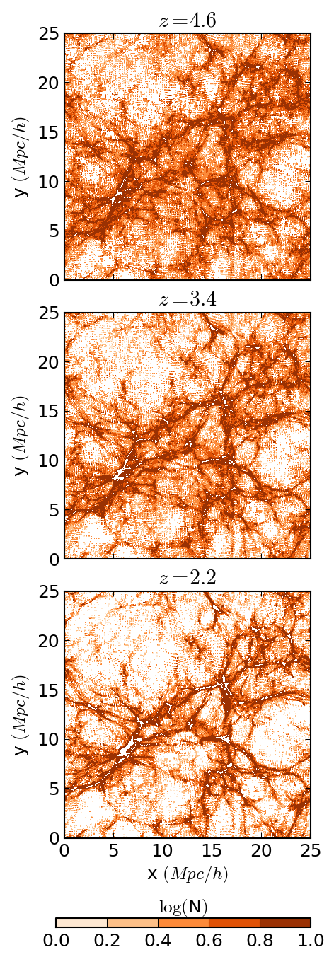
GADGET-3 follows a collisionless fluid with the standard -body method, and an ideal gas with smoothed particle hydrodynamics (SPH). The code solves simultaneously for the dynamics of the collisionless component and of the ideal gas, both subject to and coupled by gravity in an expanding background space. The -body implementation only differs from other cosmological codes by the accuracy of the gravitational field computation. A number of further physical processes have also been implemented in GADGET-3, from radiative cooling/heating physics to non-standard dark matter dynamics, star formation and feedback. In figure 3, we present the evolution of a filament with redshift and in figure 7 we show the image of a snapshot made with splotch 77 7 http://www.mpa-garching.mpg.de/~kdolag/Splotch. Such realizations can be used for visual confirmation before quantitative analysis as well as for public outreach and education.
Several optimization strategies have been added in GADGET-3. These include a Peano-Hilbert space decomposition, a massively parallel version of the Fast Fourier Transform library, the possibility of splitting the simulation data across several files (to facilitate and speed-up the input/output process), and the fact that the code can be run on an arbitrary number of processors. In its current version, GADGET-3 is highly efficient in memory consumption (it allocates up to bytes per particle) and communication bandwidth, is versatile and flexible, accurate and fast. Another important aspect is the scalability of the code, i.e. its performance when the number of processors is increased, which has currently been tested up to 16,000 cores.

We started all our simulations at with initial conditions based on second-order Lagrangian perturbation theory(Crocce et al., 2006), and adopted the same gravitational softening for the different species considered (i.e. gas, dark matter, stars), which however varies with the length of the box and the size of the mesh chosen. Specifically, we set the gravitational softening length to 0.8 kpc for the simulation having boxsize and resolution , while the softening is 3.25 kpc for the other two runs, i.e., the boxsize and resolution, and the boxsize and resolution. We used the ‘QUICKLYA’ routine in GADGET-3 to simulate the Lyman- forest, assuming the gas of primordial composition with a helium mass fraction of . We neglect metals and the evolution of elementary abundances, as well as feedback processes and galactic winds. Along the lines of Viel et al. (2010), we adopted a simplified criterion for star formation: all gas particles whose overdensity with respect to the mean is above 1000 and whose temperature is less than are turned into star particles immediately.
3.4 extract
The GADGET-3 snapshots contain various fields among which the position and velocity for both dark matter and gas particles. It also contains fields that are specific to the SPH treatment of gas particles: internal energy , density , electron fraction , hydrogen fraction and smoothing length . We use these fields to extract two samples:
- •
a particle sample: we extract a subsample of particles to study the temperature-density relation. For each particle the temperature is derived with the formula
(6) where . is the adiabatic index ( for monoatomic gas), is the mass of an hydrogen atom, is the Boltzmann constant and is the hydrogen fraction by mass. Figure 10 illustrates typical temperature-density diagrams obtained from this particle sample.
- •
a line of sight sample: following the traditional procedure in one-dimensional flux power studies (Gnedin and Hamilton, 2002; Croft et al., 2002), we extract lines of sight (LOS) from the simulation cube choosing random origin and axis. For each pixel of each LOS, we derive density , temperature , peculiar velocity and optical depth , all for H I only using the SPH equation:
(7) where is a scalar quantity, a position in the cube, the smoothing length, and a kernel function. The index runs on all particles. We use the 3D cubic spline kernel:
(8) where . These LOS are not mock spectra, in the sense that they do not match any properties (such as noise, resolution, metals absorption, …) of observational data. The quantity of particular interest for our study is the optical depth for H I, from which we compute the transmitted flux for each pixel.
3.5 Post-processing
The post-processing stage allows us to extract two categories of outputs. The first one is the large-box high-resolution power spectrum that is derived by an appropriate combination of the power spectra from 3 lower-resolution or smaller-box simulations, using the splicing technique described in section 5. At this stage, we fix the photo-ionization rate (or equivalently the UV flux) by requiring the effective optical depth at each redshift to follow the empirical power law , where and in agreement with observations (Meiksin, 2009). The rescaling coefficients, determined independently for each redshift bin using all the line-of-sight pixels, are typically between and . We perform this normalization a posteriori since it is computationally much cheaper than finding and fixing the appropriate photo-ionization rate a priori for each of the simulations. As explained in Theuns (2005), however, this is justified by the fact that when the gas is highly ionized and in photo-ionization equilibrium, as is the case for the Lyman- forest, the total heating rate per unit volume is independent of the amplitude of the UV flux. Gas dynamics can thus be considered not to be affected by the UV flux. The power spectrum is then computed from the scaled flux, and averaged over all lines of sight.
The second category results from the particle sample. It is used to derive the parameters and in the IGM. This is performed by estimating the location of the most populated region of the diagram using the mode of the 2D distribution, for particles lying in the region defined by and , with . Given the large tail of particles toward the high temperature regions where clusters of galaxies reside, in particular at low redshift, the mode was preferred to the mean since it is not affected by the precise choice of the bounds used to define the IGM. We estimate the mode by taking bins of and computing the barycenter of the five highest bins. A linear fit is then performed using these points.
4 Convergence tests
We base our minimal requirements for the resolution and box size of our simulations on the largest currently-available spectroscopic survey: SDSS-III/BOSS (Dawson et al., 2013). Those requirements are driven by the extension of the Lyman- forest that can be probed experimentally and by the measurement errors on the power spectrum , which set the convergence levels to be achieved in the simulations.
The quasar coadded spectra provided by the SDSS pipeline (Bolton et al., 2012) are computed with a constant pixel width of . The largest mode is bounded by the Nyquist-Shannon limit at . Instrumental constraints, however, make this theoretical limit very difficult to obtain with reasonable precision from data, and the largest mode measured in BOSS data by Palanque-Delabrouille et al. (2013a) is . The smallest mode is driven by the extension of the Lyman- forest which lies between the Lyman- and Lyman- emissions respectively at and . The exploitable Lyman- forest, however, is smaller than the separation of the two emission peaks due to their respective widths. Palanque-Delabrouille et al. (2013a) computed the 1D power spectrum from forest lengths corresponding to a third of the total available range in order to restrain the redshift span to at most. This led to . We therefore consider simulations that should cover the minimal range , which corresponds approximately to at .
In numerical simulations, the two relevant parameters are the size of the box that determines the smallest -mode (), and the ratio , where is number of particles, that drives the largest -mode. One may note that due to the computational algorithms used nowadays in simulations, such as smooth-particles hydrodynamics (SPH) or adaptive mesh refinement (AMR) in which “resolution follows density”, particle spacing in high-density regions will be significantly smaller than . Because the 1D power spectrum results from an integral over the 3D power spectrum up to (cf. Eq. 1), the resolution of the simulations has to be of the size of the smallest structures in the transverse direction. For structures in local hydrostatic equilibrium, this would be the Jeans scale, of order a few 100 kpc at . In an SPH approach, over-dense regions are sampled with much higher spatial resolution than average. Under-dense regions, on the other hand, might not necessarily be in local hydrostatic equilibrium. The decisive solution to ensure that the simulations do resolve the relevant structures is therefore to perform convergence tests.
The simulations used for the convergence test are all run with the same random seed and with the following cosmological parameters: . We ran two sets of simulations: the first set with simulations having the same box size of but changing the particle loading and therefore the mass resolution, the second with simulations having the same mass resolution but varying volumes, keeping fixed at . These two sets are listed in table 3 and the results at three different redshifts are presented in figures 4(a) and 4(b). Hereafter, we will use the notation (,) to represent a simulation with particles for each species (dark matter and baryons) in a box of size on a side.
| Mass-resolution test | Box-size test |
|---|---|
| (20,1024) | (120,1024) |
| (20,768) | (90,768) |
| (20,512) | (80,683) |
| (20,384) | (60,512) |
| (20,192) | (20,171) |


These convergence tests are more stringent than what has been done before, justified by our aim to use our simulation suite for comparison to data of higher quality. For instance, to probe the effect of the box size, Viel et al. (2004) compared to a reference simulation with and thus , and Bolton and Becker (2009) to a reference simulation i.e., . This is to be compared to our of 0.12. As regards the convergence on the mass-resolution, we explored a similar range of mass-resolutions as Bolton and Becker (2009) (in contrast, Viel et al. (2004) restricted to a minimum mass per particle 3 times larger), but using a box instead of .
The most difficult redshifts at which to achieve convergence are those at , since the mean flux level becomes very small at such epochs and under-dense regions, which are less well sampled than average in an SPH framework, are producing absorption. High redshift bins, however, are very important since gravitational collapse tends to suppress the differences in the linear-theory power spectra. These bins therefore highlight primordial differences between the matter power spectra resulting from different contributions of the various cosmological constituents. Some convergence problems can also arise at due to the fact that strong systems, which are very non-linear, might be simulated inadequately due to cosmic variance or lack of resolution. Low-redshift bins are also those where the measurements from QSO spectra have the smallest statistical error bars, making the convergence criteria tighter.
4.1 Mass resolution
We computed the ratio of the power spectra of each of the simulations listed in the first column of table 3 to the power spectrum of the (120,1024) simulation. The results presented in figure 4(a) show that an excess of power on large scales (small ) and a lack of power on small scales (large ) appear with decreasing resolution. As expected, this effect is stronger at higher redshift where the Lyman- forest probes low density regions, which are less well resolved in the SPH treatment since it is the mass (and not the spatial) resolution that is kept fixed. Further details about this effect can be found in Bolton and Becker (2009).
The dashed curves in figure 4(a) illustrate the level of the statistical uncertainties observed in the BOSS analysis (Palanque-Delabrouille et al., 2013a) at each redshift. At , the experimental uncertainties are larger than the maximum departure allowed on the plot and no longer appear.
Simulations with a mass resolution at least as good as for the (20,512) simulation all deviate by less than from the highest mass-resolution power spectrum over our minimal -range. This corresponds to a mean mass per particle of . Extending to , the (20,512) simulation deviates by at the largest redshift,.
4.2 Box size
The results of figure 4(b) show that the box size has an effect on all scales, and not only on the large scales that approach the Nyquist limit. This is due to the non-linear coupling of modes during gravitational evolution, and to the fact that even on scales close to the box size, mass-fluctuations are not fully linear.
As before, the dashed curves in figure 4(b) illustrate the level of the data uncertainties at each redshift. To reach , we see that we need a box size of at least . The most significant constraint comes from the largest scales that cannot be probed (or not with adequate precision) otherwise.
4.3 Summary of convergence requirements
In conclusion, the ideal simulation for our study should use a box and a mass resolution roughly equivalent to a (20,614) simulation, which translates into particles of each species. The mean mass of a gas particle is then .
Although convergence tests are specific to each problem and each statistical property for which convergence is sought, we can briefly compare to the results obtained by other studies. To infer the dark matter power spectrum from the Lyman- forest in high-resolution QSO absorption spectra covering , Viel et al. (2004) chose a simulation, i.e. a mass per gas particle of . To resolve the high redshift Lyman- forest in smoothed particle hydrodynamics simulations, a problem similar to our own, Bolton and Becker (2009) found that a box size of at least is preferable at all redshifts. They also found that while a mean gas particle mass is required at , a mass resolution at least 8 times better is needed at , i.e. . Our requirements are thus more stringent than selected in past, both in terms of box size and mass resolution.
Several tens of such simulations, as needed to compute our grid of cosmological simulations, would require several tens of millions of hours to be run, which is not an acceptable computational time. We address and solve this issue with the splicing technique presented in the next section.
5 Splicing
In the previous section we have estimated that simulating a flux power spectrum covering the range to ) with a unique simulation at sufficient precision for every redshift in the range requires particles of each species in a box of size . To obtain power spectra of equivalent resolution and box size in a reasonable computational time, we use the technique described in McDonald (2003). In this method, competing demands of large box size and high resolution are solved by splicing together the power spectra from pairs of large and small box simulations, using for the large-scale power, and for the small-scale power, both with . One must then correct the large box size simulation for the lack of resolution, and the small box size for the lack of non-linear coupling between the highest and the lowest -modes. The corrections are computed using a transition simulation that has same resolution as a and same box size as a .
One needs to distinguish three regimes when computing the full power spectra:
- •
, where is the minimum present in a box. The spliced flux power is the flux power of the simulation here taken as our reference, corrected for its low-resolution by a -independent factor evaluated at :
The possibility of using a constant factor for the largest -modes has been tested in McDonald (2003).
- •
, where is the Nyquist wave number of the large box. In this regime we use a similar correcting ratio, but taken at the wave number at which the flux power is calculated:
This is mathematically equivalent to considering the high-resolution simulation (25,768) as our reference, and correcting it for its small box size.
- •
. At these large -modes, the resolution correction is no longer a small factor. We thus take the simulation as our reference, and correct for its limited box size by a -independent factor evaluated at the fixed splicing point :
The splicing technique is applied for each redshift at which we compute the power spectrum. We illustrate the method and its accuracy on figure 5, using a set of smaller-resolution simulations to enhance the contrast between the different power spectra, as well as to allow the comparison to a full resolution run (labelled “exact” on the figure) with 1024 particles in a box. For this illustration, the large box-size, the large resolution and the transition simulations are (100,256), (25,256) and (25,64) simulations respectively. The spliced power spectrum obtained at is presented on the left of figure 5, along with the exact power spectrum and the individual runs entering the splicing estimate. The correction coefficient with respect to the reference power spectrum in each regime of -modes is shown on the right plot of figure 5. In the intermediate regime, the resolution correction increases towards smaller scales, reaching 40% for the set of simulations illustrated here. It shows less scale-dependence when taken as a box-size correction to the large-resolution power spectrum, but it is noisier since it requires taking the ratio of two simulations with different box sizes and thus different natural -modes. Although the correction factors show discontinuities at the boundary where the simulation chosen as reference changes, the spliced power spectrum is continuous by construction. In the large-mode splicing regime, at , it is unclear whether a constant box-size correction or even any correction at all is indeed the optimal combination, since both the correction factor and the residuals are at the same level of about 0.95. This regime, however, is only probed by the medium resolution SDSS-III/BOSS data in the highest redshift bins where measurement uncertainties significantly exceed the splicing errors. Its optimization is thus beyond the scope of this paper.
For the box size and resolution chosen for our simulation suite, the last regime begins at for , which is beyond the maximum mode that can be reached with BOSS or eBOSS data. The maximum correction factor, obtained for , is thus smaller than in the previous illustration. It ranges from 22% at to 5% at .
We estimate the accuracy of the technique from the splicing residuals, defined as the ratio of the spliced to the exact power spectrum. The splicing residuals show no dependence with redshift. The residuals at are overlaid on the right plot of figure 5. In figure 6, they are plotted for and , along with the statistical uncertainty at the same redshifts obtained in the most recent BOSS analysis (Palanque-Delabrouille et al., 2013a). Over the -range of interest for BOSS data, the residuals have an average of with an of 0.01. The largest excess is seen near . A simulation with a larger box size would be needed to reduce the splicing residuals further. For the purpose of this study, the splicing technique is accurate at the 2% level over the entire -range of interest.
6 Results and discussions
Several checks were performed to validate our simulations. We first verified that the power spectrum of independent simulations obtained either with different cosmological parameters or different seeds is consistent with the power spectrum derived from the Taylor expansion of Sec. 2. We then present a comparison of our central model with the one-dimensional Lyman- forest power spectrum obtained with BOSS by Palanque-Delabrouille et al. (2013a). This allows us to quantify the agreement between our simulation and the measured power spectrum. Finally, we discuss some characteristics of our simulations. In particular, we describe the effect on the flux power spectrum of some of the parameters we have varied, and we show the diagrams from which we derive the two parameters and that describe the IGM.
6.1 Assessment checks
We performed three categories of assessment checks. The first one verifies the statistical errors in the simulation relative to the number of lines of sight used to compute the one-dimensional power spectrum. The second one assesses the accuracy of our second-order Taylor expansion to model the power spectrum by comparing its prediction to the simulated power spectrum for simulations other than those used in the grid. The last category tests the impact of cosmic variance from the use of a given random seed.
For each simulation, the one-dimensional power spectrum was computed from 100.000 lines of sight. This large number is necessary to ensure that the simulation uncertainties remain about an order of magnitude smaller than current most precise data measurements (taken from (Palanque-Delabrouille et al., 2013b)). We ensured that the simulation uncertainties were not artificially limited by an oversampling of the simulated volume: this was done by considering different numbers of lines of sight (from 5.000 to 100.000). For each redshift and mode, the power spectrum value is taken as the mean over the lines of sight and the uncertainty on the mean as the of the distribution divided by . We checked that the uncertainty on each point of the power spectrum scaled as the square-root of the number of lines of sight used to compute it, at better than the percent level.
To test the accuracy with which our Taylor expansion reproduces the power spectrum for different cosmologies, we performed simulations with input cosmological and astrophysical parameters different from those that were used to compute the derivatives. We tested the most relevant parameters for our study. One simulation was run with different and , two others with different and , and a last set with all input parameters different from their values in the grid simulations. In each case, we computed the power spectra corresponding to the twelve redshift bins in the range . We then performed a simple fit of the six parameters (, , , , AMPL, GRAD) using our second-order Taylor expansion as model.
The results are summarized in Tab. 4. The last column shows the fitted values over 100.000 lines of sight. The uncertainty is estimated as the of the distribution for each parameter fitted over 10 subsamples of 10.000 lines of sight each, divided by . The configurations were chosen so as to probe different relevant regions of the parameter phase space. These tests give results in excellent agreement with the input parameters. The level of accuracy achieved with these validation tests is 3 to 5 times better than the errors we expect on these parameters from a fit to data given the uncertainties of Palanque-Delabrouille et al. (2013a). We note that the accuracy drops rapidly, however, as we test values outside the range that was used to compute the derivatives (cf. table 2), as indicated by the almost discrepancy on the fitted value of in the last test. Since our variation range was purposely chosen to be wide enough to include all recent results, this is not expected to cause any problem in the future. These checks thus demonstrate that our Taylor expansion adequately models the power spectrum for any set of input parameters within the range of table 2.
| Test configuration | Parameter | Input value | Fitted value |
|---|---|---|---|
| . | |||
| . | |||
| . | |||
| . | |||
| . | |||
| . | |||
| . | |||
| . | |||
| . | |||
| . | |||
| . | |||
| . | |||
| . | |||
| . | |||
| . | |||
| . | |||
| . | |||
| . | |||
| All parameters | . | ||
| . | |||
| . | |||
| . | |||
| . | |||
| . | |||
| All parameters | . | ||
| . | |||
| . | |||
| . | |||
| . | |||
| . |
Finally, we produced a new simulation with the same parameters as our central simulation but using a different random seed to compute the initial conditions. Snapshots of the resulting gas distribution in the two cases are shown in figure 7. The derived power spectra for the two seeds are in excellent agreement on low scales. On the largest scales, the two power spectra can differ by up to 2 to 3 at all redshifts, indicating a sample variance contribution to the uncertainty on the simulated power spectrum due to the fact that the simulation box has a size close to the largest modes measured. We again performed a simple fit on the power spectrum measured with the new seed using our Taylor expansion as model. The results are given in table 5. They show that cosmic variance has an impact on the power spectrum that exceeds the simulation statistical uncertainty and will therefore need to be included as a systematic uncertainty when comparing our model to data.


| Parameter | Input value | Fitted value |
|---|---|---|
| . | ||
| . | ||
| . | ||
| . | 65 | |
| . | ||
| . |
6.2 Comparison to SDSS-III/BOSS DR9 data
In Palanque-Delabrouille et al. (2013a), the one-dimensional Lyman- forest power spectrum is measured with 13,821 quasar spectra from SDSS-III/BOSS DR9 selected on the basis of their high quality, large signal-to-noise ratio, and good spectral resolution. The power spectra are measured over twelve redshift bins from to , and scales from 0.001 to (see figure 8).
In order to compare the measurements to the power spectrum obtained for our central model model, we normalized the simulation power spectrum at each redshift by constraining the effective optical depth to follow the power law evolution , where and . To account for the effect of the correlated Si iii absorption, we correct the simulated power spectrum by a multiplicative term, with following the suggestion of McDonald et al. (2006). The parameter is adjusted and is fixed at 2271 km/s. We model the imperfection of the resolution of BOSS spectra though a multiplicative term. Finally, we allow for imperfection in the noise estimate of the BOSS spectra with eight additive terms (one for each redshift bin).
Figure 8 illustrates the good agreement between the data and the simulations. Without any adjustment of the cosmological and astrophysical parameters, the per number of degrees of freedom is already better than 1.2. The good agreement between data and simulation covers the whole redshift range, , in contrast with the cosmological analysis described in Palanque-Delabrouille et al. (2013a) which was performed over the reduced redshift range . This simple comparison demonstrates the improvement obtained with these simulations over the previous generation of simulations (Viel et al., 2010).
6.3 Power spectrum
Figure 9 illustrates the impact on the power spectrum of our four cosmological parameters. We compare the power spectrum computed from our best-guess model to the one obtained when varying each parameter, one at a time. We note that the dependence on the value of the four parameters is as expected according to their physical meaning. We briefly explain the different behaviors below.
The spectral index represents the evolution of the primordial density fluctuations with respect to through . A larger therefore increases the power at large , as seen in the top left panel of figure 9.
The parameter measures the amplitude of the linear matter density fluctuations today in spheres of size , and thus determines the normalization of the matter power spectrum. To first order, increasing the value of therefore increases the power spectrum on all scales, as shown in the top right panel of figure 9. A slightly larger effect, however, is seen on large scales, since an excess in the amplitude of the fluctuations will favor the merging of small scale fluctuations, thus enhancing the power on larger scales. This tiny trend is purely non-linear and not expected in the evolution with of the linear power-spectrum.
The present-day Hubble constant (in units of velocity/distance) allows the conversion from distance-space to -space (units of inverse velocity). Therefore, if is increased, a given distance will correspond to a higher , thus leading to an increase of power since the power spectrum, which is a decreasing function of , is shifted to the right. This is indeed what is observed in the lower left panel of figure 9.
Finally, the parameter quantifies the fraction of matter density in a flat Universe. Because and the dark energy density vary in opposite directions, a higher delays the onset of dark energy domination, thus increasing the time available for structure formation. In addition, in a larger universe, more structures (in particular small ones that would not collapse otherwise) will be formed, leading to an increase of the power spectrum, especially at high . This is in agreement with the plots in the lower right panel of figure 9.

6.4 Density-temperature relation
In figure 10, we present the diagrams obtained from our central simulation at each of the snapshot redshifts. We can distinguish three different populations – the IGM, the stars, and the clusters – with a clear evolution with redshift for each of them.
The IGM is described by the low density and low temperature particles. This is the regime that dominates at high redshift. At later times, however, fewer and fewer particles reside in this part of the diagram, since they are captured by collapsing over-densities. We use this region to extract the and parameters, displayed in figure 11, where they are compared to the measurements of Becker et al. (2011).
The particles with higher temperature correspond to clusters and galactic gas. As expected, their density increases as structures are formed in the simulation box. They therefore become more prominent at lower redshifts.
In our simulations dedicated to the study of the IGM though the Lyman- forest measurements, star formation undergoes a simplified treatment, which reflects as the sharp cut-off at . Any particle sufficiently dense and cool is transformed into a star particle. The latter is used for gravity force calculation, but does not undergo SPH treatment like baryonic gas does.


7 Conclusions
We have designed and produced a grid of cosmological simulations, which may be used to extract constraints on cosmological parameters from Lyman- surveys, whether current like SDSS-III/BOSS or future like SDSS-IV/eBOSS. These simulations cover the redshift range . They explore the cosmological parameters , , , and over a large range centered on Planck measurements, as well as the astrophysical parameters and in a range covering most recent results.
Using the splicing technique of McDonald (2003), we computed 1D power spectra from simulations equivalent to a box filled with particles of each species (here dark matter and baryonic gas), abbreviated to (100, 3072) using our standard notation, from lower-resolution (100,768) and smaller box-size (25,768) simulations, combined using a transition (25,192) simulation. We show that the splicing technique allows us to approximate the exact full-resolution large-box simulation with an accuracy at the 2% level.
While one full-size high-resolution (100,3072) simulation would have required of order one million hours, one equivalent set of 3 simulations consumes an average of 70,000 hours of CPU time, with most of the time in the simulation pipeline (see figure 2) being spent on performing the hydrodynamical simulations. The data volume produced by each set is 1.6 terabytes. Therefore, the whole grid represents about 2 millions hours of CPU time and a volume of 45 terabytes of data.
From the 1D power-spectra that we computed at each point of the grid, we derived a second-order Taylor expansion around our best-guess model. It describes the evolution of the 1D power spectrum with changes in either the cosmological or the astrophysical parameters that we studied. We have performed several check runs to ensure the quality and validity of our simulation grid, using either different seeds, or off-the-grid values of the cosmological and astrophysical parameters. These checks were all consistent with the power spectrum predicted using our second-order Taylor expansion, thus validating it. We compared our central simulation to published data from BOSS and showed that they were already in good agreement without any adjustment of any of the simulation parameters. In forthcoming work, we will use this Taylor expansion for a quantitative comparison to data in order to extract best-fit cosmological parameters.
These simulations are accompanied by a set of simulations where massive neutrinos are included. These required additional developments for an efficient treatment and a proper account of the additional particles (at all levels of the pipeline: in CAMB, in the setup of the initial conditions for thermal velocities, in Gadget-3, etc.), but are otherwise produced with a pipeline similar to the one presented in this study. The details about the simulations with massive neutrinos can be found in the companion paper (Rossi et al., 2014). Additional parameters can yet be included in the same context. However, due to the presence of the cross terms that are necessary for an accurate modeling of the likelihood function that illustrates the variation of the power spectrum in all directions of this growing parameter-space, adding new parameters will become more and more expensive in terms of calculation time.
Appendix A List of all simulations
We summarize in table 6 and 7 all the simulations mentioned in the paper. For box size and number of particles, refers to a simulation with particles per species (gas or dark matter, thus particles total) in a box of size on a side. Standard parameters are . Unless parameter names are explicitly listed, values are given for all parameters in the order just mentioned. All parameters are assumed to have their standard value unless specified otherwise. Except for the simulations performed for the convergence tests or to compute the exact power spectrum in the splicing test, all simulations are using the splicing technique to combine each set of three simulations into a single one of equivalent size to the largest box and equivalent mass-resolution to the best mass resolution. In the first column of the table 6, and indicate simulations needed to compute the first and second order derivatives with respect to parameter , and indicate additional simulations required to compute cross-derivatives with respect to parameters and , where and are explicitly given in the same column. In the last column of the same table, we also give the values of the shape parameter and of where corresponds to the pivot redshift of Ly power spectrum measurements in Palanque-Delabrouille et al. (2013a) and McDonald (2003). These parameters are not used in this work but we make them available since they are closely related to observations and were often used in the pioneering work on Ly forest measurements.
| Grid | |||
| Type | Box size, particles | Simulation parameters | ; |
| Central | (25,768)+(100,768)+(25,192) | Standard | 0.26; 0.21 |
| , | (25,768)+(100,768)+(25,192) | 0.26; 0.21 | |
| , | (25,768)+(100,768)+(25,192) | 0.26; 0.21 | |
| , | (25,768)+(100,768)+(25,192) | 0.25; 0.21 | |
| , | (25,768)+(100,768)+(25,192) | 0.28; 0.21 | |
| , | (25,768)+(100,768)+(25,192) | 0.27; 0.18 | |
| , | (25,768)+(100,768)+(25,192) | 0.25; 0.24 | |
| , | (25,768)+(100,768)+(25,192) | 0.26; 0.19 | |
| , | (25,768)+(100,768)+(25,192) | 0.26; 0.22 | |
| , | (25,768)+(100,768)+(25,192) | 0.26; 0.21 | |
| , | (25,768)+(100,768)+(25,192) | 0.26; 0.21 | |
| , | (25,768)+(100,768)+(25,192) | 0.26; 0.21 | |
| , | (25,768)+(100,768)+(25,192) | 0.26; 0.21 | |
| (25,768)+(100,768)+(25,192) | , | 0.28; 0.21 | |
| (25,768)+(100,768)+(25,192) | , | 0.25; 0.24 | |
| (25,768)+(100,768)+(25,192) | , | 0.26; 0.22 | |
| (25,768)+(100,768)+(25,192) | , | 0.26; 0.21 | |
| (25,768)+(100,768)+(25,192) | , | 0.26; 0.21 | |
| (25,768)+(100,768)+(25,192) | , | 0.27; 0.24 | |
| (25,768)+(100,768)+(25,192) | , | 0.28; 0.22 | |
| (25,768)+(100,768)+(25,192) | , | 0.28; 0.21 | |
| (25,768)+(100,768)+(25,192) | , | 0.28; 0.21 | |
| (25,768)+(100,768)+(25,192) | , | 0.25; 0.26 | |
| (25,768)+(100,768)+(25,192) | , | 0.25; 0.24 | |
| (25,768)+(100,768)+(25,192) | , | 0.25; 0.24 | |
| (25,768)+(100,768)+(25,192) | , | 0.26; 0.22 | |
| (25,768)+(100,768)+(25,192) | , | 0.26; 0.22 | |
| (25,768)+(100,768)+(25,192) | , | 0.26; 0.21 | |
| Convergence tests | ||
| Type | Box size, particles | Simulation parameters |
| Resolution | (20,1024) | Standard |
| Resolution | (20,768) | Standard |
| Resolution | (20,512) | Standard |
| Resolution | (20,384) | Standard |
| Resolution | (20,192) | Standard |
| Box size | (120,1024) | Standard |
| Box size | (90,768) | Standard |
| Box size | (80,683) | Standard |
| Box size | (60,512) | Standard |
| Box size | (20,171) | Standard |
| Splicing tests | ||
| Type | Box size, particles | Simulation parameters |
| Grid-like | (25,256)+(100,256)+(25,64) | Standard |
| Exact | (100,1024) | Standard |
| Validity checks | ||
| Type | Box size, particles | Simulation parameters |
| Random seed | (25,768)+(100,768)+(25,192) | Standard |
| Off-grid 1 | (25,768)+(100,768)+(25,192) | |
| Off-grid 2 | (25,768)+(100,768)+(25,192) | |
| Off-grid 3 | (25,768)+(100,768)+(25,192) | |
| Off-grid 4 | (25,768)+(100,768)+(25,192) | |
| Off-grid 5 | (25,768)+(100,768)+(25,192) | |
Acknowledgements.
We acknowledge PRACE (Partnership for Advanced Computing in Europe) for awarding us access to resource curie-thin nodes based in France at TGCC, under allocation number 2012071264.This work was also granted access to the resources of CCRT under the allocation 2013-t2013047004 made by GENCI (Grand Equipement National de Calcul Intensif).
A.B., N.P.-D., G.R. and Ch.Y. acknowledge support from grant ANR-11-JS04-011-01 of Agence Nationale de la Recherche.
M.V. is supported by ERC-StG ”CosmoIGM”.
JSB acknowledges the support of a Royal Society University Research Fellowship.
We thank Volker Springel for making GADGET-3 available to our team.
References
- Palanque-Delabrouille et al. (2013a) Palanque-Delabrouille, N., C. Yèche, A. Borde, et al. The one-dimensional Ly-alpha forest power spectrum from BOSS. Astronomy & Astrophysics, 559:A85, 2013a. arXiv:1306.5896.
- Lynds (1971) Lynds, R. The Absorption-Line Spectrum of 4c 05.34. The Astrophysical Journal, 164:L73, 1971.
- Bi et al. (1992) Bi, H. G., G. Boerner, and Y. Chu. An alternative model for the Ly-alpha absorption forest. Astronomy & Astrophysics, 266:1–5, 1992.
- Miralda-Escude and Rees (1993) Miralda-Escude, J. and M. J. Rees. Tests for the minihalo model of the Lyman-alpha forest. Monthly Notices of the Royal Astronomical Society, 260:617–624, 1993.
- Croft et al. (1998) Croft, R. A. C., D. H. Weinberg, N. Katz, et al. Recovery of the Power Spectrum of Mass Fluctuations from Observations of the Ly-alpha Forest. The Astrophysical Journal, 495:44–62, 1998. arXiv:astro-ph/9708018.
- Cen (1992) Cen, R. A hydrodynamic approach to cosmology - Methodology. The Astrophysical Journal Supplement Series, 78:341, 1992.
- Zhang et al. (1995) Zhang, Y., P. Anninos, and M. L. Norman. A Multispecies Model for Hydrogen and Helium Absorbers in Lyman-Alpha Forest Clouds. The Astrophysical Journal, 453, 1995. arXiv:astro-ph/9508133.
- Hernquist et al. (1996) Hernquist, L., N. Katz, D. H. Weinberg, et al. The Lyman-Alpha Forest in the Cold Dark Matter Model. The Astrophysical Journal, 457:1–11, 1996. arXiv:astro-ph/9509105.
- Hui and Gnedin (1997) Hui, L. and N. Y. Gnedin. Equation of state of the photoionized intergalactic medium. Monthly Notices of the Royal Astronomical Society, 292:27–42, 1997. arXiv:astro-ph/9612232.
- Hui et al. (1997) Hui, L., N. Y. Gnedin, and Y. Zhang. The Statistics of Density Peaks and the Column Density Distribution of the Ly-alpha Forest. The Astrophysical Journal, 486:599–622, 1997. arXiv:astro-ph/9608157.
- Viel et al. (2004) Viel, M., M. G. Haehnelt, and V. Springel. Inferring the dark matter power spectrum from the Lyman alpha forest in high-resolution QSO absorption spectra. Monthly Notices of the Royal Astronomical Society, 354:684–694, 2004. arXiv:astro-ph/0404600.
- Gnedin (1998) Gnedin, N. Y. Probing the Universe with the Ly-alpha forest - II. The column density distribution. Monthly Notices of the Royal Astronomical Society, 299:392–402, 1998. arXiv:astro-ph/9706286.
- Hui et al. (1999) Hui, L., A. Stebbins, and S. Burles. A Geometrical Test of the Cosmological Energy Contents Using the Ly-alpha Forest. The Astrophysical Journal, 511:L5–L8, 1999. arXiv:astro-ph/9807190.
- Gaztanaga and Croft (1999) Gaztanaga, E. and R. A. C. Croft. Predictions for the clustering properties of the Lyman-alpha forest – I. One-point statistics. Monthly Notices of the Royal Astronomical Society, 309:885–904, 1999. arXiv:astro-ph/9811480.
- Nusser and Haehnelt (1999) Nusser, A. and M. Haehnelt. A first step towards a direct inversion of the Lyman forest in QSO spectra. Monthly Notices of the Royal Astronomical Society, 303:179–187, 1999. arXiv:astro-ph/9806109.
- Feng and Fang (2000) Feng, L.-l. and L.-z. Fang. Non-Gaussianity and the Recovery of the Mass Power Spectrum from the Ly-alpha Forest. The Astrophysical Journal, 535:519–529, 2000. arXiv:astro-ph/0001348.
- McDonald et al. (2000) McDonald, P., J. Miralda-Escude, M. Rauch, et al. The Observed Probability Distribution Function, Power Spectrum, and Correlation Function of the Transmitted Flux in the Ly-alpha Forest. The Astrophysical Journal, 543:1–23, 2000. arXiv:astro-ph/9911196.
- Hui et al. (2001) Hui, L., S. Burles, U. Seljak, et al. On Estimating the QSO Transmission Power Spectrum. The Astrophysical Journal, 552:15–35, 2001. arXiv:astro-ph/0005049.
- Alcock and Paczyński (1979) Alcock, C. and B. Paczyński. An evolution free test for non-zero cosmological constant. Nature, 281:358–359, 1979.
- McDonald and Miralda-Escude (1999) McDonald, P. and J. Miralda-Escude. Measuring the Cosmological Geometry from the Ly-alpha Forest along Parallel Lines of Sight. The Astrophysical Journal, 518:24–31, 1999. arXiv:astro-ph/9807137.
- Croft et al. (2002) Croft, R. A. C., D. H. Weinberg, M. Bolte, et al. Toward a Precise Measurement of Matter Clustering: Ly-alpha Forest Data at Redshifts 2–4. The Astrophysical Journal, 581:20–52, 2002. arXiv:astro-ph/0012324.
- McDonald and Eisenstein (2007) McDonald, P. and D. Eisenstein. Dark energy and curvature from a future baryonic acoustic oscillation survey using the Lyman-alpha forest. Physical Review D, 76:063009, 2007. arXiv:astro-ph/0607122.
- Seljak et al. (2005) Seljak, U., A. Makarov, P. McDonald, et al. Cosmological parameter analysis including SDSS Ly-alpha forest and galaxy bias: Constraints on the primordial spectrum of fluctuations, neutrino mass, and dark energy. Physical Review D, 71:103515, 2005. arXiv:astro-ph/0407372.
- Viel et al. (2010) Viel, M., M. G. Haehnelt, and V. Springel. The effect of neutrinos on the matter distribution as probed by the intergalactic medium. Journal of Cosmology and Astroparticle Physics, 2010:015–015, 2010. arXiv:1003.2422.
- Croft et al. (1999) Croft, R. A. C., D. H. Weinberg, M. Pettini, et al. The Power Spectrum of Mass Fluctuations Measured from the Ly-alpha Forest at Redshift z = 2.5. The Astrophysical Journal, 520:1–23, 1999. arXiv:astro-ph/9809401.
- Kim et al. (2004a) Kim, T.-S., M. Viel, M. G. Haehnelt, et al. Erratum: The power spectrum of the flux distribution in the Lyman-alpha forest of a large sample of UVES QSO Absorption Spectra (LUQAS). Monthly Notices of the Royal Astronomical Society, 351:1471–1472, 2004a.
- Kim et al. (2004b) Kim, T. S., M. Viel, M. G. Haehnelt, et al. The power spectrum of the flux distribution in the Lyman-alpha forest of a large sample of UVES QSO absorption spectra (LUQAS). Monthly Notices of the Royal Astronomical Society, 347:355–366, 2004b. arXiv:astro-ph/0308103.
- York et al. (2000) York, D. G., J. Adelman, J. E. Anderson, Jr., et al. The Sloan Digital Sky Survey: Technical Summary. The Astronomical Journal, 120:1579–1587, 2000. arXiv:astro-ph/0006396.
- McDonald et al. (2006) McDonald, P., U. Seljak, S. Burles, et al. The Ly-alpha Forest Power Spectrum from the Sloan Digital Sky Survey. The Astrophysical Journal Supplement Series, 163:80–109, 2006. arXiv:astro-ph/0405013.
- McDonald et al. (2005) McDonald, P., U. Seljak, R. Cen, et al. The Linear Theory Power Spectrum from the Ly-alpha Forest in the Sloan Digital Sky Survey. The Astrophysical Journal, 635:761–783, 2005. arXiv:astro-ph/0407377.
- Eisenstein et al. (2011) Eisenstein, D. J., D. H. Weinberg, E. Agol, et al. SDSS-III: Massive Spectroscopic Surveys of the Distant Universe, the Milky Way and Extra-Solar Planetary Systems. The Astronomical Journal, 142:72, 2011. arXiv:1101.1529v1.
- Dawson et al. (2013) Dawson, K. S., D. J. Schlegel, C. P. Ahn, et al. The Baryon Oscillation Spectroscopic Survey of SDSS-III. The Astronomical Journal, 145:10, 2013. arXiv:1208.0022.
- Pâris et al. (2012) Pâris, I., P. Petitjean, E. Aubourg, et al. The Sloan Digital Sky Survey quasar catalog: ninth data release. Astronomy & Astrophysics, 548:A66, 2012. arXiv:1210.5166.
- Lee et al. (2013a) Lee, K.-g., S. Bailey, L. E. Bartsch, et al. The BOSS Ly-alpha forest sample from SDSS data release 9. The Astronomical Journal, 145:69, 2013a. arXiv:1211.5146.
- Ahn et al. (2012) Ahn, C. P., R. Alexandroff, C. Allende Prieto, et al. The Ninth Data Release of the Sloan Digital Sky Survey: First Spectroscopic Data from the SDSS-III Baryon Oscillation Spectroscopic Survey. The Astrophysical Journal Supplement Series, 203:21, 2012. arXiv:1207.7137.
- Busca et al. (2013) Busca, N. G., T. Delubac, J. Rich, et al. Baryon acoustic oscillations in the Ly-alpha forest of BOSS quasars. Astronomy & Astrophysics, 552:A96, 2013. arXiv:1211.2616.
- Slosar et al. (2013) Slosar, A., V. Iršič, D. Kirkby, et al. Measurement of baryon acoustic oscillations in the Lyman-alpha forest fluctuations in BOSS data release 9. Journal of Cosmology and Astroparticle Physics, 2013:026–026, 2013. arXiv:1301.3459.
- Kirkby et al. (2013) Kirkby, D., D. Margala, A. Slosar, et al. Fitting methods for baryon acoustic oscillations in the Lyman-alpha forest fluctuations in BOSS data release 9. Journal of Cosmology and Astroparticle Physics, 2013:024–024, 2013. arXiv:1301.3456.
- Lee et al. (2013b) Lee, K.-g., J. F. Hennawi, M. White, et al. Observational Requirements for Lyman-alpha Forest Tomographic Mapping of Large-Scale Structure at z 2. 2013b. arXiv:1309.1477.
- Viel and Haehnelt (2006) Viel, M. and M. G. Haehnelt. Cosmological and astrophysical parameters from the Sloan Digital Sky Survey flux power spectrum and hydrodynamical simulations of the Lyman alpha forest. Monthly Notices of the Royal Astronomical Society, 365:231–244, 2006. arXiv:astro-ph/0508177.
- Bolton et al. (2008) Bolton, J. S., M. Viel, T.-S. Kim, et al. Possible evidence for an inverted temperature–density relation in the intergalactic medium from the flux distribution of the Ly-alpha forest. Monthly Notices of the Royal Astronomical Society, 386:1131–1144, 2008. arXiv:0711.2064.
- Bird et al. (2011) Bird, S., H. V. Peiris, M. Viel, et al. Minimally parametric power spectrum reconstruction from the Lyman-alpha forest. Monthly Notices of the Royal Astronomical Society, 413:1717–1728, 2011. arXiv:1010.1519.
- Bird et al. (2012) Bird, S., M. Viel, and M. G. Haehnelt. Massive neutrinos and the non-linear matter power spectrum. Monthly Notices of the Royal Astronomical Society, 420:2551–2561, 2012. arXiv:1109.4416.
- Springel (2005) Springel, V. The cosmological simulation code GADGET-2. Monthly Notices of the Royal Astronomical Society, 364:1105–1134, 2005. arXiv:astro-ph/0505010.
- Schlegel et al. (2011) Schlegel, D., F. Abdalla, T. Abraham, et al. The BigBOSS Experiment. 2011. arXiv:1106.1706.
- Tang (1993) Tang, B. Orthogonal Array-Based Latin Hypercubes. Journal of the American Statistical Association, 88:1392–1397, 1993.
- McKay et al. (2000) McKay, M. D., R. J. Beckman, and W. J. Conover. A Comparison of Three Methods for Selecting Values of Input Variables in the Analysis of Output From a Computer Code. Technometrics, 42:55–61, 2000.
- Heitmann et al. (2009) Heitmann, K., D. Higdon, M. White, et al. The Coyote Universe. II. Cosmological Models and Precision Emulation of the Nonlinear Matter Power Spectrum. The Astrophysical Journal, 705:156–174, 2009. arXiv:0902.0429.
- Schneider et al. (2011) Schneider, M. D., S. Cole, C. S. Frenk, et al. Fast Generation of Ensembles of Cosmological N-Body Simulations via Mode Resampling. The Astrophysical Journal, 737:11, 2011. arXiv:1103.2767.
- Viel et al. (2006) Viel, M., M. G. Haehnelt, and A. Lewis. The Lyman alpha forest and WMAP year three. Monthly Notices of the Royal Astronomical Society: Letters, 370:L51–L55, 2006. arXiv:astro-ph/0604310.
- Wang et al. (2013) Wang, M.-y., R. A. C. Croft, A. H. G. Peter, et al. Lyman-alpha Forest Constraints on Decaying Dark Matter. 2013. arXiv:1309.7354.
- Planck Collaboration et al. (2013) Planck Collaboration, P. A. R. Ade, N. Aghanim, et al. Planck 2013 results. XVI. Cosmological parameters. 2013. arXiv:1303.5076.
- Komatsu et al. (2011) Komatsu, E., K. M. Smith, J. Dunkley, et al. Seven-Year Wilkinson Microwave Anisotropy Probe (WMAP) Observations: Cosmological Interpretation. The Astrophysical Journal Supplement Series, 192:18, 2011. arXiv:1001.4538.
- Hou et al. (2014) Hou, Z., C. L. Reichardt, K. T. Story, et al. Constraints on Cosmology from the Cosmic Microwave Background Power Spectrum of the 2500 deg2 SPT-SZ Survey. The Astrophysical Journal, 782:74, 2014. arXiv:1212.6267.
- Conley et al. (2011) Conley, A., J. Guy, M. Sullivan, et al. Supernova Constraints and Systematic Uncertainties from the First Three Years of the Supernova Legacy Survey. The Astrophysical Journal Supplement Series, 192:1, 2011. arXiv:1104.1443.
- Sullivan et al. (2011) Sullivan, M., J. Guy, A. Conley, et al. SNLS3: Constraints on Dark Energy Combining the Supernova Legacy Survey Three-Year Data with Other Probes. The Astrophysical Journal, 737:102, 2011. arXiv:arXiv:1104.1444v2.
- Becker et al. (2011) Becker, G. D., J. S. Bolton, M. G. Haehnelt, et al. Detection of extended HeII reionization in the temperature evolution of the intergalactic medium. Monthly Notices of the Royal Astronomical Society, 410:1096–1112, 2011. arXiv:1008.2622.
- Garzilli et al. (2012) Garzilli, A., J. S. Bolton, T.-S. Kim, et al. The intergalactic medium thermal history at redshift z = 1.7-3.2 from the Ly forest: a comparison of measurements using wavelets and the flux distribution. Monthly Notices of the Royal Astronomical Society, 424:1723–1736, 2012. arXiv:1202.3577.
- Lidz et al. (2010) Lidz, A., C.-A. Faucher-Giguère, A. Dall’Aglio, et al. A Measurement of Small-Scale Structure in the 2.2 z 4.2 Ly-alpha Forest. The Astrophysical Journal, 718:199–230, 2010. arXiv:0909.5210.
- Schaye et al. (2000) Schaye, J., T. Theuns, M. Rauch, et al. The thermal history of the intergalactic medium. Monthly Notices of the Royal Astronomical Society, 318:817–826, 2000. arXiv:astro-ph/9912432.
- Gnedin and Hui (1998) Gnedin, N. Y. and L. Hui. Probing the Universe with the Lyalpha forest - I. Hydrodynamics of the low-density intergalactic medium. Monthly Notices of the Royal Astronomical Society, 296:44–55, 1998. astro-ph/9706219.
- Theuns et al. (2002) Theuns, T., M. Viel, S. Kay, et al. Galactic Winds in the Intergalactic Medium. The Astrophysical Journal, 578:L5–L8, 2002. astro-ph/0208418.
- McQuinn et al. (2011) McQuinn, M., L. Hernquist, A. Lidz, et al. The signatures of large-scale temperature and intensity fluctuations in the Lyman forest. Monthly Notices of the Royal Astronomical Society, 415:977–992, 2011. arXiv:astro-ph.CO/1010.5250.
- McDonald et al. (2005) McDonald, P., U. Seljak, R. Cen, et al. Physical effects on the Ly forest flux power spectrum: damping wings, ionizing radiation fluctuations and galactic winds. Monthly Notices of the Royal Astronomical Society, 360:1471–1482, 2005. astro-ph/0407378.
- Palanque-Delabrouille et al. (2013b) Palanque-Delabrouille, N., C. Magneville, C. Yèche, et al. Luminosity function from dedicated SDSS-III and MMT data of quasars in 0.7 z 4.0 selected with a new approach. Astronomy & Astrophysics, 551:A29, 2013b. arXiv:1209.3968.
- Lewis et al. (2000) Lewis, A., A. Challinor, and A. Lasenby. Efficient Computation of Cosmic Microwave Background Anisotropies in Closed Friedmann-Robertson-Walker Models. The Astrophysical Journal, 538:473–476, 2000. arXiv:astro-ph/9911177.
- Seljak and Zaldarriaga (1996) Seljak, U. and M. Zaldarriaga. A Line-of-Sight Integration Approach to Cosmic Microwave Background Anisotropies. The Astrophysical Journal, 469:437, 1996. arXiv:astro-ph/9603033.
- Bertschinger (1995) Bertschinger, E. COSMICS: Cosmological Initial Conditions and Microwave Anisotropy Codes. 1995. arXiv:astro-ph/9506070.
- Crocce et al. (2006) Crocce, M., S. Pueblas, and R. Scoccimarro. Transients from initial conditions in cosmological simulations. Monthly Notices of the Royal Astronomical Society, 373:369–381, 2006. arXiv:astro-ph/0606505.
- Rossi et al. (2014) Rossi, G., N. Palanque-Delabrouille, A. Borde, et al. A Suite of Hydrodynamical Simulations for the Lyman-Alpha Forest with Massive Neutrinos. 2014. arXiv:1401.6464.
- Ali-Haimoud and Bird (2012) Ali-Haimoud, Y. and S. Bird. An efficient implementation of massive neutrinos in non-linear structure formation simulations. Monthly Notices of the Royal Astronomical Society, 428:3375–3389, 2012. arXiv:1209.0461.
- Springel et al. (2001) Springel, V., N. Yoshida, and S. D. White. GADGET: a code for collisionless and gasdynamical cosmological simulations. New Astronomy, 6:79–117, 2001. arXiv:astro-ph/0003162.
- Gnedin and Hamilton (2002) Gnedin, N. Y. and A. J. S. Hamilton. Matter power spectrum from the Lyman-alpha forest: myth or reality? Monthly Notices of the Royal Astronomical Society, 334:107–116, 2002. astro-ph/0111194.
- Meiksin (2009) Meiksin, A. A. The physics of the intergalactic medium. Reviews of Modern Physics, 81:1405–1469, 2009. arXiv:0711.3358.
- Theuns (2005) Theuns, T. Numerical simulations of quasar absorbers. In Williams, P., C.-G. Shu, and B. Menard, editors, IAU Colloq. 199: Probing Galaxies through Quasar Absorption Lines, pages 185–204, 2005, astro-ph/0507570.
- Bolton et al. (2012) Bolton, A. S., D. J. Schlegel, E. Aubourg, et al. Spectral Classification and Redshift Measurement for the SDSS-III Baryon Oscillation Spectroscopic Survey. The Astronomical Journal, 144:144, 2012. arXiv:1207.7326.
- Bolton and Becker (2009) Bolton, J. S. and G. D. Becker. Resolving the high redshift Ly-alpha forest in smoothed particle hydrodynamics simulations. Monthly Notices of the Royal Astronomical Society: Letters, 398:L26–L30, 2009. arXiv:0906.2861.
- McDonald (2003) McDonald, P. Toward a Measurement of the Cosmological Geometry at z 2: Predicting Ly-alpha Forest Correlation in Three Dimensions and the Potential of Future Data Sets. The Astrophysical Journal, 585:34–51, 2003. arXiv:astro-ph/0108064.