Gluon mass at finite temperature in Landau gauge
Abstract:
Using lattice results for the Landau gauge gluon propagator at finite temperature, we investigate its interpretation as a massive type bosonic propagator. In particular, we estimate a gluon mass from Yukawa-like fits to the lattice data and study its temperature dependence.
July 29 - August 3, 2013
Mainz, Germany
1 Introduction
Lattice QCD not only is quite important to compare QCD with experiment, but also is ideal to test theories, approximations and models. Here we address pure gauge theory in the phase transition region.
At pure gauge SU(3) QCD exhibits color screening and flux tubes [1, 2, 3], while at large Debye screening occurs [4]. At MeV, there is evidence of a finite a gluon mass scale in the and multiplicities in heavy ions [5].
Here we complement the outstanding study [6] of the gluon masses in SU(2) for . We study [7] the finite temperature range in pure gauge SU(3).
The study of the gluon propagator and gluon mass require gauge fixing, and we resort to Landau gauge fining.

2 Gluon propagator with Landau gauge fixing at T=0
On the lattice, the Landau gauge fixing is applied to a configuration by maximizing the function,
| (1) |
where is a gauge transformation. The maximum leads to,
| (2) |
We apply a (Fourier accelerated) Steepest Descent method. We have tested this method both in CPU’s and GPU’s [8, 9].
We compute the , shown in Fig. 1, with pure gauge lattice simulations, utilizing the Wilson action for pure gluons, and the expectation value,
| (3) |
We utilize sufficiently large volumes , since a larger volume implies we can reach smaller infrared (IR) momenta for the computation of . We also use small lattice spacing, to reduce the corrections effects, relevant both in the IR and medium range momenta [10].
| Temp. (MeV) | a [fm] | 1/a (GeV) | |||
|---|---|---|---|---|---|
| 121 | 6.0000 | 64 | 16 | 0.1016 | 1.9426 |
| 162 | 6.0000 | 64 | 12 | 0.1016 | 1.9426 |
| 194 | 6.0000 | 64 | 10 | 0.1016 | 1.9426 |
| 243 | 6.0000 | 64 | 8 | 0.1016 | 1.9426 |
| 260 | 6.0347 | 68 | 8 | 0.09502 | 2.0767 |
| 265 | 5.8876 | 52 | 6 | 0.1243 | 1.5881 |
| 275 | 6.0684 | 72 | 8 | 0.08974 | 2.1989 |
| 285 | 5.9266 | 56 | 6 | 0.1154 | 1.7103 |
| 290 | 6.1009 | 76 | 8 | 0.08502 | 2.3211 |
| 305 | 6.1326 | 80 | 8 | 0.08077 | 2.4432 |
| 324 | 6.0000 | 64 | 6 | 0.1016 | 1.9426 |
| 366 | 6.0684 | 72 | 6 | 0.08974 | 2.1989 |
| 397 | 5.8876 | 52 | 4 | 0.1243 | 1.5881 |
| 428 | 5.9266 | 56 | 4 | 0.1154 | 1.7103 |
| 458 | 5.9640 | 60 | 4 | 0.1077 | 1.8324 |
| 486 | 6.0000 | 64 | 4 | 0.1016 | 1.9426 |
In the ultraviolet (UV), we find the propagator is massless and similar to the 1-loop predictions.
In the IR the propagator is compatible with a massive denominator and the simplest fit is a Yukawa [2] up to MeV
| (4) |
or a rational function with complex conjugate poles
| (5) |

Moreover we also apply a the more elaborate fit of a running gluon mass, [2]
| (6) |
The running gluon mass is fitted with a parameter MeV
| (7) |
and it works up to GeV. This ansatz has a similar functional form to the decoupling solution of the Dyson-Schwinger equations, and to the prediction of the Refined-Zwanziger action [11].
3 Gluon propagator at
At finite , we project the Lorentz structure of the propagator with two independent form factors,
using transverse and longitudinal projectors in the Landau gauge [12, 13], similar to magnetic and electric projectors respectively,


Finite temperature is simply introduced by reducing the extent of temporal direction . Moreover all lattice data is renormalized fitting the momenta in the UV region to the 1-loop inspired propagator,
| (8) |
We set where with 4GeV, in order to remove the lattice spacing effects. and are renormalised independently but we observe and differ by less than 2 % . We utilize the same large volume with 6.5 fm for all . Our configurations were generated at the Milipeia and Centaurus clusters of Coimbra University (Chroma and PFFT libraries).
4 Gluon mass at finite
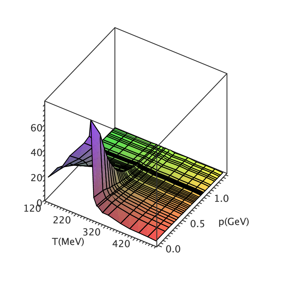
We plot the finite inverse of the propagators in Fig. 3. For IR momenta, they are again compatible with a massive denominator. Notice is linear in the infrared, while bends. In the UV the propagators have a logarithmica behavior, log.
The simplest ansatz for a massive propagator is,
| (9) |
The ersulting fit is shown in Fig. 4. Close to , clearly signals the transition, while is aparently flat. At , the two masses cross,
| 121 | 0.467 | 4.28(16) | 0.468(13) | 1.91 |
|---|---|---|---|---|
| 162 | 0.570 | 4.252(89) | 0.3695(73) | 1.66 |
| 194 | 0.330 | 5.84(50) | 0.381(22) | 0.72 |
| 243 | 0.330 | 8.07(67) | 0.374(21) | 0.27 |
| 260 | 0.271 | 8.73(86) | 0.371(25) | 0.03 |
| 265 | 0.332 | 7.34(45) | 0.301(14) | 1.03 |
| 275 | 0.635 | 3.294(65) | 0.4386(83) | 1.64 |
| 285 | 0.542 | 3.12(12) | 0.548(16) | 0.76 |
| 290 | 0.690 | 2.705(50) | 0.5095(85) | 1.40 |
| 305 | 0.606 | 2.737(80) | 0.5900(32) | 1.30 |
| 324 | 0.870 | 2.168(24) | 0.5656(63) | 1.36 |
| 366 | 0.716 | 2.242(55) | 0.708(13) | 1.80 |
| 397 | 0.896 | 2.058(34) | 0.795(11) | 1.03 |
| 428 | 1.112 | 1.927(24) | 0.8220(89) | 1.30 |
| 458 | 0.935 | 1.967(37) | 0.905(13) | 1.45 |
| 486 | 1.214 | 1.847(24) | 0.9285(97) | 1.55 |

Moreover we apply a better ansatz, adequate for IR momenta, we fit to a Yukawa with mass and dressing function
| (10) |
and look for the largest fitting range . While this fits quite well , the Yukawa ansatz does not fit . In Fig. 5 we show the fit of the mass and of the factor . While peaks at the transition, the mass is minimum but clearly finite.

5 Conclusion
We compute the gluon propagator in Landau gauge Lattice QCD at finite . The longitudinal component is peaked at . In the infrared, we fit with massive Yukawa ansatze, the fit to is more stable than the fit to . The fitted longitudinal gluon mass is compatible with confinement screening at . is also consistent with debye screening at , We observe is minimum at , but finite [7] as suggested by multiplicites of and production in heavy ion collisions.
References
- [1] J. M. Cornwall, Phys. Rev. D 26, 1453 (1982).
- [2] O. Oliveira and P. Bicudo, J. Phys. G 38, 045003 (2011) [arXiv:1002.4151 [hep-lat]].
- [3] N. Cardoso, M. Cardoso and P. Bicudo, Phys. Rev. D 88, 054504 (2013) [arXiv:1302.3633 [hep-lat]].
- [4] M. Doring, K. Huebner, O. Kaczmarek and F. Karsch, Phys. Rev. D 75, 054504 (2007) [hep-lat/0702009 [HEP-LAT]].
- [5] P. Bicudo, F. Giacosa and E. Seel, Phys. Rev. C 86, 034907 (2012) [arXiv:1202.1640 [hep-ph]].
- [6] U. M. Heller, F. Karsch and J. Rank, Phys. Rev. D 57, 1438 (1998) [hep-lat/9710033].
- [7] P. J. Silva, O. Oliveira, P. Bicudo and N. Cardoso, arXiv:1310.5629 [hep-lat].
- [8] N. Cardoso, P. J. Silva, P. Bicudo and O. Oliveira, Comput. Phys. Commun. 184, 124 (2013) [arXiv:1206.0675 [hep-lat]].
- [9] M. Schr’́oeck and H. Vogt, Comput. Phys. Commun. 184, 1907 (2013) [arXiv:1212.5221 [hep-lat]].
- [10] O. Oliveira and P. J. Silva, Phys. Rev. D 86, 114513 (2012) [arXiv:1207.3029 [hep-lat]].
- [11] D. Dudal, O. Oliveira and N. Vandersickel, Phys. Rev. D 81, 074505 (2010) [arXiv:1002.2374 [hep-lat]].
- [12] A. Maas, J. M. Pawlowski, L. von Smekal and D. Spielmann, Phys. Rev. D 85, 034037 (2012) [arXiv:1110.6340 [hep-lat]].
- [13] R. Aouane, V. G. Bornyakov, E. M. Ilgenfritz, V. K. Mitrjushkin, M. Muller-Preussker and A. Sternbeck, Phys. Rev. D 85, 034501 (2012) [arXiv:1108.1735 [hep-lat]].