Capacity Bounds for a Class of Diamond Networks

The diamond network was introduced in [1] as a simple multi-hop network with broadcast and multiple access channel (MAC) components. The two-relay diamond network models the scenario where a source communicates with a sink through two relay nodes that do not have information of their own to communicate. The underlying challenge may be described as follows. In order to fully utilize the MAC to the receiver, we would ideally like full cooperation between the relay nodes. On the other hand, in order to communicate the maximum amount of information and better use the diversity that is offered by the relays, we would like to send independent information to the relay nodes over the broadcast channel. The problem of finding the capacity of this network is unresolved. Lower and upper bounds on the capacity are given in [1]. We remark that the problem is solved over linear deterministic relay networks, and the capacity of Gaussian relay networks has been approximated within a constant number of bits [2].

In this paper, we study a class of diamond networks where the broadcast channel is modelled by two independent bit-pipes. This problem was initially studied in [3] where lower and upper bounds were derived on the capacity. The best known upper bound for the problem is the cut-set bound, which does not fully capture the tradeoff between cooperation and diversity. Recently, [4] studied the network with a Gaussian MAC and proved a new upper bound which constrains the mutual information between the MAC inputs to improve the cut-set bound. The bounding technique in [4] is motivated by [5] that treats the Gaussian multiple description problem. Unfortunately, neither result seems to apply to discrete memoryless channels.

This paper is organized as follows. We state the problem setup in Section II. In Section III, we prove a new upper bound on the achievable rates by generalizing the bounding technique of [4]. Our upper bound applies to the general class of discrete memoryless MACs, and strictly improves the cut-set bound. In Section IV, we improve the achievable rates of [3] by communicating a common piece of information from the source to both relays using superposition coding and Marton’s coding. Finally, we study our bounds for networks with a Gaussian MAC (Section V) and a binary adder MAC (Section VI). For both examples, we find conditions on the bit-pipe capacities such that the upper and lower bounds meet.

The idea behind our upper bound is motivated by [4, 5]. The proposed bound is applicable not only to Gaussian channels, but also to general discrete memoryless channels, and it strictly improves the cut-set bound as we show via two examples.

In the network of Fig. 1, the cut-set bound gives

However, the bound in (1) disregards the potential correlation between the inputs of the MAC. A tighter bound on $R$ is given in the following multi-letter form:

It is observed in [4] that $I(X_{1}^{n};X_{2}^{n})$ can be written in the following form for any random sequence $U^{n}$.

Therefore, we have

It may not be clear how to single-letterize the above bound. We proceed as follows. First, note that

Combining inequalities (5) and (6), we have

Define $U_{i}$ from $X_{1i},X_{2i},Y_{i}$ through the channels $p_{U_{i}|X_{1i}X_{2i}Y_{i}}(u_{i}|x_{1i},x_{2i},y_{i})$, $i=1,2,\ldots,n$. With this choice of $U_{i}$ we have the following chain of inequalities:

Step $(a)$ follows because we have the following two Markov chains:

We thus have the following upper bound.

We study the upper bound of Theorem 1 with a Gaussian MAC and a binary adder MAC in Sections V and VI respectively.

The achievable scheme that we present here is based on [3], but we further allow a common message at both relaying nodes. This is done by rate splitting, superposition coding and Marton’s coding and is summarized in the following theorem¹¹ 1 The method to derive this theorem was discussed in general terms by G. Kramer and S. Shamai after G. Kramer presented the paper [3] at ITW in 2007..

The output of the Gaussian MAC is given by

where $Z\sim\mathcal{N}(0,1)$, and the transmitters have average power constraints $P_{1},P_{2}$; i.e., $\frac{1}{n}\sum_{i=1}^{n}\mathbb{E}(X_{1,i}^{2})\leq P_{1}$ and $\frac{1}{n}\sum_{i=1}^{n}\mathbb{E}(X_{2,i}^{2})\leq P_{2}$.

We specialize Theorem 1 to obtain an upper bound on the achievable rate $R$. To simplify the bound, pick $U$ to be a noisy version of $Y$ in the form of $U=Y+Z_{N}$, where $Z_{N}$ is a Gaussian noise with zero mean and variance $N$ (to be optimized later). Inequalities (10)-(14) are upper bounded as follows using maximum entropy lemmas:

To obtain inequality $(a)$ above, write the RHS of (14) as

The negative terms are easy to calculate because of the Gaussian nature of the channel and the choice of $U$. The positive terms are bounded from above using the conditional version of the maximum entropy lemma [8]. It remains to solve a max-min problem (max over $\rho$ and min over $N$). So the rate $R$ is achievable only if there exists some $\rho>0$ for which for every $N>0$ inequalities (31)-(V) hold.

We choose $N$ to be (see [4, eqn. (21)])

Let us first motivate this choice. It is easy to see that inequality (V) is simply

evaluated for the joint Gaussian distribution $p(x_{1},x_{2})$ with covariance matrix

The choice (39) makes $U$ satisfy the Markov chain $X_{1}-U-X_{2}$ for the regime where

and thus minimizes the RHS of (V). Otherwise, $U=Y$ is chosen which results in a redundant bound. The upper bound is summarized in Corollary 1.

For a lower bound, we use Theorem 2 and choose $(U,X_{1},X_{2})$ to be jointly Gaussian with mean $0$ and covariance matrix $\mathbf{K}_{UX_{1}X_{2}}$. Fig. 2 shows the upper and lower bound as a function of $C$ for a symmetric network with $C_{1}=C_{2}=C$ and $P_{1}=P_{2}=1$. The dash-dotted curve in Fig. 2 shows the rates achievable using the scheme of Section IV with a joint Gaussian distribution. It is interesting to see that the obtained lower bound is not concave in $C$. This does not contradict Proposition 1 because Gaussian distributions are sub-optimal. The improved dashed curve shows rates that are achievable using a mixture of two Gaussian distributions.

For symmetric diamond networks where $C_{1}=C_{2}=C$ and $P_{1}=P_{2}=P$, we specify a regime of $C$ for which the lower and upper bounds meet and thus characterize the capacity. This is summarized in Theorem 3. See [6] for the proof.

For example, the upper and lower bounds match in Fig. 2 (where $P=1$) for $C\leq 0.3962$, $0.4807\leq C\leq 0.6942$, and $C\geq 1.1610$.

Consider the binary adder channel defined by $\mathcal{X}_{1}=\{0,1\}$, $\mathcal{X}_{2}=\{0,1\}$, $\mathcal{Y}=\{0,1,2\}$, and $Y=X_{1}+X_{2}$. The best known upper bound for this channel is the cut-set bound. We specialize Theorem 1 to derive a new upper bound on the achievable rate. For simplicity, we assume $C_{1}=C_{2}=C$.

Define $p(u|x_{1},x_{2},y)$ to be a symmetric channel as shown in Fig. 3, with parameter $\alpha$ to be optimized. From Theorem 1, the rate $R$ is achievable only if for some pmf $p(x_{1},x_{2})$ inequalities (10)-(14) hold for the aforementioned choice of $U$ and for every $\alpha$; i.e., we have to solve a max-min problem (max over $p(x_{1},x_{2})$, min over $\alpha$).

In the rest of this Section we manipulate the above bound to formulate a simplified upper bound. First, loosen the upper bound by looking at the min-max problem (rather than the max-min problem). Fix $\alpha$. For a fixed channel $p(u|x_{1},x_{2},y)$, the upper bound is concave in $p(x_{1},x_{2})$ (see Remark 2). The concavity, together with the symmetry of the problem and the auxiliary channel imply the following lemma.

Using Lemma 1, $p(x_{1},x_{2})$ may be assumed to be a doubly symmetric binary source with cross-over probability $p$. The bounds in (10)-(14) reduce to

The inequality in $(a)$ follows from (15) and the fact that $(X_{1}X_{2})-Y-U$ forms a Markov chain.

To obtain the best bound, we choose $U$ such that $X_{1}-U-X_{2}$ forms a Markov chain; i.e., the optimal $\alpha$ satisfies

where $p^{\star}$ is the $p$ which maximizes

Since we have $p^{\star}\leq\frac{1}{2}$, the choice (56) is valid and we therefore obtain Corollary 2.

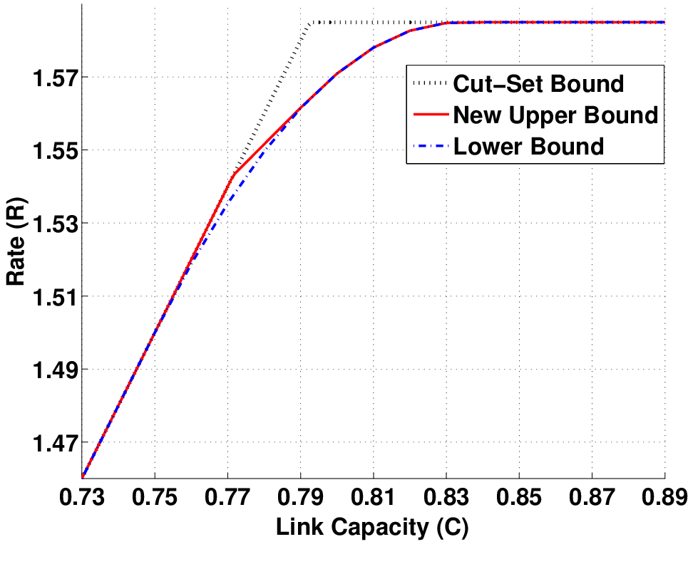
Fig. 4 plots this bound (Corollary 2) and compares it with the cut-set bound and the lower bound of Theorem 2 for different values of $C$. It turns out that the lower and upper bounds meet for $C\leq.75$ and $C\geq.7929$. See [6] for the proof.

The work of S. Saeedi Bidokhti was supported by the Swiss National Science Foundation fellowship no. 146617. The work of G. Kramer was supported by an Alexander von Humboldt Professorship endowed by the German Ministry of Education and Research.

References

• [1] B. E. Schein, Distributed coordination in network information theory. PhD Dissertation, MIT, 2001.
• [2] A. Avestimehr, S. Diggavi, and D. Tse, “Wireless network information flow: A deterministic approach,” IEEE Trans. Inf. Theory, vol. 57, no. 4, pp. 1872 –1905, april 2011.
• [3] D. Traskov and G. Kramer, “Reliable communication in networks with multi-access interference,” in Proc. Inf. Theory Workshop, 2007.
• [4] W. Kang and N. Liu, “The gaussian multiple access diamond channel,” in Proc. Int. Symp. Inf. Theory, 2011.
• [5] L. Ozarow, “On a source-coding problem with two channels and three receivers,” Bell System Technical Journal, vol. 59, no. 10, pp. 1909–1921, 1980.
• [6] S. Saeedi Bidokhti and G. Kramer, “Capacity bounds for a class of diamond networks,” Jan. 2014. [Online]. Available: https://mediatum.ub.tum.de/doc/1189765/1189765.pdf
• [7] A. El Gamal and Y. H. Kim, Network Information Theory. Cambridge University Press, 2011.
• [8] J. Thomas, “Feedback can at most double gaussian multiple access channel capacity (corresp.),” IEEE Trans. Inf. Theory, vol. 33, no. 5, pp. 711–716, 1987.