Sequential Joint Spectrum Sensing and Channel Estimation for Dynamic Spectrum Access

As a fundamental requirement in cognitive radio systems, the SUs should not cause degradation in the quality of service (QoS) to the PUs. In other words, the interference from the SUs to the PUs must be kept below some maximum tolerable levels. Under such interference constraints, a natural objective is to maximize the SU throughput, i.e., the average bit-rate of SU Tx. Hence, assuming Gaussian noise in channels between the PUs and also between the SUs we aim to solve the following optimization problem

where $P(h_{11},h_{21})$ is the transmit power of SU Tx, constrained by the maximum power $P_{\text{max}}$, and is a function of the channel gains $h_{11},h_{21},$ between SU Tx and the PUs; $\beta$ and $N_{0}$ are the channel gain and the variance of the Gaussian noise, respectively, between SU Tx and SU Rx; $Q_{1}$ and $Q_{2}$ are the transmit powers for PUs; and $I_{1}$ and $I_{2}$ are the maximum tolerable interference powers at PUs, which are determined by the PU outage constraints. The null hypothesis $\mathsf{H}_{0}$ and the alternative hypothesis $\mathsf{H}_{1}$ correspond to the absence and presence of PU communication, respectively. More specifically, $Q_{1}=Q_{2}=0$ under $\mathsf{H}_{0}$, whereas $\max\{Q_{1},Q_{2}\}\not=0$ under $\mathsf{H}_{1}$.

In (1), we in fact maximize the average capacity of a Gaussian channel, where the interference constraint $I_{1}$ is determined according to the outage constraint on another Gaussian channel $g_{1}$

where $\eta_{1}$ is the variance of the Gaussian noise; and $R_{2}$ is the bit-rate of PU $2$. The outage constraint in (2) yields the interference constraint in (1), given $Q_{2},R_{2},\eta_{1},\mathsf{P}_{\text{out}}$. The maximum interference value $I_{2}$ is written similarly. We assume $I_{1}$ and $I_{2}$ are available to SUs. In a careful design, there should be some safety margin between the probability on the left hand-side of (2) and $\mathsf{P}_{\text{out}}$ while determining $I_{i}$. This is because SUs may unintentionally exceed $I_{i}$ due to lack of information on the true hypothesis and the actual channel coefficients.

The conventional spectrum access methods for cognitive radio, namely the opportunistic access and underlay methods, provide simplistic solutions to (1). In particular, the opportunistic access method focuses only on the binary hypothesis test, i.e., spectrum sensing, and conforms to the interference constraints by simply turning off SU Tx, i.e., $P=0$, when $\mathsf{H}_{1}$ is declared. When $\mathsf{H}_{0}$ is declared, SU Tx transmits at the maximum power, i.e., $P=P_{\text{max}}$. On the other hand, the underlay method does not perform spectrum sensing and solves only the constrained optimization problem under $\mathsf{H}_{1}$. As a result, the constant power $P=\min\left\{P_{\text{max}},\frac{I_{1}}{|h_{11}|^{2}},\frac{I_{2}}{|h_{21}|^{2}}\right\}$ is transmitted under both $\mathsf{H}_{0}$ and $\mathsf{H}_{1}$. It is seen that deep fades in the cross links $\{h_{ik}\}$ are beneficial for the SU throughput.

In practice, the channels $g_{1},g_{2}$ between the PUs, and the cross links $\{h_{ik}\}$ are not known a priori. Hence, the PUs perform a preamble communication with duration $T_{p}$ at the beginning of each data transmission frame to estimate $g_{1}$ and $g_{2}$. Specifically, for transmission frame $m$, as shown in Fig. 2, PU $i$ estimates $g_{i}$ during $t\in\big(T(m-1),T(m-1)+T_{p}\big]$ using pilot symbols, and then data transmission takes place during $t\in\big(T(m-1)+T_{p},Tm\big]$, where $T$ is the frame duration. Assuming the SUs are synchronized with the PU frame timing and observe pilot signals, each SU can estimate its cross links during each preamble period.

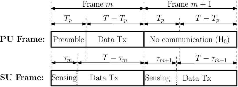
As opposed to the naive solutions of the conventional spectrum access methods, an efficient solution to (1) should involve both spectrum sensing and channel estimation, hence it is a combination of the opportunistic access and underlay methods. For example, at a fixed time $\tau\in(0,T_{p}]$, we can employ the optimum detector, i.e., the likelihood ratio test (LRT) for spectrum sensing, and the optimum estimator, i.e., the minimum mean square error (MMSE) estimator for channel estimation. Once we obtain the spectrum sensing result ($\mathsf{H}_{0}$ or $\mathsf{H}_{1}$) and the channel estimates $\{\hat{h}_{ik}\}$, we can use them to solve (1) as follows: SU Tx transmits with $P=P_{\text{max}}$ when $\mathsf{H}_{0}$ is declared, as in opportunistic access, and with $P=\min\left\{P_{\text{max}},\frac{I_{1}}{|\hat{h}_{11}|^{2}},\frac{I_{2}}{|\hat{h}_{21}|^{2}}\right\}$ when $\mathsf{H}_{1}$ is declared, as in underlay.

As a more sophisticated example, instead of performing fixed-sample-size detection and estimation (at a fixed time $\tau$) we can determine the sample number based on the observed samples, resulting in a sequential method with a random sensing time $\tau$. In particular, we can use the sequential probability ratio test (SPRT) [24], which is the optimum sequential detector for i.i.d. observations in terms of minimizing the average detection delay, for spectrum sensing, and then use the MMSE estimator at the random sensing time $\tau$ to estimate the unknown channel gains $\{h_{ik}\}$.

However, the above approaches based on separate detection and estimation in general may not yield the optimal solution. In the following section, we propose a new and powerful solution based on sequential joint detection and estimation.

In our system model, in each frame $m$ during the preamble period $t\in\big(T(m-1),T(m-1)+T_{p}\big]$, the signal received by the SU from PU $i$ is given by

where $w_{i}[t]\sim\mathcal{N}_{c}(0,N_{0}^{i})$ is the complex additive white Gaussian noise; $h_{i}\sim\mathcal{N}_{c}(\mu_{i},\sigma_{i}^{2})$ is the proper complex channel coefficient between PU $i$ and the SU; and $p_{i}[t]$ is the complex random pilot signal used in the preamble. The processes $\{p_{i}[t]\}$ and $\{w_{i}[t]\}$ are independent and they are independent of the random variable $h_{i}$. We assume the SU observes $p_{i}[t]$ at time $t$, e.g., the SU knows the seed of the random number generator that generates $p_{i}[t]$, for $i=1,2$.

In (3), we would like to decide between $\mathsf{H}_{0}$ and $\mathsf{H}_{1}$ as soon as possible, and also estimate $h_{i}$ if we decide for $\mathsf{H}_{1}$. In other words, our objective is to have a reliable estimate of the channel coefficient $h_{i}$ every time we detect the presence of PU communication. Deciding as soon as possible is important because an early sensing time, i.e., small $\tau$, enables the SU to transmit data for a longer period of time, i.e., large $T-\tau$, increasing the SU throughput. On the other hand, the SU transmit power, which is a function of sensing decision and estimates of $\{h_{1},h_{2}\}$, should obey the PU maximum interference constraints. Small $\tau$ may increase the misdetection probability and decrease the estimation accuracy, leading to the violation of such constraints and PU outage. Hence, there is a tradeoff in selecting the $\tau$ value. Conventionally $\tau$ is selected offline, resulting in a fixed-sample-size test. Whereas in a sequential test $\tau$ is determined online, i.e., it depends on the observations, and thus it is random. Although sequential tests are more sophisticated than fixed-sample-size tests, they are much more powerful in minimizing the average sensing time, $\mathsf{E}[\tau]$, hence suit better the cognitive radio application.

In the separate detection and estimation approach, the unknown channel gain $h_{i}$ is treated as a nuisance parameter while performing detection. However, channel estimation is an integral part of the problem of interest. Hence, formulating the problem as a joint detection and estimation problem is a more natural way to obtain better overall performance, i.e., SU throughput. Indeed it was shown in [13] that the combined optimum detector and optimum estimator do not produce the optimum overall detection and estimation performance.

Since the results in [13] are obtained for real signals, for analytical convenience in our problem we will treat a complex observation (channel) as two real observations (channels). Specifically, we compute $y_{i}^{1}[t]\triangleq\Re(p_{i}[t]^{*}y_{i}[t])$ and $y_{i}^{2}[t]\triangleq\Im(p_{i}[t]^{*}y_{i}[t])$, hence instead of (3) we use the following signal model

where $h_{i}^{1}\triangleq\Re(h_{i})$, $h_{i}^{2}\triangleq\Im(h_{i})$, $w_{i}^{1}[t]\triangleq\Re(p_{i}[t]^{*}w_{i}[t])$, and $w_{i}^{2}[t]\triangleq\Im(p_{i}[t]^{*}w_{i}[t])$. Note in (4) that $h_{i}^{n}\sim\mathcal{N}\left(\frac{\mu_{i}}{2},\frac{\sigma_{i}^{2}}{2}\right),n=1,2~$; and given $p_{i}[t]$, the noise $w_{i}^{n}[t]\sim\mathcal{N}\left(0,|p_{i}[t]|^{2}\frac{N_{0}^{i}}{2}\right),n=1,2$, and $\{w_{i}^{n}[t]\}$ are independent across channels (for different $i$) and time. Similar to (3), we want to sequentially decide between $\mathsf{H}_{0}$ and $\mathsf{H}_{1}$, and also estimate $h_{i}^{n}$ when we decide on $\mathsf{H}_{1}$. To present the sequential joint detection and estimation (SJDE) problem and the optimum solution to it we first focus on a single channel case, i.e., the signal model in (4) for specific $i,n$ values. In particular, the SU, using its observations $\left\{(y_{i}^{n}[t],p_{i}[t])\right\}_{t}$ through the real channel $n$ linked to PU $i$, wants to jointly detect the PU communication and estimate the channel coefficient $h_{i}^{n}$ when it decides on its presence.

In sequential methods, in general, the average sample number, which corresponds to the average sensing time in our context, is minimized subject to a set of constraints, e.g., false alarm and misdetection constraints for detection, and mean squared error constraint for estimation. In the proposed joint framework we use the following combined cost function

where $d_{\tau}$ is the decision function; $x\triangleq h_{i}^{n}$ is the unknown parameter; $\hat{x}_{\tau}$ is the estimate of $x$; $c_{0},c_{1},c_{e}$ are nonnegative constants selected by the designer; $\mathsf{P}_{0}$ and $\mathsf{E}_{0}$ denote the probability measure and expectation under hypothesis $\mathsf{H}_{0}$; $\bar{\mathsf{P}}_{1}$ and $\bar{\mathsf{E}}_{1}$ denote the probability measure and expectation under $\mathsf{H}_{1}$; $\mathsf{P}_{1}$ and $\mathsf{E}_{1}$ denote the probability measure and expectation under $\mathsf{H}_{1}$ with $x$ being marginalized; $\mathcal{F}_{t}=\sigma\left\{p_{i}[1],\ldots,p_{i}[t]\right\}$ is the $\sigma$-algebra, that is, the accumulated history pertinent to the observed process $\left\{p_{i}[t]\right\}$; and $\mathbbm{1}_{\{A\}}$ is the indicator of the event $A$, taking the value $1$ if $A$ occurs and $0$ otherwise. Then, our constrained optimization problem is given by

where $\alpha>0$ is a given constant, denoting the target accuracy level.

Our formulation in (5) and (6) is conditioned on the auxiliary statistic $\mathcal{F}_{t}$ because using such extra information we can assess the accuracy of the detector and estimator more precisely than the unconditional formulation. More specifically, since $\mathsf{P}_{0}\left(d_{\tau}=1\right)=\mathsf{E}_{0}\left[\mathbbm{1}_{\{d_{\tau}=1\}}\right]=\mathsf{E}\left[\mathsf{E}_{0}\left[\mathbbm{1}_{\{d_{\tau}=1\}}|\mathcal{F}_{\tau}\right]\right]=\mathsf{E}\left[\mathsf{P}_{0}\left(d_{\tau}=1|\mathcal{F}_{\tau}\right)\right]$, there is no need to use the expectation, e.g., $\mathsf{P}_{0}\left(d_{\tau}=1\right)$, of an accuracy assessment term when the term itself, e.g., $\mathsf{P}_{0}\left(d_{\tau}=1|\mathcal{F}_{\tau}\right)$, is available. Moreover, with the conditional formulation used in (5) we do not need to specify the distribution of the pilot signal $p_{i}[t]$. Note that the constraint $\mathcal{C}\left(\tau,d_{\tau},\hat{x}_{\tau}\right)\leq\alpha$ in (6) is required to hold for each realization of the process $\left\{p_{i}[t]\right\}$, hence is stricter than its unconditional counterpart, which is required to hold only on average with respect to $\left\{p_{i}[t]\right\}$.

In (5), the first two terms, which are related to the detection problem, correspond to the false alarm and misdetection probabilities ($\mathsf{P}_{f}$ and $\mathsf{P}_{m}$), respectively. On the other hand, the last term, which is related to the estimation problem, depends on both the decision and estimation strategies. Without this term, i.e., for $c_{e}=0$, the combined cost depends only on the decision function $d_{\tau}$, implying that the joint problem reduces into a pure detection problem.

Similar to $\mathcal{F}_{t}$ let $\mathcal{G}_{t}=\sigma\left\{(y_{i}^{n}[1],p_{i}[1]),\ldots,(y_{i}^{n}[t],p_{i}[t])\right\}$ denote the $\sigma$-algebra generated by the processes $\{y_{i}^{n}[t]\}$ and $\left\{p_{i}[t]\right\}$, i.e., the complete observation history. Then, we have the corresponding filtrations $\{\mathcal{F}_{t}\}_{t\geq 0}$ and $\{\mathcal{G}_{t}\}_{t\geq 0}$. In general, the solution we seek should use all available information, that is, we are looking for a triplet $(\tau,d_{\tau},\hat{x}_{\tau})$ where $\tau$ is $\{\mathcal{G}_{t}\}$-adapted, $d_{\tau}$ and $\hat{x}_{\tau}$ are $\mathcal{G}_{\tau}$-measurable. It is known in the pure estimation problem that with a $\{\mathcal{G}_{t}\}$-adapted stopping time $\tau$, in most cases, finding an optimum sequential estimator $(\tau,\hat{x}_{\tau})$ is not tractable [25]. Instead, [26] considered using an $\{\mathcal{F}_{t}\}$-adapted stopping time, which was later shown to have a simple optimal solution for continuous-time and discrete-time observations in [27] and [23], respectively. Similarly, in the pure detection problem with a $\{\mathcal{G}_{t}\}$-adapted $\tau$ we have a two-dimensional optimal stopping problem, which is not tractable. Consequently, following the approach used for the pure estimation problem in [26, 27, 23] we consider $\{\mathcal{F}_{t}\}$-adapted stopping times for our joint problem. On the other hand, we are still interested in $\mathcal{G}_{\tau}$-measurable decision rule $d_{\tau}$ and estimator $\hat{x}_{\tau}$, which use all available information acquired up to stopping time $\tau$. As a result, the problem in (6) takes the following form

The following theorem gives the optimum solution to the above problem.

Comparing the optimum triplet in Theorem 1 with the combined SPRT & MMSE method, we see that there are fundamental differences in the stopping rule and decision function. In SPRT [28], the stopping time and detection decision are determined together through a common procedure. More specifically, two thresholds are used to jointly terminate the scheme and make a decision. When the scheme terminates, the decision is already clear as it is determined by the threshold that causes termination. As a result, the performance metrics $\mathsf{P}_{f}$, $\mathsf{P}_{m}$, $\mathsf{E}[\tau]$, and also MSE$=\mathsf{E}[(\hat{x}_{\tau}-x)^{2}]$ are closely interrelated since they are all controlled by the two thresholds, which are the only system parameters. On the other hand, in SJDE the stopping time and decision are computed using two separate procedures. First the stopping time is found by performing a single-threshold-test, and then the decision is made via a modified LRT. In particular, $\mathsf{E}[\tau]$ and $\mathsf{E}[(\hat{x}_{\tau}-x)^{2}]$ are controlled by only the stopping threshold $\gamma$, whereas $\mathsf{P}_{f}$ and $\mathsf{P}_{m}$ are controlled by $\gamma$, $c_{0}$, $c_{1}$, and $c_{e}$. That is to say, $\mathsf{E}[\tau]$ and $\mathsf{E}[(\hat{x}_{\tau}-x)^{2}]$ can be controlled independently from $\mathsf{P}_{f}$ and $\mathsf{P}_{m}$ through $\gamma$, and similarly $\mathsf{P}_{f}$ and $\mathsf{P}_{m}$ can be controlled independently from $\mathsf{E}[\tau]$ and $\mathsf{E}[(\hat{x}_{\tau}-x)^{2}]$ through $c_{0}$, $c_{1}$, and $c_{e}$. The latter set of parameters enables a trade-off between $\mathsf{P}_{f}$ and $\mathsf{P}_{m}$ without affecting $\mathsf{E}[\tau]$ and $\mathsf{E}[(\hat{x}_{\tau}-h_{i}^{n})^{2}]$. For instance, we can trade false alarm probability $\mathsf{P}_{f}$ for misdetection probability $\mathsf{P}_{m}$, which is crucial for complying with the outage constraints of PUs, by decreasing the ratio of $c_{0}$ to $c_{1}$ or $c_{e}$ without sacrificing early stopping or estimation quality. We obviously have a higher degree of freedom in SJDE than SPRT due to the number of parameters that control the system performance, which endows us with the ability to strike a right balance between our objectives of early stopping, and accurate detection and estimation.

In Fig. 3, we numerically show the superior performance of SJDE over the combined SPRT & MMSE (SPRT&E) in terms of the combined detection and estimation cost in (5). We also compare SJDE with the sequential LRT & MMSE (SLRT&E) that is equipped with the stopping rule of SJDE to demonstrate the advantage of incorporating the estimate into the decision function. SLRT&E uses the unmodified (original) LRT to detect, hence can be seen as a separate-formulation-method. It outperforms SPRT&E since it enjoys the flexibility of SJDE to strike a desired balance for the specific problem of interest by employing two separate procedures, namely the stopping rule of SJDE and LRT, to terminate the scheme and make a decision respectively. In our problem of interest, it is crucial that SUs do not violate the maximum interference constraint, which in turn ensures an admissible PU outage probability. In case of misdetection the SU transmits with maximum power, which may cause the violation of outage constraint. Even when the SU correctly detects PU communication, poor channel estimate may still cause the SU to transmit with a non-admissible power. On the other hand, the false alarm, which corresponds to deciding on $\mathsf{H}_{1}$ under $\mathsf{H}_{0}$, is not related to the outage constraint, but only degrades the SU throughput. Therefore, in the combined cost expression in (5) the second and third terms are more important than the first term. Accordingly, in Fig. 3 we use $c_{0}=c_{1}=0.2$ and $c_{e}=0.6$. Since the second part of the third term in (5) already penalizes misdetection, we do not differentiate between the coefficients, $c_{0}$ and $c_{1}$, of the detection error probabilities. In Fig. 3, referring to (4) we use $\mu_{i}=0$, i.e., Rayleigh fading channel $h_{i}^{n}$, and $\sigma_{i}^{2}=N_{0}^{i}=\mathsf{E}[|p_{i}[t]|^{2}]=1$.

Here, following the optimum SJDE scheme in Theorem 1 for the single channel case we are interested in finding the optimum SJDE scheme for the SU observing the signals $\left\{y_{i}^{n}[t]\right\}$ and $\left\{p_{i}[t]\right\}$ through the channels $\left\{h_{i}^{n}\right\},~i=1,2,~n=1,2$ from PU $1$ and PU $2$. We first need to modify the cost function in (5) by adding the new MSE terms, i.e.,

The following theorem, whose proof is provided in the Appendix, gives the optimum SJDE scheme in this case.

For systems with multiple SU pairs, in the next section we propose a distributed and cooperative spectrum access method which selects the SU with the maximum achievable throughput, and controls its transmit power.

We now consider the multi-SU case for SJDE, and propose a dynamic spectrum access method (DSA-SJDE). From (13), we have the following cost function,

Note that all $K$ SUs observe the same pilot signals $\left\{p_{1}[t]\right\}$ and $\left\{p_{2}[t]\right\}$. Hence, from (14) it is seen that they have the same stopping time, which in this case serves as a global stopping time. Each channel coefficient $h_{ik}^{n}$ is again estimated using (17) for all $k,i,n$ because they are independent. Since the observations $\left\{y_{ik}^{n}[t]\right\}_{k}$, across SUs, are independent given $\left\{p_{i}[t]\right\}$, the global LLR is written as $L_{t}=\sum_{k=1}^{K}L_{t}^{k}$, and as in (2) we sum the channel estimates to write the threshold. Then, substituting the global LLR and the global threshold in (2) we obtain the decision function for the multi-SU case.

It looks like the SJDE scheme for the multi-SU case simply follows from (14)–(17) in the single-SU case. However, in the multi-SU case the stopping time, detector, and estimator are computed at the FC, which requires some local information. Note that the FC can reasonably observe the pilot signals $\left\{p_{1}[t]\right\}$ and $\left\{p_{2}[t]\right\}$ in the same way SUs do. Then, the FC needs to know the local random variables $\left\{V_{\tau}^{ikn}\right\}_{i,k,n}$ at the stopping time $\tau$. In a straightforward way SUs can quantize and send $\left\{V_{\tau}^{ikn}\right\}_{i,k,n}$ at time $\tau$. However, this method has several disadvantages in practice. Firstly, it needs high bandwidth at time $\tau$ on each reporting channel between SUs and the FC. Moreover, the reporting channels are utilized inefficiently. They remain idle until time $\tau$, and at time $\tau$ each SU sends a number of bits, which may cause congestion at the FC. To overcome these practical issues SUs can sequentially report $\left\{V_{\tau}^{ikn}\right\}_{i,k,n}$. For sequential reporting level-triggered sampling, a non-uniform sampling technique, was shown to be much superior to the traditional uniform sampling in terms of bandwidth and energy requirements for detection and estimation purposes in [22] and [23], respectively. Therefore, we propose that SUs sequentially report $\left\{V_{\tau}^{ikn}\right\}_{i,k,n}$ using level-triggered sampling.

Each SU $k$, via the same level-triggered sampling procedure, informs the FC whenever considerable change occurs in its four local processes $\left\{V_{t}^{ikn}\right\},~i=1,2,~n=1,2$. In other words, $4K$ identical samplers run in parallel for $4K$ different processes. Hence, we will describe the procedure for a single process $\left\{V_{t}^{ikn}\right\}_{t}$. The level-triggered sampling is a simple form of event-triggered sampling, in which sampling (communication) times $\{t_{m}\},~m\in\mathbb{N},$ are not deterministic, but rather dynamically determined by the random process $\left\{V_{t}^{ikn}\right\}_{t}$, i.e.,

The threshold parameter $\Delta$ is a constant known by both SUs and the FC. At each sampling time $t_{m}$, SU $k$ transmits $r$ bits, $b_{m,1}b_{m,2}\ldots b_{m,r}$, to the FC. The first bit, $b_{m,1}$, indicates the threshold crossed (either $\Delta$ or $-\Delta$) by the incremental process $v_{m}\triangleq V_{t_{m}}^{ikn}-V_{t_{m-1}}^{ikn}$, i.e.,

The remaining $r-1$ bits are used to quantize the over(under)shoot $q_{m}\triangleq|v_{m}|-\Delta$ into $\tilde{q}_{m}$. At each sampling time $t_{m}$, the overshoot value $q_{m}$ cannot exceed the magnitude of the last sample $|y_{ik}^{n}[t_{m}]|$ in the incremental process $v_{m}=\sum_{t=t_{m-1}+1}^{t_{m}}y_{ik}^{n}[t]$. The quantization interval $[0,\phi]$ is uniformly divided into $2^{r-1}$ subintervals with the step size $\frac{\phi}{2^{r-1}}$. The mid value of each subinterval is used as the corresponding quantization level, i.e., a mid-riser quantizer is used. When $q_{m}>\phi$, the uppermost quantization level is used. The parameter $\phi$ is determined so that $\mathsf{P}(q_{m}>\phi)$ is sufficiently small. From [22, Section IV-B] we can set the threshold $\Delta$ using

for the FC to receive messages with an average rate of $M$ messages per unit time under $\mathsf{H}_{i},~i=0,1$. In Fig. 4, the level-triggered sampling procedure is demonstrated on a sample path of $V_{t}^{ikn}$.

The FC, upon receiving the bits $b_{m,1}b_{m,2}\ldots b_{m,r}$ from SU $k$ at time $t_{m}$, recovers the quantized value of $v_{m}$ by computing

Then, it sequentially sums up $\{\tilde{v}_{m}\}$, at the sampling (communication) times $\{t_{m}\}$ to obtain an approximation $\tilde{V}_{t}^{ikn}$ to the sufficient statistic $V_{t}^{ikn}$, i.e.,

where $M_{t}$ is the number of messages that the FC receives from SU $k$ about the process $\{V_{t}^{ikn}\}$ up to time $t$. During the times the FC receives no message, i.e., $t\not\in\{t_{m}\}$, $\tilde{V}_{t}^{ikn}$ is kept constant.

At the stopping time $\tau$, given by (14), the FC estimates each channel coefficient $h_{ik}^{n}$ using

and decides according to the following rule

where $\tilde{L}_{\tau}=\sum_{k=1}^{K}\sum_{i=1}^{2}\sum_{n=1}^{2}\tilde{L}_{\tau}^{ikn}$, and $\tilde{L}_{\tau}^{ikn}$ is computed from (12) by substituting $\tilde{V}_{t}^{ikn}$ for $V_{t}^{ikn}$. After making a decision, the FC grants the transmission privilege to the SU Tx with the highest achievable throughput. When the decision is in favor of $\mathsf{H}_{0}$, i.e., $\tilde{d}_{\tau}=0$, one of them is selected randomly (or in some specific order) since in this case any SU Tx can transmit with its maximum power $P_{\text{max}}$. On the other hand, when $\tilde{d}_{\tau}=1$, the FC selects SU Tx $k^{*}$ where

$k_{t}$ is the SU Tx index, and $|\tilde{h}_{ik}[\tau]|^{2}=\sum_{n=1}^{2}\left(\tilde{h}_{ik}^{n}[\tau]\right)^{2},~i=1,2$. The pseudocodes for the procedures at SU $k$ and the FC in the proposed SJDE-based dynamic spectrum access method (DSA-SJDE) are given in Algorithms 1 and 2, respectively. In Algorithm 1, an SU Rx never executes lines 17-23 since the FC reports $d_{\tau}$ to SU Tx $k^{*}$ (cf. line 20 in Algorithm 2).

References

- [1] Q. Zhao and B. M. Sadler, “A survey of dynamic spectrum access: Signal processing, networking, and regulatory policy,” IEEE Signal Processing Mag., vol.24, no. 3, pp. 79–89, May 2007.
- [2] X. Kang, Y. C. Liang, A. Nallanathan, H. K. Garg, and R. Zhang, “Optimal power allocation for fading channels in cognitive radio networks: ergodic capacity and outage capacity,” IEEE Trans. Wireless Commun., vol. 8, no.2, pp. 940–950, Feb. 2009.
- [3] L. Musavian and S. Aissa, “Capacity and power allocation for spectrum sharing communications in fading channels,” IEEE Trans. Wireless Commun., vol. 8, no.1, pp. 148–156, 2009.
- [4] X. Kang, R. Zhang, Y. C. Liang, and H. K. Garg, “Optimal power allocation strategies for fading cognitive radio channels with primary user outage constraint,” IEEE J. Sel. Areas Commun., vol. 29, no. 2, pp. 374–383, 2011.
- [5] Y. C. Liang, Y. Zeng, E. C. Y. Peh, and A. T. Hoang, “Sensing-throughput tradeoff for cognitive radio networks,” IEEE Trans. Wireless Commun., vol.7, no. 4, pp. 1326–1337, Apr. 2008.
- [6] Y. Chen, Q. Zhao, and A. Swami, “Joint design and separation principle for opportunistic spectrum access in the presence of sensing errors,” IEEE Trans. Inf. Theory, vol. 54, no. 5, pp. 2053–2071, May 2008.
- [7] R. Fan, H. Jiang, Q. Guo, and Z. Zhang, “Joint optimal cooperative sensing and resource allocation in multichannel cognitive radio networks,” IEEE Tran. Veh. Technol., vol. 60, no. 2, pp. 722–729, Feb. 2011.
- [8] N. Devroye, P. Mitran, and V. Tarokh, “Achievable rates in cognitive radio channels,” IEEE Trans. Inf. Theory, vol. 52, no. 5, pp. 1813–1827, May 2006.
- [9] X. Kang, Y. C. Liang, H. K. Garg, and L. Zhang, “Sensing-based spectrum sharing in cognitive radio networks”, IEEE Trans. Veh. Technol., vol. 58, no. 8, pp. 4649–4654, Oct. 2009.
- [10] R. Zhang, “On peak versus average interference power constraints for protecting primary users in cognitive radio networks”, IEEE Trans. Wireless Commun., vol. 8, no. 4, pp. 2112–2120, Apr. 2009.
- [11] Z. Chen, X. Wang, and X. Zhang, “Continuous power allocation strategies for sensing-based multiband spectrum sharing,” IEEE J. Sel. Areas Commun., to be published.
- [12] G. V. Moustakides, G. H. Jajamovich, A. Tajer, and X. Wang, “Joint detection and estimation: optimum tests and applications,” IEEE Trans. Inf. Theory, vol. 58, no. 7, pp. 4215–4229, July 2012.
- [13] Y. Yilmaz, G. V. Moustakides, and X. Wang, “Sequential joint detection and estimation,” SIAM Theory Probab. Appl., to be published, http://arxiv.org/abs/1302.6058.
- [14] D. Middleton and R. Esposito, “Simultaneous optimum detection and estimation of signals in noise,” IEEE Trans. Inf. Theory, vol. IT-14, no. 3, pp. 434–444, May 1968.
- [15] A. Fredriksen, D. Middleton, and D. Vandelinde, “Simultaneous signal detection and estimation under multiple hypotheses,” IEEE Trans. Inf. Theory, vol. IT-18, no. 5, pp. 607–614, Sep. 1972.
- [16] G. Yue, X. Zhou, and X. Wang, “Performance comparisons of channel estimation techniques in multipath fading CDMA,” IEEE Trans. Wireless Commun., vol.3, no. 3, pp. 716–724, May 2004.
- [17] Y. Li, “Pilot-symbol-aided channel estimation for OFDM in wireless systems,” IEEE Trans. Veh. Technol., vol. 49, no. 4, pp. 1207–1215, July 2000.
- [18] H. Tang, “Some physical layer issues of wide-band cognitive radio systems,” in Proc. IEEE Int. Symposium on New Frontiers in Dynamic Spectrum Access Networks, Baltimore, Maryland, USA, pp. 151–159, Nov. 2005.
- [19] A. Sahai, R. Tandra, S. M. Mishra, and N. Hoven, “Fundamental design tradeoffs in cognitive radio systems,” in Proc. of Int. Workshop on Technology and Policy for Accessing Spectrum, Aug. 2006.
- [20] S. M. Mishra, S. t. Brink, R. Mahadevappa, and R. W. Brodersen, “Cognitive technology for ultra-wideband/WiMax coexistence,” in Proc. IEEE Int. Symposium on New Frontiers in Dynamic Spectrum Access Networks, Dublin, Ireland, pp. 179–186, Apr. 2007.
- [21] G. Fellouris and G.V. Moustakides, “Decentralized sequential hypothesis testing using asynchronous communication,” IEEE Trans. Inf. Theory, vol. 57, no. 1, pp. 534–548, Jan. 2011.
- [22] Y. Yilmaz, G.V. Moustakides, and X. Wang, “Cooperative sequential spectrum sensing based on level-triggered sampling,” IEEE Trans. Signal Process., vol. 60, no. 9, pp. 4509–4524, Sep. 2012.
- [23] Y. Yilmaz, and X. Wang, “Sequential Decentralized Parameter Estimation under Randomly Observed Fisher Information,” IEEE Trans. Inf. Theory, to be published, http://arxiv.org/abs/1211.3720.
- [24] A. Wald and J. Wolfowitz, “Optimum character of the sequential probability ratio test,” Ann. Math. Stat., vol. 19, pp. 326-329, 1948.
- [25] B.K. Ghosh, “On the attainment of the Cramer-Rao bound in the sequential case,” Sequential Analysis, vol. 6, no. 3, pp. 267–288, 1987.
- [26] P. Grambsch, “Sequential sampling based on the observed Fisher information to guarantee the accuracy of the maximum likelihood estimator,” Ann. Statist., vol. 11, no. 1, pp. 68–77, 1983.
- [27] G. Fellouris, “Asymptotically optimal parameter estimation under communication constraints,” Ann. Statist., vol. 40, no. 4, pp. 2239–2265, Aug. 2012
- [28] A. Wald, Sequential Analysis, Wiley, New York, NY, 1947.
- [29] H.V. Poor, An Introduction to Signal Detection and Estimation, Springer, New York, NY, 1994.