Nonergodic Subdiffusion from Brownian Motion in an Inhomogeneous Medium

Disordered systems exhibiting subdiffusion have been studied intensively for decades [1, 2, 3, 4, 5]. In these systems the ensemble averaged mean squared displacement (EMSD) grows for large times as

whereas normal diffusion has $\beta=1$. A broad class of systems show weak ergodicity breaking, that is, the EMSD and the time averaged mean squared displacement (TMSD) differ. The prototypical framework for describing non-ergodic subdiffusion is the heavy-tailed continuous-time random walk (CTRW) [6, 7, 8], in which a particle takes steps at random time intervals that are independently distributed with density

$\psi({\tau})$ has infinite mean, which leads to a subdiffusive EMSD $\beta=\alpha$. Furthermore, the CTRW shows weak ergodicity breaking because the particle experiences trapping times on the order of the observation time $T$ no matter how large $T$ is. The CTRW was introduced to describe charge carriers in amorphous solids [8], and has found wide application since. Recently, there has been a surge of work on the CTRW [9, 10, 11, 12], triggered by single particle tracking experiments in biological systems [13, 14, 15, 16, 17] that display signatures of non-ergodicity.

A different approach to subdiffusion is to assume a deterministic diffusivity (i.e. diffusion coefficient) that is inhomogeneous in time [18, 19], or space [20, 21, 22, 23, 24]. But in fact, the anomalous diffusion in these works is also non-ergodic. Formulating models of inhomogeneous diffusivity is timely and important, given that recently measured spatial maps in the cell membrane often show patches of strongly varying diffusivity [25, 26, 27, 28, 29, 30]. The presence of randomness in these experimental maps inspired us to consider disordered media. Thus, in this manuscript, we introduce a class of models of ordinary diffusion with a diffusivity that varies randomly but is constant on patches of random sizes. We call these models random patch models or just patch models. These models show non-ergodic subdiffusion, due to the diffusivity effectively changing at random times with a heavy-tailed distribution like that in (2) [[Diffusioninaperiodicpotentialwithdisorderthatmayshowasymptoticnon-ergodicityisconsideredin]Khoury2011]. Note that ergodicity breaking is usually ascribed to energetic disorder that immobilizes the particle, e.g. via transient chemical binding [8, 32, 33]. But, in the patch models discussed here the particle constantly undergoes Brownian motion. The anomaly is introduced not by transient immobilization, but rather by a disordered medium. This is a crucial distinction because, although non-ergodicity and heterogeneity are often observed in the same system, the toolbox for describing them is rather spare [5]. Patch models address the pressing need to enlarge this toolbox.

After introducing the models, we explain the origin of the subdiffusivity (1), and the dependence of the exponent $\beta$ on the model parameters. Then we calculate $\beta$ for a patch model using Fourier-Laplace techniques. Next, we discuss the conditions under which the linear behavior observed in the time-ensemble averaged MSD (TEMSD) of the CTRW [9, 10] may occur in other models, and its appearance in patch models. Next we present our numerical results. Finally, we address future work.

The disorder in these models is introduced via independent and identically distributed pairs of random variables $\{(D_{j},{\tau}_{j})\}$ or $\{(D_{j},{r}_{j})\}$. Here, $D_{j}$ is a diffusivity, ${\tau}_{j}$ is a transit time, and ${r}_{j}$ is a length scale (radius). For clarity, we concentrate on the one-dimensional case.

Annealed transit time model (ATTM)— In this model, the particle begins at $x=t=0$ and diffuses for a time ${\tau}_{1}$ with diffusivity $D_{1}$. Then, a new pair $(D_{2},{\tau}_{2})$ is sampled, and from time ${\tau}_{1}$ to ${\tau}_{1}+{\tau}_{2}$ the particle diffuses with diffusivity $D_{2}$. Diffusion then continues for the third pair and so on. We assume that the pairs $\{(D_{j},{\tau}_{j})\}$ are distributed with a probability density function (PDF) ${P_{D,{\tau}}}(D,{\tau})={P_{D}}(D){P_{\tau}}({\tau}|D)$, such that as $D\to 0$,

and that ${P_{D}}(D)$ decays rapidly for large $D$. Furthermore, we require that the PDF for ${\tau}$ given that we have sampled $D$, ${P_{\tau}}({\tau}|D)$, has mean

Annealed radius model (ARM)— Here we take the radius ${r}_{j}$ to be random rather than ${\tau}_{j}$. The particle begins at the center of the first patch with $(D_{1},{r}_{1})$ and diffuses until it hits the boundary of the patch, whereupon a new patch with $(D_{2},{r}_{2})$ is sampled. After hitting the boundary, the motion continues at the center of the new patch. We take ${P_{D,{r}}}(D,{r})={P_{D}}(D){P_{r}}({r}|D)$, where ${P_{r}}({r}|D)$ has mean $\mathrm{E}\left[{{r}|D}\right]=D^{(1-\gamma)/2}$. Since ${\left\langle{x^{2}(t)}\right\rangle}\propto Dt$, this choice of the exponent ensures that typical values of $r_{j}$ are the same as those of $\sqrt{D_{j}{\tau}_{j}}$. As we will see, the average behavior of the ARM and the ATTM is the same. In the annealed patch models, a new pair $(D_{j},{r}_{j})$ or $(D_{j},{\tau}_{j})$ is sampled every time the particle hits a border. An example of a system showing annealed disorder is a protein subject to receptor-ligand interactions or conformational changes that modulate the coupling with its environment [34, 35]. The result is a diffusivity that is not associated with a position on the membrane, but rather fluctuates in time.

Quenched radius model (QRM)— In this model, we have pairs $(D_{j},{r}_{j})$ with the same PDF ${P_{D,{r}}}(D,{r})$ as in the ARM. The difference is that the patches are fixed in space for the duration of each trajectory. Thus, if the particle crosses a border from patch $j$ with $(D_{j},{r}_{j})$ to patch $j+1$, and later crosses back to patch $j$, it will find again the same $(D_{j},{r}_{j})$. In fact, it may visit the same patch many times. An example of a system with quenched disorder is diffusion on liquid ordered/disordered phases of a lipid membrane [36]. Depending on dimension and details of the model, the difference between quenched and annealed disorder may drastically affect the dynamics. We found that this is indeed the case for the QRM compared to the ATTM and ARM.

Anomalous exponents— As we will see, all patch models exhibit a regime of normal diffusion (0), and two anomalous regimes: (I) and (II). The corresponding exponents are summarized in Table 1, and will be derived below. Their origin however may be understood in simple terms by considering the ATTM with the simplest PDF satisfying (4), ${P_{\tau}}({\tau}|D)=\delta({\tau}-D^{-\gamma})$, that is ${\tau}=D^{-\gamma}$. Using (3), we find the PDF for the transit time

which has a heavy tail for $\sigma<\gamma$. The density (5) will play the role of the waiting-time density (2) with $\alpha=\sigma/\gamma$. In fact, if we observe the ATTM with a stroboscope that illuminates the particle only at the final position on each patch, we see exactly a CTRW with waiting times ${\tau}_{j}=D_{j}^{-\gamma}$ and step lengths with variance ${\tau}_{j}D_{j}=D_{j}^{(1-\gamma)/2}$. Equivalently, we can generate ${\tau}=r^{2}/D$ from a random radius ${r}=D^{(1-\gamma)/2}$ with PDF ${P_{r}}(r)\sim r^{-\frac{2\sigma}{\gamma-1}-1}$, which has a diverging variance when $\sigma+1<\gamma$. Similar arguments for the ARM and QRM, as well as for the asymptotic forms of other distributions for ${P_{\tau}}({\tau}|D)$, and ${P_{r}}({r}|D)$, result in the same boundaries between regimes as in the ATTM. These observations explain the regimes in Table 1 showing that regime (I) corresponds to divergent $\mathrm{E}\left[{{\tau}}\right]$ and finite $\mathrm{E}\left[{{r}^{2}}\right]$, while in regime (II), both $\mathrm{E}\left[{{\tau}}\right]$ and $\mathrm{E}\left[{{r}^{2}}\right]$ are divergent. In this way, regime (II) is similar to the Lévy walk [37, 4].

Fourier-Laplace transform solution— Here we compute ${\left\langle{{x^{2}(t)}}\right\rangle}$ in (1) for the ATTM using techniques for analyzing CTRWs in which the waiting time and the step length are not independent [38, 4]. We again assume that the PDF for ${\tau}$ is concentrated on a point, i.e. ${\tau}=D^{-\gamma}$. To describe partially completed motion on a patch, we write the probability density for a displacement ${x}$ at time ${\tau}$ on a patch with transit time ${\tau}^{\prime}$ such that ${\tau}\leq{\tau}^{\prime}$ ¹¹ 1 When writing probability densities and probabilities, we do not distinguish between arguments representing values of random variables and other parameters. However, we do write the former before the latter.:

We write the PDF for a displacement ${x}$ at the end of a step, that is at time ${\tau}$, on a patch with transit time ${\tau}$, as

Likewise, $\psi(x,{\tau})\equiv\psi(x,{\tau},{\tau})$. For the PDF of the displacement on a patch ${x}$ at time ${\tau}$, when the only information we have on the transit time ${\tau}^{\prime}$ is ${\tau}<{\tau}^{\prime}$, we write

$\Psi(x,{\tau})$ describes the displacement of the particle on the final, uncompleted, patch. Note that if $\phi(x|{\tau}^{\prime},{\tau})$ is independent of ${\tau}^{\prime}$, we have $\Psi(x,{\tau})=\phi(x|{\tau}^{\prime},{\tau})\Psi({\tau})$, where the survival probability $\Psi({\tau})=\int_{\tau}^{\infty}\psi({\tau}^{\prime})\operatorname{d}\!{{\tau}^{\prime}}$ is the probability that a step is not completed by time ${\tau}$. An example is the Lévy walk [38, 4], in which the walker undergoes rectilinear motion on each step; that is, $\psi(x,{\tau}^{\prime},{\tau})=\delta(|x|-c{\tau})\psi({\tau}^{\prime})$, where the speed $c$ is independent of ${\tau}^{\prime}$. In our case, however, $D$ is not independent of ${\tau}^{\prime}$ and this simplification cannot be made.

We denote by $P(x,t)$ the PDF for the particle to be at $x$ at time $t$, with the initial condition $P(x,t=0)=\delta(x)$, and by $\eta(x,t)$ the PDF of the particle’s position at time $t$ just after having completed a step. Then $\eta(x,t)=\delta(x)\delta(t)+\int_{-\infty}^{\infty}\operatorname{d}\!{x^{\prime}}\int_{0}^{t}\operatorname{d}\!{t^{\prime}}\eta(x^{\prime},t^{\prime})\psi(x-x^{\prime},t-t^{\prime})$ and $P(x,t)=\int_{-\infty}^{\infty}\operatorname{d}\!{x^{\prime}}\int_{0}^{t}\operatorname{d}\!{t^{\prime}}\eta(x^{\prime},t^{\prime})\Psi(x-x^{\prime},t-t^{\prime}).$ The Fourier-Laplace representation of $P(x,t)$ is [4]

where $\Psi(k,s)$ is the transform of $\Psi(x,{\tau})$, and likewise with $\psi(k,s)$ and $\psi(x,{\tau})$. We compute only the second moment of $P(x,t)$, which reads in Laplace space

where prime means differentiation with respect to $k$. It is easy to see that $\psi(k=0,s)=\psi(s)$ and $\Psi(k=0,s)=\Psi(s)$. Moreover, the first moments $\psi^{\prime}(k=0,s)$ and $\Psi^{\prime}(k=0,s)$ vanish because the diffusion is unbiased. Using (9), (10), and $\Psi(s)=[1-\psi(s)]/s$ [4], we obtain for generic $\psi(x,t)$

If the particle does not move during the transit times, but only jumps at the end of each one, as in the CTRW, then the second term in (11) vanishes. Now we assume a heavy tailed transit-time density (2), which has Laplace transform $\psi(s)\sim 1-bs^{\alpha}$ for small $s$ [4], so that for small $s$ (corresponding to large $t$) (11) becomes

We now specialize to the ATTM, whose displacements obey the Brownian propagator

with $D({\tau})={\tau}^{-1/\gamma}$. We first consider the PDF (7) of $x$ at the end of a step. For clarity, we write $f({\tau})$ for $D({\tau}){\tau}$, and suppose $f({\tau})\sim{\tau}^{q}$. Then, using (7) and (13) the Fourier transform of $\phi(x|{\tau})$ is $\phi(k|{\tau})=\exp\left(-k^{2}f({\tau})/2\right)$, so that $\phi^{\prime\prime}(k|{\tau})|_{k=0}=-f({\tau})\sim-{\tau}^{q}$. Combining this with (2), (6) and (7), we see that $\psi^{\prime\prime}(k,{\tau})|_{k=0}\sim{\tau}^{q-\alpha-1}$. If $0<\alpha<1$ and $q>\alpha$, then a Tauberian theorem [40, 4] gives $\psi^{\prime\prime}(k,s)|_{k=0}\sim s^{\alpha-q}$. Thus, the first term in (12) becomes $s^{-q-1}$. Using (2), (6), (8), and (13), we find

Performing the integral, applying the Tauberian theorem, and inserting the result in (12), we find that the second term scales with the same exponent as the first. Thus, accounting for the continuous motion does not affect the EMSD, which remains the same as in the CTRW. The inverse Laplace transform of (12) gives us

Now we consider the case $q<\alpha$. $\psi^{\prime\prime}(k,s)|_{k=0}$ no longer satisfies the hypothesis of the Tauberian theorem. But its integral does, which leads to $\psi^{\prime\prime}(k,s)|_{k=0}\sim c-bs^{\alpha-q}$. Thus, the first term in (12) is ${\left\langle{x^{2}(s)}\right\rangle}\sim(c-bs^{\alpha-q})/s^{\alpha+1}$, or for small $s$, ${\left\langle{x^{2}(s)}\right\rangle}\sim{s^{-\alpha-1}}$. A similar calculation again shows that the second term has the same exponents. The inverse Laplace transform gives

We return now to the ATTM, recalling that $f({\tau})=D({\tau}){\tau}\sim{\tau}^{1-1/\gamma}$ so that $q=1-1/\gamma$. Using (5) for (2) we have $\alpha=\sigma/\gamma$. Thus (14) becomes ${\left\langle{x^{2}(t)}\right\rangle}\sim t^{1-1/\gamma}$ for $\gamma>\sigma+1$, and (15) becomes ${\left\langle{x^{2}(t)}\right\rangle}\sim t^{\sigma/\gamma}$ for $0<\sigma<\gamma$. Note that these two conditions on $\sigma$ and $\gamma$ are exactly those defining the anomalous regimes in the discussion following (5). The value of $\beta$ for the QRM in regime (I) is explained by comparison with the quenched version of the CTRW, in which trapping times are assigned to sites on a lattice. In one dimension, the exponent of the EMSD (1) for the quenched CTRW with the waiting time PDF (2) is $\beta=2\alpha/(1+\alpha)$ [41, 2, 42]. Substituting $\alpha=\sigma/\gamma$, we find $\beta=2\sigma/(\sigma+\gamma)$.

Time-ensemble averaged MSD— It is becoming clear that the TEMSD is important both theoretically and as an experimental tool for elucidating the source of subdiffusion[9, 10, 11, 16]. The TEMSD is given by

where $t$ is the time lag, $T$ the observation time, and the overbar denotes the time average. Suppose $x(t)$ is a process with mean zero and that the EMSD and TMSD exist. If $x(t)$ has stationary increments in the wide sense, then the integrand in (16) is independent of $t^{\prime}$, and we have that $\overline{{{\left\langle{{x^{2}(t)}}\right\rangle}}}_{{T}}={\left\langle{{x^{2}(t)}}\right\rangle}$ [43]. Let us now consider $x(t)$ without the restriction to stationary increments. Expanding the integrand in (16) and rearranging the limits on the integrals we find

where $g(t,t^{\prime})={\left\langle{[x(t+t^{\prime})-x(t^{\prime})]x(t^{\prime})}\right\rangle}$ is the correlation between the increments $x(t+t^{\prime})-x(t^{\prime})$ and $x(t^{\prime})-x(0)$. Now we assume that $g(t,t^{\prime})=0$, that is, $x(t)$ has uncorrelated increments. Then the third term vanishes. We furthermore assume that $t\ll T$ and that ${\left\langle{x^{2}(t)}\right\rangle}$ continues to increase with increasing $t$. Then the second term vanishes more rapidly than the first with increasing $T$. Thus, the dominant contribution comes from the time interval $[T-t,T]$. Finally, if the EMSD is subdiffusive as in (1) then the first term becomes $T^{\beta-1}t$. Thus, if

1. (i)

   $x(t)$ has uncorrelated increments

and

1. (ii)

   ${\left\langle{x^{2}(t)}\right\rangle}\sim t^{\beta}$  with $\beta\neq 1$,

then $x(t)$ has non-stationary increments, it shows weak-ergodicity breaking, and its MSD satisfies

Brownian motion satisfies (i), but not (ii). Both fractional Brownian motion [44] with $\beta<1$ and the random walk on a fractal [1] satisfy (ii), but not (i). The CTRW satisfies both (i) [45] and (ii). The CTRW on a fractal satisfies (ii), but not (i). It also shows non-ergodicity, but $\overline{{{\left\langle{x^{2}(t)}\right\rangle}}}_{{T}}\nsim T^{\beta-1}t$ [11]. The CTRW has been shown to follow (18) [9, 10]. Furthermore, the statistics of the time average $\overline{{x^{2}(t)}}_{{T}}$ for the CTRW, which does not converge to a constant random variable, have been studied in Ref. [9]. We do not present a proof that patch models satisfy (i), but, in fact, our numerical results show they follow (18).

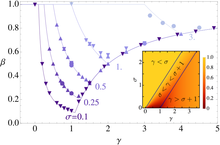
Simulations— The results of our extensive computer simulations of all models are shown in Figs. 1 and 2. We used the gamma distribution for ${P_{D}}(D)$ in (3), and (normal and stretched) exponential, log-normal, and single-point distributions for ${P_{D,{\tau}}}(D,{\tau})$ and ${P_{D,{r}}}(D,{r})$. The exponent $\beta$ was determined for the EMSD by a linear fit of $\log[{\left\langle{x^{2}(t)}\right\rangle}]$ vs $\log(t)$. To analyze the TEMSD, we first determined the diffusivities by a linear fit of the TEMSD vs. the lag at given $T$. We then did a linear fit to a log-log plot of the resulting diffusivities vs. $T$ to get $\beta-1$ in (18). The exponents $\beta$ obtained from the EMSD and TEMSD are in excellent agreement with Table 1. The QRM in regime (II) clearly shows subdiffusion. But at present we have no explanation for $\beta$ in this regime.

To understand why, in the ATTM, we position the particle at the center of a new patch upon hitting a border, recall that a $1$d Brownian path crosses a point infinitely many times before leaving any neighborhood [43]. Now, assume annealed disorder and that the particle enters a new patch at its boundary, as in the QRM. Because a new patch is sampled each time the border is crossed, the particle samples an infinite number of patches during the crossing. In this case, our simulations of the EMSD did not converge with decreasing step length. But the EMSD does converge for the QRM, which visits the same two patches an infinite number of times on crossing a border.

Outlook and Applications— Many questions remain to be addressed. For instance, what is the behavior at the boundaries of the parameter regimes, that is for $\gamma=\sigma$ and $\gamma=\sigma+1$, as well as in regime (II) for the QRM? Regarding dimensions $d>1$: The ATTM and ARM are the same for all $d$, and the EMSD for the quenched CTRW for $d>1$ has the same exponent $\beta$ as the (annealed) CTRW, with logarithmic corrections for $d=2$ [2, 46]. But before analyzing the QRM in $d>1$, a geometry of patches consistent with ${P_{D,{r}}}(D,{r})$ must be found.

Patch models provide an alternative for describing non-ergodic diffusion in biological systems, one that is due to inhomogeneous diffusivity rather than transient trapping. But there are many similarities in the long-time behavior of the CTRW and the patch models. Thus, the main open problem is finding methods to distinguish them, and regime (I) from (II). Promising leads in this direction are studying a first-passage quantity such as the survival time density, or comparing the exponents $\sigma,\,\gamma$ and $\beta$ appearing in our models with those extracted from spatial maps of diffusivity and time-resolved trajectories, or performing a detailed analysis of the models in terms of trajectories with long but finite (i.e., not asymptotically long) duration.