Sequential Detection of an Abrupt Change in a Random Sequence with Unknown Initial State
Abstract
The problem of sequentially detecting an abrupt change in a sequence of independent and identically distributed (IID) random variables is addressed. Whereas previous approaches assume a known probability density function (PDF) at the start of the sequence, the problem addressed is the detection of a single change in distribution among a finite number of known ’equal-energy’ PDFs, but where the initial and final distributions are not known a priori. A Bayesian multiple hypothesis approach is proposed where (i) unlike previous threshold policies, the minimum cost hypothesis is tracked through time, (ii) under an exponential delay-cost function that satisfies an upper bound determined by the distances between hypotheses, the probability of detecting a change from an incorrect initial distribution asymptotically vanishes with time, (iii) computation is recursive and constant per unit time, and (iv) the unknown initial state gives rise to unavoidable incorrect detections that be made to vanish with a constant test threshold with negligibly small effect on correct detection delay for change times beyond a lower bound. Simulations illustrate the analysis and reveal that average delay approaches that of the optimal CUSUM test after an initial transient period determined by an incorrect detection probability constraint.
I Introduction
Let be independent random variables observed sequentially. Each of these random variables are known to follow one of possible known distributions, which are described by probability density functions (PDF) , for , each with finite variance. While observing sequentially, the objective is to determine, as quickly as possible, whether a single change in distribution has occurred at some unknown discrete time without prior knowledge of the initial or final distributions. Generalizations of the standard () quickest detection problem formulation have been considered in [3, 4] but for only limited cases. Specifically, [3] addresses the case where the distribution of the sequence is time-varying after the change time , and [4] considers a random process which is not necessarily IID before and after the change. In both cases, however, the initial PDF is assumed to be known.
Some of change detection’s traditional applications can be found in [5]. An example of more recent interest that features an unknown initial state with arises in cognitive radio, where represents the PDF of noise only, representing the absence of a coherent pilot signal denoting usage of a communication channel, while represents the pilot’s presence in the same background noise [6, 7]. In contrast to previous formulations, the initial state corresponding the PDF at the start of observation is unknown. In addition, conditioned on either or , observations are assumed to be independent.
In the case where the initial state is known, solutions to the problem of detection of a single change in distribution in an independent sequence of random variables can be found in[8, 9, 10, 11], as well as the substantial number of references that can be found in [12]. More recently, the problem of detecting multiple changes in sequences, termed ON-OFF processes has been addressed in [13]. Nevertheless, as in previous approaches, the initial state in [13] is assumed known. It is also worth noting that quickest detection problems yield threshold policies, and the problem of threshold determination to guarantee an exact probability of false alarm has been generally intractable except for a few special cases, e.g., involving a priori Bernoulli PDFs and geometric change time distribution [10, 14, 12].
In the literature there is also what is termed a 2-sided test, i.e., a sequence having two possible final states, as first proposed in [15], analyzed asymptotically and for Normal distributions in[16] and applied to certain problems [17], as well as the detection of changes in drift of Brownian motion [18, 19, 20]. In the latter problem, asymptotic optimality is proven as the frequency of false alarms tends to infinity as well as in an asymptotic minimax sense. In all of the above, although the change or drift itself may be 2-sided, the initial state of the process is assumed completely known. A decentralized version of the 2-sided, known initial-state problem is considered in [21]. However, it has been observed that quickest detection performance is drastically affected if the assumed initial state is incorrect [6].
In previous approaches to one-sided change detection where the initial and final states are known, different performance metrics are used depending on the assumptions about prior information. Bayesian formulations assume that the change time is random with known prior distribution and minimize average detection delay subject to a constraint on the probability of false alarm [14, 10]. Alternatively, an unknown non-random change time is assumed and formulated in a minimax sense in [9], where it has found that the CUSUM procedure by Page [8] minimizes worst-case detection delay subject to an upper bound on the false alarm rate (FAR), or equivalently, a lower bound on the inverse of FAR, known as the average run length (ARL) to false alarm. More recently, the CUSUM procedure has been shown to be optimal in terms of minimizing average delay itself rather than an upper bound [11, 22, 23].
In contrast to the above, the proposed approach to change detection with unknown initial state follows a Bayesian formulation that minimizes expected delay for a specific proposed cost structure. Since initial and final PDFs are unknown, we define incorrect detection of events whenever the initial and/or final states are incorrectly declared. Since information is being gathered over time, we seek a procedure where the probability of incorrect detection of initial state decreases with time. A sufficient condition is if the Bayes’ risks associated with hypotheses with correct initial state converge, while risks corresponding to hypotheses with incorrect initial state become unbounded. In other words, once enough samples are observed, we seek a test with performance that approaches that of a change detector with a known initial state and one of possibly multiple known final states.
This paper extends, generalizes and builds on earlier versions [1] and [2]. A Bayesian change detector is first formulated in [1] under unknown initial state with an exponential delay-cost model, but restricted to two states, i.e, , with only asymptotic behaviour considered, leading to a preliminary version of Theorem 1 in the sequel. The model was improved in [2] to include initial state uncertainty cost, thereby lowering the probability of incorrect initial state of the sequence. Here, we generalize [2], to allow for distributions with equal-energy finite-variance PDFs. In addition, the performance analysis and results are extended, strengthened and more fully described.
While uniform costs and equal priors are sufficient for determining the most likely hypothesis, the causal nature of the problem requires detection delays to be penalized. In Section II, the change detection problem for unknown initial state is therefore formulated under an exponential delay-cost model. Exponential delay cost has been proposed elsewhere [24]. Section II proposes a recursive formulation suitable for problems involving causal (on-line) observation, that implemented by tracking a fixed number of states, which is a consequence of the chosen cost structure. While full joint optimization of the test’s multiple parameters is intractable, Section III presents bounds and tradeoffs that govern suitable parameter choices. Section IV presents Monte Carlo simulations with insights on the performance analysis of Section III, and draws performance comparisons to optimal one-sided quickest detection methods for known initial state[11] [12].
II Change Detection under Unknown Initial State: Bayes Formulation
At time , without knowledge of the starting PDF (of ), a sequence of independent random variables, , is observed. The initial distribution of the sequence is one of possible distributions, which are given by the distinct equal-energy PDFs , for , where for . The sequence may assume possible joint distributions, of which of the sequences, corresponding to no change, are described by the sequence where all , where . The remaining possible sequences, which correspond to each of the possible single distribution changes which occur after the first sample, are described by the sequence where , and the rest of the , where and is the change time. At time , there are change hypotheses as there are possible change times after the first sample and ordered subsets of 2 elements in . Classically, for a fixed number of samples, the detection problem is one of testing a finite number of hypotheses [25] given by . The notation adopted to represent these hypotheses is the following:
| (1) | |||||
In the above, when is selected, there is no detection of a change. If is selected before a change occurs when is true, a false alarm occurs. On the other hand, if is selected and any change has occurred at time there is detection delay. If , for is selected, and the true hypothesis is , for , , , and , then an incorrect detection of final state occurs. If , for is selected, and the true hypothesis does not have as its initial distribution, then an incorrect detection from initial state occurs, regardless of the accuracy of the selected final state or the selected change time .
Suppose for now that time is fixed. To formulate a decision rule to select among the possible hypotheses, we adopt a Bayesian framework. Under equally likely prior probabilities of change time, the Bayesian test minimizes the posterior risk associated with each of the hypotheses. However, when an infinite-duration sequence is causally observed, the number of hypotheses grows with , which results in increasing computation and memory. To alleviate this, a time-recursive version of Bayes risk computation testing is required.
The posterior probabilities for each hypothesis given need to be tracked over time, and we denote the posterior probability that the hypothesis , is true given by for , and similarly the posterior probability that the hypothesis is true given is denoted by . Using Bayes’ Rule,
| (5) |
where is the likelihood of observing given that is true, is the prior probability of , and is the likelihood of observing for the samples received. An equivalent expression to (5) can be written for the posterior probability of the hypothesis given . From the assumed independence conditioned on a certain hypothesis, the likelihood functions in (5) are
| (6) | ||||||
| (7) |
Define hypotheses and , each of which assume the form of either (1) or (II). The proposed Bayes formulation uses cost function , which is the cost of choosing when is true, and the priors
While uniform costs for , for and , and all costs otherwise equal 1 may be used to determine the maximum a posteriori hypothesis at each , alternative cost structures to reflect the problem’s time-sequential nature are more appropriate. Exponential cost has been explored in [24] for change detection problems where the initial state is known, and allow for performance trade offs between average detection delay and false alarm rate.
For change detection under unknown initial state, undesired incorrect detections need to be controlled. Specifically, incorrect detection arising from initial state uncertainty of the sequence occurs if a change from to is declared while is the initial state, for . Hypothesis , for , has its first samples correspond to the initial state. A non-sequential Bayesian test of all -ary possible hypotheses does not associate a cost with uncertainty in initial state, as the likelihood of a certain hypothesis is a function of all observations. The notion of Bayes’ risk for initial state uncertainty for each of the possible change hypotheses is therefore needed in the formulation. Let , , denote the hypothesis with change time , initial state , and prior probability . Using Bayes’ rule, the posterior probabilities are
| (8) |
The likelihood term in (8) factors using independence as
| (9) |
Define wrong initial state cost .
The posterior risk in choosing hypothesis , which corresponds to no change, given , is
| (10) |
The posterior risk in choosing hypothesis ,
| (11) |
The proposed stopping rule, , is to stop at the first such that
| (12) |
From here on equally likely a priori hypotheses, i.e., , and equally likely initial states, i.e., are assumed. To penalize detection delay, false alarm, and incorrect detection, the following cost structure is adopted:
- 1.
Zero Cost: If , .
- 2.
Fixed Costs of False Alarm and Incorrect Final State: If and share initial and final states and corresponds to a change occurring earlier than in , has a fixed cost of false alarm, . Additionally, if and share initial states but not final states, has a fixed cost of incorrect final state, which is also .
- 3.
Exponential Cost of Delay: If and share initial and final states and ’s change time is greater than that of , has the exponential cost of delay, , where is the delay by which lags .
- 4.
Exponential Cost of Incorrect Detection from Initial State: If and have different initial states, has the exponential cost of incorrect detection from initial state, , where is the number of samples in which and are distributed differently.
The cost structure described above is explicitly given by:
Additionally, to penalize initial state uncertainty, for , the following costs are adopted:
In (II)-(II), the constant represents the base of the exponentially increasing cost of delay when the change is in the correct direction from initial state, and represents the base of the exponential cost of incorrect detection. Parameter is the fixed cost of either (i) early correct detection (false alarm), or (ii) incorrect final state. In (II), the parameter serves as the fixed cost of initial state uncertainty.
Applying costs (II) and (II) to (10), Bayes’ rule (5), (8), as well as equally likely priors, the risk associated with choosing hypothesis at time is given by
| (38) |
Using the indepedance of , it can be shown that can be recursively updated from [26]. Similarly, the minimum risks over can also be tracked recursively. Let represent the minimum risk change time at time and let be the minimum risk change time corresponding to time . The minimum risk corresponding to change time is then updated at time according to
| (39) |
In (39), the Bayes risk can be expressed using using costs (II), (II), and (II),
| (40) |
and are updated recursively using the most recent observation . For in (39), the sums from to in (40) are omitted. The detailed recursions can be found in [26]. In short, the minimum-risk hypothesis among the possible change scenarios can be tracked recursively at time with constant time complexity by tracking the minimum of and , a total of of the risks which comprise the state of the detector. While recursive tracking of Bayes risk is possible for more general cost structures, (II)-(II) is shown next to possess desirable properties.
III Cost Parameter Bounds and Tradeoffs
III-A Expected Risks
Recall that cost increases exponentially with the number of observations from the true change time , where the base of the exponents are and . We establish bounds on parameter values to ensure convergence of risks corresponding to hypotheses with the correct initial state and divergence of risks corresponding to hypotheses with incorrect initial states. From the risk expressions (11), (10), (38), (40) and Bayes rule, it can be noted that all risk terms excluding the initial state uncertainty risk terms have the common factor . To establish the parameter bounds, we proceed by finding the expectation of all risks with the factor removed and identify conditions for their convergence or divergence. After that, we show that these conditions extend to expectations of the risk itself.
Using conditional independence, taking expectations of the likelihoods (6) and (7), for , , and we obtain
where denotes expectation with respect to the distribution , and denotes expectation with respect to the hypothesis . Similarly, we get
| (44) | ||||
| (45) | ||||
| (46) |
| (50) | ||||
| (51) | ||||
| (52) |
where constants
| (53) |
We note in Eq. (53),
Lemma 1.
For any set of distinct pdfs such that , and for all .
Proof: See Appendix A.
The and are functions of the length of the test, , and only depend on the known PDFs and and the assumed change time . In the following, these functions serve as common factors when calculating the expected value of the conditional risks. In contrast, the values serve to represent the factor by which the expected value of different likelihoods (III-A)-(46) differ from the functions and .
Multiplying (40) by , averaging over for , and applying (III-A)-(52) yields the likelihood-weighted expected risk for the correct detection hypothesis
| (54) |
which is comprised of geometric series terms, each a function of cost parameters and PDFs. The initial state uncertainty risk in the final term of (54) tends to zero as gets large, and thus has vanishing influence on test behaviour for large change times.
III-B Parameter Choices for Large Change Times
To provide insight into the time sequential notions of correct and incorrect detection, we first focus on the large change-time regime where after observing for a long time, the change has yet to occur. That is, in this subsection, we assume that while remains finite, and thereby avoid situations where an incorrect detection corresponds to a vanishingly small transient initial state, an assumption consistent with the chosen cost structure. Observing (54), every term involving an exponential cost is a product of terms of the form or for . If we choose parameters and to be such that each of these individual terms is less than one, then each of the geometric series terms with exponential costs will asymptotically converge, and finite shifts in change times in (54) do not affect convergence. The terms which include the fixed cost, , will converge to a finite value for any . Thus, under the large change-time regime, the expected risk Eq. (54) can be shown to converge by choosing , , , and , where
| (55) |
We note that by Lemma 1 and we recall that and are assumed in the cost function definition. It can similarly be shown that choosing will result in the expected risks for hypotheses with incorrect initial state diverging asymptotically by considering for . The process of calculating for is the same as was used to find Eq. (54), but in this case several geometric series terms will diverge exponentially with base as increases.
Next, we need to establish
Lemma 2.
Assume that each has finite variance. For , if the expected value of the likelihood-weighted risk converges or diverges as gets large, will also converge or diverge, respectively.
Proof: See Appendix B.
We then have
Theorem 1.
Under the conditions
| (56) |
, and , the probability of incorrect detection of the proposed procedure (12) converges to zero asymptotically for the large change-time regime as the number of observations gets large.
Proof.
According to Lemma 2, for establishing convergence or divergence, we may consider the average risks of the form (54). Applying the conditions (56) to (54), at least one of the expected risks corresponding to correct detection converges to a steady state. This means that the minimum Bayes risk of correct detection in (12) must be bounded, and denote its value by . Consider the random variable , where is the risk associated with choosing , a hypothesis with incorrect initial state, and denotes . It follows from (56) that is a diverging incorrect detection hypothesis. Applying Markov’s inequality,
| (57) |
for any . Since under the large change-time regime, the expectation on the right hand side vanishes as for any finite . As any positive probability on the left-hand side represents the probability that is the minimum risk hypothesis, we see that the incorrect detection probability vanishes to zero. ∎
Remark 1.
Risks for hypotheses with incorrect initial state will stay large under the large change-time regime after a change occurs. In fact, a larger value of causes incorrect-detection risks to diverge more quickly, reducing the probability of incorrect detection. In addition, the time spent in an initial state where incorrect-detection risks are small enough to incur an incorrect detection decrease as increases.
III-C Parameter Choices for Initial State Uncertainty due to Small Change Times
Theorem 1 is conditioned on the large change-time regime, i.e., each of the recursively tracked minimum-risk change times growing with before a change occurs, and is presented to justify the exponential cost structure. It is worth noting, however, that the assumption of a large change-time regime is not valid in all situations. If the parameters and are selected according to (56), then the recursively tracked change times for risks corresponding to hypotheses with incorrect initial state should stay small since the algorithm identifies the minimum-risk hypothesis corresponding to change in each direction. Consequently, if the recursively tracked change time is small, then the asymptotic analysis leading to Theorem 1 does not apply. Additionally, for small change times the exponential cost structure does not always associate a large cost with incorrect detection, which is obviously undesirable. This motivates the use of the initial state uncertainty cost, , which provides a mechanism to address the inherently large probability of incorrect detection for small change times.
For any particular risk corresponding to change, when the recursively tracked time is small, only a small number of samples can be used to determine the initial state of the sequence . The cost parameter mitigates risk caused by early change-time hypotheses to prevent incorrect detections caused by this initial state uncertainty. As the number of initial state samples increases, the risk vanishes for correct-sided risks corresponding to change and remains large for incorrect-sided risks. Before we proceed, we define and as the Kullback-Leibler divergence between PDFs and . The initial state uncertainty risk associated with the proposed procedure, (12), is shown to have the following property:
Theorem 2.
Under the conditions (56) and , the following properties hold:
(i) the probability of incorrect detection of the proposed test can be made arbitrarily small by using a sufficiently large threshold ,
(ii) for change times
| (58) |
for some , where is a finite constant, initial state uncertainty increases the expected correct detection delay as , and
Proof.
See Appendix B. ∎
Remark 2.
The choice of parameter governs the trade off of incorrect detection probability against the ability to detect changes occurring prior to some minimum detectable change time.
In Theorem 2, a value of the minimum change time (58) is used to showcase performance trade-offs; however, the value of this minimum change time is not useful for practical test design purposes since it is simply the average number of samples from the initial state required for the initial state uncertainty risk to vanish among other risk terms, which is expressed by Eq. (79) in Appendix B. Rather, it is more useful to find the smallest change time satisfying
| (60) |
for some chosen , which can be obtained from Eq. (81) in Appendix B. This corresponds to the minimum change time for initial state uncertainty to affect average detection delay with probability . Unfortunately, computation of the minimum satisfying (60) in general is difficult as it requires the cumulative distribution function of conditioned on . To avoid this, in Section IV-C the increase in average detection delay due to initial state uncertainty risk is quantified instead.
III-D Delay and False Alarm
It is worth further investigating the correct-sided risks for finite under the conditions (56). Interpreting Eq. (54) and Eq. (85), Appendix B, it can be noted that increasing parameter for fixed and serves as a mechanism to lower both probability of false alarm and probability of incorrect detection. Under correct detection hypotheses, in view of the terms including cost parameter in Eq. (54) and , false alarms are controlled by the added risk (which incurs added delay). Therefore, increasing while using values of and that satisfy Theorem 1 can be used to achieve additional performance tradeoffs of decreased detection error probabilities at the expense of delay.
Nevertheless, from Theorem 2, there exists an irreducible minimum change time required for correct-sided initial state uncertainty risk to vanish, and it can be expressed directly in terms of the cost parameters and distributions. Since in (58) is not a function of cost parameter , this minimum change time only increases logarithmically in , which indicates insensitivity to delay penalty. Taking (76), Appendix B, into account, we conclude that increasing to reduce the probability of incorrect detection would incur only a modest effect on delay in correct detection.
IV Simulations and Numerical Results
IV-A Simulation Description and Parameter Selection
To illustrate the performance of the proposed test and its finite sample properties, i.e., Theorem 2, Monte Carlo simulations were performed when initial state uncertainty cost is changed. We use , which is sufficiently general for this purpose. An example featuring can be found in [26]. Here, consider detecting a change in the mean of Gaussian PDF, to , i.e.,
where is the mean shift after the change in distribution and is the variance. Define signal-to-noise ratio as . From (IV-A), (53) and (55) we obtain . Using an SNR of yields . To satisfy conditions (56) for Theorem 1, we choose parameter values and to associate a larger cost with incorrect detection than detection delay. A cost of false alarm is chosen, using the trade-off between average detection delay and false alarm rate discussed in Section III-D, to achieve a false alarm rate of approximately 0.05 when the change time is and the initial state uncertainty cost is . To illustrate how initial state uncertainty cost influences probability of incorrect detection of initial state and average detection delay, initial state uncertainty cost is varied from to , and for each value of , the test performance is simulated using Monte Carlo trials for changes times varying from 5 to 100 in increments of 5. For each trial, the initial state of the sequence is chosen randomly, and assumes either or with equal probability. The results are presented in Section IV-B. In Section IV-C, the performance bound on the probability of incorrect detection and the average detection delay presented in Theorem 2 is compared with observed results and trends. Finally, Section IV-D provides summary discussion.
An obvious comparison point is to use a fixed sample size (FSS) hypothesis test (HT) to detect the initial state of the observed sequence. Once the initial state is identified, a traditional change detection scheme, i.e., one that assumes knowledge of the initial state, such as Page’s CUSUM, could be used to assess detection delay. Since choosing the length of the FSS HT requires knowledge of the change time, which is unrealizable, this is only used as a benchmark; in Section IV-B, the incorrect initial state detection probability of the FSS HT and the average detection delay and false alarm rate of CUSUM are presented alongside that of the proposed change detection scheme. For the FSS HT, the incorrect detection rate shown assumes a known change time and chosen to be the change time minus one. For a meaningful comparison, a CUSUM threshold of was chosen achieve approximately the same ARL to false alarm as the proposed scheme with the above parameter values.
IV-B Monte Carlo Simulation Results
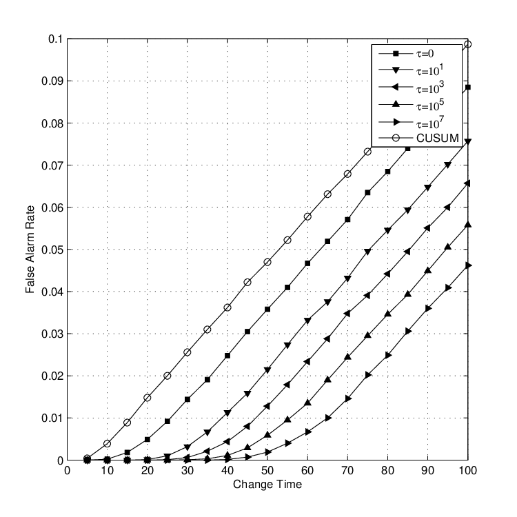
For the PDFs (IV-A) and parameter values selected in Section IV-A, Figures 1, 2, and 3 plot average detection delays, incorrect detection rates, and false alarm rates, respectively, achieved by the proposed change detection scheme in the Monte Carlo simulation.
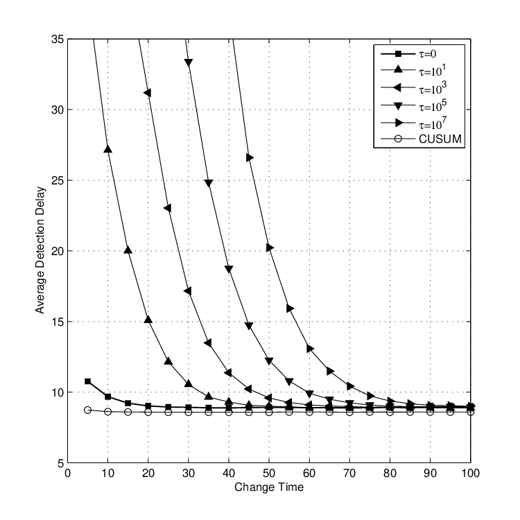

From Figure 1 it is clear that average detection delay increases for any given change time when the initial state uncertainty cost, , is increased, which is consistent with Theorem 2. When the change time is small, the average detection delay of the test for all is much larger than for . However, as the change time increases, the average detection delay becomes insensitive to cost as expected. Additionally, it can be noted that the average detection delay of the proposed change detection scheme after an initial transient period is only slightly greater than that of CUSUM, which is known to be average-delay-optimal for known initial state and FAR constraint. The average detection delay of CUSUM is measured to be 8.586, while that of proposed scheme once the initial state is established is 8.903, which is only 3.69 % larger.
Observing Figure 2, it is clear that each value of achieve a minimum probability of incorrect detection, which decreases as is increased. At the same time, increasing also increases the minimum change time for when this minimum incorrect detection rate occurs. These results are consistent with Theorem 2. For example, for , a minimum incorrect detection rate of approximately is achieved and it reaches this minimum at a change time of approximately sample 45. When is used, a much larger incorrect detection rate floor of approximately is achieved earlier, by sample 15. These results clearly illustrate the trade-off between the probability of incorrect detection of initial state and the test’s ability to detect early change times. Comparing the proposed change detection scheme’s incorrect initial state detection rate to that of the FSS HT, it can be observed that at for each change time there is a value of for the proposed test that achieves a lower incorrect detection rate than the FSS HT. Not surprisingly, no value of is universally better than the FSS HT which requires initial state knowledge.
Figure 3 shows the false alarm rates achieved by the proposed change detection scheme for different values of . It is clear that after an initial transient period during which the initial state is established, false alarm rate increases linearly with change time. This is consistent with Theorem 2, that specifies how the initial transient period increases with . It can also be noted that, following the initial transient behaviour, the rate at which false alarm rate increases with change time is approximately invariant with , which indicates that the parameter has a negligible effect on the ARL to false alarm. Recalling that an increase in average detection delay caused by initial state uncertainty risk vanishes following initial transient behaviour of the test, we conclude that the initial state uncertainty risk does not affect the trade-off between the probability of false alarm and average detection delay. Finally, it can be noted that the rate at which the false alarm rates increase for both CUSUM and the proposed change detector are approximately the same. This was intended, as it was desired for both tests to have approximately the same ARL to false alarm for benchmarking purposes. It should be noted that Figure 3 presents the false alarm rate of CUSUM under the assumption that the initial and final states are known. To compare the false alarm rates of CUSUM to that of the proposed change detection scheme, the duration and the outcome of the FSS HT would need to be considered. The inclusion of false alarm rates for CUSUM in Figure 3 is there to justify the selected CUSUM threshold of for the comparison.
IV-C Analysis of Simulation Results
We next compare the results presented in Figures 1 and 2 with the performance bounds presented in the proof of Theorem 2. As pointed out previously from Figure 2, once the initial state of the sequence is observed for long enough, each value of reaches a minimum probability of incorrect detection from initial state, and this minimum decreases as is increased. Eq. (77) in Appendix C shown below is an upper bound on the probability of incorrect detection from initial state. For with and defined as in (IV-A), . Since the PDFs are symmetric about , the performance of the test is the same regardless of whether or is the initial state. Without loss of generality we proceed by using (77) and to calculate
| (63) |
Using the given PDFs,
| (64) |
We found the value of to be approximately 1.05 by taking an average of over for true over Monte Carlo trials. With this value of and (64), upper bounds (63) can be found for a given value of using two 1-dimensional searches. For values of of , , , and , the probability of incorrect detection upper bounds were found to be , , , and respectively. Comparing values with Figure 2, (63) is a loose upper bound: incorrect detection probabilities for and are smaller than their respective upper bounds by factors of approximately and respectively. This is expected, as the formulation of (63) considers only initial state uncertainty cost , and ignores the exponential costs used to prevent incorrect detections.
In Theorem 2, a minimum change time for initial state uncertainty risk to negligibly increase delay was identified. Eq. (60) is the probability that the initial state uncertainty risk is larger than expected risk given a change time , which incurs additional expected delay. It is desired to find the smallest such that the probability (60) is smaller than some small value . We compute
| (65) |
Noting that is distributed according to , each of the ’s in (65) are IID , (65) is Gaussian with mean and variance . Thus, (60) becomes
| (66) |
For , we obtain by calculating the average values of over over Monte Carlo trials. For values of of , , , and , Eq. (66) yields minimum change times of 40.8, 59.2, 74.09, and 88.2, respectively. Interpolating linearly between data points of the average detection delay plot in Figure 1, the minimum change times for values of of , , and yield average detection delays of 9.261, 9.123, 9.115 and 9.106, respectively. The change detector for achieves an average detection delay of 8.90 over change times of 20 through 100, which is only slightly smaller, within , , , and , respectively, of the above calculated minimum average detection delays. Additionally, from Figure 2 it can be observed that, for each value of , the incorrect detection rate achieved matches that calculated using (66), i.e., (60) identifies the duration of the initial transient period of the test.
IV-D Discussion
The above Monte Carlo simulations illustrate performance bounds and trade-offs presented in Theorem 2. Specifically, the initial state uncertainty cost can be chosen to trade off probability of incorrect detection from initial state according to a minimum change time and without appreciable average detection delay penalty. Furthermore, once this minimum value of change time has been reached, initial state uncertainty risk decreases asymptotically to zero and thus does not affect the trade-off between the probability of false alarm and the average detection delay.
In summary, while joint optimization of parameter values , , and is complicated, we have instead shown that after a controllable initial transient period, the proposed change detection scheme can achieve detection delays close to that of CUSUM, which is optimal for the case where the initial state is known. Further, initial state uncertainty was considered and it was found that that there is a range of change times where the proposed change detector outperforms FSS HT, which assumes full knowledge of the change time, in the form of the correct initial state detection probability. This can be attributed to the proposed change detector recursively tracking the minimum risk change time for each state pair , whereas the FSS HT ignores the temporal behaviour of observed samples prior to the change.
V Conclusions and Future Work
A Bayesian change detection scheme has been proposed with exponential incorrect detection cost structure for a sequence of independent random variables that is known to start at one of equally likely possible PDFs and end at another. Suitable parameter choices have been analytically shown to trade off the probability of incorrectly identifying the initial PDF against the test’s false alarm probability and average detection delay and are illustrated by Monte Carlo simulation. Additionally, the simulations reveal that the proposed change detection scheme achieves an average detection delay close to that of the optimal change detector for the same ARL to false alarm and where the initial state is known. The analysis is restricted to the case where each of the PDFs have equal energy, which includes the case of different shifts in the mean. Generalizing the results to consider broader classes of PDFs is a subject of future investigation.
VI Appendix
VI-A Proof of Lemma 1:
Proof.
In (53), both numerator and denominator take the form
| (67) |
For ,
| (68) |
where the Cauchy-Schwarz inequality is used, and and since both and are non-negative functions. The inequality is strict since and are distinct and not linearly dependent. By letting , it follows straightforwardly that . Similarly, , noting that . ∎
VI-B Proof of Lemma 2:
Proof.
Consider
| (69) | |||||
using the Cauchy-Schwarz inequality, and is finite by assumption that the PDFs have finite variance. Applying Jensen’s inequality
| (70) |
In (70), is finite for any realization and thus the left and right hand sides of (70) are a finite distance apart. Applying (70) to (69) yields
| (71) |
and we conclude that is a finite distance from .
can be calculated similarly to Eq. (54) using (III-A)-(52) to be a product of and a sum of geometric series terms, which along with Lemma 1, can be shown to converge, and thus is a finite distance from . Taking expectation over , we conclude that is finite. In a similar manner, using (71) while taking expectation over for and , diverges, and thus , a finite distance away, also diverges. ∎
VI-C Proof of Theorem 2:
Proof.
Part (i): From Theorem 1, converges to a finite value. For incorrect detection at time , there exists , for , , and when is true.
Let . Since the parameter values and follow (56) and , . Using (11) under , the all- hypothesis, an incorrect detection may only arise from incorrect initial state when
| (72) | ||||
| (73) |
Eq. (73) follows from (72) since the omitted term (which only exists for ) is strictly less than zero. Let and . Since the sequence is IID, so is . For any , the Chernoff bound yields
| (74) |
where is the moment generating function of and
| (75) | ||||
| (76) |
using recursively tracked change time, , and minimizing over .
The numerator of Eq. (76) is positive for , any pair and , and any . Thus,
| (77) |
By choosing sufficiently large, Part (i) holds.
Part (ii):
Denote the risk of excluding initial state uncertainty risk as
| (78) |
For the initial state uncertainty risk to vanish among all correct-sided risks, we require
| (79) |
where . Equivalently,
| (80) |
Therefore,
| (81) |
Taking the expectation of (81) conditioned on yields
| (82) |
where
| (83) |
Without loss of generality, we assume that the recursively tracked change time is the actual change time. Detection delay is the difference after stopping to detect a change in the correct direction. Ignoring the influence of incorrect-sided risks, stopping occurs when
| (84) |
The expectation of the right side of (84) is given by (54), and has been shown to converge to a finite value as gets large. Taking the expectation of the left side of (84),
| (85) |
which contains terms that increase exponentially with base following the change at time .
The average detection delay is the smallest satisfying the expectation of (84) conditioned on . It can be shown that for , , and observing (54), . For fixed , the risk associated with initial state uncertainty is constant as increases. From (85), has terms which increase as . Since average detection delay is the amount of time after for to surpass , on average, the threshold increases detection delay by
| (86) |
where is determined by the largest value of satisfying (56). Thus, average detection delay increases , establishing (ii).
Part (iii): Additionally, under (59), initial state uncertainty risk increases average detection delay, and it can be shown that . Again, considering the increase in average detection delay from initial state uncertainty risk, under (59), the numerator of (86) approaches the constant . Thus, delay from initial state uncertainty increases as . ∎
References
- [1] J. Falt and S. Blostein, “A Bayesian approach to two-sided quickest change detection,” in IEEE ISIT, 2014, pp. 736–740.
- [2] ——, “Two-sided change detection under unknown initial state,” in CISS, 2016, pp. 418–423.
- [3] S. Blostein, “Quickest detection of a time-varying change in distribution,” IEEE Trans. Information Theory, vol. 37, no. 4, pp. 1116–1122, 1991.
- [4] G. Moustakides, “Quickest detection of abrupt changes for a class of random processes,” IEEE Trans. Information Theory, vol. 44, no. 5, pp. 1965–1968, 1998.
- [5] M. Basseville and I. Nikiforov, Detection of Abrupt Changes: Theory and Application. Prentice-Hall, 1993.
- [6] J. K. Liang and S. Blostein, “Performance evaluation of multiband multi-sensor spectrum sensing systems,” in IEEE GLOBECOM, 2011, pp. 1002–1007.
- [7] C. Stevenson, G. Chouinard, Z. Lei, W. Hu, S. Shellhammer, and W. Caldwell, “IEEE 802.22: The first cognitive radio wireless regional area network standard,” IEEE Communications Magazine, vol. 47, no. 1, pp. 130–138, Jan. 2009.
- [8] E. S. Page, “Continuous inspection schemes,” Biometrika, vol. 41, pp. 100–115, June 1954.
- [9] G. Lorden, “Procedures for reacting to a change in distribution,” Ann. Statist., vol. 42, no. 6, pp. 1897–1908, 1971.
- [10] A. N. Shiryaev, Optimal Stopping Rules. Springer, 1978.
- [11] G. V. Moustakides, “Optimal stopping times for detecting changes in distributions,” Ann. Statist., vol. 14, no. 4, pp. 1379–1387, 1986.
- [12] H. V. Poor and O. Hadjiliadis, Quickest Detection. Cambridge University Press, 2008.
- [13] Q. Zhao and J. Ye, “Quickest detection in multiple on-off processes,” IEEE Trans. Signal Proc., vol. 58, no. 12, pp. 5994–6006, Dec. 2010.
- [14] A. Shiryaev, “On optimum methods in quickest detection problems,” Theory Prob. App., vol. 13, no. 1, pp. 22–46, 1963.
- [15] G. Barnard, “Control charts and stochastic processes,” J. Roy. Statistical Soc., vol. 21, pp. 239–271, 1959.
- [16] V. Dragalin, “The design and analysis of 2-CUSUM procedure,” Communications in Statistics - Simul. Comput., vol. 26, no. 1, pp. 67–81, 1997.
- [17] T. Barnett, D. Pierce, and R. Schnur, “Detection of anthropogenic climate change in the world’s oceans,” Science, vol. 292, no. 5515, pp. 270–274, 2001.
- [18] O. Hadjiliadis, “Optimality of the 2-CUSUM drift equalizer rules for detecting two-sided alternatives in the brownian motion model,” J. Applied Prob., vol. 42, no. 4, pp. 1183–1193, 2005.
- [19] O. Hadjiliadis and G. Moustakides, “Optimal and asymptotically optimal CUSUM rules for change point detection in the brownian motion model with multiple alternatives,” Theory Prob. App., vol. 50, no. 1, pp. 131–144, 2006.
- [20] O. Hadjiliadis and H. Poor, “On the best 2-CUSUM stopping rule for quickest detection of two-sided alternatives in a brownian motion model,” Theory Prob. App., vol. 53, no. 3, pp. 610–622, 2008.
- [21] S. Zarrin and T. J. Lim, “Composite hypothesis testing for cooperative spectrum sensing in cognitive radio,” in IEEE ICC, 2009, pp. 1–5.
- [22] M. Pollak, “Optimal detection of a change in distribution,” Ann. Statist., vol. 13, no. 1, pp. 206–227, 1985.
- [23] Y. Ritov, “Decision theoretic optimality of the CUSUM procedure,” Ann. Statist., vol. 18, no. 3, pp. 1464–1469, 1990.
- [24] H. Poor, “Quickest detection with exponential penalty for delay,” Ann. Statist., vol. 26, no. 1, pp. 2179–2205, 1998.
- [25] H. V. Poor, An Introduction to Signal Detection and Estimation. Springer-Verlag, 1994.
- [26] J. Falt, “Bayesian detection of a change in a random sequence with unknown initial and final distributions,” Master’s thesis, Queen’s University, 2017.