A Microkernel Architecture
for Constraint Programming
Abstract
This paper presents a microkernel architecture for constraint programming organized around a number of small number of core functionalities and minimal interfaces. The architecture contrasts with the monolithic nature of many implementations. Experimental results indicate that the software engineering benefits are not incompatible with runtime efficiency.
1 Introduction
Over the years, the constraint programming community has built and experimented with a variety of system design and implementation Historically, solvers were embedded in logic programming languages, CHIP [3], CLP(R) [11], and Prolog III [2] being prime examples. Later solvers were packaged as libraries hosted in traditional object-oriented and imperative languages. Examples abound starting with Ilog Solver [10], Gecode [22] and Minion [8] for C++ and Choco [12] or JacOP [13] for Java (to name just a few). The success of algebraic modeling languages in the mathematical programming community as well as the desire to not be constrained by the host language prompted advances in domain-specific languages, a trend examplified by Oz/Mozart [23], Opl [24], Salsa [14], and Comet [25] for instance. In all cases, the traditional constraint-programming capabilities are exposed by an API capturing the mantra
However, in these implementations, the solver is delivered as a monolithic piece of software incorporating key notions such as variables, constraints, events, propagation protocols, propagators, and search support. Perhaps even more strikingly, propagation engines include provisions to deal with decisions variables of many different types (e.g., int,float,set), possibly replicating the APIs for each variant. Orthogonal features (e.g., the support for AC-5, views, and advisors) further contribute to complexity as APIs must be duplicated to transmit additional information to the propagators when events of specific classes occur. While conceptually simple, this approach does not scale very well. Consider the Comet API shown in Figure 1. It blends support for AC-3, AC-5, and the ability to convey the index of a variable to a propagator along with two types of decision variables. The protocol AC5Constraint<CP> in lines 1–13 only captures the methods that a propagator supporting AC-5 could implement. Line 9, for instance, specifies method valRemoveIdx which is called whenever variable appearing at index in some array has lost value . Similarly, the integer variable VarInt<CP> offers one registration method for each class of events that the variable is susceptible to raise. The net result is a large APIs encompassing the union of core capabilities for all variable types and event classes.
This paper examines a possible alternative to such a design: It describes the microkernel of the Objective-CP [28] system, a new constraint programming system that refines the core mantra to
Objective-CP isolates all the responsibilities associated with model manipulation, rewriting, specialization and reformulation in the modeling component. This factorizes key capabilities that are reusable by multiple solvers and promotes the idea of model combinators described in [5]. Objective-CP also supports search facilities through a technology-neutral search library featuring combinators and a seamless symbiosis with the host language, i.e., Objective-C. The search library [29] makes it possible to specify and execute complex search procedures with minimal effort and delivers competitive performance. The Objective-CP constraint-programming solver embraces the idea of a microkernel architecture inspired by recent develoments in operating systems. The constraint engine features a number of small components with parsimonious interfaces. Microkernel architectures have become very popular in operating systems as they favor extensibility and maintenance, and make proofs of correctness easier. The constraint-programming engine underlying Objective-CP delivers a truly modular architecture where variables, domains, and constraints all remain completely external to the microkernel. Each computational domain (e.g., booleans, reals, integers, sets) becomes a service on top of the microkernel, providing the necessary infrastructure for propagation-driven inferencing. In particular the microkernel isolates the propagation logic and events protocols from the variables and constraint definitions. This architecture is therefore a departure from the monolithic organization prevalent in modern solvers. It is designed to encourage the construction of separate libraries each featuring different domains, variable representation (e.g., finite-domains, intervals, sets, MDDs) and constraints.
The rest of the paper is organized as follows. Section 2 provides a brief overview of Objective-CP and the vision for the system. Section 3 covers the functionalities of the microkernel. Section 4 discusses how to use the microkernel to implement a finite-domain solver. Section 5 offers empirical evidence of the platform capabilities and Section 6 concludes the paper.
2 Overview of Objective-CP
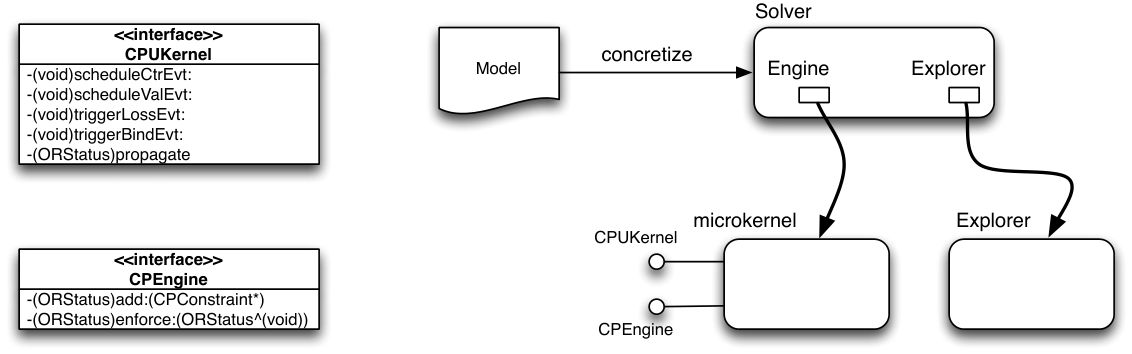
The design of Objective-CP takes the view that
Optimization Program = Model + Search + Solver
or, in other words, that an optimization program consits of a model, a search, and an underlying solver. The overall architecture is illustrated in Figure 2 where a model is concretized into a solver. The solver is the composition of an engine (responsible for the representation of constraint, variables, and the inferencing) and an explorer (responsible for technology-neutral search capabilities). The kernel itself implements the two interfaces shown on the left-hand side to drive the propagation (the CPUKernel) and to register constraints and variables (the Engine).
2.1 The Vision underlying Objective-CP
Models
Models are first-class objects in Objective-CP. They follow the style of constraint programming and are solver-independent. This allows for easy experimentation with different technologies and smooth hybridizations [5, 6]. Models can be transformed and refined through a sequence of operators that, for instance, replace algebraic equations with lower-level elementary constraints. The final model is then concretized into a specific solver to obtain an optimization program, (e.g., a constraint program or a mixed-integer program). Given a model , a sequence of model operators , and a concretization function for a solver technology , the application
derives a concrete program based on technology . The resulting program can be solved using a black-box search or a dedicated search procedure expressed in terms of the model variables present in .
Search
Search procedures in Objective-CP are specified in terms of high-level nondeterministic constructs, search combinators, and node selection strategies, merging the benefits of search controllers and continuations [27] on the one hand and compositional combinators (e.g., [21]) on the other hand. The search language is generic and independent of the underlying solver. Naturally, search procedures call the underlying engine for adding constraints, binding variables, and querying the search state.
Engine
The underlying engines can leverage any combinatorial optimization technology ranging from linear programming and integer programming to constraint programming and constraint-based local search. The role of the engine is to isolate the state representation and inferencing capabilities. This paper focuses on a microkernel architecture for the inference engine focused on “traditional” (finite-domain) constraint programming.
2.2 First-Order Functions
Objective-CP leans heavily on its host language (Objective-C) to implement its capabilities. In particular, it relies on closures and first-order functions. In Objective-C, it is straightforward to turn any C block into a first-order function. For instance, the fragment
uses an Objective-C block to produce a first-order function capable of printing an object (). The first-order function is then used to visit a set and print its entire content. The syntax of Objective-C block is reminiscent of the syntax for function pointers in : The caret symbol indicates a block creation.
2.3 An Objective-CP Primer
This section is a brief primer to Objective-CP. Consider the Steel Mill Slab problem as an example. An abridged11 1 The data reading part of the program is omitted for brevity. Objective-CP implementation is shown in Figure 3. In this program, line 1 first creates a model , while lines 5 and 6 create two decision variable arrays and to represent the slab assignment and the load of each slab. Lines 8–11 state the model constraints, i.e., a global packing constraint and a coloring constraint for each slab, and the objective function (line 11) which minimizes the total loss. The model is not specific to constraint programming and Line 13 transforms and concretizes this high-level model into a constraint program. While is clearly constructed with algebraic expressions, the microkernel underlying the CP engine operates on a rewriting of the model featuring exclusively low-level and global constraints. To be more precise, line 13 is equivalent to
where is a flattening operator that creates a new model based on in which all relations and expressions have been replaced by basic constraints. is a concretization function that associates a concrete variable with each modeling variable in , as well as a propagator with every modeling constraint in . The concretized model is then loaded into the engine of a constraint-programming solver. Finally, lines 15–25 implement the search and rely on the tryall: combinator to specify the non-deterministic choices. It is worth noticing how Objective-CP blends the control primitive of the host language with search combinators in a completely transparent and fully compositional way. From an Objective-CP end-user standpoint, the entire search is expressed in terms of the decision variables from . Method calls such as label:with: and diff:with: are exclusively manipulating model variables, yet they are automatically recasted in term of concrete variables and delegated to the underlying engine. Indeed, the call in the closure on line 21 becomes
where the abstract constraint slab[i] == s is flattened with and concretized with before being transmitted to the underlying engine.
2.4 A Solver Interface
A solver is the composition of an explorer responsible for the search and an engine responsible for inferencing. The engine implements two distinct interfaces. The engine interface is the solver-facing part of Objective-CP needed for concretizing models: It offers the necessary capabilities to register variables, constraints, and objective functions. The microkernel interface is used by system developers when building new propagators: It offers the functionalities for propagation-related activities such as the dispatching of events.
The Engine
The interface shown in Figure 4 is the visible tip of the iceberg for microkernel users. It is the API needed to load constraints and objective functions. It offers only three methods to register a concrete constraint over concrete variables (line 2); to set the objective function via the setObjective: method (line 3); and to execute an arbitrary closure and propagate its effects with the enforce: method (line 4). The closure passed to enforce: returns a status (i.e., an element in the set ) to report the propagation outcome.
Constraints
The CPConstraint protocol used by the engine is shown below
It only requires that a constraint carries a unique identifier and responds to a post request. Naturally, constraints have additional methods but these are not mandated by the microkernel.
Objective
The ORObjective protocol is shown below alongside a protocol to describe the value of an objective function.
At its most abstract level, one can query an objective to retrieve its current value represented as an abstract object as well. Note how ORObjectiveValue instances can be compared to pick the best value. Naturally, one should only compare objective values issued by the same objective function, so that the optimization direction is correctly taken into account. For instance, a call to best: on an objective value receiving an objective value returns the best overall objective value. If the objective function was a minimization over the real, the returned result encapsulates a value ranging over the reals and retains the knowledge that it is coming from a minimization.
3 The Microkernel Architecture
The purpose of the microkernel is to act as a relay for messages pertaining to the propagation of constraints. The key challenge is to design a small set of capabilities to suppot variables, constraints, and propagation techniques of different forms. While it is always possible to define a kernel offering the union of all the required capabilities, the approach does not scale and is truly intrusive when designing new classes of constraints with different messaging requirements as illustrated in the introductory example with the Comet API in Figure 1.
The constraint-programming microkernel of Objective-CP presents an alternative design based on a minimalistic API with two capabilities:
- •
scheduling events
- •
propagating events.
The API of the microkernel per se is shown in Figure 5. Line 2 descibes the method for scheduling constraint events, Line 3 the method for scheduling value events, Line 4 the method for scheduling all triggers associated with a value loss, and line 5 the method for scheduling all triggers associated with a value binding. Finally, line 6 is the method needed to trigger the inferencing. These APIs only require a handful of other protocols that embody the concept of event lists and maps. Namely, they reference CPClosureEvent, CPValueEvent, and CPTriggerMap. In the following section, responding to events is best understood as executing an arbitrary piece of code represented by a function. The exact nature of the response is discussed in Section 3.3.
3.1 Propagation Preliminaries
Events
The concept of event is the cornerstone of the microkernel. Events are the vehicle of choice to relay information and takes a very abstract form that is independent of the nature of the variables involved. In this paper, events are closures in a functional-programming sense. Namely, they are blocks of code that capture the computational state at the time of their definition and are wrapped in a first-order function (of type ) that can be saved, called, or passed to other functions.
Priority Space
The microkernel supports event priorities, using a range of numerical values , where is the highest priority and is the lowest. Two priorities in this range have special statuses. Priority is always dispatched regardless of the outcome of the propagation, i.e., even in case of a failure. Priority is reserved for value-driven events. The remaining priorities () are available for general use. The existence of a special priority may sound surprising at first. However, it is the ideal vehicle to implement key functionalities in a non-intrusive way. To illustrate, simply consider black-box search heuristics such as Ibs and Abs. Both necessitate that, at the end of a propagation cycle and irrespective of the outcome, variable statistics be updated for every variable involved in the fixpoint (e.g., for Abs search, one must update the activity of the variables that participated in the fixpoint computation). In a traditional kernel, such a support requires the instrumentation of the solver to invoke, at the end of the fixpoint, the code fragment responsible for updating those statistics. An always priority (i.e., priority 0) solves this problem. Indeed, one can simply attach a daemon with every variable and schedule it at priority 0. When the daemon runs at the end of the propagation, it updates the statistics stored in the implementation of Ibs or Abs. Priority 0 can also be useful for implementing visualizations where some redraw must be done regardless of the propagation outcome and are driven by the variables touched during the propagation.
Queues
The microkernel of Objective-CP is responsible for dispatching events arising as a result of the propagation of constraints. To this end, it relies on an array of queues in which refers to a queue at priority .
3.2 The Propagation Engine
While an OS microkernel is tasked with continuously dispatching messages to the processes it manages, the Objective-CP microkernel only dispatches accumulated messages at specific points during the execution. This section is concerned with the dispatching process alone and it presents the implementation of the propagate method of Figure 5.
The Propagation Loop
The dispatching algorithm is shown in Figure 6: It processes each non-empty queue in turn from the highest () to the lowest () priority. Line 5 finds the index of the highest priority queue with some events. Lines 6–9 pick the first highest priority event, dispatch it (line 7) and carry on until which indicates that all queues in the range are empty. Finally, lines 12–13 unconditionally execute all the events held in . As is customary, the dispatching of messages may schedule additional events that will be handled during this cycle. Since individual events are represented by closures of the form , dispatching an event is modeled by a simple instruction that executes closure .
Handling Inconsistencies
Producing an elegant propagator implementation can be a challenge with modern constraint-programming solvers. Variable updates triggered by a propagator can lead to domain wipe-outs, revealing an inconsistent computation state (aka a failure). Programmers are therefore expected to lace the propagator implementation with failure checks and to abort the propagation when a failure is encountered. Each propagator must also return a suitable status, indicating whether the propagation failed.
Objective-CP relies on an alternative design and relies on native
exceptions to report failures. The block spanning lines 4–14 in
Figure 6 invokes closures that capture the logic of
propagators and can potentially induce failures. It is therefore
captured in a closure and passed alongside a second closure (lines
16–18) to the utility function tryfail. The semantics of tryfail(,) is similar to a try-catch block, i.e., it can
be understood as the rewriting:
that executes and transfers control to in case a failure exception is raised.
Exceptions, however, are meant to alter the control flow in rare and exceptional conditions. As a result, the implementation of exceptions, e.g., the libunwind library in C++, induces a negligible overhead when executing try blocks but incurs a more significant cost when throwing and unwinding the stack to catch and handle the exception. Failures in constraint programming are rather frequent however and such an implementation would produce non-negligible slowdowns.
To remedy this potential limitation, Objective-CP implements a low-cost exception mechanism. Function tryfail is not implemented in terms of native exceptions but relies on continuations to achieve the control-flow transfer. Its pseudo-code is shown in Figure 7. The implementation is reentrant and thread-safe. Line 1 declares a thread-local variable pointing to a resume continuation failPoint. tryfail starts by saving, in local storage, the current resumption point in line 4. Line 5 creates a lightweight continuation representing the catch block. If the fresh resume continuation was never called (line 6), this is the equivalent of the try block and lines 7–10 execute after installing the catch handler in thread-local storage failPoint. If succeeds, the previous catch handler is restored in line 9 and executions leaves the tryfail. If an “exception” is raised (via a call to fail shown in lines 16–19), the current continuation in failPoint is called and the control flow reaches line 6 again, but this time the number of calls is positive and the block in lines 12–13 executes. This final step also restores the previous resume continuation and proceeds with a call to . Observe that this implementation does not use the full power of a continuation, merely its ability to alter the control-flow and shrink the system stack. Therefore, it can be implemented in term of the classic functions setjmp and longjmp for an even lower overhead.
3.3 Dispatching Events
This section discusses how to dispatch events for propagation, i.e., how the various closures are inserted in the propagation queues and where they come from. Broadly speaking, the microkernel handles three classes of events:
- Closure Events:
-
These events simply insert a closure in a queue when responding to an event;
- Value Events:
-
These events insert a closure obtained from a first-order function and a value;
- Trigger Events:
-
These events associate closures with values and can dispatch all the closures associated with a specific value.
For finite-domain constraint programming, closure events are typically used for constraint-based propagation in the style of AC-3. Value events are typically used for implementing AC-5 style of propagation, e.g., to propagate the fact that a variable has lost a value. Trigger events can be used to implement the concept of watched literals and the “dynamic and backtrack stable triggers” described in Minion [9]. The microkernel provides abstractions representing lists or maps of these events. These are used outside the microkernel for dispatching events as appropriate. Section 4 illustrate their use in the finite-domain service of Objective-CP.
Closure-Event Lists
Closure-Event lists are simply a set of closures and their associated priorities.
Definition 1 (Closure-Event List)
A closure-event list is a list
where is a closure and denotes a priority.
The CPClosureEvent protocol in Objective-CP is used to represent closure-event lists which are ubiquitous in the implementation: They are used for instance for propagating constraints, in which case the closure invokes method propagate on the constraint. Closure-event lists are dispatched using method
whose specification is given by the following definition.
Definition 2 (Closure-Event Scheduling)
Given a closure-event list
, scheduling amounts to enqueueing each
function in its respective queue, i.e.,
Value-Event Lists
Value-Event list contains unary first-order functions used to respond to generic events that are instantiated with specific values. A typical example in finite-domain constraint programming is a propagation event dispatched every time a value is removed from the domain, in which case the first-order function expects the removed value as argument.
Definition 3 (Value-Event List)
A value-event list is a list where each entry is a first-order function of signature .
The exact nature of the event is captured by the opaque datatype . Consider, for example, a finite-domain solver over integer variables where the domain of a variable is a set of distinct integers. In this case, and, whenever disappears from , a closure must be executed on value to relay the loss to the interested propagator. The CPValueEvent protocol of Objective-CP is used to represent value-event lists.
Dispatching a value-event amounts to creating a closure that applies the first-order function on the arguments. More precisely, value-event lists are dispatched using the method
whose specification is given by the following definition.
Definition 4 (Value-Event Scheduling)
Given a value event and a value-event list with , scheduling amounts to adding the 0-ary closure into , i.e.,
Observe that is a closure whose role is to evaluate .22 2 It is given in lambda-calculus notation [1] for simplicity. Clearly, this closure delays the evaluation of function on until the event is pulled from the queue and propagated.33 3 An alternative implementation can easily store in objects representing pairs of the form and delegate to a method of the pair the task to evaluate when the pair is dequeued from . To a large extent, this is an implementation detail.. The above definition can easily be extended with priorities although, in general, value-events are not time-consuming and used to perform simple propagation steps and/or to update some internal data structures.
Trigger-Events Maps
Triggers are used in variety of constraint-programming systems (e.g., [30, 9]) and can serve as a basis for implementing generalizations of watched literals in SAT [19]. Objective-CP supports a general form of trigger-events, making them independent of finite-domain constraint programming.
To illustrate the type of propagation supported by triggers, consider for instance a constraint
where each is a boolean variable. The idea is that a propagation algorithm only needs to listen to variables which can be a substantial saving when is much smaller than . Assume that the propagator is listening to variables which all satisfy . When such a variable loses value , the propagator searches for a replacement support among the non-watched variables. If such a support is found, the propagator starts listening to instead of to . If no such support is found, the variables that still have in their domains must be equal .
Definition 5 (Trigger Map)
A trigger map
is a dictionary associating value with closures . We use to denote the set , the set of values , and the map where the closures associated with value are replaced by .
The CPTriggerMap protocol in Figure 8 offers four methods to build and use a trigger map. The add:forValue: registers a response closure for a value, i.e., a call add:forValue: updates as follows
It is worth noting that triggers do not refer to variables and provide a generic capability of the microkernel. Method dispatch: is used to execute the triggers associated with a value.
Definition 6 (Trigger-Event Scheduling)
Given a trigger map and a value , scheduling the trigger event for and amounts to enqueuing the closures in , i.e.,
Finally, the protocol provides two methods for removing and inserting triggers (an opaque protocol) directly. The CPTrigger protocol encapsulates a closure and includes data structure to remove them in constant time. Section 4 illustrates the use of triggers for implementing a propagator for .
3.4 Informers
In addition to messaging via propagation, the Objective-CP microkernel offers a simple messaging abstraction for thread-aware multicasting through the ORInformer abstract data type. A similar idea was already present in Comet where “events” were used for decoupling meta-strategies in CBLS [26] supporting parallel search [17, 18] and implementing visualizations [4]. Objective-CP generalizes it further. An ORInformer embodies the idea of the publish-subscribe design pattern [7] and extends it to a concurrent setting. Two protocols are shown in Figure 9
and specify the abstract informer protocol and a concrete informer protocol. Informally speaking, the abstract protocol in lines 1–4 provides two methods whenNotifiedDo: and wheneverNotifiedDo: receive two first-order functions to be executed only when (respectively each time) the informer is notified. The facility is convenient to request the execution of an arbitrary piece of code when some notification occurs. The concrete protocol in lines 6–8 extends the core capability with a single notification method notifyWith: responsible for relaying its argument to every subscriber. An informer implementation maintains two lists of first-order functions (once and always). When an occurrence is notified via the notification API, the closures are scheduled for execution in the thread that performed the subscription.
3.5 Microkernels as First-Class Objects
Microkernels in Objective-CP are first-class objects and can have their own dedicated propagation algorithms by overloading the propagate method. Each microkernel, except the root microkernel, has a parent microkernel that initiates its propagation. All the events presented earlier can be generalized to specify the microkernel in which they must dispatched. Consider, for instance, a closure event of the form , where is a microkernel. Dispatching such an event consists of two steps: (1) Scheduling the event, i.e.,
where denotes the queue of priority in microkernel ; and (2) Dispatching the propagation of microkernel , i.e.,
where is the priority of microkernel and is its parent microkernel. Groups [15] can be naturally implemented as microkernels in Objective-CP by overloading method propagate.
4 A Finite Domain Service
This section shows how to create a finite-domain solver over integers o top of the microkernel. It reviews some of the core ideas underlying the Objective-CP implementation.
4.1 Variables
Definition 7 (Variable)
A variable is a tuple associating a domain representation with five constraint event lists and a trigger map. The event lists are associated with with the constraint events monitoring changes to the minimum , changes to the maximum , changes to either bounds , instantiation , loss of value . The trigger map monitors value losses as well.
Variables are a key building block for stating constraints and Objective-CP provides (a superset) of the class definition shown in Figure 10. It includes the APIs needed to register different types of events. The _dom instance variable is a reference to a suitable domain representation such as a range, a bit-vector, or a list of intervals. Methods such as whenChangeMinDo: and whenLoseValueDo: simply delegate to their respective event lists: Their implementation is as follows:
The methods responsible for domain updates are expected to schedule the proper events. Consider method removeValue:
The method performs the domain update but most of its body is devoted to scheduling the relevant events. For instance, if the value removed is the smallest value in the domain, it schedules the events in _min. If the domain is now a singleton, line 9 also schedules the events on the _bind list. Finally, lines 10-11 schedule the value events and dispatches the triggers. If the domain update results in a wipe-out, method remove: method on the domain calls the fail method described in Figure 7 to report the failure: There is no need to obfuscate the code of method removeValue: with consistency tests.
Overall, the variable tracks response behaviors that are suitable for each type of events and schedules the messages with the microkernel whenever an event of that class is recognized. The number and the semantics of the events are solely the variable responsibility and completely orthogonal to the microkernel.
4.2 Constraints
This section reviews how to implement constraints using the microkernel functionalities.
Closure-Based Propagation
Consider constraint and its implementation in Figure 11 which is exclusively in method post. When posted, the constraint first updates the domains of and . It then states (lines 11–13) that, whenever the lower or upper bound of change, the specified closure should be executed. The process is repeated for to update . The two closures capture all the names that are in the lexical scope of their definitions. Namely, both closures capture the names _x, _y, _c, and self and refer to them within their implementations. While seemingly innocuous, this capability is essential to pass information to, and share information with, the closures.
Value-Based Propagation
Consider a domain-consistent propagator for the same constraint. Figure 12 showns the bulk of the propagator implementation which also takes place in the post method. Lines 8–12 cover the trivial cases where one of the variables is bound: The other variable is simply updated accordingly. Lines 13–14 initiate the domain filtering of and by tightening their respective bounds. Lines 15–20 proceed with two tight loops to discard the images of values that are not in the domains. Lines 22–23 setup two closures to respond to value losses in the domains. The implementations take constant time and simply remove the correct image from the domain of the other variable. Lines 24–25 are handling the constraint events that arise when a variable is bound.
The code is simple thanks to the use of closures which blend references to parameters (e.g., ) and to local and instance variables. The code mimics the inference rules and lexically binds the specifications of events (whenXXX messages sent to variables) with the proper response (the closures passed to the message).
Trigger-Based Propagation
Consider the linear inequality constraint , where each is a boolean variable and is a constant. The key idea behind the implementation is to monitor the loss of the value true from the domains. Triggers are useful to listen to only variables among . As soon as a variable loses its true value, the constraint seeks another witness among the variables not listened to. If no such witness can be found, the remaining variables must necessarily be all true.
Figure 13 provides the class definition for the propagator. The class has a few attributes to track the input array , its size, the constant , the array of triggers _at as well as the array _nt of variables not listened to. Following the original algorithm in [9], the instance variable _last tracks the place where the implementation resumes its scanning for another witness.
Figure 14 shows the entire implementation of the propagator. The constructor in lines 2–10 is straightforward. The post method first allocates memory to hold the triggers, the identification of the variables they are listening to, as well as the identifiers of the variables not monitored. Lines 18–22 ensure that each variable is boolean and compute the number of variables already bound to true. Lines 23–31 deal with the trivial cases when the constraint is obviously true, always false, or just satisfiable if all possible variable are bound to true now. The loop spanning lines 36–66 is the core of the implementation. It looks for variables that still have true in their domains. Each time such a variable is found, a trigger is added to the trigger map and recorded in array _at (line 39). Line 38 also remembers that the trigger listens to variable i at this point. Line 66 stores in _nt the variables that are not listened to (because they no longer have true in their domains or because variables are already listened to.).
The trigger listens to the loss of the true value. If the variable loses this value, the closure in lines 40–63) is executed. As usual, each closure captures the local variables in scope and remembers their values at the time of the closure creation. In particular, the variable listen always correctly refers to the right entry in _at. The closure accomplishes the following tasks. First, it seeks a replacement witness among the variables in _nt (lines 42– 48). If such an alternate support is found, the trigger is moved to the new supporting variable (lines 50–56). If no such support is found, the remaining variables with triggers must necessarily be bound to true, which is done by the code in lines 59–61.
Constraint-Based Propagation
Many constraints are implemented through two methods: a post method that initializes some data structures and possibly create some events to update them dynamically; and a propagate method that performs the domain reduction based on these data structures. In particular, this is the case of many global constraints. For illustration purposes, Figure 15 depicts a constraint-based propagation of constraint . Observe line 10 where the closure simply calls method propagate. This pattern is so frequent that it is encapsulated in methods of the form
in the API of the variables and the kernel. It is also optimized to avoid redundant calls to propagate.
Flexibility of the Microkernel
It is useful to conclude this section by highlighting the flexibility of the microkernel on a slightly more complicated propagator. Consider the element constraint , where and are variables and is an array of variables. Assume, in addition, that the implementation maintains the following data structures:
- •
: The intersection between the entry of array and ;
- •
: A local copy of the domain of variable ;
- •
: The number of supports for value of .
An implementation enforcing domain consistency may perform the following actions when variable loses value :
Figure 16 describes how to implement these ideas in Objective-CP. All the actions are enclosed in a first-order function that uses both the local variables in scope and the removed value, which is an argument to the first-order function. It is a compact implementation where the event and its response are jointly specified.
A similar behavior can be achieved in Comet using method valRemoveIdx on line 9 of the AC5Constraint protocol in Figure 1. Method valRemoveIdx was added to the protocol to implement such propagation rule: Indeeed it is necessary to transmit the index of the variable to achieve the desired behavior. Hencem, while no extension to the Objective-CP microkernel were necessary to implement this constraint, the Comet API had to be duplicated to integrate the rather ad-hoc concept of index. Moreover, the Comet code loses the textual proximity between the event and its response.
4.3 Implementating Black-Box Searches
This section illustrates how to implement search heuristics using informers. Consider, for instance, Ibs [20]. The heuristic requires that, after a branching decision , the impact of the assignment be evaluated and recorded in a data structure for the heuristic to use during the next variable selection. The impact depends upon the outcome of the propagation. When succeeds, the impact where evaluates an upper-bound on the size of the search space that uses the product of the domain sizes. Note that and respectively refers to the state before and after enforcing . When fails, the impact is maximal, i.e., .
To implement this logic, two informers relay the outcome of posting the branching decision. Consider the code in Figure 17. The concrete CP solver holds two informer instances _returnLabel and _failLabel. The labeling method of the concrete solver uses (line 8) the enforce: method of the microkernel to propagate the effects of . If the outcome is a failure, line 10 notifies the _failLabel informer and proceeds by asking the explorer to backtrack on line 11. If succeeds, the control flows to line 13 where the solver notifies the _returnLabel informer.
The object encaspulating the Ibs implementation can subscribe to both notifications and execute code fragments to compute the actual impact. An abridged version of Ibs is shown in Figure 18. The initInternal method receives the array of variables. Line 5 creates a monitor daemon and attaches it to every variables. This monitor is responsible for computing automatically with an amount of work linear in the number of variables affected by . Lines 9–11 setup a listener on the solver’s retLabel informer. The listening closure computes the actual impact from the search space reduction established by the monitor and updates the _impacts dictionary accordingly. Lines 12–14 echo the same logic when fails with a listener on the failLabel informer of the solver. The result is a nice modular implementation of IBS.
5 Empirical Results
To measure the performance of Objective-CP microkernel, this section compares its behavior (space and time performance) against the COMET 2.1.0 implementation. In particular, it reports on three sets of experiments. First, it considers micro-benchmarks where the bulk of the computation time takes place inside the propagation engine due to a large number of propagation events (propagators are fast and there is virtually no search). Second, it reports profiling benchmarks obtained from development tools (i.e., dtrace) that measure the cost of each method and functions in the implementation. This sheds some light on the cost of dynamic dispatching. Third, it selects representative application benchmarks featuring a mix of global constraints, arithmetic constraints, reified constraints, and logical constraints. In this case, there is an actual effort expanded in the search, but the benchmarks offer some insights about the cost of the propagation engine when embedded inside a real solver and in realistic conditions.
5.1 Micro-Benchmarks
The micro-benchmarks represent the worst situation for the engine as there are many events, each of which propagates quickly. These benchmarks thus indicate the cost of generality and compositionality in the microkernel. Four models were considered:
- order
-
correspond to a pathological model with variables with a domain and binary constraints of the form . Without a dedicated group and a custom scheduler exploiting Berge acyclicity, the propagation engine triggers a quadratic number of propagation events taking constant time.
- magic/s
-
is the magic series benchmark where each term is subjected to a counting constraints expressed algebraically as . There are no redundant constraints, the labeling is static, and the model searches for all solutions.
- magic/r
-
is the magic series again, but with the two traditional redundant constraints and a labeling procedure that considers the variables in a static order and chooses values in decreasing order.
- slow
-
is a benchmark used in the MiniZinc challenge (slowConvergence and designed to “stress test” propagation engines.
In all cases, care was taken to make sure that the number of choices made during the search were identical. Figure 19 offers a quick overview of the comparative performance between the latest version of Comet and Objective-CP. In particular, the curve reports the relative speed difference as
Namely, a positive value indicates that Comet is slower and the time difference is weighted by the benchmark size. Given that the micro-benchmarks are deterministic, only 10 runs are included (to account for speed variation caused by dynamic frequency scaling of the CPU and/or activity of the operating system).
The simplest micro-benchmark is order where the propagation of each event runs in constant time and the volume of events grows quadratically with the instance size. The initial, large advantage of Objective-CP over Comet can be attributed to the fact that Objective-CP being compiled while Comet use a Just-In-Time (JIT) compiler. However, as the problem size grows to 8192, the two solvers are in a near tie with a very minimal advantage to Objective-CP. It is worth noting that the implementation of variables and domains in Objective-CP relies on dynamic dispatching for the delivery of key messages such as updating the bounds, whereas Comet uses a polymorphic implementation in C++. Benchmark slowConvergence is a slightly refined version of order. One notices the same initial edge of Objective-CP over Comet due to JIT phase. As instance size grows, the advantage returns to Objective-CP. It is important to realize that the model is a collection of many algebraic constraints and most of the runtime is spent building the model which exercises the dynamic dispatching code quite a lot. Since the model creates a quadratic number of constraints, its memory consumption is also a key factor. Note how, for instances of size 2048, the model allocates up to 1.6 gigabytes of memory (Comet uses 2 gigabytes for the same instance). The Objective-CPmodel is shown in Figure 20 for completeness. Benchmark magic-simple creates a large number of reified equalities and auxiliary boolean variables. Instances of size were used in the experiment and Objective-CP is almost always faster (with the exception of instance 64). It is worth noting that the Objective-CP implementation uses non-injective views for the reifications [16]. Benchmark magic-redundant has been evaluated for instances of sizes . The curve shows the same shape as slowConvergence.
| Objective-CP | magic/s | 8 | |||||
| Objective-CP | magic/s | 16 | |||||
| Objective-CP | magic/s | 32 | |||||
| Objective-CP | magic/s | 64 | |||||
| Objective-CP | magic/s | 128 | |||||
| Objective-CP | magic/s | 256 | |||||
| Objective-CP | magic/r | 8 | |||||
| Objective-CP | magic/r | 16 | |||||
| Objective-CP | magic/r | 32 | |||||
| Objective-CP | magic/r | 64 | |||||
| Objective-CP | magic/r | 128 | |||||
| Objective-CP | magic/r | 256 | |||||
| Objective-CP | magic/r | 512 | |||||
| Objective-CP | magic/r | 1024 | |||||
| Objective-CP | slow | 8 | |||||
| Objective-CP | slow | 16 | |||||
| Objective-CP | slow | 32 | |||||
| Objective-CP | slow | 64 | |||||
| Objective-CP | slow | 128 | |||||
| Objective-CP | slow | 256 | |||||
| Objective-CP | slow | 512 | |||||
| Objective-CP | slow | 1024 | |||||
| Objective-CP | slow | 2048 | |||||
| Objective-CP | order | 8 | |||||
| Objective-CP | order | 16 | |||||
| Objective-CP | order | 32 | |||||
| Objective-CP | order | 64 | |||||
| Objective-CP | order | 128 | |||||
| Objective-CP | order | 256 | |||||
| Objective-CP | order | 512 | |||||
| Objective-CP | order | 1024 | |||||
| Objective-CP | order | 2048 | |||||
| Objective-CP | order | 4096 | |||||
| Objective-CP | order | 8192 |
| Comet | magic/s | 8 | |||||
| Comet | magic/s | 16 | |||||
| Comet | magic/s | 32 | |||||
| Comet | magic/s | 64 | |||||
| Comet | magic/s | 128 | |||||
| Comet | magic/s | 256 | |||||
| Comet | magic/r | 8 | |||||
| Comet | magic/r | 16 | |||||
| Comet | magic/r | 32 | |||||
| Comet | magic/r | 64 | |||||
| Comet | magic/r | 128 | |||||
| Comet | magic/r | 256 | |||||
| Comet | magic/r | 512 | |||||
| Comet | magic/r | 1024 | |||||
| Comet | slow | 8 | |||||
| Comet | slow | 16 | |||||
| Comet | slow | 32 | |||||
| Comet | slow | 64 | |||||
| Comet | slow | 128 | |||||
| Comet | slow | 256 | |||||
| Comet | slow | 512 | |||||
| Comet | slow | 1024 | |||||
| Comet | slow | 2048 | |||||
| Comet | order | 8 | |||||
| Comet | order | 16 | |||||
| Comet | order | 32 | |||||
| Comet | order | 64 | |||||
| Comet | order | 128 | |||||
| Comet | order | 256 | |||||
| Comet | order | 512 | |||||
| Comet | order | 1024 | |||||
| Comet | order | 2048 | |||||
| Comet | order | 4096 | |||||
| Comet | order | 8192 |
Detailed numerical results (including the average peak memory consumption) are shown in Tables 1 and 2. Note how the numbers of failures (search effort) are identical in both solvers, and the number of propagation events are identical for order and usually smaller for the other benchmarks. The main reason is the reliance on non-injective views for the reified equalities. The running times are given in seconds and the peak memory usage in kilobytes. Finally, it is worth highligthing that Comet uses a dedicated memory allocator. The allocator relies on block allocation through the mmap APIs, allocates at least 32 megabytes, and uses a grouping strategy based on block sizes. It follows, for instance, that all domains are contiguous in memory which leads to better cache behavior. The current implementation of Objective-CP, on the other hand, relies on malloc directly, which does not exploit the locality just mentioned. Small standard deviations on running times are to be expected since all the benchmarks are deterministic.
5.2 Profiling Benchmarks
Table 3 reports the profiling results for the magic-simple benchmark of size 128 with Instruments44 4 Instruments is Apple’s version of the Sun MicroSytem tool DTrace.. Instruments uses a sampling-based approach to profiling. The run lasted almost 16 seconds with a sample captured every millisecond. Each sample is a snapshot of the runtime stack giving insights into which functions are running and on whose behalf. The report highlights that the function for retrieving the bounds of a variable is responsible for almost half the runtime. The second most expensive call is method propagate of the linear equation propagator which accounts for 34.3%. The third highest is objc_gSend, the Objective-C runtime function responsible for implementing dynamic dispatching at 4.5%. The scheduling of closure events follows closely at 3.7%. The next function (an Objective-C closure) is the propagation loop at 1.1%. The remaining lines show increasingly small contributors that include views, updates to the bounds, event notifications to the literals (for the reified views), and the trail-based backtracking logic.
The most important message is that dynamic dispatching is a mere 4.5% of the runtime on a benchmark that depends on the propagation engine to relay events and implement views. As expected, the search is virtually invisible from the profile as only 1,011 failures occur.
| Percentage | Self (ms) | Symbol | |
|---|---|---|---|
| % | bounds | ||
| % | -[CPEquationBC propagate] | ||
| % | objc_gSend | ||
| % | scheduleClosureEvt | ||
| % | __propagateFDM_block_invoke | ||
| % | -[CPLiterals changeMaxEvt:sender:] | ||
| % | assignTRInt | ||
| % | -[CPIntVarI changeMaxEvt:sender:] | ||
| % | -[CPIntVarI bindEvt:] | ||
| % | -[CPBitDom updateMax:for:] | ||
| % | -[CPIntVarI domEvt:] | ||
| % | -[CPIntFlipView bounds] | ||
| % | -[CPIntVarI updateMin:] | ||
| % | -[CPMultiCast changeMaxEvt:sender:] | ||
| % | -[ORTrailI backtrack:] | ||
| % | -[CPIntFlipView updateMin:andMax:] | ||
| % | objc_gSendSuper2 | ||
| % | -[CPIntVarI bounds] | ||
| % | -[CPIntVarI updateMax:] | ||
| % | -[CPEngineI trail] | ||
| % | -[CPBitDom updateMin:for:] | ||
| % | -[CPIntVarI max] | ||
| % | assignTRLong | ||
| % | -[CPEQLitView bindEvt:] | ||
| % | -[CPMultiCast tracksLoseEvt:] | ||
| % | -[CPBoundsDom max] | ||
To assess the impact of views, reified equality constraints of the form
were substituted to refied views and the model flattening used the traditional encoding with explicitly reified constraints. Table 4 shows the performance profile for the same instance of magic-simple. Naturally, the number of choices remains the same, but the number of propagation events increases from to for a profiling time of 18 seconds (rather than 16 seconds). The profile shows three new closures created inside the post method of the CPReifyEqualDC constraint: Together they implement the AC-5 protocol for each reification and account for of the total execution time while CPDenseTriggerMap is the object devoted to triggers installed on values of variables as in cc(fd). Clearly, using views for reifications does improve the running time, but even with a flood of events, the microkernel performance remains solid.
| Percentage | Self (ms) | Symbol | |
|---|---|---|---|
| % | bounds | ||
| % | -[CPEquationBC propagate] | ||
| % | objc_msgSend | ||
| % | -[CPDenseTriggerMap loseValEvt:solver:] | ||
| % | -[CPTriggerMap bindEvt:] | ||
| % | scheduleClosureEvt | ||
| % | __23-[CPReifyEqualcDC post]_block_invoke54 | ||
| % | __propagateFDM_block_invoke | ||
| % | -[CPBoundsDom bind:for:] | ||
| % | -[CPBitDom updateMax:for:] | ||
| % | __23-[CPReifyEqualcDC post]_block_invoke58 | ||
| % | __23-[CPReifyEqualcDC post]_block_invoke | ||
| % | -[ORTrailI backtrack:] | ||
| % | -[CPMultiCast loseValEvt:sender:] | ||
| % | -[CPEngineI scheduleTrigger:onBehalf:] | ||
| % | -[CPIntVarI bounds] | ||
| % | -[CPIntVarI tracksLoseEvt:] | ||
| % | -[CPIntVarI changeMaxEvt:sender:] | ||
| % | -[CPIntVarI loseValEvt:sender:] | ||
| % | -[CPIntVarI bindEvt:] | ||
| % | -[CPIntVarI min] | ||
| % | objc_msgSendSuper2 | ||
| % | assignTRInt | ||
| % | -[CPIntVarI bind:] | ||
| % | -[CPIntFlipView updateMin:andMax:] | ||
| % | -[CPIntFlipView bounds] | ||
| % | assignTRLong | ||
| % | -[CPBitDom remove:for:] | ||
| % | bool objc::DenseMapBase | ||
| % | -[CPMultiCast changeMaxEvt:sender:] | ||
| % | -[CPBitDom updateMin:for:] | ||
5.3 Application Benchmarks
This section considers some application benchmarks to conclude the experimental study.
Benchmarks
The benchmarks were selected to exercise the engine over a reasonably broad set of constraint types. This paragraph briefly reviews each benchmark and highlights the modeling choices
- Golomb
-
This is an optimization benchmark with a blend of arithmetic and global constraints (i.e., alldifferent). Both solvers enforce domain consistency on the alldifferent constraints. The arithmetic constraints contain a mix of equalities and inequalities of low arity. The size was picked to have a very long running test.
- Knapsack
-
An optimization benchmark where each knapsack relies on the global constraint. The objective function is simply to maxinimize the profit.
- Perfect
-
This is a constraint satisfaction benchmark. It uses arithmetic constraints and logical constraints to state the non-overlapping requirements and to demand that the squares cutting through any horizontal (vertical) cut line fit exactly within the container. Its labeling first focuses on the axis attempting to choose, for each abscissa, a square to pin at that location. It carries on with an identical process over the axis.
- PPP
-
This is a constraint satisfaction benchmark. It uses alldifferent, packing, reified and arithmetic constraints to impose all the requirements. The labeling focuses on the earliest periods first and uses a static variable ordering within each period when considering each guest.
- Steel Mill
-
The is an optimization problem where the objective function uses element constraints to aggreggate the losses incurred on each slab and the requirements are expressed with packing, arithmetic and logical constraints. The search scans the slab using the first fail principle and uses a dynamic symmetry breaking for the value labeling to avoid considering more than one unused value.
- Sport
-
This a constraint satisfaction problem that uses several global constraint types. It relies on alldifferent, cardinality, and table constraints (all using domain consistency) alongside with static symmetry breaking (ordering the home-away variables for each period and game).
Each benchmark used a search heuristic whose behavior is identical for both Objective-CP and Comet and was evaluated over a series of 10 runs on both systems. Three sets of benchmarks (knapsack, golomb ruler, perfect square) produce exactly the same dynamic search tree whereas the remaining benchmarks exhibit some differences in the number of choices due to randomization. The objective in selecting the search heuristic was not to get the absolute best-known result for each benchmark but to ensure that both systems were performing the same search (possibly modulo some randomization) in order to focus on the the propagation engine.
Table 5 reports the results for Objective-CP (left) and Comet (right) on 7 benchmarks: The Golomb ruler (size 13), the optimization version of the knapsack problem (instance 3), the progressive party benchmark (parameters 1,9), the Steel Mill Slab Design problem with symmetry breaking, the perfect square problem, and sport scheduling. For each benchmark, the table reports the average CPU time and wall-clock time, the standard deviation over computing times, the number of choices, and the peak memory consumed (in megabytes).
| golomb | 8 | |||||
| golomb | 9 | |||||
| golomb | 10 | |||||
| golomb | 11 | |||||
| golomb | 12 | |||||
| golomb | 13 | |||||
| ks | 1 | |||||
| ks | 2 | |||||
| ks | 3 | |||||
| ks | 4 | |||||
| sport | 0 | |||||
| ppp | 0 | |||||
| slab | 0 | |||||
| perfect | 0 |
| size | ||||||
|---|---|---|---|---|---|---|
| golomb | ||||||
| golomb | ||||||
| golomb | ||||||
| golomb | ||||||
| golomb | ||||||
| golomb | ||||||
| ks | ||||||
| ks | ||||||
| ks | ||||||
| ks | ||||||
| sport | ||||||
| ppp | ||||||
| slab | ||||||
| perfect |
Running Time
Figure 21 offers a quick overview of the performance ratio between the two implementations. Each bar is a percentage established as
It shows that the Objective-CP implementation is generally competitive with Comet when comparing running times. A detailed view appears in Table 5. The main conclusion drawn from the results is that, despite its generality, the preliminary status of the implementation, and the reliance on dynamic dispatching within the implementation, the microkernel of Objective-CP is competitive with the polished Comet implementation. The narrow loss on the larger Golomb instances appear to be due to the difference in memory management style. Comet, with its dedicated allocator, clusters all the objects of identical sizes in contiguous regions of virtual memory leading to good cache behavior. Objective-CP currently relies exclusively on malloc and seems to suffer slightly from that choice. The observation was confirmed with DTrace that shows a larger volume of L3 cache misses per time unit.
Memory Consumption
The memory behavior of Objective-CP shows a significant improvement over Comet. This is easily explained as the former is based on a thin object-oriented layer on top of C whereas Comet relies on a compiler and a just-in-time code generation that both add some overhead. Nonetheless, the gains are so significant that they are worth highlighting. Column gives the peak memory consumptions (in megabytes) as reported by malloc for Objective-CP and by the garbage collector library for Comet. The peak usage memory footprint drops by up to a factor of 60 on golomb, at least a factor of 4 on the largest knapsack instance. Overall, Objective-CP exhibits frugal memory needs. Finally, it is worth remembering that the entire implementation adopts the reference counting strategy of the underlying NextStep Foundation libraries rather than a garbage collector.
6 Conclusion
This paper presented a microkernel architecture for a new constraint programming solver. The microkernel strives to offer a minimal API which remains domain agnostic and facilitates the construction of any domain-specific engine as a service on top of the microkernel. The paper showed that such a microkernel can be built for constraint programming and provides a small but versatile set of functionalities. Moreover, the resulting microkernel can be implemented to be competitive with state-of-the-art monolithic solvers.
Acknowledgments
We would like to express our gratitude to Thibaux Freydy and Peter Stuckey for many interesting discussions. In particular, Thibaux encouraged us to eliminate the explicit handling of failures in propagators. NICTA is funded by the Australian Government as represented by the Department of Broadband, Communications and the Digital Economy and the Australian Research Council through the ICT Centre of Excellence program.
References
- [1] Hendrik Pieter Barendregt. The Lambda Calculus – Its Syntax and Semantics, volume 103 of Studies in Logic and the Foundations of Mathematics. North-Holland, 1984.
- [2] A. Colmerauer. An Introduction to Prolog III. Commun. ACM, 28(4):412–418, 1990.
- [3] M. Dincbas, P. Van Hentenryck, H. Simonis, A. Aggoun, T. Graf, and F. Berthier. The Constraint Logic Programming Language CHIP. In Proceedings of the International Conference on Fifth Generation Computer Systems, Tokyo, Japan, December 1988.
- [4] Grégoire Dooms, Pascal Hentenryck, and Laurent Michel. Model-driven visualizations of constraint-based local search. Constraints, 14:294–324, September 2009.
- [5] D. Fontaine, L. Michel, and P. Van Hentenryck. Model Combinators for Hybrid Optimization. In Proceedings of the International Conference on Principles and Practice of Constraint Programming, Sep 2013.
- [6] Daniel Fontaine and Laurent Michel. A High Level Language for Solver Independent Model Manipulation and Generation of Hybrid Solvers. In Nicolas Beldiceanu, Narendra Jussien, and Eric Pinson, editors, CPAIOR, volume 7298 of Lecture Notes in Computer Science, pages 180–194. Springer, 2012.
- [7] Erich Gamma, Richard Helm, Ralph Johnson, and John Vlissides. Design Patterns: Elements of Reusable Object-Oriented Software. Addison-Wesley Professional, 1 edition, November 1994.
- [8] Ian P. Gent, Chris Jefferson, and Ian Miguel. Minion: A fast scalable constraint solver. In In: Proceedings of ECAI 2006, Riva del Garda, pages 98–102. IOS Press, 2006.
- [9] IanP. Gent, Chris Jefferson, and Ian Miguel. Watched literals for constraint propagation in minion. In Frédéric Benhamou, editor, Principles and Practice of Constraint Programming - CP 2006, volume 4204 of Lecture Notes in Computer Science, pages 182–197. Springer Berlin Heidelberg, 2006.
- [10] Ilog Solver 4.4. Reference Manual. Ilog SA, Gentilly, France, 1998.
- [11] J. Jaffar, S. Michaylov, P.J. Stuckey, and R. Yap. The CLP() Language and System. ACM Trans. on Programming Languages and Systems, 14(3):339–395, 1992.
- [12] N. Jussien, G. Rochart, and X. Lorca. The choco constraint programming solver. In CPAIOR’08 Workshop on Open-Source Software for Integer and Contraint Programming (OSSICP’08). OSSICP, 2008.
- [13] K. Kuchcinski and R. Szymanek. JaCoP Library User’s Guide. Technical report, 2012.
- [14] F. Laburthe and Y. Caseau. SALSA: A Language for Search Algorithms. In Fourth International Conference on the Principles and Practice of Constraint Programming (CP’98), Pisa, Italy, October 1998.
- [15] Mikael Z. Lagerkvist and Christian Schulte. Propagator groups. In Ian P. Gent, editor, CP, volume 5732 of Lecture Notes in Computer Science, pages 524–538. Springer, 2009.
- [16] L. Michel and P. Van Hentenryck. Domain views for constraint programming. In TRICS13: Techniques foR Implementing Constraint programming Systems, Sep 2013.
- [17] Laurent Michel, Andrew See, and Pascal Van Hentenryck. Parallel and distributed local search in COMET. Computers & Operations Research, 36(8):2357 – 2375, 2009. To Appear.
- [18] Laurent Michel, Andrew See, and Pascal Van Hentenryck. Transparent Parallelization of Constraint Programming. INFORMS Journal on Computing, 21(3):363–382, 2009.
- [19] Matthew W. Moskewicz, Conor F. Madigan, Ying Zhao, Lintao Zhang, and Sharad Malik. Chaff: engineering an efficient sat solver. In Proceedings of the 38th annual Design Automation Conference, DAC ’01, pages 530–535, New York, NY, USA, 2001. ACM.
- [20] Philippe Refalo. Impact-based search strategies for constraint programming. In Mark Wallace, editor, CP, volume 3258 of Lecture Notes in Computer Science, pages 557–571. Springer, 2004.
- [21] Tom Schrijvers, Guido Tack, Pieter Wuille, Horst Samulowitz, and PeterJ. Stuckey. Search Combinators. Constraints, 18(2):269–305, 2013.
- [22] C. Schulte and al. Gecode, the generic constraint development environment (2009).
- [23] G. Smolka. The Oz Programming Model. In Jan van Leeuwen, editor, Computer Science Today, pages 324–343. LNCS, No. 1000, Springer Verlag, 1995.
- [24] P. Van Hentenryck. The OPL Optimization Programming Language. The MIT Press, Cambridge, Mass., 1999.
- [25] P. Van Hentenryck. Constraint-Based Local Search. The MIT Press, Cambridge, Mass., 2005.
- [26] P. Van Hentenryck and L. Michel. Constraint-Based Local Search. The MIT Press, Cambridge, Mass., 2005.
- [27] P. Van Hentenryck and L. Michel. Nondeterministic Control For Hybrid Search. In Proceedings of the Second International Conference on the Integration of AI and OR Techniques in Constraint Programming for Combinatorial Optimisation Problems (CP-AI-OR’04), Prague, Czech Republic, May 2005.
- [28] P. Van Hentenryck and L. Michel. The Objective-CP Optimization System. In 19th International Conference on the Principles and Practice of Constraint Programming (CP’98), 2013. Submitted for Publication.
- [29] P. Van Hentenryck and L. Michel. Search = continuations + controllers. In Proceedings of the International Conference on Principles and Practice of Constraint Programming, Sep 2013 (submitted).
- [30] P. Van Hentenryck, V. Saraswat, and Y. Deville. The Design, Implementation, and Evaluation of the Constraint Language cc(FD). In Constraint Programming: Basics and Trends. Springer Verlag, 1995.