Gluon fragmentation into S-wave heavy quarkonium
Abstract
Fragmentation is the dominant production mechanism for heavy hadronic bound states with large transverse momentum. We numerically calculate the initial fragmentation functions (FFs) using the nonrelativistic QCD factorization approach. Our analytical expression of FFs depends on both the momentum fraction and the transverse momentum of the gluon, and contains most of the kinematical and dynamical properties of the process. Specifically, using the perturbative QCD we present the FF for a gluon to split into -wave charmonium meson to leading order in the QCD coupling constant.
1 Introduction
Heavy quarkonia, as the bound states of a heavy quark and antiquark are the simplest
particles when the strong interactions are concerned.
Heavy quarkonium production in hard scattering collisions has a long history of
theoretical calculations and experimental measurements [1] and intense efforts
are expected to continue as the Large Hadron Collider (LHC) makes data available
with unprecedented momentum transfers.
In production of heavy quarkonia with sufficiently large transverse
momentum , the dominant mechanism is actually fragmentation
while the direct leading order production scheme is normally suppressed.
Fragmentation refers to the process of a
parton with high transverse momentum which subsequently decays to form a jet containing
the expected hadron [2]. The pair is created with a separation of
order , where stands for the mass of the heavy quark .
The lowest states in the charmonium () and bottomonium () systems have typical radius that are
significantly smaller than those of hadrons containing light quarks.
They have simple internal structures, consisting primarily of a nonrelativistic
quark and antiquark, so in recent years a great deal of theoretical effort has been focused
on the nonrelativistic QCD factorization approach [3] to calculate the quarkonium
production rates.
Generally, according to the factorization theorem of QCD [4] the production of heavy quarkonium in the typical scattering process of , can be expressed as
| (1) | |||||
where is a factorization scale, and are incident partons in the colliding initial hadrons and respectively, and are the parton distribution functions at the scale , is the fragmenting parton (either a gluon or a quark) and stands for the unobserved jets. Here, is the fragmentation function(FF) at the scale which can be obtained by evolving from the initial FF using the Dokshitzer-Gribov-Lipatov-Altarelli-Parisi (DGLAP) renormalization group equations [5]
where are the Altarelli-Parisi splitting functions for the splitting of the parton of the type
into a parton of the type with longitudinal momentum fraction .
The initial scale FF is a universal function which can be
obtained phenomenologically or analytically.
The universality of the initial scale FFs, first was suggested in [6]
in the framework of annihilation and afterward was proved in a more
general way in Ref. [7].
The importance of FFs is for the model independent predictions of the cross
sections at the LHC in which a hadron is detected in the outgoing
productions as a colorless bound state.
In [8], using the perturbative QCD we calculated the initial scale FF for c-quark to split into
S-wave -meson considering the effect of hadron mass. There, we compared our result with the current well-known phenomenological
models and we also compared the FF with experimental data from BELLE and CLEO. Our result was in good consistency with the other ones.
In Ref. [9] we studied the importance of gluon FF by accounting the effect of gluon fragmentation on
the scaled-energy distribution () of bottom-flavored hadrons B inclusively produced in top-quark
decays in the standard model ()
and in the general two Higgs doublet model (). We found that
gluon fragmentation leads to an appreciable reduction in the partial decay
width at low values of and for higher values of the NLO result is practically exhausted by
the contribution.
In this paper we calculate the gluon FF into the S-wave heavy quarkonium H ()
by calculating a specific physical process in perturbative QCD
in the finite momentum frame of the fragmenting gluon. Specifically, we focus on
the S-wave charmonium (i.e. ) as a heavy quarkonium and
present our result for the -FF, where the is defined in the Lorentz boost
invariant forms as [10]
| (3) | |||||
| (4) | |||||
| (5) | |||||
| (6) | |||||
| (7) |
In the above equations we take the z-axis along the momentum of outgoing meson and and are the energies and longitudinal components (z-components) of the four-momenta of the fragmenting gluon and the produced heavy quarkonium , respectively. The first definition (3) is the usual light-cone form. The first and second definitions of are hard to be employed in the application of the gluon FFs, because they involve the longitudinal momentum of the resulting heavy quarkonium. Instead, usually the non-covariant definitions (Eqs. (5)-(7)) are used approximately, which are convenient for the finite momentum frame. In [10], authors analyzed the uncertainties induced by different definitions of the in the application of gluon to heavy quarkonium FF. They calculated the initial FF by calculating the differential cross section of process . They showed that the FFs have strong dependence on the gluon momentum , and when these FFs approach to the FF in the light-cone definition (3) and large uncertainties remain while the non-covariant definitions of are employed.
The FFs are related to the low energy part of the hadron production and they consist of the nonperturbative aspects of QCD. There are two main approaches for evaluating the initial scale FFs. In the first approach called the phenomenological approach, these functions are extracted from experimental data analysis instead of theoretical calculations. This scheme is explained in more detail in section 2. The second approach is based on the fact that the FFs for mesons containing, at least, a heavy quark can be calculated theoretically using perturbative QCD (pQCD) [11, 12, 13, 14, 15]. We employ this approach to drive an exact analytical form of FF for the transition of .
This paper is organized as follows. In Sec. 2, we explain the phenomenological approach to calculate the FFs and introduce some well-known phenomenological models. In Sec. 3, the theoretical approach to calculate the FFs is introduced in detail. We discuss the use of pQCD in calculating the fragmentation of a charm quark into the heavy charmonium and in Sec. 4, our conclusion is summarized.
2 Phenomenological determination of FFs
The FFs describe hadron production probabilities from the initial partons and
their importance is for model independent predictions of the cross
sections and decay rates at the LHC. They can also be applied to detect the internal structure of the
exotic hadrons using the differences between the disfavored and favored FFs [16].
One of the main approaches to evaluate the FFs, which is normally called the phenomenological approach,
is based on the experimental data analyzing.
In this approach, the FFs are mainly determined by hadron production data analysis
of annihilation, lepton-hadron deep inelastic
scattering (DIS) and hadron-hadron scattering
processes by working either in Mellin-N space [17, 18]
or in -space [19, 20, 21].
Among these methods, the FFs are mainly determined by hadron production data of annihilation, because
there are more accurate data for this process.
In this approach, according to Collin’s factorization theorem [4]
the cross section of hadron production in the annihilation is expressed by the convolution
of partonic hard-scattering cross sections (),
and the nonperturbative FFs , describing the transition
of a parton into an outgoing hadron ,
where, are the Wilson coefficient functions based on the partonic cross sections
which are calculated in the perturbative QCD [20, 22], and the convolution
integral is defined as . Here, is the
fragmentation parameter where is the energy of observed hadron and is the squared center-of-mass energy.
In fact, the fragmentation parameter refers to the energy fraction of process
which is taken away by the detected hadron.
In the phenomenological scheme, the FFs are parameterized in a convenient functional form at the initial
scale in each order, i.e. leading order (LO) and next-to-leading order (NLO).
The initial scale is different for partons and the initial FFs
are evolved to the experimental points by the DGLAP equations (1).
The FFs are parameterized in terms of a number of free parameters which are fixed by an analysis of the
data at the scale . In [23], using this scheme
we presented a new functional form of FFs up to next-to-leading order
through a global fit to single-inclusive electron-positron annihilation data.
The situation is very similar to the one for determination of PDFs.
Various phenomenological models like Peterson model [24], Lund model [25],
Cascade model [26] etc., have been developed to describe the fragmentation processes.
In [27], authors reported the
nonperturbative -hadron FFs that were determined at NLO in
the ZM-VFN scheme through a joint fit to
-annihilation data taken by ALEPH [28] and OPAL
[29] at CERN LEP1 and by SLD [30] at SLAC SLC.
Specifically, the power ansätze
with three free parameters
was used as the initial condition for the FF at
GeV, while the gluon and light-quark FFs were generated
via the DGLAP evolution. The fit yielded , , and .
In Ref. [21], authors
determined the FFs for and mesons by fitting the data from
the BELLE, CLEO, ALEPH, and OPAL Collaborations in the modified minimal-subtraction () factorization scheme by
considering the model suggested by Bowler [31], as .
At the scale GeV, the Bowler model is taken for the -quark FF, while the FFs of the light
quarks q () and the gluon are set to zero. Then these FFs are evolved to higher
scales using the DGLAP equations at NLO.
In Figs. 1 and 2, the behavior of FFs at the scales GeV and GeV
are shown. The scale of GeV, which is much close to the production threshold of D-mesons, has been set as the center-of-mass
energy of annihilation by the Belle and the CLEO Collaborations [32].


3 Theoretical determination of FFs
The second current approach for calculating the FFs is based on the fact that
the FFs for hadrons containing a heavy quark can be computed theoretically using
perturbative QCD (pQCD) [11, 12, 13, 14, 15].
The first theoretical attempt to explain the production procedure of hadrons containing a heavy quark
or a heavy antiquark was made by Bjorken [33] by using a
naive quark-parton model (QPM). He construed that the inclusive distribution of heavy hadron should peak
nearly at , where stands for the scaled energy variable. This property
is mainly important for heavy quarks for which the peak of heavy quark FF occurs closer to .
In following, Peterson [24] proposed the popular form of FF
which manifestly behaves as at large values, using a nonrelativistic quantum mechanical parton model.
The perturbative QCD approach was followed by Suzuki [34], Ji and Amiri [35]. While
in this approach Suzuki calculates the heavy FFs using a Feynman diagram similar to that in Fig. 4.
Here, we focus on gluon fragmentation into a heavy quarkonium considering a special
example: , and drive an exact analytical
form of using the Suzuki’s approach which embeds most of the kinematical and
dynamical properties of the process. Our result can be directly used for the bottomonium state (-system)
with some simple replacements.
In a hadron collider, a charmonium meson with large transverse momentum can either be produced
directly at large or can be produced indirectly by the decay of a meson or a higher charmonium state with
large . A typical Feynman diagram which contributes to the production of the
charmonium state at the order- is shown in Fig. 3a and the order- radiative corrections to this
process is shown in Fig. 3b. In most regions of phase space, the
virtual gluons in Fig. 3b are off their mass shells by values of order , and
the contribution from this diagram is suppressed relative to the diagram in Fig. 3a by
a power of the strong coupling constant .


Using the Suzuki’s approach which is based on the perturbative QCD scheme, we obtain the analytical form of FF for gluon to split into the charmonium state considering the Feynman diagram for in the order of . This diagram along with the spins and the four-momenta of meson and partons is shown in Fig. 4.
Following Ref. [36], we adopt the infinite momentum frame where the fragmentation parameter in the usual light-cone form (3) is reduced to the more popular form (5). We also neglect the relative motion of and therefore we assume, for simplicity, that and are emitted collinearly with each other and they move along the -axes. Therefore we set the relevant four-momenta in Fig. 4 as
| (9) | |||||
where for the momentum of the produced meson one has .
Considering the definition of fragmentation parameter, , we
also may write the parton energies in terms of the initial gluon energy as:
,
where and are the meson energy fractions carried by the constituent quarks.
Following Ref. [37], we also assume that the contribution of each constituent quark from the meson energy is proportional
to its mass, i.e. and where .
Considering the four-momenta in Fig. 4, we start with the definition of FF introduced in Refs. [36, 37] as
where the average probability amplitude squared is calculated as in which the summation is going over the spins and colors and is the initial gluon spin. The probability amplitude to split a gluon into the meson () is expressed as the convolution of the hard scattering amplitude which is, in essence, the partonic cross section to produce a heavy quark-antiquark () pair with certain quantum numbers, and the process-independent distribution amplitude , i.e.
| (11) |
where . The short-distance coefficient can be calculated as perturbation series in the strong coupling constant . The long-distance distribution amplitude which contains the bound state nonperturbative dynamic of produced meson, is the probability amplitude for a pair to evolve into a particular heavy quarkonium state. The probability amplitude is related to the mesonic wave function by
| (12) | |||||
where, is the Heaviside step function and stands for the transverse momentum of constituent quarks. A simple nonrelativistic wave function is given as [38]
where is the meson mass and is the binding energy of the mesonic bound state. Working in the infinite-momentum frame we integrate over where stands for either or . The integration yields
which grows rapidly at when is set to . Therefore this function can be estimated as a delta function [39]. In conclusion, the probability amplitude for a S-wave pseudoscalar meson at large , reads
| (15) |
where refers to the decay constant for the meson. The delta-function form is convenient for our assumption where we ignore the relative motion of quark and antiquark and thus the constituent quarks are emitted collinearly with each other and they have no transverse momentum. However, as in Ref.[40] mentioned, the squared relative velocity of the heavy quark and the heavy antiquark in the quarkonium rest frame is for the and for the . These theoretical results are generally in consistency with experimental measurements of quarkonium production cross sections.
Considering Fig. 4, in which we make a leading-order approximation to form the -meson, the squared QCD amplitude is expressed as
| (16) |
where, using the feynman rules the transition amplitude M reads
| (17) |
Here, where is the polarization vector of gluon, is the color factor and is the strong coupling constant. Performing an average over the initial spin states and a sum over the final spin states, the mean amplitude squared reads
| (18) | |||||
where, using we have
| (19) | |||||
To obtain the FF for an unpolarized meson, considering (3-19) we have
where is the energy denominator.
To perform the phase space integrations we consider the following integral
| (21) |
where, considering (9) one has
| (22) |
We also write
| (23) |
where, for simplicity, we replaced the transverse momentum integration by its average value ,
which is a free parameter and can be specified experimentally.
Putting all in (3) we obtain the fragmentation function as
where,
| (25) | |||||
and is proportional to but it is related to the normalization condition [35, 36].
In general, fragmentation function depends on both the
fragmentation parameter and the factorization scale .
The function (3) should be regarded as a model for the gluon FF at the scale of
order .
For values of much larger than , the obtained FF should be evolved from the
scale to the desired scale using the DGLAP equation (1).
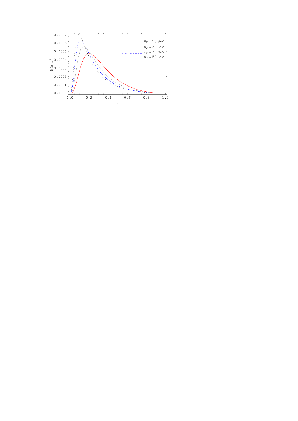
In Fig. 5, the FF of at the starting scale GeV is shown.
The behavior of is shown for different values of the transverse momentum of the gluon.
Note that one of the uncertainties in determination of FFs is due to
the freedom in the choice of scaling variable , i.e. the covariant and non-covariant definitions
presented in Eqs.(3)-(7). As a comparison, our result shown in Fig. 5
is in reliable consistency with the result presented in Fig. 3 of Ref.[10] when the third
definition of fragmentation parameter (Eq. (5)) is applied, i.e. .
Since there are no phenomenological results for the FF, then
at the moment it is not possible for us to compare our result phenomenologically, but
the behavior of our obtained FF in comparison with the and FFs, shown in
Figs. 1 and 2 assures one to rely on our result.
4 Conclusion
The dominant production mechanism for heavy quarkonium at high transverse momentum is fragmentation; the production of a high energy parton followed by its splitting into the heavy quark-antiquark bound states. We showed that the fragmentation function which describes this process can be calculated using perturbative QCD. In this work we gave out the initial fragmentation functions of gluon to split into S-wave charmonium states to leading order in . We used a different approach, Suzuki’s approach, in getting them from the normal analytic calculation in the literatures [10, 12] and found good agreement with the result in [10] when use the normal definition of the fragmentation parameter, i.e. . Finally, although the fragmentation function obtained in this work (3) is schematically for charmonium, in fact it can be directly applied to the S-wave bottomonium sate except that is replaced by and the decay constant is the appropriate constant for the bottomonium mesons.
References
- (1) N. Brambilla, S. Eidelman, B. K. Heltsley, R. Vogt, G. T. Bodwin, E. Eichten, A. D. Frawley and A. B. Meyer et al., Eur. Phys. J. C 71 (2011) 1534 [arXiv:1010.5827 [hep-ph]].
- (2) E. Braaten, M. A. Doncheski, S. Fleming and M. L. Mangano, Phys. Lett. B 333 (1994) 548 [hep-ph/9405407].
- (3) G. T. Bodwin, E. Braaten and G. P. Lepage, Phys. Rev. D 51 (1995) 1125 [Erratum-ibid. D 55 (1997) 5853] [hep-ph/9407339].
- (4) J. C. Collins, Phys. Rev. D 58, 094002 (1998).
- (5) V. N. Gribov and L. N. Lipatov, Sov. J. Nucl. Phys. 15, 438 (1972) [Yad. Fiz. 15, 781 (1972)]; G. Altarelli and G. Parisi, Nucl. Phys. B126, 298 (1977); Yu. L. Dokshitzer, Sov. Phys. JETP 46, 641 (1977) [Zh. Eksp. Teor. Fiz. 73, 1216 (1977)].
- (6) B. Mele, P. Nason, Nucl. Phys. B 361 (1991) 626.
- (7) M. Cacciari and S. Catani, Nucl. Phys. B 617 (2001) 253.
- (8) S. M. M. Nejad and A. Armat, Eur. Phys. J. Plus 128 (2013) 121 [arXiv:1307.6351 [hep-ph]].
- (9) B. A. Kniehl, G. Kramer and S. M. Moosavi Nejad, Nucl. Phys. B 862, 720 (2012); S. M. Moosavi Nejad, Phys. Rev. D 85, 054010 (2012); S. M. Moosavi Nejad, Eur. Phys. J. C 72, 2224 (2012); S. M. M. Moosavi Nejad, Phys. Rev. D 88 (2013) 094011.
- (10) W. Qi, C. F. Qiao and J. X. Wang, Phys. Rev. D 75 (2007) 074012 [hep-ph/0701264].
- (11) J. P. Ma, Nucl. Phys. B 506 (1997) 329.
- (12) E. Braaten and T. C. Yuan, Phys. Rev. Lett. 71 (1993) 1673.
- (13) C. -H. Chang and Y. -Q. Chen, Phys. Lett. B 284 (1992) 127.
- (14) E. Braaten, K. -m. Cheung and T. C. Yuan, Phys. Rev. D 48 (1993) 4230.
- (15) D. M. Scott, Phys. Rev. D 18 (1978) 210.
- (16) M. Hirai and S. Kumano, Prog. Theor. Phys. Suppl. 186, 244 (2010).
- (17) P. Nason and C. Oleari, Nucl. Phys. B 565 (2000) 245.
- (18) M. Cacciari, P. Nason and C. Oleari, JHEP 0604 (2006) 006.
- (19) S. Albino, B. A. Kniehl and G. Kramer, Nucl. Phys. B 725 (2005) 181.
- (20) B. A. Kniehl, G. Kramer and B. Potter, Nucl. Phys. B 582 (2000) 514.
- (21) T. Kneesch, B. A. Kniehl, G. Kramer and I. Schienbein, Nucl. Phys. B 799 (2008) 34.
- (22) P. Nason and B. R. Webber, Nucl. Phys. B 421 (1994) 473 [Erratum-ibid. B 480 (1996) 755].
- (23) M. Soleymaninia, A. N. Khorramian, S. M. Moosavinejad and F. Arbabifar, Phys. Rev. D 88 (2013) 054019.
- (24) C. Peterson, D. Schlatter, I. Schmitt and P. M. Zerwas, Phys. Rev. D 27 (1983) 105.
- (25) B. Andersson, G. Gustafson, G. Ingelman and T. Sjostrand, Phys. Rept. 97 (1983) 31.
- (26) B. R. Webber, Nucl. Phys. B 238 (1984) 492.
- (27) B. A. Kniehl, G. Kramer, I. Schienbein and H. Spiesberger, Phys. Rev. D 84 (2011) 094026.
- (28) A. Heister et al. (ALEPH Collaboration), Phys. Lett. B 512, 30 (2001).
- (29) G. Abbiendi et al. (OPAL Collaboration), Eur. Phys. J. C 29, 463 (2003).
- (30) K. Abe et al. (SLD Collaboration), Phys. Rev. Lett. 84, 4300 (2000); Phys. Rev. D 65, 092006 (2002); 66, 079905(E) (2002).
- (31) M. G. Bowler, Z. Phys. C 11 (1981) 169.
- (32) Belle Collaboration, R. Seuster, et al., Phys. Rev. D 73, 032002 (2006).
- (33) J. D. Bjorken, Phys. Rev. D 17 (1978) 171.
- (34) M. Suzuki, Phys. Lett. B 71 (1977) 139.
- (35) F. Amiri and C. -R. Ji, Phys. Lett. B 195 (1987) 593.
- (36) M. Suzuki, Phys. Rev. D 33 (1986) 676.
- (37) M. A. Gomshi Nobary, J. Phys. G 20, 65 (1994).
- (38) S. J. Brodsky and C. -R. Ji, Phys. Rev. Lett. 55 (1985) 2257.
- (39) F. Amiri, B. C. Harms and C. -R. Ji, Phys. Rev. D 32 (1985) 2982.
- (40) G. T. Bodwin, U-R. Kim and J. Lee, JHEP 1211 (2012) 020 [arXiv:1208.5301 [hep-ph]].