Dynamical Meson Melting in Holography
Abstract
We discuss mesons in thermalizing gluon backgrounds in the
supersymmetric QCD using the gravity dual. We
numerically compute the dynamics of a probe D7-brane in the Vaidya-AdS
geometry that corresponds to a D3-brane background thermalizing from
zero to finite temperatures by energy injection. In static backgrounds,
it has been known that there are two kinds of brane embeddings where
the brane intersects the black hole or not. They correspond to the phases
with melted or stable mesons. In our dynamical setup, we
obtain three cases depending on final temperatures and injection
time scales. The brane stays outside of the black hole horizon when the final
temperature is low, while it intersects the horizon and settles down to the static
equilibrium state when the final temperature is high. Between these two
cases, we find the overeager case where the brane dynamically
intersects the horizon although the final temperature is not high enough
for a static brane to intersect the horizon. The interpretation of this
phenomenon in the dual field theory is meson melting due to
non-thermal effects caused by rapid energy injection.
In addition, we comment on the late time evolution of the brane and a possibility of its reconnection.
AP-GR-108
CCTP-2014-26
CCQCN-2014-17
IPMU14-0004
OCU-PHYS-396
1 Introduction and Summary
1.1 Introduction
The gauge/gravity duality [1, 2, 3] enables us to tackle strongly-coupled gauge theories by using classical gravity. The deconfined phase in the finite-temperature gauge theories is described by the gravity dual in the presence of black holes [4]. This viewpoint has been applied to studying characteristics of the quark-gluon plasma, observed at the RHIC and the LHC experiments. It has been predicted that in the strongly coupled plasma, the shear viscosity over entropy is universally very small [5, 6, 7, 8, 9, 10]. The gravity computations are related with fluid dynamics [11, 12, 13].
An advantage of using the gravity dual is that time-dependent systems can be easily handled. Thermalization and its out-of-equilibrium dynamics are of interest in real-world processes in experiments. In the gravity dual, thermalization is described by black hole formation [14].11 1 A generalization of [14] to inhomogeneous shell collapse is studied in [15, 16]. See also Ref. [17] for a generalization to a confining background. The timescale for the thermalization is typically fast, and the plasma evolution can be understood from hydrodynamic computations [18, 19, 20, 21, 22, 23]. On the other hand, very-far-from-equilibrium effects can be significant in the very beginning of the fast thermalization. We would like to consider such a situation in QCD using the gravity dual.
In this paper, we will study time-dependent dynamics of mesons in fast thermalization in the gauge/gravity duality. In particular, we would like to focus on the initial-stage effects in the thermalization. For that purpose, we will do numerical computations to solve the partial differential equations describing time evolution in the gravity dual. As the setup, we will consider the SQCD realized by D-branes.
The SQCD provides a simple ground for catching qualitative features of QCD-like theories. This theory is realized by D3-branes and D7-branes, where the D7-branes supply fundamental quarks. In the strong coupling in the large- limit, the D3-branes are replaced with the AdS geometry, and we probe the curved background with D7-branes in the limit of [24]. In this paper, we consider the case when .22 2 We may alternatively consider the case that and the D7-branes oscillate coherently. In finite temperatures, the gravity background is the AdS-Schwarzschild black hole with flat horizon [4]. There is no confinement/deconfinement phase transition in the color sector of the SQCD, and the gluons are deconfined in finite temperatures. In the flavor sector, however, if we introduce a nonzero quark mass to explicitly break the global symmetry of the theory, we can find two phases with or without stable mesons, where the parameter is the ratio of the quark mass and the temperature.
The phases are characterized by the embeddings of the D7-branes into the black hole geometry [25]. There are two kinds of embeddings when the system is static. Let us consider units where the quark mass is unity; the parameter is then the temperature determined by the black hole size. In low temperatures, the D7-branes do not touch the black hole horizon, and the fluctuations on the D7-branes give stable mesons [26]. This case is called the Minkowski embedding. In high temperatures, the D7-branes end on the black hole, and the quasi-normal modes on the D7-branes corresponds to melting mesons in the thermal background [27, 28]. This case is called the black hole embedding. The phase transition has been studied in detail in [29, 30, 31, 32, 33, 34].33 3 This phase transition was firstly noticed in the chiral-symmetry breaking D/D system in [35].
Our interest is what happens when we consider dynamical embeddings of the D7-brane in dynamical backgrounds. To address this question, we will compute time evolutions of the D3/D7 system by numerically solving the equations of motion, which are given by partial differential equations.44 4 See Ref. [36] for an earlier study on non-linear dynamics in the D3/D7 system. We consider dynamical embeddings of the probe D7-brane in a D3-brane background corresponding to a system thermalizing from zero to finite temperatures.
1.2 Setup
Let us introduce our setup in a more concrete manner. In this paper, we take the Vaidya-AdS spacetime as the gravity background. In the gravity dual, thermalization is realized by the gravitational collapse and the subsequent black hole formation. The Vaidya-AdS metric is one of the simplest geometry of this kind, obtained for instance as a result of planar-shell collapse [14] or the collapse of null dust.55 5 The Vaidya-AdS metric has been used for studying thermalization in holography, where non-local operators such as the entanglement entropy, spatial geodesic, and Wilson loop are considered [37, 38, 39, 40, 41]. This collapse in the bulk gravity will be identified with a spatially-homogeneous injection of a fixed amount of energy per unit volume in the boundary field theory. We focus on the simplest case of the Vaidya-AdS metric to clarify basic aspects of the dynamical behaviors of the holographic mesons, though in general we could consider more complicated thermalization patterns such as those realized by local heating caused by point particle infalling into the bulk black hole [42] or an anisotropic wake induced by a time-dependent deformation of the boundary metric [43]. The thermalization time scale is typically fast for the Vaidya-AdS metric [44, 45, 46], and hence it would be suitable to focus on the effect of rapid thermalization.
The time evolution we consider is sketched as follows. In the Vaidya-AdS spacetime, it is convenient to use the ingoing Eddington-Finkelstein time as the bulk time coordinate, and coincides with the time of the field theory at the AdS boundary. Initially for , the spacetime is locally pure AdS. We then inject energy from the AdS boundary at to form the black hole that settles down to the Schwarzschild-AdS5 black hole in the final state. The initial static embedding of the D7-brane before the energy injection is given by the analytic solution in the pure AdS spacetime. After the injection, the brane starts to change its embedding shape. We will numerically compute the evolution of the branes. Figure 1 gives schematic illustration when the final mass of the black hole is sufficiently large and the brane intersects with the black hole horizon.

Here, we would like to emphasize subtleties in treating dynamical backgrounds of this kind. When we discuss non-stationary phenomena in the gravity dual description, especially when the event horizon exists, we should pay careful attention to the causality and non-uniqueness of the time foliation of the bulk spacetime, unlikely to static or stationary cases. In our study, such subtleties associated with the bulk causality become manifest when we try to answer questions such as the following:
- •
How should we determine the phase of the brane embeddings at a given time?
- •
How can we know the moment at which the phase transition takes place in the boundary theory?
In static cases, the former question becomes almost trivial: We can distinguish the BH and Minkowski embeddings just by seeing whether the brane intersects with the event horizon or not. In general dynamical cases, however, this naive consideration is no longer suitable. Firstly, there is no definitely preferred time foliation, and this fact implies that the brane configuration at a given bulk time depends on bulk time foliation and is not unique. In addition, the part of the brane world-volume captured in the event horizon cannot be observed by any observers outside the black hole, since that part lies in the causal future of those observers. The information of that part does not affect the dynamics of the other part of the brane outside the black hole, as well as time-dependent boundary observables determined by the brane dynamics.
This observation tells us that some naive notions based on the static cases are no longer rigorous in the dynamical cases. We address this issue in more detail in Sec. 4. In the gauge/gravity duality, it is the dual boundary operators that contains information of the boundary field theory. In our study, we will compute the time evolution of the operators by solving the equation of the motion of the brane. This approach guarantees that the results are not affected by bulk time foliations.
1.3 Summary
Below, we summarize properties of the dynamical D7-brane embeddings clarified by our numerical analysis. Our model possesses two parameters, which are the final black hole mass and the mass injection speed.
We find there are three cases of the dynamical D7-brane embeddings depending on these parameters. Two of them are analogous to static embeddings. If the final black hole mass is sufficiently small, the brane never intersects with the event horizon, and the embedding is the Minkowski embedding with non-decaying oscillations. In the dual field theory, the quark condensate oscillates around the equilibrium value. This is the sub-critical case in which the phase transition does not occur since the final temperature is sufficiently low. If the final mass is sufficiently large, the brane intersects with the horizon, and relaxes to the black hole embedding. This is the super-critical case in which the final temperature is sufficiently high for the phase transition to occur and the mesons are melting.
We find that another kind of dynamical embedding appears when the final black hole mass is slightly smaller than the phase transition value. There is no static BH embeddings in this regime. Despite this fact, the brane dynamically touches the horizon if the injection is sufficiently fast: The rapid injection induces a large brane motion, and it drives the brane into the horizon. Roughly speaking, a part of the brane falls into the black hole because of inertia. We call it the overeager case since the brane is made “overeager” to plunge into the black hole under the influence of the dynamical environment.
After intersecting, the brane configuration on constant surfaces moves in order to escape from the bulk black hole since the final equilibrium configuration in the future cannot be the black hole embedding. The brane configuration, however, tends to be singular within a finite time as the intersection locus approaches the pole where the wrapped by the D7-brane shrinks to zero size. It is expected that if stringy or quantum effects are taken into account there, the brane will reconnect near that locus, and then go back to the Minkowski embedding. We show schematic illustration of this process in Fig. 2(c), together with the sub-critical and super-critical cases in Figs. 2(a) and 2(b), respectively. We argue that this phenomenon may be the gravity dual of quarks recombining into mesons in the boundary field theory.


The remaining of this paper is organized as follows. In Section 2, we will review the static embeddings to fix notations. In Section 3, we describe the setup for our dynamical computation. Results of numerical computations are shown in Section 4. Section 5 is devoted to discussions on the boundary theory interpretations and future directions. Technical details for numerical computations are provided in appendices.
2 Static embeddings
We start from reviewing the static embeddings of the D7-brane to the Schwarzschild-AdS spacetime in order to fix notations. The metric of the Schwarzschild-AdS background can be given as
| (1) |
where , and is the AdS radius. The AdS boundary is at , while the event horizon is at . We use the same world-volume coordinates as the target space coordinates themselves such that , , , . The embedding of the D7-brane is specified by its position in the transverse space as a function of : and . Note that we can set without loss of generality thanks to the -symmetry generated by . The induced metric on the D7-brane is given as
| (2) |
where .
The embedding of the D7-brane is determined by the Dirac–Born–Infeld (DBI) action. In the absence of the world-volume field strength, the action is
| (3) |
where . The equation of motion is a second-order ordinary differential equation for ,
| (4) |
It is also convenient to introduce new bulk coordinates . The new embedding function can then be a function of , . In practical numerical computations, we solve the equation for obtained by rewriting Eq. (4) in terms of .
The asymptotic behavior of the field at the AdS boundary gives information of the dual field theory operators. Near the AdS boundary , the asymptotic solution behaves as66 6 In the notation of Ref. [34], is expanded as . In this notation, the quark mass and condensate are written as and , where is the Hawking temperature and is the ’t Hooft coupling.
| (5) |
where the two integral constants and are related to the quark mass and condensate as [35, 25, 29, 31, 30, 32]
| (6) |
where is the string length and is the string coupling constant. is the quark bilinear associated with its supersymmetric counterparts (See Refs. [34, 47] for further details). Hereafter, we ignore the proportional constants and refer to and as the quark mass and the quark condensate for notational brevity.
In the bulk, we also need to impose boundary conditions at where the D7-brane terminates. The boundary conditions depend on the topology of the embedding, that is, whether the D7-brane intersects the black hole horizon or not. When the brane intersects with the black hole, we impose regularity at the horizon. The asymptotic solution is then obtained as
| (7) |
where () is the value of at the horizon found in the -plane. On the other hand, when the brane does not intersect with the black hole, the brane terminates at the point where wrapped by the brane shrinks to zero size at a pole of : , corresponding to . The regular asymptotic solution at is given by
| (8) |
where is the value of at the pole.
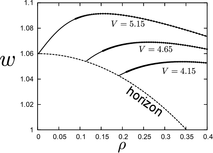
Solving the equations of motion by using either the boundary condition (7) or (8) when the brane intersects with the black hole or not, respectively, we obtain a sequence of embeddings. In Fig. 3, we show the solutions for several parameter values.

For , we can see that both the black hole and Minkowski embeddings are allowed, and they are characterized by different values of the quark condensate for a given . We plot as a function of in Fig. 4.

3 Dynamical embeddings
3.1 Vaidya-AdS5 spacetime
In this section, we consider the very-far-from-equilibrium dynamics of the probe D7-brane in a dynamical spacetime focusing on the thermalization process. Thermalization in the boundary theory is realized in the gravity dual by the black hole formation due to gravitational collapse in the bulk AdS space. In this paper, we use the Vaidya-AdS spacetime as the dynamical background with the black hole formation. Hereafter, we set units where the AdS radius is unity, . The Vaidya-AdS5 metric is given by
| (9) | ||||
| (10) |
where the mass function is a free function representing the Bondi mass (density) of this spacetime. This metric is an exact solution of the following five-dimensional Einstein equation with null dust,
| (11) |
where denotes the ingoing null vector defined by . The null dust injected from the AdS boundary infalls into the bulk, and then the event horizon is formed. When the mass function stops depending on , namely, when the energy injection ceases, the spacetime is locally isometric to the Schwarzschild-AdS5 with a planar horizon.
In our calculations, we chose a function for as
| (12) |
where is the final mass of the spacetime, and determines the duration of the energy injection. Note that the final radius of the event horizon, , is given by . Uplifting the solution to -dimensions, we obtain Vaidya-AdS spacetime:
| (13) |
We consider the probe branes on this -dimensional background geometry. Figure 1 gives schematic illustration of our setting, as explained in Sec. 1.2.
3.2 Evolution equations of the D7-brane
Having explained the background spacetime, we proceed to consider evolution equations of the D-brane to solve dynamical embeddings numerically. Dynamics of a probe D-brane is described by the DBI action. It has the diffeomorphism invariance with respect to transformations of world-volume coordinates. We should choose some useful coordinates, namely fix the gauge, for solving the evolution equations numerically. In order to derive equations of motion taking advantage of coordinate transformations on the brane, here we would like to begin with the Polyakov type action instead of the DBI action. Of course, once we know the appropriate ansatz, we could simply start from the DBI action to derive the equations of motion. The result is the same as that obtained from the Polyakov type action since the computation is on-shell.
The Polyakov type action for the D7-brane in the absence of the world-volume field strength is given by
| (14) |
where is the brane collective coordinate and is the metric in the target space. Note that is an arbitrary non-zero constant. Variating the action with respect to and , we obtain the equations of motion of the D7-brane as77 7 Using Eq. (16) and eliminating the auxiliary field from the action (14), we obtain Dirac–Nambu–Goto action: .
| (15) | ||||
| (16) |
where is the covariant derivative with respect to , and is the Christoffel symbol with respect to . The second equation implies that can be regarded as the induced metric on the brane up to a factor . One finds that the wave equations (15) for on the world-volume with the induced metric are evolution equations, and the equations (16) which determine components of the induced metric are constraint equations. In the following, we will study the D7-brane embeddings on the Vaidya-AdS background spacetimes solving Eqs. (15) and (16).
There are eight world-volume coordinates () on the brane. For six of them, we use the target space coordinates themselves as because we assume that the brane has the same symmetry as the background bulk spacetime in those directions. For the other two coordinates, we introduce the double null coordinates , and then the brane collective coordinates are parametrized as
| (17) |
where we set without loss of generality because of the -symmetry generated by . The -coordinates are chosen so that the and are null generators. Then, the brane induced metric is written as
| (18) |
In the following calculation, it is convenient to use a new variable instead of . From the -component of Eq. (16), we can express in term of as
| (19) |
Note that there are still residual coordinate freedoms on the world-volume,
| (20) |
This residual gauge freedom will be fixed by boundary conditions and an initial condition. Substituting Eqs. (17) and (18) into Eq. (15), we can obtain evolution equations for , and .
The equations we will solve are summarized as follows. The evolution equations for , and are obtained as
| (21) | ||||
| (22) | ||||
| (23) |
From the requirements that the and -components of Eq. (16) vanish, we obtain the constraint equations,
| (24) | ||||
| (25) |
Note that the evolution equations guarantee the conservation of the constraints:
| (26) |
Consequently, once we set an initial data satisfying the constraint equations, we may solve only the evolution equations as the constraints will be kept satisfied. The details of the numerical method to solve these equations are summarized in Appendix A.
Eliminating and , we can regard as a function of and . Near the AdS boundary , is expanded as
| (27) |
The constant and the function are related to the quark mass and condensate as in Eqs. (6). Solving the evolution equations, we can determine the time dependence of the quark condensate .
3.3 Boundary conditions and initial data
In general, two timelike boundaries appear on the world-volume of the brane: one is the AdS boundary , and the other is the pole at which the radius of wrapped by the D7-brane shrinks to zero. When a numerical domain to be solved contains these boundaries, we need to impose boundary conditions there. Since, however, the evolution equations become singular at each boundary, we should fix the location of the boundary in the world-volume -coordinates for numerical convenience.
As mentioned previously, we have the residual gauge freedom, which is a transformation from the original null coordinates to other ones (20). This is nothing but a conformal transformation between two-dimensional flat spacetimes. Using it, one can fix the location of the AdS boundary on the world-volume coordinates as , i.e. , or that of the pole as , i.e. , or both. They become coordinate conditions on the world-volume domain.
Note that fixing the residual gauge is equivalent to choosing a certain conformal factor, which behaves as a harmonic function obeying a -dimensional free massless field equation.88 8 We denote a conformal transformation as . In two dimensions, the scalar curvature is , where is the covariant derivative with respect to . Now, since both and are flat, namely and , the conformal factor must be determined by a harmonic function satisfying . Hence, if we give a set of coordinate conditions at the boundaries and the initial surface, they will provide necessary boundary and initial conditions for the conformal factor. Those conditions will fix the residual gauge completely, and the null-coordinate system will be automatically determined on the computational domain.
3.3.1 Boundary conditions at the AdS boundary
Now, we derive boundary conditions at the AdS boundary. Since we will focus on observables there, the AdS boundary should be always contained in our computational domain and located at throughout our calculations. The boundary conditions for and are trivial: and . We choose the quark mass as time-independent, namely is constant. Remaining boundary conditions on the AdS boundary can be derived by requiring regularities of the evolution equations at . We expand the variables near the boundary as , and . Substituting them into the evolution equations (21)–(23), we obtain the asymptotic solution as
| (28) |
where . They give
| (29) |
Hence, integrating along the AdS boundary, we can determine the time evolution of . (The second equation is used to determine at the boundary. For details, see appendix A.) Note that while the regularities yield or , we have taken because the time direction in our setup leads to . We can confirm that and (it is equivalent to the first equation of (29)) are consistent with the constraint equations at the AdS boundary.
3.3.2 Boundary conditions at the pole
Next, we consider the boundary conditions at the pole, at which the radius of wrapped by the D7-brane shrinks to zero. The brane may intersect with the event horizon in our calculations, and in that case we do not need to impose the boundary conditions at the pole since the AdS boundary is not in the causal future of the pole on the brane. Strictly speaking, when our computational domain does not contain this boundary, we do not need any boundary conditions there. If we need the boundary conditions, we will locate the pole at by using the residual gauge. Hence, one of the boundary conditions is . The others are given by regularities of the evolution equations at as
| (30) |
at . They are merely Neumann boundary conditions at the pole.
3.3.3 Initial data
Finally, we explain the initial data for our calculations. Before the energy injection , the background spacetime is pure AdS, and the brane is static there. We have the exact solution of the static embedding given by , i.e., . Solving the constraint equations (24) and (25), we obtain
| (31) |
where is a free function corresponding to the residual coordinate freedom, and is an integration constant. At the initial surface , the solutions become
| (32) |
where we have set , and then is the initial time at the AdS boundary.
The residual gauge corresponds to the coordinate freedom for on the initial surface, and then we can choose an appropriate function for arbitrarily. When the brane does not intersect with the event horizon, we can simply choose . In this case, the pole can be fixed at .
If the brane intersects with the event horizon at the initial surface, or if the brane is close to the event horizon, the above choice is not good. The reason is as follows. Each -constant line represents an out-going null geodesic on the brane world-volume. Roughly speaking, is a proper distance between two null geodesics described by and at the initial surface. If these out-going null geodesics pass through the vicinity of the event horizon towards the AdS boundary, the interval of each arrival time at the AdS boundary, , will become very large compared to the proper distance at the initial surface.99 9 Rough estimation is , where is a surface gravity and is the coordinate value describing the event horizon. This behavior essentially originates from the gravitational red-shift effect near the horizon. As a result, if we choose , blows up rapidly at late time and then the numerical calculations easily break down.
To avoid this problem, we fine-tune so that and are synchronized at the AdS boundary, i.e., (or ). This implies that becomes exponentially small in the vicinity of the event horizon. In Appendix A, we explain how to fine-tune in our numerical calculations.
Note that the condition is another boundary condition at the AdS boundary imposed in addition to the one that fixes the boundary position at . This means that we do not fix the location of the pole on the world-volume coordinates. However, this is not a problem because the pole is not contained in our computational domain and then we do not need to impose the boundary conditions there.
4 Results
In this section, we show results of our numerical calculations. We use units in which .1010 10 In our system, there is a scaling symmetry: , , , , , , , and , where is a constant. Using the scaling symmetry, we can set without loss of generality. The parameters are the final mass of the black hole (in other words, the final temperature) and the duration of the energy injection, which are respectively described by and .
4.1 Sub-critical case
In this subsection, we show numerical results for the small final mass case in which the D-brane does not touch the horizon and remains in the Minkowski embedding after the black hole formation. This is the sub-critical case in which the final temperature is sufficiently low and the phase transition does not occur. Since there is no dissipation when the brane is in the Minkowski embedding, excitations on the brane caused by dynamics of the bulk geometry will remain without decay.
Figure 5 shows the time evolution of the quark condensate and the Bondi mass with respect to the boundary time . Note that all of these quantities are well-defined at the AdS boundary and are directly related with observables in the boundary theory. The Bondi mass corresponds to the energy density of the CFT (gluon) fluid. We can recognize seemingly periodic oscillations after the energy injection. These correspond to excitations of stable mesons, namely normal modes of the brane fluctuations. Indeed, the power spectrum of shown in Fig. 6 obviously indicates that the excitations have discrete spectrum, similarly to the case of linear perturbations on the static Minkowski embedding. Note that we have solved non-linear evolution equations of the brane rather than linear perturbations around an equilibrium brane configuration, and the discrete spectrum is a nonlinear version of the normal mode spectrum for linear fluctuations.


Figure 7(a) shows time evolutions of for various . It turns out that the shorter the injection duration is, the harder the condensate oscillates. This implies that the larger non-adiabaticity is, the larger the excitations on the brane are. To study the fluctuations in more detail, we show the total power of fluctuations of the condensate, , in Fig. 7(b). We calculated for setting the final horizon radius to , and obtained from using and . We confirmed that the numerical results are almost independent of as long as we keep it larger than . The numerical results imply that shows a damped oscillation whose amplitude behaves as , and appears to converge into the finite maximum value in the limit.
Before moving to the next subsection, we make some comments on the relationship of these results to a harmonic oscillator model. We find that features of can be well reproduced by a harmonic oscillator with an external force described by , if we take of Eq. (12) as the external force . The total oscillation power in the final state of this model is given by , where is a normalization constant independent of .1111 11 When is set to of Eq. (12) and the initial state is set to , we can show that the total power at late time () is given by , where is the equilibrium point of the oscillator at late time and is the average of a function over a time period sufficiently longer than . When is changed into that of Eq. (33), the total power at late time changes into . Fitting this analytic formula to the numerical data, we obtain . This value coincides with the lowest normal mode frequency of the brane oscillations (see Fig. 6).


Precise behavior of depends on the function form of . As an example, in Fig. 8 we show for given by
| (33) |
For this , shows a damped oscillation that decays as . Similarly to the previous case, this numerical result is well reproduced by a harmonic oscillator model: When is set to of Eq. (33), the model gives , where the constant is independent of . Fitting to the numerical data gives , and this value coincides with the lowest normal mode frequency.
These results suggest that some aspects of the time dependence of the D7-brane and the condensate can be captured by the harmonic oscillator model with the external force . For example, the right-hand sides of the equations of motion (21)–(23) contain terms proportional to , and those terms may be roughly identified with the external force applied to the D7-brane. It may be interesting to pursue these ideas in more detail. Also, it may be interesting to study further on behaviors in the limit to give an estimate on the largest amplitude realized by a rapid energy injection. Our numerical results and the analytic results based on the harmonic oscillator model in this context suggest that converges to finite constants in the limit. It may be interesting to generalize results of Ref. [48], which focuses on abrupt quenches in the holographic setup, to the D3/D7 system and compare them with our results.

4.2 Super-critical case
In this subsection, we show numerical results for the large final mass case in which the D7-brane is drawn into the event horizon and its configuration changes from the Minkowski embedding to the BH embedding. This is the super-critical case in which the final temperature is sufficiently high for the phase transition to occur.
In Fig. 9, we show a typical behavior of the quark condensate and the black hole mass in this case, setting the energy injection duration to . The quark condensate gradually evolves as the black hole mass increases due to the injection, and eventually settles down to the final value by . This final value coincides with of the static BH embedding for the same bulk black hole mass. It turns out that a quasi-normal mode is excited in the ring-down phase. This fact implies that the phase transition to the BH phase has taken place and the brane comes to equilibrium.

In Fig. 10, to focus on the brane world-volume in the bulk, we show snapshots of the brane configuration on time slices characterized by . Note that we define the bulk coordinates on the time slices as . The radius of the event horizon is evolving larger, and we can see that the brane eventually intersects with the horizon. At late time the configuration of the brane will coincide with the static BH embedding.

When we consider dynamical phenomena in the bulk, especially when an event horizon exists, we should pay careful attention to the causality. In the static case, two meson phases of the boundary field theory can be distinguished by seeing whether the brane configuration at any moment is intersecting with the horizon or not. However, such a naive definition can not be used in dynamical cases by the following reason. A temporal configuration of the brane, which is the intersection of the brane world-volume and a certain time slice of the bulk, depends on the given time slice. Since there is no definitely preferred time slice in general spacetime, we cannot uniquely identify the phase of the brane embedding according to the temporal configuration at that time. To see it, let us consider the following example for time slices determined by In the current case, the event horizon does exist even before the injection starts and when the bulk spacetime is still locally pure AdS. The brane can enter the horizon within this early time domain. It means that the brane can intersect with the event horizon even at (before the injection starts!). However, the brane configuration in that time domain is given by the exact solution in the pure AdS, and it will be obviously regarded as the Minkowski embedding if static.
In the spirit of the gauge/gravity duality, to determine the phase of the brane embedding, we should look at the quark condensate rather than the temporal configuration of the brane on a certain time slice. If we consider the causality in the bulk further, we notice that observers outside the black hole (including those on the AdS boundary) cannot know whether the brane intersects the horizon or not, since the intersection locus lies on the event horizon and the exterior observers can never obtain information on that locus. This implies that an attempt to determine the phase based on the temporal brane configuration requires information inaccessible from the boundary. On the other hand, the behavior of the quark condensate is defined only by the information outside the horizon, since this quantity is governed by the brane equations of motion that respect the bulk causality. Indeed, using the quark condensate , we can examine the phase of the brane embedding without any problem, as shown in Fig 9. From the viewpoint of the boundary, the phase transition takes place when the brane is drawn into the vicinity of the black hole (namely, when the gravitational red-shift at the brane becomes strong) rather than the inside of that.
4.3 Overeager case
As a new significant feature in the dynamical evolution, we find that the brane can fall into the event horizon even in a parameter region where any equilibrium BH embedding does not exist. We would like to refer to this situation as the overeager case, as explained in Sec. 1.3. Figure 11 shows the time evolution of quark condensate and the black hole mass in such an overeager case. The time evolution of markedly differs from the previous cases: There are neither periodic oscillations nor relaxation to the equilibrium value. Also, we show snapshots of the brane configuration at early time () and late time () in Figs. 12 and 13, respectively. We take as the final radius of the black hole, for which only the Minkowski embedding exists as the static brane configuration (see Fig. 4). However, the brane configurations in Figs. 12 and 13 indicate that the brane intersects with the event horizon. This fact is reflected in the non-periodic behavior of . We also notice that the brane keeps moving even after the bulk spacetime has settled down to the final state.


We can understand this bulk phenomenon in the following way. It is not forbidden that a part of the brane dynamically intersects with the event horizon even if any static BH embedding does not exist.1212 12 In a special case, this statement can be easily proved as follows. When is infinitesimal, namely for the fastest injection, the radius of the event horizon becomes just at and it will be the final radius. On the other hand, if the quark mass is , the tip of the static brane is located at before the injection . This implies that the portion of the brane near the tip resides within the event horizon at . Since there is no equilibrium BH embedding for , the brane must be overeager in such cases. Once some part of the brane oversteps the horizon, that part can never come out from the horizon by the definition of the event horizon. Since no equilibrium configuration as the BH embedding exists, the brane has no choice but to remain dynamical with intersecting the horizon.
It is worth noting that it depends on the energy injection duration whether this overeager case is realized or not. As we mentioned in Sec. 4.1, the excitations on the brane become larger as the energy injection becomes faster. Therefore, it is expected that if the energy injection is sufficiently slow, the brane can not be overeager. In fact, we can see this expectation is true. Figure 14 shows time evolution of in a case of slow injection. This reveals that the quark condensate is periodically oscillating around the equilibrium value, and its behavior is different from the one in the overeager case shown previously. This result implies that the brane is the Minkowski embedding with periodic oscillations in the sub-critical cases. Thus, non-adiabaticity of the energy injection plays an important role in the overeager effect.

Are the mesons melting in the overeager case? As shown in Fig. 11, the quark condensate shows a damped oscillation around the smooth time-evolving component, while the normal-mode oscillations present in the sub-critical case is absent in this case. Also, if we focus on the snapshots of the brane configuration on constant surfaces, we find that the brane touches the bulk black hole for a time scale relatively longer than that of the thermalization (see Fig. 13). These facts suggest that the meson is melting in the overeager case, though the temperature of the bulk black hole is lower than the critical one. We argue the dual field theory implications of this overeager case in Sec. 5.1.
4.4 Final fate for the overeager case
What will be the final brane configuration of the time evolution in the overeager case? As mentioned in the previous subsection, there is no corresponding static BH embedding. As explained in Appendix A, we can solve the evolution equations only outside of the event horizon and the red-shift prevents us from computing in the region very close to the horizon. For these reasons, we do not have whole numerical solutions of the brane configuration at late time. In this subsection, to infer a final fate of the overeager case, we extrapolate numerical solutions of the brane configuration using the Padé approximation, and estimate late-time evolutions of the brane.
Let us define where is the minimum value of in our numerical data at each bulk time. This parameter measures the distance of the extrapolation. We use numerical data satisfying in this subsection. Figure 15(a) shows the brane configuration for several late-time -constant slices: . We set parameters as and . Our numerical data are plotted by black dots and their inter/extrapolation are depicted by solid curves. We see that, at , the brane position on the horizon reaches the pole, at which the radius of the wrapped by the brane becomes zero. In Fig. 15(b), we plot the radius of the on the horizon, , as a function of . In this figure, numerical data with and are shown by black and white circles, respectively. From the figure, we can see that the radius of becomes small as time increases, and it seems to reach zero within finite time. Since the extrapolation of the brane shape employed here may cease to be a good approximation near the horizon and the pole when becomes large, the precise motion of the brane at late time could be different from that described here in that case. However, these results with a help of the extrapolation imply that the brane would reach the pole in the neighborhood outside the horizon around and the brane embedding would be singular.1313 13 Originally, the tip of the brane is located at the pole and the embedding is regular there. If the embedding is regular at , the tip of the brane must be just at the pole on the horizon. However, the tip of the brane has fallen into the black hole and a regular tip cannot be at the pole on the horizon. This implies that other parts of the brane have concentrated on the pole and the embedding would be singular. Classical description of the brane would break down at such a singular point and a singularity outside the horizon could be seen from the boundary.

If we take into account stringy effects, there is a possibility that the brane reconnects near the pole around . When the radius of the wrapped by the brane becomes small, we may expect that brane will reconnect. Let us estimate the condition for the brane reconnection. The radius of the is given by where we defined . Note that we have restored the AdS curvature scale , which is the radius of too. The condition for the reconnection is given by , and it can be rewritten as , where is the ’t Hooft coupling defined by . This inequality indicates that, if we take into account the stringy (finite ) effect, emergence of the singularity may be avoided by the brane reconnection. In a similar manner, the reconnection may occur by taking bulk quantum effects into account via membrane nucleation. Once the reconnection occurs, the part of the brane connected to the boundary would be separated from the black hole and oscillate around the equilibrium configuration, which is the static Minkowski embedding determined by the bulk black hole mass.
5 Discussions
5.1 Boundary theory interpretations
We discuss boundary theory interpretations and implications of our numerical results, especially focusing on the overeager case. In this case, the brane touches the horizon temporarily and tends to be singular in a finite time duration. If we take into account stringy or quantum effects in account, the brane may reconnect near the singular point, and go back to the Minkowski embedding with oscillations induced by the reconnection. We consider this process in the boundary theory point of view below.
In the overeager case, the meson is melting even though the final temperature of the gluon medium (represented by the thermal D3 background) is lower than the meson melting temperature. One possible explanation for this phenomenon would be as follows. A rapid energy injection drives the ambient gluon medium into a non-thermal state. In such a state, the distribution function of the gluons will be deformed from the thermal one governed by its temperature. If the deformed distribution function possesses sufficient amount of high-energy components, gluons would break bound states of quarks and melt the mesons. It would be interesting if we could examine such a scenario from the bulk point of view. For example, the spectrum of the bulk Hawking radiation corresponds to the distribution function of the gluon medium mentioned above, and can be studied using techniques of Refs. [49, 50]. Such a study would provide useful information for this issue.
At the late time of the overeager case, the gluon medium approaches thermal equilibrium and high-energy gluons decrease. Since the final temperature is lower than the meson melting temperature, some of the dissociated quarks and antiquarks will recombine into mesons giving off the latent heat into the mesons and the gluon medium. The recombination of mesons may correspond to the reconnection of the D7-brane in the gravity side.
5.2 Open questions and Future directions
We have clarified some basic aspects of dynamics in the D3/D7 system with the aid of numerics in this paper, but we still have many open questions to be addressed. Below, we list them along with ideas for future directions of the study.
- •
Applications to other systems:
In this paper, we have developed a numerical scheme that realizes a robust time evolution for a long duration to study the probe brane on the dynamical background spacetime. This technique and its generalizations may have various applications to study non-linear dynamics within the context of the gauge/gravity duality.
One possibility is to apply to more general brane systems. An example is the black hole-string system like those studied in Ref. [51], which corresponds to the quarks moving in the thermal plasma medium. Our scheme will enable to consider the effect of the dynamical background and relaxation phenomena therein. It will be interesting also to consider brane systems that realize more realistic field theories, in particular those realizing confinement, such as the D4/D6 system [35] or the Sakai-Sugimoto model [52]. We did not include the world-volume field strength and external fields in this paper, and their effects deserve further investigation (see e.g. Ref. [36] for the effect of external magnetic field).
Yet another future direction is to consider higher-cohomogeneity cases. For example, Ref. [42] considered a similar melting process realized by a rapidly-moving point particle modeled by the Aichelberg-Sexl solution in the bulk. Starting from a system whose temperature is slightly below the melting temperature and using the near-horizon approximation, they shown that the mesons melt in a spatially localized region whose size is larger than the scale naturally expected from the injected energy and the temperature difference from the melting temperature by a factor of . This behavior is qualitatively similar to that of the overeager case, in the sense that the it becomes easier to melt mesons in the non-equilibrium regime. They focused on the regime where , and then it will be interesting to see how this behavior changes in general cases. Also, it may deserve to study if the phase corresponding to the overeager case, in which the mesons melt at temperature lower than the critical one, persists in this local heating case.
- •
Brane motion and reconnection:
We observed that, in the overeager case, the intersection locus of the brane and bulk horizon moves toward the pole, where a brane reconnection is expected to occur. It would be interesting to clarify the brane dynamics after the reconnection assuming an explicit reconnection process or taking into account effects beyond the DBI action. Dynamical processes involving a brane and a black hole have been studied in, e.g., Refs. [53, 54, 55, 56] in the context of braneworld models, and these previous results may give us implications to the physics after the brane reconnection or the quark recombination. Also, it would be important to understand influence of the effects beyond the DBI action, such as the curvature corrections arising from non-zero brane thickness [57, 58, 59, 60, 61].
One possible way to analyze the brane dynamics in a simplified manner is to focus on the near-horizon region. Ref. [62] studied static brane configurations in the near-horizon region. They constructed a family of static solutions in that region and clarified its basic properties. Also Ref. [42] focused on the near-horizon region in the D3/D7 system, and clarified the brane motion just after the local heating as explained above. It may be interesting to study the brane dynamics in this setup, especially focusing on the regime where the reconnection occurs.
- •
Brane induced geometry and fluctuations:
We may read out some extra pieces of information from the induced geometry on the D7-brane. Fluctuations of the brane is governed by the induced geometry, since the intrinsic curvature gives rise an effective potential for those fluctuations. By studying the relationship between the intrinsic geometry and the (quasi-)normal mode frequency of the brane fluctuations, we may achieve a better understanding on the time dependence of from the bulk point of view.
In this context, it is interesting to focus on the overeager case, where the brane turns from the BH embedding into the Minkowski embedding at some moment. A naive expectation is that the decay rate of the quasi-normal modes becomes smaller as the transition time approaches, since it becomes zero after the transition. The intrinsic curvature tends to singular in this process, and it may cause such a time dependence through the effective potential for the fluctuations. It will be interesting to test this conjecture by comparing the time dependence of the brane intrinsic curvature and the brane fluctuations. Also, this transition can be viewed as a black hole formation and subsequent evaporation in the brane induced geometry. It may deserve a further consideration if we can relate such an idea with the time dependence of the brane fluctuations and .
In Fig. 6, we observed that the discrete spectrum of in the Minkowski embedding shows a exponential decay at higher frequency region. We may be able to read out a characteristic scale from this exponential decay. It might be interesting to elaborate this idea further, though this kind of exponential decay in the spectrum could be simply due to basic properties of the decomposition of the initial perturbations into the normal modes at high frequency band (see e.g. Ref. [63] for behavior of Fourier coefficients in the high-frequency limit).
Acknowledgments
We thank Norichika Sago and Takashi Hiramatsu for helpful advice about numerical calculations. We also would like to thank Don Marolf, Helvi Witek and Takahiro Tanaka for valuable comments. The work of TI is supported in part by European Union’s Seventh Framework Programme under grant agreements ((FP7-REGPOT-2012-2013-1) no 316165, PIF-GA-2011-300984, the EU program “Thales” and “HERAKLEITOS II” ESF/NSRF 2007-2013 and is also co-financed by the European Union (European Social Fund, ESF) and Greek national funds through the Operational Program “Education and Lifelong Learning” of the National Strategic Reference Framework (NSRF) under “Funding of proposals that have received a positive evaluation in the 3rd and 4th Call of ERC Grant Schemes”. SK is partially supported by the JSPS Strategic Young Researcher Overseas Visits Program for Accelerating Brain Circulation “Deeping and Evolution of Mathematics and Physics, Building of International Network Hub based on OCAMI”. The work of NT is supported in part by World Premier International Research Center Initiative (WPI Initiative), MEXT, Japan, and JSPS Grant-in-Aid for Scientific Research 25755.
Appendix A Numerical methods
In this appendix, we explain our numerical methods to solve the time evolution of the D7-brane. We need two kinds of numerical schemes depending on whether the brane intersects with the event horizon or not. Before and after the brane intersects with the event horizon, we use numerical method in subsection A.1 and A.2, respectively.
A.1 Before the brane intersects with the event horizon
In this section, we explain our numerical method before the brane intersects with the event horizon.1414 14 If the brane intersects with the event horizon at the initial surface, which occurs when the initial background temperature is sufficiently large, we use the method in section A.2 from the beginning.
A.1.1 Evolution scheme
The time evolution of the D7-brane is described by non-linear wave equations (21)–(23). We will use the finite-difference method for solving them numerically. It turns out that the time evolution based on these equations is numerically unstable. To stabilize it, we eliminate and in the right hand side of the equations using the constraints (24) and (25) as
| (34) |
where each sign in the front of the square root is determined by the boundary conditions at , namely and , or and . As a result, the evolution equations can be schematically rewritten as
| (35) |
where and . We can realize a stable numerical time evolution if we use these equations as the evolution equations.1515 15 We found the method to stabilize the numerical calculation by trial and error, and the reason of the stabilization is unclear at this moment. It will be useful to clarify the stabilization mechanism, especially when we try to apply this numerical method to more generalized systems. One way to analyze it would be to show the well-posedness of the evolution equations, employing arguments similar to those in Ref. [64, 65, 66, 67]. As shown in Fig. 16, we discretize and coordinates with the grid spacing . Now, we focus on the points N, E, W, S and C in the figure. We can evaluate the function and its derivatives at point C with second-order accuracy as
| (36) |
where the index of denotes each point N, E, W or S at which is evaluated. Substituting the above expressions into Eq. (35), we obtain nonlinear equations for . Solving the nonlinear equations by the Newton-Raphson method or the predictor-corrector method, we can determine unknown value of from , and which have been already given.

A.1.2 Boundary conditions at the AdS boundary
One of the boundaries in our numerical domain is the AdS boundary, . As we explained in section 3.3, we fix the location of the AdS boundary at by using a residual coordinate freedom throughout our calculations. Suppose that the point C is located on . The boundary conditions for and leads to and (where the quark mass is unity), shortly. For , the boundary conditions (29) are discretized as
| (37) |
where the point E is a dummy grid point introduced in order to impose the boundary conditions. From on the boundary, we obtain
| (38) |
This equation determines the time evolution of at the AdS boundary.
A.1.3 Boundary conditions at the pole
The other boundary is the pole, , at which the radius of wrapped by the D7-brane shrinks to zero. We set the location of the pole at . For and , we have the Neumann boundary conditions as
| (39) |
at . (If we introduce Cartesian coordinates and , they are rewritten as .) Now, we focus on the points P, Q and R in Fig. 16. Since and satisfy the Neumann boundary conditions, we can approximate them by quadratic functions as and near the pole. We can determine , , and from values of and at the points Q and R. As a result, we obtain
| (40) |
These expressions are essentially the backward differences of and at the point P of second-order accuracy in the spatial direction. For , we have as the boundary condition. Note that we need to know the values of , and at the points Q and R prior to imposing these boundary conditions the point P. It is possible if we solve the evolution equations initially along -direction and then proceed to the next step along -direction.
A.1.4 Initial data and time evolution
We impose initial data as Eq. (32) on the initial surface . Since we have located the AdS boundary and the pole at and , respectively, the function , which is the residual coordinate freedom, should be . For simplicity, we will choose here. Now, we can solve the time evolution in the current numerical scheme until the brane intersects with the event horizon. However, if the brane has intersected with the event horizon, will blow up rapidly near the horizon along -direction and our numerical calculation will be broken immediately after the intersection. Therefore, we should monitor values of and at the pole for each -slice. If the pole is inside the horizon, , we pause the numerical integration at a intermediate surface and switch to the other scheme explained in the following subsection. Then, we will restart to integrate taking the numerical solution on the intermediate surface as the initial data for the new scheme. We denote the solutions on the intermediate surface as , and . On the intermediate surface, the -coordinate is defined in . The lower and upper bounds of the inequality correspond to the AdS boundary and the pole, respectively. Since the solutions on the intermediate surface are obtained just on grid points, we interpolate them by polynomials and regard them as functions in to construct the initial data for the new scheme.
A.2 Time evolution after the brane intersects with the event horizon
Here, we explain the numerical method after the brane intersects with the event horizon. The evolution scheme and the boundary conditions at the AdS boundary are the same as shown in Sec. A.1.1 and Sec. A.1.2. At the pole, we do not need to impose any boundary conditions because it is already inside the event horizon and is no longer contained in the current numerical domain.
As the initial data, we use the functions , and , obtained in the last subsection. If the brane has intersected with the event horizon at an initial surface or if the brane will intersect shortly after the energy injection, we use Eq. (32) as the initial data from the beginning. As we mentioned before, at the AdS boundary blows up if the brane is close to the event horizon. To avoid it, we will adopt a coordinate system to synchronize, at the AdS boundary, the coordinate time on the world-volume with the asymptotic time using the residual coordinate freedom at the initial surface. We consider the coordinate transformation on the initial surface as . Then, the -coordinate is also transformed as to locate the AdS boundary at . We choose this free function so that and are synchronized up to a constant at the AdS boundary, i.e., .
Hereafter, we explain how to determine the which synchronizes and . As in Fig. 17, we take the domain of -coordinate as and discretize it as (). We denote and set . We also denote boundary values of at each grid point as , , , . We determine the numerical solution in the order of . (Roughly speaking, we regard as the “time” coordinate.) Firstly, we solve the evolution equations at using a trial value .1616 16 In our calculation, we used and for . Then, at the point , we obtain an asymptotic time at the AdS boundary. Since we would like to synchronize and at the AdS boundary (namely, ), the appropriate choice of should be
| (41) |
For this choice of , we recalculate the evolutions and obtain . Next, we solve the evolution equations at and with a trial value and obtain an asymptotic time at the AdS boundary. Since we would like to impose , we should choose as
| (42) |
Then, we recalculate them and obtain . By repeating this procedure, we can synchronize and at the AdS boundary. Note that, in this choice of free function , our numerical domain does not touch the event horizon since, along a -constant surface, the function approaches a finite value at the AdS boundary and the surface should be outside the horizon. (Intuitively speaking, observers at the AdS boundary cannot see the event horizon within finite asymptotic time.) In principle, we can solve the time evolution forever () by the current scheme in contrast to the previous scheme in Sec. A.1. However, especially in the overeager case, numerical error accumulate in actual calculations and it becomes an obstacle for an numerical evolution over a long time duration. In a typical set up, our numerical calculation is reliable in at least, which is sufficient for our purpose.

Appendix B Error analysis
We test our numerical code by (i) checking if a static initial data remains static in the time evolution by our code, and (ii) showing second-order convergence of the constraints. Our code passes these tests as shown below.
B.1 Static initial data
B.1.1 Vacuum bulk
When the bulk spacetime is the pure AdS spacetime without a black hole, the static initial data is exactly given by Eq. (32). We check if our time evolution code keeps it to be static and the quark-condensate to be zero.


We show in this case in Fig. 18(a) for grid number . For each , is approximately given by an constant component with periodic pulse noise, whose detailed structure is shown in Fig. 18(b). These sharp peaks are generated by time evolution near the pole, where the evolution equations become singular.
We show the dependence of the constant component and the peak height around it in Fig. 18(c), where we defined the average value of , , by numerically fitting to a constant over , and the peak height by . Fitting the numerical data, we find that both the constant component and the peak height around it converge to zero as we increase by power-law with powers and , respectively.
B.1.2 Bulk with a black hole
We also test if static initial data remains static in the time evolution given by our code even when a bulk black hole exists. For this purpose, we construct static initial data by integrating Eq. (4) numerically, and studied time dependence of provided by that.


We show for the static Minkowski embedding by Eq. (4) for the black hole mass (the horizon radius ) in Fig. 19(a). Similarly to the previous case, is approximately composed of constant component and periodic pulse noise around it (see Fig. 19(b)). We calculate the average value of the quark condensate by fitting to a constant over for each . This average value depends on , and its asymptotic value, , is estimated by fitting numerically. We show the result of the fitting in Fig. 19(c), from which we see that converges into by power law with . The peak height around the average is obtained by for each , and it converges to zero by power law with at least up to .


Next, we show for the static black hole embedding for in Fig. 20(a). For each , converges to its final value after some oscillations around it. Fitting shows that the average for converges to an asymptotic value by power law with . Also, the maximum deviation of from the average converges to zero by power law with .
B.2 Constraint violation
In this section, we check that the constraint violation is maintained to be sufficiently small in the dynamical calculations shown in Sec. 4. We show that the constraint violation is sufficiently small throughout the time domain discussed therein, and also that it shows second-order convergence when the resolution is raised.
B.2.1 Dynamical Minkowski embedding
Taking the numerical calculation for the results shown in Fig. 14 with and as an example, we study the resolution dependence of the constraint violation. For this purpose, we define rescaled constraints by
| (43) | ||||
| (44) |
by removing the overall factor from Eqs. (24) and (25) and taking their absolute values.


We show at in Fig. 21(a). We find that for any at . To study the time dependence more precisely, we show at for in Fig. 21(b) for . This plot suggests that the average of roughly stays constant for . shares a similar property. In Fig. 21(c), we show the average obtained by fitting for to constants for various . Numerically fitting , we find they converge to zero by power law with and , respectively.
B.2.2 Dynamical black hole embedding
Below, we show the constraint violation for the dynamical black hole embeddings discussed in Secs. 4.2 and 4.3.
Figure 22 shows the constraint violation for the super-critical case with and dealt in Sec. 4.2. at and that at are plotted in Figs. 22(a) and 22(b), respectively. Plots for become qualitatively similar to them. The average value of at over , , converges to zero by power law with and , respectively.


Figure 23 shows the constraint violation for the overeager case with and dealt in Sec. 4.3. Figure 22(a) shows at , where on the horizon approaches at We can see that grows to at for . Figure 22(b) shows at , in which we can see that grows exponentially in time. Plots for are qualitatively similar with them. To see the resolution dependence, we plot at and in Fig. 23(c). Fitting shows that they converge to zero by power law with and , respectively. It implies that the constraint violation up to shows second-order convergence to zero for higher resolution.


References
- [1] J. M. Maldacena, The Large N limit of superconformal field theories and supergravity, Adv.Theor.Math.Phys. 2 (1998) 231–252, [hep-th/9711200].
- [2] S. Gubser, I. R. Klebanov, and A. M. Polyakov, Gauge theory correlators from noncritical string theory, Phys.Lett. B428 (1998) 105–114, [hep-th/9802109].
- [3] E. Witten, Anti-de Sitter space and holography, Adv.Theor.Math.Phys. 2 (1998) 253–291, [hep-th/9802150].
- [4] E. Witten, Anti-de Sitter space, thermal phase transition, and confinement in gauge theories, Adv.Theor.Math.Phys. 2 (1998) 505–532, [hep-th/9803131].
- [5] G. Policastro, D. Son, and A. Starinets, The Shear viscosity of strongly coupled N=4 supersymmetric Yang-Mills plasma, Phys.Rev.Lett. 87 (2001) 081601, [hep-th/0104066].
- [6] D. T. Son and A. O. Starinets, Minkowski space correlators in AdS / CFT correspondence: Recipe and applications, JHEP 0209 (2002) 042, [hep-th/0205051].
- [7] G. Policastro, D. T. Son, and A. O. Starinets, From AdS / CFT correspondence to hydrodynamics, JHEP 0209 (2002) 043, [hep-th/0205052].
- [8] P. Kovtun, D. T. Son, and A. O. Starinets, Holography and hydrodynamics: Diffusion on stretched horizons, JHEP 0310 (2003) 064, [hep-th/0309213].
- [9] A. Buchel and J. T. Liu, Universality of the shear viscosity in supergravity, Phys.Rev.Lett. 93 (2004) 090602, [hep-th/0311175].
- [10] P. Kovtun, D. Son, and A. Starinets, Viscosity in strongly interacting quantum field theories from black hole physics, Phys.Rev.Lett. 94 (2005) 111601, [hep-th/0405231].
- [11] R. Baier, P. Romatschke, D. T. Son, A. O. Starinets, and M. A. Stephanov, Relativistic viscous hydrodynamics, conformal invariance, and holography, JHEP 0804 (2008) 100, [arXiv:0712.2451].
- [12] S. Bhattacharyya, V. E. Hubeny, S. Minwalla, and M. Rangamani, Nonlinear Fluid Dynamics from Gravity, JHEP 0802 (2008) 045, [arXiv:0712.2456].
- [13] V. E. Hubeny, S. Minwalla, and M. Rangamani, The fluid/gravity correspondence, arXiv:1107.5780.
- [14] S. Bhattacharyya and S. Minwalla, Weak Field Black Hole Formation in Asymptotically AdS Spacetimes, JHEP 0909 (2009) 034, [arXiv:0904.0464].
- [15] V. Balasubramanian, A. Bernamonti, J. de Boer, B. Craps, L. Franti, et al., Inhomogeneous Thermalization in Strongly Coupled Field Theories, arXiv:1307.1487.
- [16] V. Balasubramanian, A. Bernamonti, J. de Boer, B. Craps, L. Franti, et al., Inhomogeneous holographic thermalization, arXiv:1307.7086.
- [17] B. Craps, E. Kiritsis, C. Rosen, A. Taliotis, J. Vanhoof, et al., Gravitational collapse and thermalization in the hard wall model, arXiv:1311.7560.
- [18] R. A. Janik and R. B. Peschanski, Gauge/gravity duality and thermalization of a boost-invariant perfect fluid, Phys.Rev. D74 (2006) 046007, [hep-th/0606149].
- [19] P. Benincasa, A. Buchel, M. P. Heller, and R. A. Janik, On the supergravity description of boost invariant conformal plasma at strong coupling, Phys.Rev. D77 (2008) 046006, [arXiv:0712.2025].
- [20] G. Beuf, M. P. Heller, R. A. Janik, and R. Peschanski, Boost-invariant early time dynamics from AdS/CFT, JHEP 0910 (2009) 043, [arXiv:0906.4423].
- [21] P. M. Chesler and L. G. Yaffe, Boost invariant flow, black hole formation, and far-from-equilibrium dynamics in N = 4 supersymmetric Yang-Mills theory, Phys.Rev. D82 (2010) 026006, [arXiv:0906.4426].
- [22] M. P. Heller, R. A. Janik, and P. Witaszczyk, The characteristics of thermalization of boost-invariant plasma from holography, Phys.Rev.Lett. 108 (2012) 201602, [arXiv:1103.3452].
- [23] M. P. Heller, R. A. Janik, and P. Witaszczyk, A numerical relativity approach to the initial value problem in asymptotically Anti-de Sitter spacetime for plasma thermalization - an ADM formulation, Phys.Rev. D85 (2012) 126002, [arXiv:1203.0755].
- [24] A. Karch and E. Katz, Adding flavor to AdS / CFT, JHEP 0206 (2002) 043, [hep-th/0205236].
- [25] J. Babington, J. Erdmenger, N. J. Evans, Z. Guralnik, and I. Kirsch, Chiral symmetry breaking and pions in nonsupersymmetric gauge / gravity duals, Phys.Rev. D69 (2004) 066007, [hep-th/0306018].
- [26] M. Kruczenski, D. Mateos, R. C. Myers, and D. J. Winters, Meson spectroscopy in AdS / CFT with flavor, JHEP 0307 (2003) 049, [hep-th/0304032].
- [27] C. Hoyos-Badajoz, K. Landsteiner, and S. Montero, Holographic meson melting, JHEP 0704 (2007) 031, [hep-th/0612169].
- [28] R. C. Myers, A. O. Starinets, and R. M. Thomson, Holographic spectral functions and diffusion constants for fundamental matter, JHEP 0711 (2007) 091, [arXiv:0706.0162].
- [29] I. Kirsch, Generalizations of the AdS / CFT correspondence, Fortsch.Phys. 52 (2004) 727–826, [hep-th/0406274].
- [30] K. Ghoroku, T. Sakaguchi, N. Uekusa, and M. Yahiro, Flavor quark at high temperature from a holographic model, Phys.Rev. D71 (2005) 106002, [hep-th/0502088].
- [31] R. Apreda, J. Erdmenger, N. Evans, and Z. Guralnik, Strong coupling effective Higgs potential and a first order thermal phase transition from AdS/CFT duality, Phys.Rev. D71 (2005) 126002, [hep-th/0504151].
- [32] D. Mateos, R. C. Myers, and R. M. Thomson, Holographic phase transitions with fundamental matter, Phys.Rev.Lett. 97 (2006) 091601, [hep-th/0605046].
- [33] T. Albash, V. G. Filev, C. V. Johnson, and A. Kundu, A Topology-changing phase transition and the dynamics of flavour, Phys.Rev. D77 (2008) 066004, [hep-th/0605088].
- [34] D. Mateos, R. C. Myers, and R. M. Thomson, Thermodynamics of the brane, JHEP 0705 (2007) 067, [hep-th/0701132].
- [35] M. Kruczenski, D. Mateos, R. C. Myers, and D. J. Winters, Towards a holographic dual of large N(c) QCD, JHEP 0405 (2004) 041, [hep-th/0311270].
- [36] N. Evans, T. Kalaydzhyan, K.-y. Kim, and I. Kirsch, Non-equilibrium physics at a holographic chiral phase transition, JHEP 1101 (2011) 050, [arXiv:1011.2519].
- [37] V. E. Hubeny, M. Rangamani, and T. Takayanagi, A Covariant holographic entanglement entropy proposal, JHEP 0707 (2007) 062, [arXiv:0705.0016].
- [38] J. Abajo-Arrastia, J. Aparicio, and E. Lopez, Holographic Evolution of Entanglement Entropy, JHEP 1011 (2010) 149, [arXiv:1006.4090].
- [39] T. Albash and C. V. Johnson, Evolution of Holographic Entanglement Entropy after Thermal and Electromagnetic Quenches, New J.Phys. 13 (2011) 045017, [arXiv:1008.3027].
- [40] V. Balasubramanian, A. Bernamonti, J. de Boer, N. Copland, B. Craps, et al., Thermalization of Strongly Coupled Field Theories, Phys.Rev.Lett. 106 (2011) 191601, [arXiv:1012.4753].
- [41] V. Balasubramanian, A. Bernamonti, J. de Boer, N. Copland, B. Craps, et al., Holographic Thermalization, Phys.Rev. D84 (2011) 026010, [arXiv:1103.2683].
- [42] A. J. Amsel, D. Marolf, and A. Virmani, Collisions with Black Holes and Deconfined Plasmas, JHEP 0804 (2008) 025, [arXiv:0712.2221].
- [43] P. M. Chesler and L. G. Yaffe, Horizon formation and far-from-equilibrium isotropization in supersymmetric Yang-Mills plasma, Phys.Rev.Lett. 102 (2009) 211601, [arXiv:0812.2053].
- [44] D. Garfinkle and L. A. Pando Zayas, Rapid Thermalization in Field Theory from Gravitational Collapse, Phys.Rev. D84 (2011) 066006, [arXiv:1106.2339].
- [45] D. Garfinkle, L. A. Pando Zayas, and D. Reichmann, On Field Theory Thermalization from Gravitational Collapse, JHEP 1202 (2012) 119, [arXiv:1110.5823].
- [46] B. Wu, On holographic thermalization and gravitational collapse of massless scalar fields, JHEP 1210 (2012) 133, [arXiv:1208.1393].
- [47] S. Kobayashi, D. Mateos, S. Matsuura, R. C. Myers, and R. M. Thomson, Holographic phase transitions at finite baryon density, JHEP 0702 (2007) 016, [hep-th/0611099].
- [48] A. Buchel, R. C. Myers, and A. van Niekerk, Universality of Abrupt Holographic Quenches, Phys.Rev.Lett. 111 (2013) 201602, [arXiv:1307.4740].
- [49] C. Barcelo, S. Liberati, S. Sonego, and M. Visser, Minimal conditions for the existence of a Hawking-like flux, Phys.Rev. D83 (2011) 041501, [arXiv:1011.5593].
- [50] S. Kinoshita and N. Tanahashi, Hawking temperature for near-equilibrium black holes, Phys.Rev. D85 (2012) 024050, [arXiv:1111.2684].
- [51] S. S. Gubser, Drag force in AdS/CFT, Phys.Rev. D74 (2006) 126005, [hep-th/0605182].
- [52] T. Sakai and S. Sugimoto, Low energy hadron physics in holographic QCD, Prog.Theor.Phys. 113 (2005) 843–882, [hep-th/0412141].
- [53] A. Flachi and T. Tanaka, Escape of black holes from the brane, Phys.Rev.Lett. 95 (2005) 161302, [hep-th/0506145].
- [54] A. Flachi, O. Pujolas, M. Sasaki, and T. Tanaka, Black holes escaping from domain walls, Phys.Rev. D73 (2006) 125017, [hep-th/0601174].
- [55] A. Flachi, O. Pujolas, M. Sasaki, and T. Tanaka, Critical escape velocity of black holes from branes, Phys.Rev. D74 (2006) 045013, [hep-th/0604139].
- [56] A. Flachi and T. Tanaka, Branes and Black holes in Collision, Phys.Rev. D76 (2007) 025007, [hep-th/0703019].
- [57] B. Carter, Equations of motion of a stiff geodynamic string or higher brane, Class.Quant.Grav. 11 (1994) 2677–2692.
- [58] B. Carter and R. Gregory, Curvature corrections to dynamics of domain walls, Phys.Rev. D51 (1995) 5839–5846, [hep-th/9410095].
- [59] V. P. Frolov and D. Gorbonos, A Toy Model for Topology Change Transitions: Role of Curvature Corrections, Phys.Rev. D79 (2009) 024006, [arXiv:0808.3024].
- [60] V. G. Czinner and A. Flachi, Thickness perturbations and topology change transitions in brane: Black hole systems, Phys.Rev. D80 (2009) 104017, [arXiv:0908.2957].
- [61] V. G. Czinner, Thick brane solutions and topology change transition on black hole backgrounds, Phys.Rev. D82 (2010) 024035, [arXiv:1006.4424].
- [62] V. P. Frolov, Merger Transitions in Brane-Black-Hole Systems: Criticality, Scaling, and Self-Similarity, Phys.Rev. D74 (2006) 044006, [gr-qc/0604114].
- [63] G. F. Carrier, M. Krook, and C. E. Pearson, Functions of a complex variable - theory and technique. Society for Industrial and Applied Mathematics, 2005.
- [64] A. D. Rendall, Reduction of the characteristic initial value problem to the cauchy problem and its applications to the einstein equations, Proceedings of the Royal Society of London. A. Mathematical and Physical Sciences 427 (1990), no. 1872 221–239, [http://rspa.royalsocietypublishing.org/content/427/1872/221.full.pdf+html].
- [65] H.-O. Kreiss and J. Winicour, The Well-posedness of the Null-Timelike Boundary Problem for Quasilinear Waves, Class.Quant.Grav. 28 (2011) 145020, [arXiv:1010.1201].
- [66] M. Babiuc, H.-O. Kreiss, and J. Winicour, Testing the well-posedness of characteristic evolution of scalar waves, arXiv:1305.7179.
- [67] D. Hilditch, An Introduction to Well-posedness and Free-evolution, Int.J.Mod.Phys. A28 (2013) 1340015, [arXiv:1309.2012].