1. CPHT - UMR 7644, CNRS, École Polytechnique,
91128 Palaiseau cedex, France
2. Perimeter Institute for Theoretical Physics,
31 Caroline St. N, N2L 2Y5, Waterloo, ON, Canada
3. LPT - UMR 8627, CNRS, Université Paris 11,
91405 Orsay Cedex, France
4. Institute for Theoretical Physics and Spinoza Institute,
Utrecht University, 3508 TD Utrecht, The Netherlands
5. Inst. für Mathematik & Inst. für Physik, Humboldt-Universität zu Berlin
IRIS Gebäude, Zum Grossen Windkanal 6, 12489 Berlin, Germany

rgurau@cpht.polytechnique.fr, vincent.rivasseau@th.u-psud.fr, Alessandro.Sfondrini@physik.hu-berlin.de

Abstract

We present several approaches to renormalization in QFT: the multi-scale analysis in perturbative renormalization, the functional methods à la Wetterich equation, and the loop-vertex expansion in non-perturbative renormalization. While each of these is quite well-established, they go beyond standard QFT textbook material, and may be little-known to specialists of each other approach. This review is aimed at bridging this gap.

1 Introduction

Quantum field theory (QFT) emerged as a framework to reconcile quantum physics with special relativity, and has now gained a central role in theoretical physics. Since its origin, QFT has been plagued by the problem of divergences, which led to the formulation of the theory of renormalization. This procedure, that initially might have appeared as a computational trick, is now understood to be the heart of QFT. In fact, the so-called renormalization group approach explains why we are able to efficiently describe complicated systems, from ferromagnetism to the standard model, in terms of simple theories that depend only on a small number of parameters.

In time, many different approaches to renormalization have been developed and gained popularity in specific fields of application where they are most useful. There exists several excellent texts that describe how to use QFT and renormalization theory in those fields. We feel however that it is sometimes hard to pinpoint the relative strengths and limitations of each approach. This is the motivation for this review.

QFT and renormalization are enormous topics. Here we will focus on highlighting a few different and complementary approaches to renormalization, and deal only with a very simple theory—the interacting scalar field with quartic potential in $d$ -dimensional Euclidean space time, denoted by $\phi^{4}_{d}$ . Furthermore, in what follows we will restrict to the path integral approach.

In this approach $S_{\text{M}}(\phi)$ is a classical action on Minkowskian space time, and $S(\phi)$ its analytic continuation to Euclidean space time. The quantization of the Euclidean field theory defined by $S(\phi)$ is given by the (potentially ill-defined) functional probability measure

\text{d}\nu(\phi)=\frac{1}{\mathcal{N}}\,\mathcal{D}\phi\,e^{-S(\phi)}\,,

(1.1)

where $\mathcal{N}$ is an appropriate normalization and $\mathcal{D}\phi$ is formally defined to be the product of uncountably infinitely many Lebesgue measures at every point of the space,

\mathcal{D}\phi=\prod\limits_{x\in{\mathbb{R}}^{d}}\text{d}\phi(x)\,.

(1.2)

The moments of such a measure are the Schwinger functions

\mathsf{S}_{n}(z_{1},\dots z_{n})=\Big\langle\phi(z_{1})\cdots\phi(z_{n})\Big\rangle=\int\phi(z_{1})\cdots\phi(z_{n})\;\;\text{d}\nu(\phi)\,,

(1.3)

out of which any observable can in principle be computed. Our task in what follows will be to give a precise meaning to those formal expressions.

1.1 Axioms for an Euclidean quantum field theory

If we let $\text{d}\nu(\phi)$ be any Euclidean probability measure such as (1.1) with action $S(\phi)$ , there is no guarantee that we can use it to construct a reasonable Minkowsian QFT with action $S_{\text{M}}(\phi)$ . The Osterwalder-Schrader axioms [1, 2] are a set of properties for the Schwinger functions of an Euclidean field theory which allows the analytic continuation of these functions to a set of distributions in Minkowski space which form a sensible relativistic QFT, see also [3, 4]. In particular, such distributions will satisfy all Wightman axioms.

The O.S. axioms consist of five properties:

•

(OS1) A regularity property
•

(OS2) Covariance under transformations of the Euclidean group
•

(OS3) A positivity requirement
•

(OS4) Symmetry under permutation of the evaluation points $z_{i}$
•

(OS5) Cluster decomposition property

OS1 is technical; for the analytic continuation to Minkowski space to be feasible one must check that the sequence of moments $\mathsf{S}_{n}$ does not grow too fast with $n$ .

OS2 states that the Schwinger functions are covariant under a global Euclidean transformation. In the case of a scalar Bosonic field, this simply means that they are invariant. After analytic continuation, this property ensures the proper covariance of the Wightman functions of the Minkovski theory under the Poincaré group.

OS3 is the most interesting Euclidean axiom. It guarantees the existence of the physical Hilbert space for the corresponding Minkowskian theory and of unitary time evolution in this Hilbert space. It is quite non-trivial, and we will comment more on it later.

OS4 requires the full symmetry of the Schwinger functions under permutations of the coordinates related to Bosonic fields, and full antisymmetry for Fermionic fields. This ensures compatibility with statistics.

OS5 states that the Schwinger functions asymptotically factorize when two sets of arguments are taken far apart. This ensures the unicity of the vacuum in the Wightman axioms. Physically, this means that experiments can be performed locally, without influences from arbitrarily far away. In theories where all particles are massive, the decay of correlations is exponential with the separation distance. For the two-point function, the rate of decay is called the mass gap.

The O.S. positivity axiom has stringent physical implications and it is worth exploring in more detail. Any hyperplane $H$ of $\mathbb{R}^{d}$ separates $\mathbb{R}^{d}$ into two half-spaces $H_{+}$ and $H_{-}$ . Let $f$ be a sequence of test functions for an arbitrary number of points: $f=(f_{0},\dots f_{n},\dots)$ , where $f_{n}$ is a function of $n$ variables. Let the product $f\times g$ be defined by

(f\times g)_{n}=\sum_{k=0}^{n}f_{n-k}\times g_{k}

(1.4)

We will say that $f\in{\mathcal{S}}_{+}$ if the support of $f$ is included in $H_{+}$ .

Definition 1.1 (Osterwalder-Schrader Positivity)

Let $H$ be any hyperplane in $\mathbb{R}^{d}$ and $\Theta$ be the reflection operator about $H$ . Consider the Schwinger functions $\mathcal{S}_{n}(f_{1},....f_{n})$ . They are said to satisfy OS-positivity if the sum

\sum_{n,m}\mathsf{S}_{n+m}(\Theta f_{n}\times f_{m})\;

(1.5)

is positive $\forall\;f\in{\mathcal{S}}_{+}$ .

In simpler terms, if we forget for a moment the distributional aspect and consider a quadratic action of the form

S(\phi)=\frac{1}{2}\int\text{d}^{d}x\,\text{d}^{d}y\,\;\phi(x)\,C^{-1}(x,y)\,\phi(y)\,,

(1.6)

where $C$ is a positive quadratic form, ordinary positivity means that the matrix

\Big(C(z_{i},z_{j})\Big)_{i,j=1,\dots n}\,,

(1.7)

is positive. In particular if the covariance $C$ is invariant under translation it is equivalent to the Fourier transform $\hat{C}(p)$ of $C(x-y)$ being positive. Instead OS positivity for the free field means that the different matrix

\Big(C(\Theta z_{i},z_{j})\Big)_{i,j=1,\dots n}\,,

(1.8)

is positive for any finite set of points $z_{1},\cdots z_{n}$ . In fact for the Euclidean free field we have the following result, which is an Euclidean counterpart to the Minkovski Källen-Lehmann representation:

Theorem 1.1

The Euclidean free field measure of covariance $C$ with

\hat{C}(p)=\frac{1}{|p|^{\alpha}+m^{2}}\,,

(1.9)

is O.S.-positive if and only if $0\leq\alpha\leq 2$ .

This theorem shows that existence of a physical Hilbert space and unitary evolution require a propagator which is not too convergent in the ultraviolet (large $p$ ) regime. The inverse of the Laplacian is the most convergent propagator allowed by OS positivity. The associated ultraviolet divergences have therefore a deep origin and cannot be ignored or suppressed through a cheap cutoff. Their renormalization constrains in a beautiful way the set of consistent quantum field theories.

As it is well know, the free case (1.6) is the only one where the treatment of the formal measure (1.1) is straightforward, since $\text{d}\nu(\phi)$ is Gaussian. Assuming that the hypotheses of Theorem 1.1 hold, it is then possible to construct a consistent QFT from the Schwinger functions. Of course, the resulting theory is then free and of limited interest. Let us consider then what is probably the next simplest theory after the free one.

1.2 The $\phi^{4}_{d}$ field theory

The simplest stable Euclidean interacting field theory is the theory of a one component scalar bosonic field $\phi$ with quartic interaction $\lambda\phi^{4}$ in $d$ -dimensions. The simpler cubic interaction would in fact lead to instabilities. For $d=2,3$ this model is superrenormalizable and has been built non perturbatively by constructive field theory techniques [5, 6]. In these dimensions the model is unambiguously related to its perturbation series [7, 8] through Borel summability [9]. For $d=4$ the model is just renormalizable, and provides the simplest pedagogical introduction to perturbative renormalization theory. But because of the Landau ghost or triviality problem that we will briefly mention later, the model presumably does not exist as a true interacting theory at the non perturbative level¹¹ 1 For a discussion of this subtle issue, see refs. [10, 11, 6] .

Formally the Schwinger functions of $\phi^{4}_{d}$ are the moments of the measure $\text{d}\nu(\phi)$ of (1.1) with action

S(\phi)=\int\text{d}^{d}x\left(\frac{1}{2}\,a\,\partial_{i}\phi\partial^{i}\phi+\frac{1}{2}\,m^{2}\,\phi^{2}+\frac{1}{4!}\,\lambda\,\phi^{4}\right),

(1.10)

where

•

$\lambda$ is the coupling constant, usually assumed positive or complex with positive real part; remark the arbitrary but convenient 1/4! factor to take into account the symmetry of permutation of all fields at a local vertex.
•

$m$ is the mass, which fixes an energy scale for the theory;
•

$a$ is the wave function constant. It can be set to 1 by a rescaling of the field $\phi$ .

When $\lambda=0$ , one recovers the free scalar theory of the previous subsection. However, the simple quartic interaction is enough to describe a wealth of physical phenomena. One of the historically most relevant aspects from the point of view of renormalization theory is that the quartic interaction describes the universality class of the Lenz-Ising model of ferromagnetism, and we will see how in $d=3$ the critical exponent of the Ising model can be extracted by renormalization techniques. It should also be mentioned that a scalar quartic interaction appears in the theory of fundamental particles as the self-interaction of the Higgs field, which however we will not explore in what follows.

1.3 Contents and plan of the review

In order for this review to be self-contained, we have included some useful and somewhat more technical prerequisites in Section 2. These are some elements of graph theory, an introduction to flows and dynamical systems with emphasis on renormalization techniques in that setting, and a brief discussion of analyticity and Borel summability. We also recall some standard notions on quantum field theory and renormalization in Section 3.

Then, focusing on $\phi^{4}_{d}$ , with typically $d=2,3$ or $4$ , we will consider three distinct approaches to renormalization. In Section 4 we will investigate what is perhaps the more customary approach to renormalization, i.e. perturbative renormalization to all-loops. Our emphasis will be on multiscale analysis and the problem of finite terms—renormalons. Next, in Section 5, we will present functional methods and in particular Wetterich’s equation. This approach does not rely on any small-coupling expansion but adopts approximated truncation schemes, and as we will see can be useful when studying large-coupling issues such as finding the critical exponents of second order phase transitions. Finally, in Section 6 we will conclude with an invitation to the more rigorous theory of constructive renormalization. To avoid excessive technicalities, we limit ourselves in this final section to a presentation of the forest formula and loop vertex expansion.

2 Useful tools

We present here an overview of some of the more important concepts required for the study of renormalization in QFT. The topics detailed here require some familiarity with QFTs and the specific issues they raise. The reader that is unfamiliar with these is advised to skip this section in a first reading and come back to it when needed.

2.1 Graphs and combinatorial maps

In this section we provide a brief overview of graph theory which is the combinatorial backbone of renormalization.

2.1.1 Generalities

Graphs are truly ubiquitous structures appearing everywhere in science. Here we limit ourselves to some aspects of graph theory of particular interest in theoretical physics. We first give an overview of graphs and some of their most interesting immediate applications. We then explain how to move on graphs by defining random paths. Finally in quantum field theory Feynman graphs themselves become structures to be summed. We will detail the subtle interplay between graphs and combinatorial maps (sometimes called embedded graphs) relevant in the QFT context.

The mathematics and physics literature often use different words for the same objects. We shall mostly use in this review the graph theory language. We include a very short bibliography: the first two items [12, 13] are general references on the subject.

Definition 2.1

A graph $G=(V,E)$ is a set of vertices $V$ and of edges $E$ which are lists of two (not necessarily distinct) elements in $V$ . That is $e\in E$ is

•

either a list $\bigl(a(e),b(e)\bigr)$ with $a(e),b(e)\in V$ and $a(e)\neq b(e)$ .
•

or a list $\bigl(a(e),a(e)\bigr)$ with $a(e)\in V$ .

The vertices $a(e)$ and $b(e)$ are called the ends of the edge $e$ .

In the physics literature edges are often called lines or propagators. The number of vertices and edges in a graph will be denoted $|V|$ and $|E|$ . For the purposes of QFT, we explicitly allow graphs having multiple edges, that is two elements $e$ and $e^{\prime}$ of $E$ having the same end vertices, and self loops (or tadpoles in the physics literature), that is an edge $e$ in $E$ with $b(e)=a(e)$ .

A very important (although often ignored) notion in QFT related to graphs is that of combinatorial map.

Definition 2.2

A combinatorial map is given by three items

•

A finite set $D$ of half edges (or darts),
•

a permutation $\sigma$ on $D$ ,
•

and an involution $\alpha$ on $D$ with no fixed points (a.k.a. a “pairing” of half edges).

The permutation $\sigma$ encodes the “next half edge” when turning clockwise around a vertex. The vertices are thus the cycles of $\sigma$ . The involution $\alpha$ encodes the pairs of half edges which must be connected into an edge.

A combinatorial map is an embedding of a graph in the plane. Naturally, there are several combinatorial maps (embeddings) associated to the same graph. Take the example in figure 1. The graph is $V=\{a,b,c\}$ , $E=\{(a,a),(a,b),(a,c),(b,c)\}$ while the three combinatorial maps we represented are $D=\{1,2,3,4,5,6,7,8\}$ , $\sigma=(1234)(56)(78)$ and

•

$\alpha=\{1\leftrightarrow 2,3\leftrightarrow 8,4\leftrightarrow 5,6\leftrightarrow 7\}$
•

$\alpha=\{1\leftrightarrow 2,3\leftrightarrow 8,4\leftrightarrow 6,5\leftrightarrow 7\}$
•

$\alpha=\{1\leftrightarrow 3,2\leftrightarrow 8,4\leftrightarrow 5,6\leftrightarrow 7\}$

Figure 1: A graph and several associated combinatorial maps.

Graphs as well as combinatorial maps are labelled. That is all the vertices in a graph have a label ( $a$ , $b$ or $c$ in figure 1) and all the half edges in a map are labelled ( $1$ to $8$ in figure 1). The first two combinatorial maps above can be transformed into one another by flipping the half edges $5$ and $6$ on the vertex $b$ (which comes to draw the anticlockwise). However, the third one is topologically distinct: it can not be drawn on a plane without an over/under crossing of two of its edges. While this distinction is not very important for the $\phi^{4}_{d}$ scalar QFT, it becomes crucial in matrix models [14].

Definition 2.3

A proper graph (also sometimes called a regular graph) is a graph $G$ without any self-loop. An orientation of a proper graph is the choice of an arrow or direction for each edge. Hence a proper graph has $2^{|E|}$ orientations.

Definition 2.4

The complete graph $K_{|V|}$ is the proper graph in which every distinct pair of vertices is joined by an edge. It has $|V|(|V|-1)/2$ edges.

Refer to caption — Figure 2: The complete Graphs $K_{2}$ , $K_{3}$ , $K_{4}$ and $K_{5}$ .

A graph is said to be connected if one can join any of its vertices to any other one through a chain of edges.

Definition 2.5 (Connected Components)

A maximal subset of edges and vertices of a graph which is connected is called a connected component. Isolated vertices count as connected components. Any graph is naturally partitioned as the disjoint union of its connected components. We define $k(A)$ as the number of connected components of $A$ (including isolated vertices).

An edge whose removal increases (by one) the number of connected components of the graph is called a bridge (in physics it may be called a one-particle-reducible edge). An edge which is neither a bridge nor a self-loop is called regular. We shall call semi-regular an edge which is not a self-loop, hence which joins two distinct vertices. Proper graphs have only semi-regular edges.

A cycle is a set of distinct edges $e_{1}=(v_{1},v_{2}),e_{2}=(v_{2},v_{3})\cdots e_{n}=(v_{n},v_{1})$ with $v_{1},\cdots v_{n}$ all distinct.

An edge-subgraph of a graph $G$ , also called for short a subgraph of $G$ is a set $(V,A)$ with $A\subset E$ ; hence a graph has $2^{|E|}$ subgraphs. We always keep all the vertices of $G$ in the subgraph, even if they are isolated.

2.1.2 Forests, trees and plane trees

Definition 2.6

A forest over $n$ vertices is an acyclic subgraph (a subgraph without any cycle) of $K_{n}$ . A tree is a forest of $K_{n}$ which is connected.

A tree over $n$ vertices has $n-1$ edges. There are $n^{n-2}$ distinct trees over $n$ labelled vertices. This statement can be proved in many ways. One of the most elegant is through the bijection between trees and Prüfer sequences [15], which are words of length $n-2$ over the alphabet $1,\dots n$ . A tree is called rooted if one vertex has been designated as the root. In any such rooted tree the edges can be given one of two canonical orientations, towards or away from the root.

A rooted tree yields a canonically associated partial ordering on the vertices, which represents the filiation (or descent) if the tree is interpreted as a genealogy. In that interpretation each vertex is a descendant of the root. To each vertex $v$ is associated a unique path to the root and the number of edges in this unique path is the order of descent. Vertices at distance 1 from the root (hence related to the root by an edge) are the first order descendants of the root (its children) and so on. We say that $u\leq v$ , or that $v$ is a descendant of $u$ if and only if the unique path from the root to $v$ passes through $u$ .

Definition 2.7

A plane tree is a combinatorial map whose associated graph is a tree. A rooted (or planted) plane tree is a plane tree supplemented by a mark on one of its vertices. The mark breaks the cyclic order of half edges at the root vertex.

A rooted plane tree can be seen as a tree for which an ordering is specified for the children of each vertex (first born, second born, etc.). Rooted plane trees with unlabeled vertices can be counted by a recursion relation. We denote $C_{n}$ the number of rooted plane trees with $n$ edges. Take a plane tree with $n+1$ edges and cut the leftmost edge hooked to its root. This divides the tree into a plane tree with $k$ edges and another one with $n-k$ edges. Both trees are rooted: one at the root of the original tree, and the other one at the half edge obtained by cutting the edge (the “scar” of the edge), hence:

C_{n+1}=\sum_{i=0}^{n}C_{i}C_{n-i}\,,\quad\quad C_{0}=1\;.

(2.1)

The solution of this recursion relation are the well known Catalan numbers²² 2 These numbers were used before Catalan by the Mongolian mathematician Minggantu by 1730. which arise in many enumeration problems related to trees:

\displaystyle C_{n}

\displaystyle=

\displaystyle\frac{1}{n+1}\binom{2n}{n}\;.

(2.2)

Trees and forests can be defined with respect to any graph $G$ , and not only the complete graph $K_{n}$ .

Definition 2.8

A forest of $G$ is an acyclic subgraph of $G$ , hence a subgraph without any cycle. A spanning forest of $G$ is a forest of $G$ which has as many connected components as $G$ itself. A (spanning) tree is a forest of $G$ which is connected.

Only connected graphs can have spanning trees. They then coincide with the spanning forests of the graph, as they must connect all vertices of $G$ . We may forget the word "spanning" where there is no ambiguity.

Definition 2.9 (Complexity)

The complexity of a connected graph, denoted $\chi(G)$ is defined as the number of (spanning) trees of $G$ . The complexity of a non-connected graph is defined as the product of the complexities of its connected components, hence as the number of its spanning forests.

Definition 2.10 (Rank, Nullity)

We define $r(A)=|V|-k(A)$ as the rank of the subgraph $A$ and $n(A)=|A|+k(A)-|V|$ as its nullity or cyclomatic number. In physicists’ language $n(A)$ is the number of independent loops (or cycles) in $A$ .

Remark that $r(A)$ is the number of edges in any spanning forest of $A$ , and $n(A)$ is the number of remaining edges in $A$ when a spanning forest is suppressed, that is the number of independent cycles in $A$ . While the number of independent cycles is a canonical notion, the cycles themselves are not. Once a spanning forest is chosen in a connected graph the remaining set of edges can be considered as generators for the independent cycles (e.g. they can be used for a flow attribution). But this flow attribution depends on the chosen tree.

In quantum field theory we shall need a second type of trees and forests which correspond to a higher category of objects in set theory. Ordinary trees and forests are defined as subset of edges of a graph. We need a more subtle notion encoding the inclusion relations between non overlapping subgraphs. To distinguish these higher category objects (first introduced in quantum field theory by Zimmermann [16, 17]) we shall call them inclusion trees and forests, or in short i-trees and i-forests.

Definition 2.11

A set ${\cal{F}}$ of non-empty connected subgraphs of $G$ is called an i-forest (inclusion-forest) if for any pair of elements $g$ and $g^{\prime}$ of ${\cal{F}}$ either $g$ and $g^{\prime}$ are disjoint (i.e. have no common edge) or are included one into the other. An i-tree is an i-forest which is connected for the inclusion relation.

An i-tree is an i-forest with a maximal element (the root). In particular any i-forest containing $G$ itself is an i-tree (as any subgraph is included in $G$ ).

Let us better describe the relation between these i-forests and the ordinary forests. For each set ${\cal{F}}$ of subgraphs of $G$ we consider the graph whose vertices are the elements of ${\cal{F}}$ and whose edges represent elementary inclusion relations. They are defined as follows: for each couple $(g,g^{\prime})$ of elements of ${\cal{F}}$ we say that there is an elementary inclusion relation between $g$ and $g^{\prime}$ if $g\subset g^{\prime}$ and there is no other $h\in{\cal{F}},h\neq g,h\neq g^{\prime}$ such that $g\subset h\subset g^{\prime}$ . In this way we obtain a graph $({\cal{F}},{\cal{E}})$ whose set of edges ${\cal{E}}$ is the set of elementary inclusion relations of elements of ${\cal{F}}$ . If ${\cal{F}}$ is an i-forest, the graph $({\cal{F}},{\cal{E}})$ is a forest; if ${\cal{F}}$ is an i-tree, $({\cal{F}},{\cal{E}})$ is an ordinary tree.

Furthermore we have the following important lemma:

Lemma 2.1

Let ${\cal{F}}$ be an i-forest. There exists at least one ordinary forest $F$ of edges of $G$ compatible with ${\cal{F}}$ , that is such that $F\cap g$ is a spanning tree of $g$ for any $g\in{\cal{F}}$ .

Proof: Choose $F$ by induction from the leaves (or “smallest elements”) of $({\cal{F}},{\cal{E}})$ towards the “larger” elements. That is, start from a $g\in{\cal{F}}$ such that any $g^{\prime}\in{\cal{F}},g^{\prime}\neq g$ , either $g^{\prime}\cap g=\emptyset$ or $g^{\prime}\supset g$ , and chose a tree of ordinary edges in $g$ . Now consider the graph obtained from $G$ by contracting $g$ to a single vertex and iterate.

$\Box$

2.1.3 Incidence, degree, adjacency and Laplacian matrices

Any oriented proper graph, that is having no self loops (tadpoles) is fully characterized by its incidence matrix ${\epsilon_{G}(v,e)}$ .

Definition 2.12 (Incidence Matrix)

The incidence matrix of $G$ is the rectangular $|V|$ by $|E|$ matrix with indices running over vertices and edges respectively, such that

•

${\epsilon_{G}(v,e)}$ is +1 if $e$ ends at $v$ ,
•

${\epsilon_{G}(v,e)}$ is -1 if $e$ starts at $v$ ,
•

${\epsilon_{G}(v,e)}$ is 0 otherwise.

For every edge $e$ , only the two elements corresponding to its end vertices on the column $\epsilon_{G}(v,e)$ are non zero, and they equal $+1$ and $-1$ , hence the sum of coefficients in any column is 0. It is sometimes useful to introduce the positive incidence matrix $\eta_{G}(v,e)=|\epsilon_{G}(v,e)|$ . This matrix can be then generalized to unoriented graphs including self-loops by defining $\eta_{G}(v,e)=2$ for a self-loop attached at vertex $v$ .

Definition 2.13 (Degree, Adjacency)

The degree of a vertex (coordination in the physics literature) $v$ is the number of half-edges which touch $v$ . It is an integer noted $d_{G}(v)$ . A self-loop counts for 2 in the degree of its vertex, so that $d_{G}(v)=\sum_{e\in E}\eta_{G}(v,e)$ .

The diagonal $|V|\times|V|$ square matrix with entries $d_{G}(v)$ on the diagonal, $D_{G}(v,w)=d_{G}(v)\delta_{vw}$ is called the degree matrix of $G$ .

The adjacency matrix of a proper graph $G$ is the $|V|\times|V|$ matrix which has zero on the diagonal, $A_{G}(v,v)=0\;\;\forall v\in V$ , and for $v\neq w$ , $A_{G}(v,w)$ is the number of edges connecting $v$ and $w$ .

Definition 2.14 (Laplacian Matrix)

The Laplacian matrix of a proper graph $G$ is $L_{G}=D_{G}-A_{G}$ .

For example, the Laplacian matrix of the graph $K_{n}$ of figure 2 is

L_{K_{n}}=\begin{pmatrix}n-1&-1&\dots&-1\cr-1&n-1&\dots&-1\cr\vdots\cr-1&-1&\dots&n-1\end{pmatrix}.

(2.3)

Lemma 2.2

Let $G=(V,E)$ be a proper graph, orient $G$ arbitrarily, and let $\epsilon_{G}$ be the incidence matrix of $G$ . Then $\epsilon_{G}\cdot(\epsilon_{G})^{T}=L_{G}$ .

Proof: We have

\displaystyle\sum_{e\in E}\epsilon_{G}(v,e)\epsilon_{G}(w,e)=\begin{cases}\sum_{e\in E}|\epsilon_{G}(v,e)|=d_{G}(v)\quad&\text{ if }v=w\cr\\ \sum_{e\in E,e=(v,w)}(-1)=-A_{G}(v,w)\quad&\text{ if }v\neq w\end{cases}\;.

(2.4)

$\Box$

Although the incidence matrix depends on the orientations of the edges, the Laplacian matrix does not.

2.1.4 The symmetry factor

As we will see later on, graphs arise in QFT as “Feynman graphs”, having an amplitude and a symmetry factor.

In fact the terminology is somewhat confusing: as Feynman “graphs” are obtained by evaluating a Gaussian integral via Wick contractions, the perturbative series of QFT is not indexed by graphs, but by combinatorial maps. Take for example the partition function $\langle 1\rangle$ . When performing the perturbative expansion of the $\phi^{4}_{d}$ model at order $n$ one obtains:

\displaystyle\langle 1\rangle=\sum_{n=0}^{\infty}\frac{1}{n!}\frac{(-\lambda)^{n}}{(4!)^{n}}\int d\mu_{C}\int\bigl(\prod_{i}d^{d}x_{i}\bigr)\prod_{i}\phi^{4}(x_{i})\;,

(2.5)

where $d\mu_{C}$ denotes the normalized Gaussian measure of covariance $C$ . Before performing the Gaussian integral one has $n$ four valent vertices. The fields $\phi$ in the equation above are distinguished, hence one can assign labels to each field. Say we assign the labels $1,2,3,4$ to the half edges of a vertex, $5,6,7,8$ to the half edges of another one and so on. We thus obtain a set half edges $D=\{1,\dots,4n\}$ and a permutation

\displaystyle\sigma=(1234)(5678)\dots(4n-3,4n-2,4n-1,4n)\;.

(2.6)

The Gaussian integral is evaluated by the Wick theorem as a sum over contractions (pairings). Each Wick contraction scheme is a choice of an involution $\alpha$ over the labelled $4n$ half edges (and there are $(4n)!!$ such involutions). It follows that each term in the Feynman expansion is a combinatorial map.

\displaystyle\langle 1\rangle=\sum_{n=0}^{\infty}\frac{1}{n!}\frac{(-\lambda)^{n}}{(4!)^{n}}\sum_{\text{labelled combinatorial maps with n vertices}}A(M)\;,

(2.7)

where $A(M)$ is the amplitude of the map $M$ . As many maps have the same amplitude, one usually groups together the maps corresponding to the same unlabeled graph in the above sum. This leads to the somewhat involved combinatorial problem of counting how many labelled maps correspond to the same unlabeled graph.

The situation however simplifies greatly for the connected two-point function. Indeed, the sum over labelled combinatorial maps with two external half edges can be organized very easily in terms of unlabeled combinatorial maps with 2 (labelled) external half edges.

Indeed, consider an unlabeled combinatorial map with two external half edges (the external half edges are labelled 1 and 2). Chose a plane tree in this map, and root it at the external half edge $1$ . Starting from the root and going clockwise around the plane tree we encounter a first vertex at a particular half edge, hence there are $4\cdot n$ choices for connecting this vertex. For the next vertex we encounter we have $4\cdot(n-1)$ choices and so on. It follows that

\displaystyle\langle\phi(y_{1})\phi(y_{2})\rangle_{\text{connected}}=\sum_{n=0}^{\infty}\frac{(-\lambda)^{n}}{(3!)^{n}}\sum_{\genfrac{}{}{0.0pt}{}{\text{unlabeled combinatorial maps with n vertices} }{\text{and two (labelled) external half edges}}}A(M)\;.

(2.8)

2.2 Graph polynomials

Much of the topological information about a graph can be captured by somewhat more manageable mathematical objects, such as matrix and polynomials canonically associated to it. As we will see later, these, and polynomials in particular, play a very important role in QFT.

2.2.1 The matrix-tree theorem

Let $M$ be a matrix and let $[M]_{\bar{\imath},\bar{\jmath}}$ denote the sub matrix of $M$ obtained by deleting row $i$ and column $j$ from $M$ . More generally for subsets $S$ of the line indices and $T$ of the column indices we denote $M_{\bar{S},\bar{T}}$ the matrix $M$ where we have deleted the lines in $S$ and the columns in $T$ , $M_{\bar{S},T}$ the matrix $M$ where we have deleted the lines in $S$ and kept the columns in $T$ and so on.

The Matrix-Tree Theorem computes the complexity of a connected proper graph in terms of its Laplacian matrix. The complexity of more general graphs follows easily by erasing the self-loops and working connected component by connected component.

Theorem 2.3 (Matrix-Tree Theorem)

Let $G=(V,E)$ be a proper connected graph, and let $L_{G}$ be the Laplacian matrix of $G$ . Then for any $v\in V$ ,

\chi(G)=\det\Bigl([L_{G}]_{\bar{v},\bar{v}}\Bigr)\;.

(2.9)

We can evaluate $\det\Bigl([L_{G}]_{\bar{v},\bar{v}}\Bigr)$ , first identifying the non-zero $|V|-1$ by $|V|-1$ sub determinants of the incidence matrix $\epsilon_{G}$ , and then the using Binet-Cauchy formula.

Proposition 2.4

Let $G=(V,E)$ be a connected proper oriented graph and let $\epsilon_{G}$ be its incidence matrix. Let $v\in V$ and $S\subset E$ be such that $|S|=|V|-1$ . Then $[\epsilon_{G}]_{\bar{v},S}$ is a $|V|-1$ by $|V|-1$ square matrix, and

•

$\det\Bigl([\epsilon_{G}]_{\bar{v},S}\Bigr)=\pm 1$ if $S$ is a tree,
•

$\det\Bigl([\epsilon_{G}]_{\bar{v},S}\Bigr)=0$ otherwise.

Proof: If $S$ is not a tree it has to contain a cycle $C$ . Orient the edges of $C$ consistently, and for each $e\in C$ let $\eta_{C}(e)=+1$ if the orientations of $e$ in $C$ and $G$ agree and let $\eta_{C}(e)=-1$ if they differ. Then

\sum_{e\in C}\eta_{C}(e)\epsilon_{G}(v,e)=0\;,\quad\forall v\;,

(2.10)

and the determinant is zero.

Now suppose $S$ is a tree. We can prove that $\det\Bigl([\epsilon_{G}]_{\bar{v},S}\Bigr)=\pm 1$ by induction. It is obvious for $|V|=2$ . If $S$ is a tree with $n$ edges on $n+1$ vertices, it has at least two leaves, hence one leaf $v^{\prime}$ not equal to $v$ . The line with index $v^{\prime}$ in $[\epsilon_{G}]_{\bar{v},S}$ has a single non zero element which is $\pm 1$ (corresponding to the unique edge $e$ touching the leaf $v^{\prime}$ ). Expanding $\det\Bigl([\epsilon_{G}]_{\bar{v},S}\Bigr)$ along that line we obtain the determinant of the incidence matrix of $S-e$ , and we conclude.

$\Box$

Proposition 2.5 (The Binet-Cauchy Formula)

Let $M$ be an $r\times m$ matrix, and let $P$ be an $m\times r$ matrix with $r\leq m$ . Then

\displaystyle\det MP=\sum_{S,\;|S|=r}\det M_{\cdot,S}\det P_{S,\cdot}\;,

(2.11)

where the point $\cdot$ means we delete nothing.

Returning to the matrix-tree theorem let $G=(V,E)$ be a proper oriented connected graph, and $L_{G}$ its Laplacian matrix. Let $v\in V$ be any vertex. Using Lemma 2.2, proposition 2.4 and the Binet-Cauchy formula we have:

	$\displaystyle\det\Bigl([L_{G}]_{\bar{v},\bar{v}}\Bigr)=\sum_{S\subset E,\|S\|=\|V\|-1}\det\Bigl([\epsilon_{G}]_{\bar{v},S}\Bigr)\det\Bigl([\epsilon_{G}]_{\bar{v},S}\Bigr)$		(2.12)
	$\displaystyle\qquad=\sum_{S\;\;{\rm tree\;\;of\;\;}G}1=\chi(G).$		(2.13)

Let us assign a variable $y_{e}$ to each edge $e$ of $G$ , and define the $|V|$ by $|V|$ weighted Laplacian matrix $L_{G,y}=\epsilon_{G}Y(\epsilon_{G})^{T}$ , that is

L_{G,y}(v,v)=\sum_{e\;{\rm incident\;to\;}v}y_{e}\;,\quad L_{G,y}(v,w)=-\sum_{e\;{\rm incident\;to\;}v\;{\rm and}\;w}y_{e}\;.

(2.14)

The matrix $L_{G,y}$ does not depend on the choice of orientation used to define $\epsilon_{G}$ , and its rows and columns sum to zero. The Matrix-Tree Theorem generalizes immediately to

Theorem 2.6 (Weighted Matrix-Tree Theorem)

\det\Bigl([L_{G,y}]_{\bar{v},\bar{v}}\Bigr)=\sum_{T\;{\rm tree\;of\;}G}\;\;\prod_{e\in T}y_{e}\;.

(2.15)

Theorem 2.7 (Principal Minors Weighted Matrix-Tree Theorem)

For any subset $R\subset V$ of vertices, we have

\det\Bigl([L_{G,y}]_{\bar{R},\bar{R}}\Bigr)=\sum_{{\cal{F}}\;{\rm R-forest\;of\;}G}\;\;\prod_{e\in{\cal{F}}}y_{e}

(2.16)

in which the sum over $R$ -forests means a sum over all maximal forests ${\cal{F}}$ of $G$ for which each component of ${\cal{F}}$ contains exactly one vertex of $R$ .

2.2.2 Deletion, contraction

There are two natural operations associated to an edge $e$ of a graph $G$ , pictured in 3:

•

the deletion of the edge, which leads to a graph denoted $G-e$ ,
•

the contraction of the edge, which leads to a graph denoted $G/e$ . If $e$ is not a self-loop, it identifies the two vertices $v_{1}$ and $v_{2}$ at the ends of $e$ into a new vertex $v_{12}$ , attributing all the flags (half-edges) attached to $v_{1}$ and $v_{2}$ to $v_{12}$ , and then it removes $e$ . If $e$ is a self-loop, $G/e$ is by definition the same as $G-e$ .

A terminal form for the deletion-contraction process is a connected graph made solely of bridges (one-particle-reducibility edges) and self-loops, hence an end point in the process pictured in Figure 3.

Figure 3: An example of the contraction-deletion of a graph

Definition 2.15

A function $F_{G}(a,b,\cdots)$ obeys a linear deletion-contraction relation with coefficients $a$ and $b$ if for any connected graph $G$ and regular edge³³ 3 That is neither a self-loop nor a bridge. $e$

F_{G}(a,b,\cdots)=aF_{G-e}(a,b,\cdots)+bF_{G/e}(a,b,\cdots).

(2.17)

Lemma 2.8

The complexity obeys a linear deletion contraction relation with coefficients 1 and 1:

\chi_{G}=\chi_{G-e}+\chi_{G/e}

(2.18)

Proof: This is because the trees in $G$ can be classified into trees not containing $e$ (hence trees of $G-e$ ) and trees containing $e$ , which are in bijection with those of $G/e$ by contracting $e$ .

$\Box$

Since the complexity of any terminal form is 1, the complexity of a (connected) graph counts the number of terminal forms under any full deletion contraction such as those obtained in the process of Figure 3. This proves that the number of such terminal forms is independent of the order in which regular edges are deleted or contracted: it is a function of $G$ alone.

Developing this idea in more generality leads to a two-variables generalization of complexity, called the Tutte polynomial [18]. It is one of the most interesting polynomials associated to a graph.

2.2.3 The Tutte polynomial

Definition 2.16 (Sum overs subsets)

If $G=(V,E)$ is a graph, the Tutte polynomial of $G$ , $T_{G}(x,y)$ is the polynomial in two variables $x$ and $y$ defined by

T_{G}(x,y)=\sum_{A\subset E}(x-1)^{r(E)-r(A)}(y-1)^{n(A)},

(2.19)

where $r(A)=|V|-k(A)$ is the rank of the subgraph $A$ and $n(A)=|A|+k(A)-|V|$ is its nullity.

Theorem 2.9

The Tutte polynomial has the following properties:

•

it obeys a linear deletion-contraction relation with coefficients 1 and 1:

$T_{G}(x,y)=T_{G/e}(x,y)+T_{G-e}(x,y)\;.$ (2.20)
•

its value on terminal forms with $m$ bridges and $n$ self-loops is:

$T_{G}(x,y)=x^{m}y^{n}\;.$ (2.21)
•

it factorizes over connected components:

$T_{G}(x,y)=\prod_{i=1}^{k(G)}T_{G_{i}}(x,y)\;.$ (2.22)

Furthermore, it is the unique polynomial which obeys these properties.

Proof: First consider a connected graph $G$ and choose $e$ a regular edge of $G$ . We organize the sum over $A$ in (2.19) according to whether $e$ belongs to $A$ or not:

	$\displaystyle T_{G}(x,y)$	$\displaystyle=$	$\displaystyle\sum_{A\subset E,e\in A}(x-1)^{r(E)-r(A)}(y-1)^{n(A)}$		(2.24)
			$\displaystyle+\sum_{A\subset E,e\notin A}(x-1)^{r(E)-r(A)}(y-1)^{n(A)}\;.$		(2.24)

In the first term, $(V,A)/e$ is a subgraph of $G/e$ , and any subgraph of $G/e$ can be written as $(V,A)/e$ for some $A$ . Furthermore, the number of connected components of $(V,A)/e$ (resp. $G/e$ ) is the same one as the number of connected components of $(V,A)$ (resp. $G$ ), and the number of edges (resp. vertices) of $(V,A)/e$ is the number of edges (resp. vertices) of $(V,A)$ minus one. Hence $r(A/e)=r(A)-1$ , $r(E/e)=r(E)-1$ and $n(A/e)=n(A)$ . Thus the first term is $T_{G/e}(x,y)$ .

In the second term $(V,A)$ is a subgraph of $G-e$ , and any subgraph of $G-e$ can be written like this. The number of connected components of $G-e$ is the same one as the number of connected components of $G$ (as $e$ is not a bridge), hence $r(E-e)=r(E)$ , and the second term is $T_{G-e}(x,y)$ .

Second, for a terminal form, we organize the sum over $A$ in (2.19) according to the number of bridges and self-loops in $A$ :

	$\displaystyle\sum_{A\subset E}(x-1)^{r(E)-r(A)}(y-1)^{n(A)}=\sum_{b=0}^{m}\sum_{s=0}^{n}\binom{m}{b}\binom{n}{s}(x-1)^{m-b}(y-1)^{s}$		(2.25)
	$\displaystyle=\bigl(1+(x-1)\bigr)^{m}\bigl(1+(y-1)\bigr)^{n}=x^{m}y^{n}.$		(2.26)

Third, eq. (2.19) trivially factorizes over connected components.

Finally unicity is trivial, as any polynomial respecting the deletion-contraction relation can be written uniquely in terms of terminal forms by choosing a complete set of regular edges.

$\Box$

Theorem 2.10 (Universality)

Suppose a function $F_{G}(a,b,x,y)$ obeys:

•

the linear deletion contraction relation with coefficients $a$ and $b$

$F_{G}(a,b,x,y)=aF_{G-e}(a,b,x,y)+bF_{G/e}(a,b,x,y),$ (2.27)
•

the factorization properties

$F_{G_{1}\cup G_{2}}(a,b,x,y)=F_{G_{1}}(a,b,x,y)F_{G_{2}}(a,b,x,y)$ (2.28)

for disjoint unions and

$F_{G_{1}\star G_{2}}(a,b,x,y)=F_{G_{1}}(a,b,x,y)F_{G_{2}}(a,b,x,y)$ (2.29)

for vertex-joined graphs,
•

the terminal forms $F_{bridge}=x$ , $F_{self-loop}=y$ .

Then the function $F$ is:

F_{G}(a,b,x,y)=a^{n(G)}b^{r(G)}T_{G}(x/b,y/a)\;.

(2.30)

where $T_{G}$ is the Tutte polynomial, $r$ is the rank and $n$ the nullity of $G$ .

Proof: By the disjoint union property it is sufficient to check the theorem for connected graphs. By the vertex-factorization property, (2.30) holds for terminal forms, hence connected graphs without regular edges.

Finally (2.30) is proved in the general case by induction on the number of regular edges using the linear deletion-contraction rule (2.17) and remarking that $r(G-e)=r(G)$ , $n(G-e)=n(G)-1$ , $r(G/e)=r(G)-1$ and $n(G/e)=n(G)$ .

$\Box$

Evaluations of the Tutte polynomial at special values yield some interesting combinatorial countings.

Lemma 2.11

In a graph G

•

$T_{G}(1,1)=\chi(G)$ counts the number of spanning forests in $G$ , and in particular the number of (spanning) trees in $G$ if $G$ is connected.
•

$T_{G}(2,1)$ counts the number of forests, i.e., the number of acyclic edge subsets.
•

$T_{G}(1,2)$ counts the number of connected spanning subgraphs.
•

$T_{G}(2,0)$ counts the number of acyclic orientations of $G$ , i.e. orientations which do not allow any consistent oriented cycle.
•

the “chromatic polynomial” $P_{G}(q):=(-1)^{|V|-k(G)}q^{k(G)}T_{G}(1-q,0)$ counts for integer $q$ , the number of proper vertex colorings of $G$ using a set of $q$ colors (a proper vertex coloring means that any vertices joined by an edge have a different color).

Proof: We have already seen the first statement. One can check the other formulas on terminal forms, then establish the deletion/contraction rule with coefficients 1 and 1.

For the last point, the proof can be done for connected graphs only. One can check the factorization properties for $Q_{G}(q)=P_{G}(q)/q^{k(G)}$ and the linear deletion-contraction relation

Q_{G}(q)=P_{G-e}(q)-P_{G/e}(q)

(2.31)

because if $e$ joins $v_{1}$ to $v_{2}$ , the colorings of $G$ are the same as the colorings of $G-e$ where $v_{1}$ and $v_{2}$ have distinct colors, and the colorings of $G/e$ are the same as the colorings of $G-e$ where $v_{1}$ and $v_{2}$ have the same color. The terminal values of $Q_{G}(q)$ are $q-1$ for a bridge and 0 for a self-loop and one concludes through the universality theorem.

$\Box$

2.2.4 The Sokal polynomial

This section follows closely the original work of Sokal [19]. Interesting multivariate polynomials can be defined like the Tutte polynomial through a global "sum over subsets" formula. They are also the unique ones to satisfy certain deletion-contraction rules with some specified terminal values. They occur in many physics problems, such as statistical models on graphs or the parametric representation of Feynman amplitudes in quantum field theory.

The simplest multivariate such polynomial is the Sokal polynomial $Z_{G}(q,\{y\})$ . It has a different variable $y_{e}$ for each edge $e$ , plus another variable $q$ to count vertices. It is defined as a sum over subsets of edges:

Definition 2.17 (Sum over subsets)

Z_{G}(q,y)=\sum_{A\subset E}q^{k(A)}\prod_{e\in A}y_{e},

(2.32)

where we recall that $k(A)$ is the number of connected components in the subgraph $(V,A)$ .

It obeys also a completely general linear deletion-contraction relation. Separating the sum over $A$ above into a sum over $A,e\in A$ and another one over $A,e\notin A$ we obtain

Lemma 2.12

For any edge $e$ (not necessarily regular)

Z_{G}(q,\{y\})=y_{e}Z_{G/e}(q,\{y\}\setminus\{y_{e}\})+Z_{G-e}(q,\{y\}\setminus\{y_{e}\})\;.

(2.33)

The terminal forms are graphs without edges, and with $v$ vertices; for such graphs $Z_{G}(q,\{y\})=q^{v}$ . The deletion/contraction relation together with the evaluation on terminal forms define $Z_{G}(q,\{y\})$ uniquely, since the result is again independent of the order of suppression of edges. The Tutte polynomial can be obtained from the Sokal polynomial as

\displaystyle\big[q^{-V}Z_{G}(q,\{y\})\big]{\Big|}_{y_{e}=y-1,q=(x-1)(y-1)}=(x-1)^{k(E)-|V|}T_{G}(x,y).

(2.34)

2.2.5 Spanning polynomials, trees and forests polynomials

We consider now rescalings of the Sokal polynomial

q^{-k(G)}Z_{G}(q,\{y\}).

(2.35)

Taking the limit $q\to 0$ , that is retaining only the constant term in $q$ we obtain a sum over maximally spanning subgraphs $A$ , that is subgraphs with $k(A)=k(G)$ :

S_{G}(\{y\})=\sum_{A\subset E\mathrm{\;\;maximally\;\;spanning\;\;in\;\;}G}\quad\prod_{e\in A}y_{e}.

(2.36)

If we now retain only the lowest degree of homogeneity in $y$ we obtain a sum over maximally spanning graphs with lowest number of edges, i.e. maximally spanning acyclic graphs or spanning forests of $G$ .

F_{G}(y)=\sum_{{\cal{F}}\mathrm{\;\;spanning\;\;forest\;\;of\;\;}G}\quad\prod_{e\in{\cal{F}}}y_{e}.

(2.37)

This polynomial satisfies the factorization properties (2.28)-(2.29) on disjoint unions and on vertex-unions and evaluated for $y_{e}=1$ yields the complexity $\chi(G)$ . It plays a crucial role in the parametric representation of Feynman amplitudes.

Recall that we say that an edge is semi-regular if it is either regular, or a bridge. Proper graphs have only semi-regular edges. The polynomial $F$ satisfies the deletion contraction-recursion

F_{G}(y)=F_{G-e}(y)+y_{e}F_{G/e}(y)

(2.38)

for any semi-regular edge $e$ , together with the terminal form evaluation

F_{G}(y)=1

(2.39)

on graphs made solely of self-loops.

Similarly we can generalize the terms appearing in the right hand side of (2.16). We define, for a graph $G$ and a subset $R$ of vertices of $G$ containing at least one vertex per connected component of $G$ , a generalization of $F_{G}$ called the $R$ -forest polynomial:

F^{R}_{G}(y)=\sum_{{\cal{F}}\mathrm{\;\;R-forest\;\;of\;\;}G}\quad\prod_{e\in{\cal{F}}}y_{e}.

(2.40)

where we recall that an $R$ -forest is a maximal forest of $G$ containing exactly one vertex of $R$ per connected component of the forest.

For a graph $G=(V,E)$ and vertices $a,b\in V$ , let us define $G/ab$ as the graph obtained by merging the two vertices $a$ and $b$ together into a single vertex. Another way to define this graph is to add between $a$ and $b$ an extra edge $e_{ab}$ , then contract this edge: $G/ab=G/e_{ab}$ . Then one can check that for a connected graph $G$ with two distinguished vertices $a$ and $b$

F^{ab}_{G}(y)=\sum_{{\cal{F}}\mathrm{\;\;\;ab-forest\;of\;}G}\;\;\prod_{e\in{\cal{F}}}y_{e}=F_{G/ab}(y).

(2.41)

2.3 Flows as dynamical systems

In this section we introduce some basic notions of the theory of dynamical systems, see also [20, 21, 22, 23]. Dynamical systems are ubiquitous in physics, and in QFT the notion of renormalization group and fixed points thereof is of paramount importance. Here we will consider simple examples which we divide in two categories depending on which notion of time we adopt that is, whether the system will have continuous time $t\in\mathbb{R}$ or discrete time $t\in\mathbb{Z}$ . The former include the familiar ordinary differential equations (ODEs), and the latter feature dynamics that are close to a renormalization group setup. In particular we will briefly describe the renormalization form maps on the interval in relation to Feigenbaum’s universality.

2.3.1 Dynamical systems with continuous time

Generalities
Let us consider autonomous, first order ordinary differential equations (ODEs) on an open set ${\cal{M}}\in\mathbb{R}^{n}$ , of the form

\dot{x}=f(x)\,,\quad\quad x\in{\cal{M}}\,.

(2.42)

Let us further assume everything to be suitably regular, so that Cauchy’s theorem guarantees the existence of the unique solution with initial condition $x\in{\cal{M}}$ at time $t=0$ . We will call this solution $\Phi^{t}(x)$ . Furthermore we will assume that this solution exists for all $t\in\mathbb{R}$ (or at least for all $t>0$ ). In fact, in what follows, we will not be interested in solving one specific Cauchy problem, but on understanding the generic motion of a generic point $x\in{\cal{M}}$ , and in particular in what happens asymptotically, i.e. when $t\to\infty$ . To this end, we can study the map

\Phi^{t}:\quad{\cal{M}}\to{\cal{M}}\,,

(2.43)

which will be smooth under our assumptions. In the case where the solution exists for all $t\in\mathbb{R}$ , one immediately notices the following properties

\Phi^{0}=\mathrm{Id}\,,\quad(\Phi^{t})^{-1}=\Phi^{-t}\,,\quad\Phi^{t}\circ\Phi^{s}=\Phi^{t+s}\,,

(2.44)

that imply that we can define a one-parameter Abelian group of diffeomorphisms

\Phi=\{\Phi^{t},\quad t\in\mathbb{R}\}\,.

(2.45)

One could also distinguish the case where $\Phi(x)$ is not invertible, and consequently $\Phi$ is only a semigroup, but this is not important now. We will say that $\Phi$ is the flow of the differential equation (2.42).

We are now in a position to give a more formal definition. A continuous time regular dynamical system is a couple $({\cal{M}},\Phi)$ where ${\cal{M}}$ is⁴⁴ 4 More generally, ${\cal{M}}$ can be a $n$ -dimensional smooth manifold. a regular open subset of $\mathbb{R}^{n}$ and $\Phi$ is a one parameter group of diffeomorphisms.

Our goal here will be to understand the properties of $\Phi(x)$ for a generic $x\in{\cal{M}}$ , and ask asymptotic and often qualitative questions, such as whether the motion remains bounded, whether it will tend to same particular point in ${\cal{M}}$ , and so on.

Asymptotic behavior: fixed points
The simplest asymptotic behaviour for an autonomous ODE is the case when there exists one point $x^{*}\in{\cal{M}}$ such that

\Phi^{t}(x^{*})=x^{*}\,,\quad\forall\ t>T\,,

(2.46)

for some $T$ . It is clear that this is equivalent to requiring the above condition to hold for all $t$ and, in terms of (2.42), to requiring that

f(x^{*})=0\,.

(2.47)

We will call such an $x^{*}$ a fixed point or critical point for the dynamical system.

Of course it is not typical that the initial condition for a Cauchy problem is precisely $x(0)=x^{*}$ . Fixed points are interesting because they influence the flow for any initial condition close to them. This is obvious in the case where ${\cal{M}}=\mathbb{R}$ and there exists a unique critical point $x^{*}$ such that $f^{\prime}(x^{*})\neq 0$ .⁵⁵ 5 We regard the case $f^{\prime}(x^{*})=0$ as non-generic. Then, two things may happen:

•

$f^{\prime}(x^{*})>0$ : then $f(x)<0$ to the left of $x^{*}$ , and the flow pushes these points to smaller values, away from $x^{*}$ ; similarly $f(x)>0$ to the right of $x^{*}$ and the flow pushes them to the right, again away from $x^{*}$ .
•

$f^{\prime}(x^{*})<0$ : then $f(x)>0$ to the left of $x^{*}$ , and the flow pushes these points to larger values, towards $x^{*}$ ; similarly $f(x)<0$ to the right of $x^{*}$ and the flow pushes them to the left, again towards $x^{*}$ . As it is easy to prove, the flow cannot cross $x^{*}$ , so that the motion tends to $x^{*}$ .

This simple example motivates the need to classify fixed points depending on their property to attract or repel the points in their neighbourhood under the flow $\Phi$ . This classification, together with many useful criteria, was first put forward by Lyapunov. Let $x^{*}$ be a critical point for $\Phi$ , and let $\Phi$ exists for all $t\in\mathbb{R}$ . Then

1.

$x^{*}$ is attractive (or asymptotically stable) if there exists a neighbourhood ${\cal{V}}$ of $x^{*}$ such that

$x\in{\cal{V}}\quad\quad\Rightarrow\quad\quad\lim_{t\to+\infty}\Phi^{t}(x)=x^{*}\,.$
2.

$x^{*}$ is stable for all times⁶⁶ 6 Stability only in the future or past amounts to restricting to $t>t_{0}$ or $t<t_{0}$ respectively. if for any neighbourhood ${\cal{U}}$ of $x^{*}$ there exists a neighbourhood ${\cal{V}}_{0}$ of $x^{*}$ such that

$x\in{\cal{V}}_{0}\quad\quad\Rightarrow\quad\quad\Phi^{t}(x)\in{\cal{U}}\quad\quad\forall\ t\in\mathbb{R}\,.$
3.

$x^{*}$ is unstable if it is not stable.
4.

$x^{*}$ is repulsive if there exists a neighborhood ${\cal{V}}$ of $x^{*}$ such that

$x\in{\cal{V}}\quad\quad\Rightarrow\quad\quad\lim_{t\to-\infty}\Phi^{t}(x)=x^{*}\,.$

With this terminology, it is easy to classify the dynamical systems given by a linear ODEs. As it is well known, we have in that case

\dot{x}=A\,x\,,\quad\quad\Phi^{t}(x)=e^{t\,A}\,x\,,

(2.48)

where $e^{t\,A}$ is the exponential of a matrix, defined by the convergent series $e^{t\,A}=\sum_{k=0}^{\infty}t^{k}\,A^{k}/k!\,$ . Furthermore, if $A$ is normal⁷⁷ 7 More generally, similar considerations can be made using the Jordan form of $A$ , but they will not be important for us. then it can be diagonalized, and it is enough to consider its eigenvalues $\lambda_{1},\dots,\lambda_{n}$ . Clearly $x^{*}=0$ is a fixed point, and it is not hard to verify the following statements:

•

If Re $(\lambda_{i})<0$ for all eigenvalues, then $x^{*}$ is attractive.
•

If Re $(\lambda_{i})>0$ for all eigenvalues, then $x^{*}$ is repulsive.
•

If Re $(\lambda_{i})=0$ for all eigenvalues, then $x^{*}$ is stable.
•

If Re $(\lambda_{i})<0$ for some eigenvalues and Re $(\lambda_{j})>0$ for others, then $x^{*}$ is unstable.

We will also say that $x^{*}$ is hyperbolic if Re $(\lambda_{i})\neq 0$ for all $i$ .

Of course linear equations are not very interesting per se. However, consider any ODE with (at least) one fixed point $x^{*}$ . Then we can write

\dot{x}=f(x)=A\,(x-x^{*})+O\big(\|x-x^{*}\|^{2}\big)\,,\quad\quad{\rm with}\quad A=\frac{\partial f}{\partial x}\Big|_{x=x^{*}}\,,

(2.49)

simply by expanding around $x^{*}$ . Our intuition suggests then that, at least if $x^{*}$ is hyperbolic, then the linearized analysis should be enough to “understand” the flow, at least close to $x^{*}$ . This is actually the case, as it follows from an important theorem that we will state without proof (see e.g. [23]).

Theorem 2.13 (Grobman-Hartman)

If $\dot{x}=f(x)$ has a hyperbolic fixed point $x^{*}\in{\cal{M}}=\mathbb{R}^{n}$ , then there is a neighborhood of $x^{*}$ such that the flow there is homeomorphic to the flow of the linear system $\dot{x}=A\,x$ . In other words, locally the nonlinear flow is conjugated by a continuous invertible map to the linear one.

There are extensions of this theorem that guarantee (under additional hypotheses) that the two flows are diffeomorphic, but they are more subtle and we will not discuss them here.

As a corollary of this theorem, it follows that the stability property of an hyperbolic fixed point can be found from the corresponding linearized ODE, i.e. from the eigenvalues of the Jacobian at the fixed point, which is also known as Lyapunov’s spectral method.

Before proceeding further, it is worth illustrating all this on a simple example. Consider the following dynamical system, which we spell out in coordinates:

\dot{x}_{1}=x_{1}-x_{1}\,x_{2}\,,\quad\quad\dot{x}_{2}=-x_{2}+x_{1}^{2}\,.

(2.50)

One easily finds three fixed points

x^{*}_{(1)}=(0,0)\,,\quad\quad x^{*}_{(2)}=(1,1)\,,\quad\quad x^{*}_{(3)}=(-1,1)\,.

(2.51)

Consider for instance $x^{*}_{(1)}$ . It is clearly hyperbolic and unstable, because the Jacobian there is the matrix $A={\rm diag}(1,-1)$ . Therefore, by Grobman-Hartman theorem, it follows that the flow in the vicinity of $x^{*}_{(1)}$ is conjugated to the one of the associated linear system. The latter is very simple: in the linear system, the axis $x_{1}$ supports an exponentially repulsive motion, whereas the axis $x_{2}$ supports an exponentially attractive one. Generic initial conditions yield hyperbolae that asymptote to the coordinate axes.

(a) Full nonlinear flow.

(b) Linearization around

(0,0)

Figure 4: Flow for a nonlinear and linearized system.

Looking at Figure 4 it is clear that the nonlinear flow around $x_{(1)}^{*}$ is similar to the linear one. It is interesting to look for some curves that play a role similar to the coordinate axes in the linear system, which helped us to understand the motion of a generic initial condition. A very important and useful result guarantees their existence.

Theorem 2.14 (Stable manifold theorem (Perron-Hadamard))

If $x^{*}$ is a hyperbolic fixed point, then the two sets

	$\displaystyle{\cal W}^{s}$	$\displaystyle=$	$\displaystyle\left\{x\in{\cal{M}}:\ \lim_{t\to+\infty}\Phi^{t}(x)=x^{*}\right\}\,,$		(2.52)
	$\displaystyle{\cal W}^{u}$	$\displaystyle=$	$\displaystyle\left\{x\in{\cal{M}}:\ \lim_{t\to-\infty}\Phi^{t}(x)=x^{*}\right\}\,,$

are regular manifolds called stable and unstable manifold, and are tangent to the hyperplanes generated by the eigenvectors of the linearized system corresponding resp. to negative and positive eigenvalues (see e.g. [22, 24]).

We shall not prove this theorem, but let us mention that the difficulty is in proving that a regular stable (unstable) manifold exists locally. Once one has constructed such ${\cal W}^{s}_{\rm loc.}$ ( ${\cal W}^{u}_{\rm loc.}$ ) it is easy to obtain the whole manifolds by defining ${\cal W}^{s}=\bigcup_{t\leq 0}\Phi^{t}({\cal W}^{s}_{\rm loc.})$ and ${\cal W}^{u}=\bigcup_{t\geq 0}\Phi^{t}({\cal W}^{u}_{\rm loc.})$ .

A word of warning: we discussed only the dynamics around fixed points, but these are not the only objects that influence the asymptotic behaviour. From dimension $n\geq 2$ , dynamical systems may present limit cycles, and for $n\geq 3$ they may have chaotic behavior. The interested reader is invited to consult, e.g. [20].

Bifurcations
We introduce here the notion of family of dynamical systems, that we will analyze in more detail for discrete-time systems. Here we simply allow for a (regular) dependence of (2.42) on one or more real parameters $\mu_{1},\dots,\mu_{n}$ , so that we have

\dot{x}=f(x;\,\mu_{1},\dots,\mu_{n})\,,\quad\quad x\in{\cal{M}}\,.

(2.53)

This generalization is quite natural, as it allows to study the evolution of a system depending on some external condition, such as the demographics as a function of resources, etc.

The simplest example is the linear equation

\dot{x}=\mu\,x\,,\quad\quad x\in{\cal{M}}=\mathbb{R}\,,\quad\mu\in\mathbb{R}\,,

(2.54)

and it is clear that the asymptotic properties of the system depend on the sign of $\mu$ . A similar, but somewhat less trivial example is

\dot{x}=(x-\mu_{1})^{2}-\mu_{2}\,,\quad\quad x\in{\cal{M}}=\mathbb{R}\,,\quad\mu_{i}\in\mathbb{R}\,.

(2.55)

Here the parameter $\mu_{1}$ is largely inessential, as it can be reabsorbed by a translation. However, again the sign of $\mu_{2}$ is important: when it is negative there are no critical points, whereas when it turns positive a couple of critical points (one stable, one unstable) is created. This is called the tangent bifurcation. It is useful to plot the bifurcation diagram (Figure 5(a)), where one draws the position of the critical points as a function of the relevant parameter (in this case, $\mu_{2}$ ). This gives an overview of the asymptotic properties of the system as a function of the external parameters.

Another example, to which we will return later, is the so-called pitchfork bifurcation, given for instance by

\dot{x}=-x^{3}+\mu\,x\,,\quad\quad x\in{\cal{M}}=\mathbb{R}\,,\quad\mu\in\mathbb{R}\,.

(2.56)

Here we have a stable critical point for $\mu<0$ which splits up into two stable and one unstable critical points when $\mu$ becomes positive. The bifurcation diagram of Figure 5(b) suggests the name.

2.3.2 Dynamical systems with discrete time

Some phenomena where observables can be measured only at some moment in time are more naturally described by using a discrete time variable. Examples are the abundance of a certain species after each reproductive cycle, the amount of crops collected every year, etc.

To discuss dynamical systems with discrete time we just have to rephrase what we said in the previous section.

Generalities, fixed points, Lyapunov exponents
Rather than being defined by an ODE such as (2.42), the typical definition of a discrete-time dynamical system is a recursion law

x_{n+1}=f(x_{n})\,,\quad\quad f:\ {\cal{M}}\to{\cal{M}}\,.

(2.57)

We immediately obtain that the (discrete-time) flow $\Phi$ satisfies, for $n\in\mathbb{N}$ ,

\Phi^{0}={\rm Id}\,,\quad\quad\Phi^{1}(x)=f(x)\,,\quad\quad\Phi^{n}=\left(\Phi^{1}\right)^{n}=f\circ\dots\circ f\,,

(2.58)

where the last equation indicates the $n$ -fold composition of functions. Depending on whether $f(x)$ is invertible, one can add the additional property

\Phi^{-1}=\left(\Phi^{1}\right)^{-1}=f^{-1}\,,

(2.59)

and extend (2.58) to $n\in\mathbb{Z}$ , in which case the flow will be a group, rather than just a semigroup.

As seen in the previous section, it is interesting to look at fixed points $x^{*}\in{\cal{M}}$ that satisfy

\Phi^{n}(x^{*})=x^{*}\quad\quad\Longleftrightarrow\quad\quad x^{*}=f(x^{*})\,.

(2.60)

Again, it will be important to understand whether $x^{*}$ attracts or repels the nearby points. In what follows, let us restrict to the case where ${\cal{M}}=I\subset\mathbb{R}$ is a (possibly unbounded) interval on the real line, and study the flow of $x_{0}=x^{*}+\varepsilon$ . Then

x_{1}=f(x_{0})\approx x^{*}+\varepsilon\,f^{\prime}(x^{*})\,,\quad\quad x_{n}=f^{n}(x_{0})\approx x^{*}+\varepsilon\,\left(f^{\prime}(x^{*})\right)^{n}\,.

(2.61)

Clearly, the asymptotic behaviour around $x^{*}$ depends on whether the modulus of the slope $|f^{\prime}(x^{*})|$ is larger than one (repulsive fixed point) or smaller than one (attractive fixed point).

It is useful to introduce the Lyapunov exponent, that is a tool to understand the behaviour of two neighbouring ( $\varepsilon$ -close) generic points in ${\cal{M}}$ : will they remain close together, eventually get squeezed to the same attractive fixed point, or will they become more and more separated⁸⁸ 8 The latter is a typical feature of chaotic systems that show unpredictable behaviour for a generic initial condition.? The natural quantity to consider is the limit

\delta(x,n)=\lim_{\varepsilon\to 0}\frac{\left|\Phi^{n}(x+\varepsilon)-\Phi^{n}(x)\right|}{|\varepsilon|}=\left|f^{\prime}\left(\Phi^{n-1}(x)\right)\right|\,.

(2.62)

To remove the dependence on $n$ one can take the average of $\delta(x,n)$ along the orbit. Finally, (2.61) suggests that the separation grows geometrically, so that we write

\gamma(x)=\lim_{N\to\infty}\frac{1}{N}\sum_{n=0}^{N-1}\log\left|f^{\prime}\left(\Phi^{n}(x)\right)\right|\,.

(2.63)

We will say (if the above limit exists) that $\gamma(x)$ is the Lyapunov exponent of $x$ . A theorem by Oseledec [25] guarantees that indeed the limit exists for almost every $x\in{\cal{M}}$ , and it is immediate to see that $\gamma(x)$ will be the same for any $x\in{\cal{M}}$ with the same asymptotic behaviour. In the cases of our interest, in fact, there will be only one Lyapunov exponent, so that we will from now on drop the dependence on $x$ .

We conclude this section with two simple examples of one-dimensional discrete time-systems, that are also called iterated maps of the interval. As we have already seen it is interesting to allow for dependence on one or more parameters $\mu_{i}$ . The simplest example is the Malthusian growth, a simple model for population expansion with unlimited resources. The law is linear

x_{n+1}=f_{\mu}(x_{n})\,,\quad\quad f_{\mu}(x)=\mu\,x\,,\quad\quad x\in[0,+\infty)\,,\quad\mu>0\,,

(2.64)

and the recursion can be solved immediately to give

\Phi^{n}(x)=\mu^{n}\,x\,,\quad\quad n\in\mathbb{Z}\,,

(2.65)

with the Lyapunov exponent $\gamma=\log\mu$ . As indicated, the flow can be extended to negative $n$ , and dictates a simple geometric behavior, similar to the one of the continuous-time system $\dot{x}=\log\mu\ x$ .

One could have the impression that discrete time systems are just a trivial modification of ODEs, but this is not the case. In fact, discrete-time systems given by a simple law can yield an extremely complex behavior. The model immediately more complicated than Malthusian growth is the logistic growth, which is a modification of the former to include finite resources. It can be written as

x_{n+1}=f_{\mu}(x_{n})\,,\quad\quad f_{\mu}(x)=\mu\,x\,(1-x)\,,\quad\quad x\in[0,1]\,,\quad 0<\mu\leq 4\,,

(2.66)

and a partial study of it, in its simplest regime, will occupy the rest of this section.

This surprising complexity comes from the fact that discrete-time systems can be seen as arising from continuous-time ones in higher dimensions, by defining $\Phi^{n}(x)$ as the intersection of $\Phi^{t}(x)$ with some submanifold embedded in ${\cal{M}}$ , a procedure called Poincaré section. It is then clear that discrete-time systems do not suffer the same topological limitation of continuous time ones⁹⁹ 9 Consider, for instance, the Poincaré-Bendixon theorem [20]., and therefore can exhibit a richer behavior also in low dimension.

The logistic map
Let us start the study of the logistic map. As we said this is defined by the one-parameter family of functions on ${\cal{M}}=[0,1]$

f_{\mu}\,:\ [0,1]\to[0,1]\,,\quad\quad f_{\mu}\,:\ x\mapsto\mu\,x\,(1-x)\,.

(2.67)

In order to have that $f_{\mu}([0,1])\subset[0,1]$ , it must be that $0<\mu\leq 4$ . Let us start our analysis from small $\mu$ .

When $0<\mu<1$ the fixed point equation $f_{\mu}(x)=x$ has only one solution in $x^{*}=0$ , which is a stable fixed point. For larger values of $\mu$ , $x^{*}=0$ becomes unstable and a new stable fixed point is generated at $x^{*}=\frac{\mu-1}{\mu}$ . Its stability can be checked by looking at

|f^{\prime}(x^{*})|=|2-\mu|\,,

(2.68)

so that this fixed point is stable for $1<\mu<3$ . To understand what happens when $\mu$ gets larger than $3$ we can simulate the behaviour of this system with a computer and plot the resulting orbits.

In Figure 6 some orbits are plotted. As expected, for $\mu=0.9$ one has that $x_{n}\to x^{*}=0$ , whereas for $\mu=2.85$ the attractive fixed point is at $x^{*}\approx 0.65$ . It is interesting to notice that at $\mu=3.2$ there are no fixed points, but $x_{n}$ oscillates between two points. We will say in this case that there is an attractive 2-cycle. When $\mu$ is further increased to $\mu=3.5$ , the motion oscillates between four points–an attractive 4-cycle. Finally, for very large values of $\mu$ such as $\mu=3.9$ , there is no apparent pattern for $x_{n}$ ; indeed it will turn out that there the motion is chaotic.

It is worth investigating in more detail what happens when passing $\mu=3$ . First, let us remark that when $f_{\mu}$ has a two-cycle, $(f_{\mu})^{2}=f_{\mu}\circ f_{\mu}$ must have two fixed points:

f_{\mu}(x_{1})=x_{2}\,,\quad f_{\mu}(x_{2})=x_{1}\quad\quad\Longrightarrow\quad\quad(f_{\mu})^{2}(x_{1})=x_{1}\,,\quad(f_{\mu})^{2}(x_{2})=x_{2}\,.

(2.69)

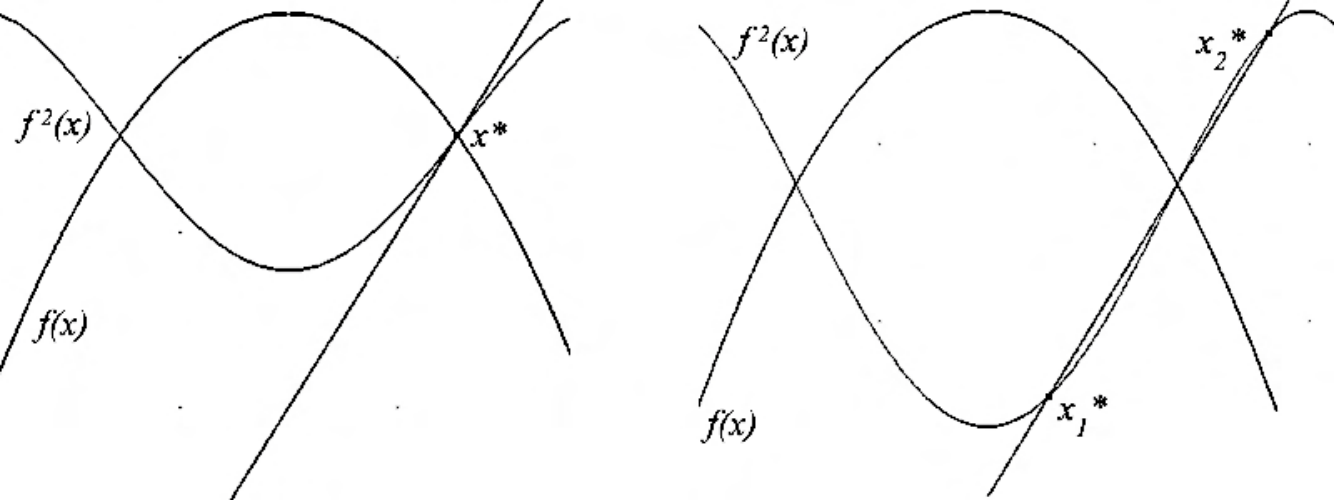
Let us now set $\mu=3-\varepsilon$ . Then $x^{*}=\frac{\mu-1}{\mu}$ is a stable fixed point with slope $f_{\mu}^{\prime}(x^{*})=\varepsilon-1$ . Correspondingly, the composition $f_{\mu}\circ f_{\mu}$ has also a fixed point there, with slope $(f_{\mu}\circ f_{\mu})^{\prime}(x^{*})=(\varepsilon-1)^{2}<1$ , again stable. Let now $\mu=3+\varepsilon$ . Then $x^{*}=\frac{\mu-1}{\mu}$ is unstable, with slope $f_{\mu}^{\prime}(x^{*})=-\varepsilon-1<-1$ . The same fixed point for the composition has then slope $(f_{\mu}\circ f_{\mu})^{\prime}(x^{*})=(\varepsilon+1)^{2}>1$ , and it is also unstable. Furthermore, as depicted in Figure 7, by continuity a couple of fixed points are created to the left and to the right of $x^{*}$ , and it is easy to see that they are stable.

The above reasoning seems to be applicable not only when going from period-one to period-two, but every time we double the period of the attractive cycle. We have already seen that for larger $\mu$ there exists an attractive four-cycle. It is worth plotting the bifurcation diagram for the logistic map, that indicates for any $\mu$ the set to which the motion is attracted. Looking at Figure 8 we see that at several points $\mu_{0},\mu_{1},\dots,\mu_{n},\dots$ a bifurcation occurs, where the number of attractive points doubles (i.e. one goes from a $2^{n}$ -cycle to a $2^{n+1}$ one). As we discussed, $\mu_{0}=3$ , and one can see from the plot that $\mu_{1}\approx 3.45$ , $\mu_{2}\approx 3.55$ , etc.

Furthermore, these points seem to accumulate to some $\mu_{\infty}\approx 3.6$ after which the trajectory jumps wildly between many points. To better understand this, let us look at Figure 9. One sees that the Lyapunov exponent $\gamma(\mu)$ is smaller than zero in presence of a $2^{n}$ -cycle, and vanishing at the bifurcation point as it should. However, for $\mu>\mu_{\infty}$ one sees that $\gamma(\mu)>0$ which signals the beginning of chaotic behavior¹⁰¹⁰ 10 For $\mu$ even larger there exists some interval where the behavior is back to periodic, with $\gamma(\mu)<0$ . These are the so-called periodic-windows, which we will not discuss here.. It is also interesting to notice that between any couple of bifurcation points there is (by continuity) a point where $\gamma(\tilde{\mu}_{n})=-\infty$ , with $\mu_{n-1}<\tilde{\mu}_{n}<\mu_{n}$ . This happens when one of the points in the cycle is the maximum $x=1/2$ , and we will then say that there the system has $2^{n}$ -superstable cycle.

We are not interested in what happens when $\mu>\mu_{\infty}$ . What is important to us, and we have established numerically, is that there is a sequence of period-doubling bifurcations at $\mu_{n}$ and, correspondingly, a sequence of superstable $2^{n}$ -cycles at $\tilde{\mu}_{n}$ , that converge to some $\mu_{\infty}$ .

$j$	$\tilde{\mu}_{j}$	$\delta_{j}$
0	3.00000000 $\dots$
1	3.44948974 $\dots$	4.751
2	3.54409035 $\dots$	4.656
3	3.56440726 $\dots$	4.668
4	3.56875941 $\dots$	4.668
5	3.56969160 $\dots$	4.669
6	3.56989125 $\dots$	4.669
7	3.56993401 $\dots$	4.668
8	3.56994317 $\dots$	4.667
9	3.56994514 $\dots$	4.671
10	3.5699455573883578	4.673
11	3.5699456473525193	4.66955
12	3.5699456666186404	4.66966
13	3.5699456707444445	4.66935
14	3.5699456716280371	4.66917
15	3.5699456718175778

Table 1: Values of

{\mu}_{j}

and

\delta_{j}

$n$	$\tilde{\mu}_{n}$	$d_{n}$	$\alpha_{n}$
1	3.236067977	-0.190983	-2.68555
2	3.498561698	0.0711151	-2.52528
3	3.554640862	-0.028161	-2.50880
4	3.566667379	0.0112250	-2.50400
5	3.569243531	-0.004482	-2.50316
6	3.569795293	0.0017908	-2.50296
7	3.569913465	-0.000715	-2.50295
8	3.569938774	0.0017908	-2.50293
9	3.569944194	-0.0007155	-2.50293

Table 2: Values of

\tilde{\mu}_{n}

d_{n}

and

\alpha_{n}

It is possible to compute numerically (e.g. by Newton’s method) the values of the first few $\mu_{n}$ ’s to a good precision. These are written in Table 2, and it is not hard to see that the sequence $\mu_{n}\to\mu_{\infty}\approx 3.5699$ converges, at least approximately, geometrically. We will call the number

\delta=\lim_{n\to\infty}\frac{\mu_{n}-\mu_{n-1}}{\mu_{n+1}-\mu_{n}}\approx 4.669201609\,,

(2.70)

Feigenbaum’s $\delta$ .¹¹¹¹ 11 It is interesting how Mitchell Feigenbaum found this rate of convergence; he was studying the sequence $\mu_{n}$ on a pocket calculator, and needed to guess the next bifurcation point as well as he could in order not to waste computer time. In doing so, he realized that the convergence was geometric. Notice that $\frac{\mu_{n}-\mu_{n-1}}{\mu_{n+1}-\mu_{n}}$ is not exactly equal to $\delta$ when $n$ is finite. Clearly the same rate dictates the convergence of $\tilde{\mu}_{n}$ as well.

Looking back at Figure 8 we see that the constant $\delta$ dictates the horizontal scale in the sequence of bifurcations. Clearly enough, there is also a vertical scale: in fact, after each bifurcation, the couple of new attractive points that are generated spread out in a $\sf C$ -shaped figure¹²¹² 12 Or $\sf U$ -shaped: in fact historically this goes under the name of $\sf U$ -sequence. as $\mu$ increases. The size of this $\sf C$ shrinks bifurcation after bifurcation, and it makes a lot of sense to suspect that it does so geometrically. The “size” $d_{n}$ can be defined as the distance between two neighboring points in a superstable cycle. This can be found by looking at the intersection of the bifurcation sequence with the line $x=x_{max}=1/2$ , as depicted in Figure 10.

In Table 2 the first few values of $d_{n}$ , as found numerically, are written. Indeed they converge geometrically, and one can define Feigenbaum’s $\alpha$ as

\alpha=\lim_{n\to\infty}\frac{d_{n}}{d_{n+1}}\approx-2.502907875\,,

(2.71)

which is negative because we keep into account the sign of $d_{n}$ , see Figure 10.

Universality
So far we have established that a certain family of maps of the interval into itself exhibits a sequence of period-doubling bifurcations, with geometric rate tending to $\delta\approx 4.669$ , leading to a chaotic behavior. What makes this story more interesting is that this behavior is common to many maps as well as real-world systems, i.e. it is, at least to some extent, universal.

In fact, one can check numerically that the same sequence of period-doubling bifurcations occurs for dynamical systems defined by the maps on $I=[0,1]$

	$\displaystyle f_{\mu}(x)$	$\displaystyle=$	$\displaystyle\mu\,(1-x^{2})(2x-x^{2})\,,\quad\quad 0\leq\mu\leq\frac{9}{16}\,,$
	$\displaystyle f_{\mu}(x)$	$\displaystyle=$	$\displaystyle\mu\,\sin(\pi x)\,,\quad\quad\quad\quad\quad\quad\quad 0\leq\mu\leq 1\,,$		(2.72)

as well as many others. What is more remarkable, the bifurcations points $\mu_{n}$ converge geometrically to some $\mu_{\infty}$ with a rate that tends to $\delta\approx 4.669$ . This happens also for dynamical systems of different kind, such as Mandelbrot’s set, or Rössler’s system of ODEs, see e.g. [20].

Furthermore, and what is more important from a physicist’s perspective, the period-doubling cascade towards chaos occurs also in real-world systems. For instance, let us consider a fluid-dynamics experiment of Rayleigh-Bénard convection, following Libchaber and Maurer [26].

Consider a box containing a fluid. The bottom of the box is kept at temperature $T$ , whereas the top is kept at $T+\Delta T$ . The temperature difference (or rather a related dimensionless quantity called Rayleigh’s number) is the external parameter that the experimenter may vary. When the temperature difference is small, heat is conduced to the colder upper surface. However, increasing the gradient, the familiar convective motions are generated. These consists of several counter-rotating cylinders that drive steadily the hotter fluid upwards.¹³¹³ 13 In practice, in order to obtain a stable enough convective motion, great care has to be taken in setting the experiment, such as picking appropriate shape and dimension of the box, and of course an appropriate fluid. Further increasing $\Delta T$ leads to a more complicated dynamics of the fluid: the heat flow is not steady any more, but fluctuates, as it can be seen by measuring the time-evolution of the local temperature at a given point in the upper surface.

This is a discrete-time dynamical system¹⁴¹⁴ 14 In fact, it makes sense to make measurements with time scales that are large with respect to the ones of the microscopic degrees of freedom.: $\Delta T$ plays the role of $\mu$ , and the oscillations of the local temperature the role of $\Phi^{n}(x)$ . What was found then is that, as one increases $\Delta T\sim\mu$ , one goes from the steady temperature (fixed point) to a two-cycle, then to a four-cycle, and so on. Even more strikingly, the period-doubling bifurcations occur geometrically with rate $4.4\pm 0.1$ compatible with $\delta$ . This has been shown to occur in a number of experiments in hydrodynamics [26, 27, 28, 29, 30], electronics [31, 32, 33, 34], charged gases [35] and chemistry [36].

It is worth pointing out that obtaining these experimental results is quite hard. On top of difficulties such as suppressing the noise and avoid generating chaotic behaviour due to other kind of turbulence, a key obstacle is that (due to the geometric progression) it is in practice possible to measure only the first few bifurcations. On the other hand, $\frac{\mu_{n}-\mu_{n-1}}{\mu_{n+1}-\mu_{n}}$ will approach $\delta$ only asymptotically. This makes these results even more remarkable.

Of course, the word “universal” should be taken with a pinch of salt. The maps (2.72) are not terribly general, and indeed they share some features with the logistic map:

1.

$f_{\mu}(x)$ is regular¹⁵¹⁵ 15 All our examples are analytic functions, which is a very strong requirement. We will not go into the details of how regular we need $f_{\mu}(x)$ to be..
2.

$f_{\mu}(x)$ is unimodal, i.e. it has one maximum $x_{max}$ and satisfies

$f^{\prime}_{\mu}(x)>0\,,\quad x<x_{max}\,\quad\quad\&\quad\quad f^{\prime}_{\mu}(x)<0\,,\quad x>x_{max}\,.$ (2.73)
3.

$f_{\mu}(x)$ has a quadratic maximum

$f^{\prime\prime}_{\mu}(x_{max})<0\,.$ (2.74)

It turns out that these requisites are indeed necessary. It is reasonable to require some kind of regularity, since we used it in the previous section to explain period-doubling. Let us consider the “tent” map of figure Figure 12, defined by

f_{\mu}(x)=\begin{cases}\mu\,x&x\leq 1/2\\ \mu(1-x)&x>1/2\end{cases}\,,\quad\quad 0\leq\mu\leq 2\,.

(2.75)

It is an unimodal map, but it is not differentiable at $x=1/2$ . In fact, since it is piecewise linear, its Lyapunov exponent is simply $\gamma=\log\mu$ so that the transition to chaos happens abruptly at $\mu=1$ with no period-doubling bifurcations. As for unimodality, it is also quite clear that a very general $f_{\mu}(x)$ with many maxima and minima may have a richer dynamics than the simpler examples we considered. As for the third requirement, it is hard to justify it a priori, and we will take it as an “experimental” evidence. What turns out is that maps that satisfy all requisites but have a maximum of higher order show the same period-doubling cascade, but with different universal constants in place of $\delta$ and $\alpha$ . For instance, if we were to consider a family $f_{\mu}$ with quartic maximum, we would find $\alpha\approx-1.69$ and $\delta\approx 7.28$ .¹⁶¹⁶ 16 Accurate values of such constants can be found e.g. in [37].

In the next section we will see how all these features can be explained in a “renormalization group” framework, which also yields quantitative predictions for $\delta$ and $\alpha$ .

2.3.3 Renormalization group for dynamical systems

In this section we will discuss how the universal behavior of period-doubling bifurcations can be explained in terms of renormalization group (RG) techniques. In this context, both words “renormalization” and “group” make little sense (to be fair, this name is a bit misleading in practically any context). They just indicate a rather general set of ideas of broad application, from quantum field theory to the physics of phase transitions.

Heuristic
We are concerned with several one-parameter families of maps $f_{\mu}$ of the interval $I$ into itself that exhibit similar period-doubling cascade of bifurcations. It makes sense to consider the space ${\cal{U}}$ of all maps with “good properties”,

{\cal{U}}=\{f:\ I\to I\,,\quad f\ {\rm regular,\ unimodal\ and\ with\ quadratic\ tip}\}\,.

(2.76)

Observe that the families $\{f_{\mu}\}\subset{\cal{U}}$ are curves in ${\cal{U}}$ . Clearly ${\cal{U}}$ is a subset of some space of functions, and to proceed rigorously further formalization (e.g. on the metric of this space) would be needed; here we will be qualitative.

Let us chose explicitly $I$ . Earlier we picked $I=[0,1]$ , but to better keep track of the maximum of $f_{\mu}(x)$ we will set $I=[-1,1]$ in such a way that the maximum is in $x=0$ and takes value $f_{\mu}(0)=1$ ; we further restrict to even maps to simplify the figures and the discussion. A typical map is shown in Figure 12.

To single out the fundamental characteristics of the universal behavior, it is easier to think in terms of superstable maps: we have that, for any $n=1,2,\dots$ at $\mu=\tilde{\mu}_{n}$ there exists a superstable map of period $2^{n}$ , and of characteristic size $d_{n}$ . The convergence of $\tilde{\mu}_{n}\to\mu_{\infty}$ has universal rate $\delta$ , whereas the one of $d_{n}\to 0$ has rate $\alpha$ .

Therefore, universality should emerge as a property of ${\cal{U}}$ under the action of some “renormalization” operator $\mathfrak{R}:{\cal{U}}\to{\cal{U}}$ . This operator

•

should relate maps with a $2^{n}$ -cycle to maps with a $2^{n-1}$ cycle,
•

should relate superstable maps to superstable maps, up to a rescaling of $\alpha$ .

The first property suggests that it must be $\mathfrak{R}(f)\sim f\circ f$ , which however is not an operator on ${\cal{U}}$ . In fact, it is easy to see that if $f(x)$ is unimodal, $f\circ f(x)$ is not. It is clear that some kind of rescaling is needed.

A generic map $f\in{\cal{U}}$ has its minimum on $I$ exactly at the boundaries of the interval. Looking at Figure 12, define

a=-f(1)\,,\quad\quad b=f(a)\,.

(2.77)

With a drawing, one can convince oneself that the following inclusions hold

f([-1,1])=[-a,1]\,,\quad f([-a,a])=[b,1]\,,\quad f([b,1])=[-a,f(b)]\subset[-a,a]\,,

(2.78)

provided that one has

0<a<b<1\,,\quad\quad f(b)<a\,.

(2.79)

In this case therefore one has that

f\circ f:\ [-a,a]\to[-a,a]\,.

(2.80)

Then, there is no problem to act with $\mathfrak{R}$ on $f$ , if we rescale all variables in an appropriate way (see Figure 13):

\mathfrak{R}(f)\,(x)=-\frac{1}{a}f\circ f(-a\,x)\,,

(2.81)

provided that (2.79) holds. In other words, (2.79) are conditions of $f\in{\cal{U}}$ to be in the domain of $\mathfrak{R}$ or, as sometimes it is said, for $f$ to be renormalizable.

Even if in general it is not immediate to see whether also $\mathfrak{R}(f)$ is in the domain of $\mathfrak{R}$ , for superstable maps things are easier. In fact, superstable maps are renormalizable, and if $f$ is a period- $2^{n}$ superstable map, then $\mathfrak{R}(f)$ is a period- $2^{n-1}$ superstable map, as it is easy to show. The values $\mu=\mu_{\infty}$ , where each family of maps gets to the onset of chaos, identify maps that have $2^{\infty}$ -period, and are therefore infinitely renormalizable.

It is now the time to change point of view, and start studying a new dynamical system, where ${\cal{M}}={\cal{U}}$ and $\Phi=\mathfrak{R}$ ; here we want to understand the orbits of the “points” $f\in{\cal{U}}$ (that are, in fact, functions in an infinite-dimensional space) under action of $\mathfrak{R}$ . This analysis may be more mathematically complicated and subtle than the previous ones, but we will reason by analogy with what we have seen until now.

Unfortunately, it is very hard to establish the properties of this infinite dimensional dynamical system, but a lot of progress can be made if we accept some conjectures, originally put forward by Feigenbaum [38, 39, 40], see also [41, 42].

1.

There is a fixed point $\phi^{*}\in{\cal{U}}$ , i.e. $\mathfrak{R}(\phi^{*})=\phi^{*}$ .
2.

The fixed point is hyperbolic, meaning that the derivative of the renormalization operator $\mathsf{R}=d\,\mathfrak{R}$ at $\phi^{*}$ has no eigenvalue of modulus one.
3.

Only one of its eigenvalues has modulus larger than one; we will call it $\delta$ .

Under these assumptions, it is reasonable to assume that there exists an unstable manifold ${\cal W}^{u}$ of dimension one which generalizes the eigenspace relative to $\delta$ , and a stable manifold ${\cal W}^{s}$ of codimension one, that generalizes the eigenspace of stable eigenvectors. Let us make an additional assumption.

4.

Let $\Sigma_{n}$ be the manifolds of period- $2^{n}$ superstable maps in ${\cal{U}}$ . Then ${\cal W}^{u}$ intersects $\Sigma_{1}$ transversally at $\phi^{*}_{0}\in{\cal W}^{u}\cap\Sigma_{1}$ .

We have already remarked that $\mathfrak{R}$ sends superstable maps into superstable maps. Therefore we have the inclusions

\mathfrak{R}^{n}(\Sigma_{n+1})\subset\Sigma_{1}\,,

(2.82)

and it is not hard to imagine that all the $\Sigma_{n}$ ’s will intersect transversally ${\cal W}^{u}$ , at points $\phi^{*}_{n-1}$ . It is also clear that the sequence $\phi^{*}_{n}$ converges geometrically to the fixed point $\phi^{*}$ , with rate $\delta$ . One can imagine that not only the points $\phi^{*}_{n}\to\phi^{*}$ , but also the manifolds $\Sigma_{n}$ accumulate toward the unstable manifold, and that their distance decreases geometrically with rate $\delta$ .

The whole picture is summarized in Figure 14. This also suggest how to explain the period-doubling cascade in a generic family of maps $\{f_{\mu}\}\subset{\cal{U}}$ . In fact, the sequence of bifurcations occurring at $\mu_{n}$ , or equivalently the sequence of superstable maps at $\tilde{\mu}_{n}$ can be described in terms of the behavior of the sequence of manifolds $\Sigma_{n}$ . We will return on this later, in order to make the relation with $\delta$ more quantitative.

As remarked, this whole discussion has been very qualitative. A rigorous treatment would bring us too far from the points of our discussions; the interested reader is invited to consult e.g. [43]. Here it is worth mentioning that, once Feigenbaum’s conjectures are accepted, it is not hard to prove that the scenario we described happens. What is much harder is to establish the existence of the hyperbolic fixed point. Remarkably, all this could be done rigorously [44, 45, 46, 47, 48]. Finally, let us stress that had we relaxed the condition that our maps are even, we would still have found a single hyperbolic fixed point $\phi^{*}$ , which turns out to be even.

Predictions from renormalization group
Now that we have formulated the RG ideas for maps on the interval, let us try to obtain some quantitative predictions out of them.

The first step is to find some information of the RG fixed point $\phi^{*}$ . We immediately encounter a difficulty: we must understand the role of $a$ which appears in the definition (2.81). It has to do with the rescaling of the $x$ -direction, and we know that for the fixed point this amounts to shrinking by (negative) $\alpha$ . This leads to the identification, at the fixed point

a=-1/\alpha\,.

(2.83)

This still leaves $\alpha$ undetermined. However, it is easy to see how this is fixed by the normalization of the maximum to $\phi^{*}(0)=1$ . Let us consider the ansatz for a symmetric $\phi^{*}(x)$

\phi^{*}(x)=1+\sum_{n=1}^{N}c_{n}\,x^{2n}+O(x^{2N+2})\,.

(2.84)

Plugging this into the fixed point equation

\phi^{*}(x)=\mathfrak{R}(\phi^{*})(x)=\alpha\,\phi^{*}(\phi^{*}(x/\alpha))\,,

(2.85)

we find e.g. for $N=3$ the solution

\alpha\approx-2.479\,,\quad c_{1}\approx-1.522\,,\quad c_{2}\approx 0.073\,,\quad c_{3}\approx 0.046\,.

(2.86)

Going to $N=6$ yields $\alpha\approx-2.502897$ , an estimate which turns out to be correct up to order $\sim 10^{-6}$ . Incidentally, the above procedure illustrates the importance of the order of the maximum, which is a crucial ingredient in our ansatz: a different choice would have lead to a different result for $\phi^{*}(x)$ .

Let us now try to find a more quantitative relation between $\delta$ and the sequence $\mu_{n}\to\mu_{\infty}$ for a family of maps $\{f_{\mu}\}\subset{\cal{U}}$ . It is convenient to introduce the short-hand notations

F(x)\equiv f_{\mu_{\infty}}(x)\,,\quad\quad\quad\varphi(x)\equiv\left.\frac{\partial\,f_{\mu}}{\partial\,\mu}\right|_{\mu_{\infty}}\!.

(2.87)

Then a function $f_{\mu}$ can be written, when $\mu$ is close to $\mu_{\infty}$ , as

f_{\mu}(x)\approx F(x)+(\mu-\mu_{\infty})\,\varphi(x)\,,

(2.88)

and similarly we can expand

\mathfrak{R}(f_{\mu})(x)\approx\mathfrak{R}(F)(x)+(\mu-\mu_{\infty})\,\mathsf{R}_{F}\cdot\varphi(x)\,.

(2.89)

Recall that $F$ lies exactly in the intersection ${\cal W}^{s}\cap\{f_{\mu}\}$ . Therefore, $\mathfrak{R}(F)\in{\cal W}^{s}$ is closer to $\phi^{*}$ than $F$ , and indeed due to the geometric convergence on the stable manifold, $\mathfrak{R}^{n}(F)\approx\phi^{*}$ after a few iterations. We can thus write

\mathfrak{R}^{n}(f_{\mu})(x)\approx\phi^{*}(x)+(\mu-\mu_{\infty})\,\mathsf{R}_{\phi^{*}}^{n}\cdot\varphi(x)\,.

(2.90)

Let us expand $\varphi$ on a basis of eigenfunctions of $\mathsf{R}_{\phi^{*}}$ ,

\varphi(x)=c_{\delta}\,\varphi_{\delta}(x)+\sum_{j}c_{j}\,\varphi_{j}(x)\,,

(2.91)

where we have distinguished the eigenfunction pertaining to $\delta$ . Since all eigenvalues except $\delta$ have modulus smaller than one, their eigenvectors $\varphi_{j}$ , $j\neq\delta$ are sent to zero by $\mathsf{R}_{\phi^{*}}^{n}$ . Only the eigenvector $\varphi_{\delta}$ of $\delta$ plays a role, so that we can eventually write

\mathfrak{R}^{n}(f_{\mu})(x)\approx\phi^{*}(x)+(\mu-\mu_{\infty})\,c_{\delta}\,\delta^{n}\,\varphi_{\delta}(x)\,.

(2.92)

Let us now specialize the above expression to the case $\mu=\tilde{\mu}_{n}$ , i.e. the case where the map is superstable of period $2^{n}$ , and evaluate it at $x=0$ . On the one hand, we have

\mathfrak{R}^{n}(f_{\tilde{\mu}_{n}})(0)=(f_{\tilde{\mu}_{n}})^{2^{n}}(0)=0\,,

(2.93)

due to the presence of the $2^{n}$ -cycle and the fact that $x=0$ is a point of the cycle. On the other hand we have

\phi^{*}(0)+(\tilde{\mu}_{n}-\mu_{\infty})\,c_{\delta}\,\delta^{n}\,\varphi_{\delta}(0)=\frac{1}{\alpha}+(\tilde{\mu}_{n}-\mu_{\infty})\,\delta^{n}\ \,c_{\delta}\,\kappa_{\delta}\,,

(2.94)

where we emphasized that $\kappa_{\delta}=\varphi_{\delta}(0)$ does not depend on $n$ . Therefore, at least up to higher order terms in $\tilde{\mu}_{n}-\mu_{\infty}$ it must be

(\tilde{\mu}_{n}-\mu_{\infty})\,\delta^{n}\approx-\frac{1}{\alpha\,c_{\delta}\,\kappa_{\delta}}={\rm const.}\,,

(2.95)

for any $\delta$ , which means exactly that the rate of convergence $\tilde{\mu}_{n}\to\infty$ is $\delta$ .

The only thing that remains to be done is to compute $\delta$ , using the explicit expression for the differential $\mathsf{R}$

\mathsf{R}_{\phi}\cdot\varphi(x)=-\frac{1}{a}\varphi\big(\phi(-a\,x)\big)-\frac{1}{a}\varphi(-a\,x)\,\phi^{\prime}\big(\phi(-a\,x)\big)\,,

(2.96)

and inserting the approximate result for $\phi^{*}(x)$ found by means of the power series expansion into the eigenvalue equation, we get

\alpha\,\varphi_{\delta}\big(\phi^{*}(x/\alpha)\big)+\alpha\,\varphi_{\delta}(x/\alpha)\,\phi^{*}{}^{\prime}\big(\phi(x/\alpha)\big)=\delta\,\varphi_{\delta}(x)\,,

(2.97)

and can be solved approximately by using an ansatz for $\varphi_{\delta}(x)$ too. The result, taking $N=6$ in the ansätze, is

\delta\approx 4.66914\,,

(2.98)

with an accuracy of order $\sim 10^{-5}$ with respect to the known result [37].

We have considered systems that are described by iterated maps on the interval (that is among the simplest dynamics one can imagine) where the experimenter is able to tune one parameter $\mu$ ; some class of these systems exhibit similar properties as the parameter approaches a critical value $\mu_{\infty}$ . We have explained this by using the properties of the renormalization of operator $\mathfrak{R}$ .

What is the physical interpretation of $\mathfrak{R}$ ? When we are looking at the dynamics, $\mathfrak{R}$ operates a rescaling of the time-scale ( $f\mapsto f\circ f$ ) together with a rescaling of the $x$ -scale. In this sense it is similar to Kadanoff’s coarse-graining transformation [49]: acting with the renormalization operators corresponds to changing the description of the problem, “zooming out” in such a way as to preserve the interesting (universal) properties of the dynamics.

In the language of statistical physics, we would say that $\mu$ plays the role of some adjustable “knob” (temperature, external magnetic field, etc.), and that at $\mu_{\infty}$ a phase transition occurs. The divergence of the correlation length in our case is mimicked by the appearance of an infinite-period cycle. All the systems at the phase transitions are points on the stable manifold ${\cal W}^{s}$ , and due to this they are very similar. In fact, under the action of $\mathfrak{R}$ , all these points get to the fixed point $\phi^{*}$ , so that the properties invariant under $\mathfrak{R}$ (the large scale properties, in a statistical system) are common to all of them. We did not investigate at all what happens to our maps at $\mu_{\infty}$ (to avoid the complications of chaotic systems), but it is indeed possible to single out several universal properties.

The role played by $\delta$ is that of a relevant eigenvalue, and $\varphi_{\delta}(x)$ is a relevant direction at the fixed point. This means that if we perturb $\phi^{*}(x)$ by something proportional to $\varphi_{\delta}(x)$ , acting with $\mathfrak{R}$ will drive us away from the fixed point. Notice that in Figure 14 the stable manifold separates ${\cal{U}}$ in two regions. Maps on either side of the ${\cal W}^{s}$ will have different behavior under $\mathfrak{R}$ and therefore different properties. We have seen that all the maps “below” the stable manifold ( $\mu<\mu_{\infty}$ ) are periodic, with negative Lyapunov exponent, whereas indeed maps “above” ${\cal W}^{s}$ will yield chaotic behavior. Again this is in analogy with what happens in statistical systems, where the position in parameter space of a theory determines its large-scale properties.

2.4 Series convergence and Borel summability

Before going to the core of our review we will take a moment to discuss the status of the perturbative expansion in QFT. This expansion is obtained by performing a Taylor expansion of the interaction, and then commute the sum with the Gaussian integral to obtain a series indexed by combinatorial maps:

	$\displaystyle\langle 1\rangle$	$\displaystyle=$	$\displaystyle\int d\mu_{C}\;\;e^{-\frac{\lambda}{4!}\int d^{d}x\phi^{4}(x)}$		(2.99)
		$\displaystyle=$	$\displaystyle\sum_{n=0}^{\infty}\frac{1}{n!}\frac{(-\lambda)^{n}}{(4!)^{n}}\sum_{\text{labelled combinatorial maps with n vertices}}A(M)\;.$		(2.100)

The problem of the perturbative series is that it is badly divergent: as there are $(4n-1)!!$ labelled combinatorial maps with $n$ vertices, the series behaves like

\displaystyle\sum_{n=0}^{\infty}\frac{1}{n!}\frac{(-\lambda)^{n}}{(4!)^{n}}(4n-1)!!=\sum_{n=0}^{\infty}\frac{1}{n!}\frac{(-\lambda)^{n}}{(4!)^{n}}\frac{(4n)!}{2^{2n}(2n)!}

(2.101)

which has zero radius of convergence.

The root of the problem is that we performed an expansion in $\lambda$ around $\lambda=0$ . However the original integral is convergent for $\lambda>0$ but it is divergent for $\lambda<0$ . The partition function $\langle 1\rangle$ is analytic in some domain in the complex plane outside the negative real axis. Hence $\lambda=0$ belongs to the boundary of the analyticity domain of $\langle 1\rangle$ . A Taylor expansion around a point belonging to the boundary of analyticity domain of some function is not absolutely convergent.

A legitimate question is therefore how much of the information we extract from the perturbative expansion is of any relevance to QFT? Does a divergent Taylor series encode any relevant information about the original function? The answer for a smooth function of a real variable in general is no: an asymptotic series does not encode any relevant information (the typical example is the function $f(\lambda)=0$ for $\lambda\leq 0$ and $f(\lambda)=e^{-\frac{1}{\lambda}}$ for $\lambda>0$ whose asymptotic series at $\lambda=0$ is $0$ ).

Only under very special circumstances does a divergent Taylor series encode some information about the function it is coming from: in fact under certain assumptions such a series can uniquely fix the function. Fortunately for us, this is the case in QFT: in many cases, while divergent, the perturbative series is Borel summable.

Theorem 2.15 (Nevanlinna-Sokal, [9])

A function $f(\lambda,N)$ with $\lambda\in\mathbb{C}$ and $N\in\mathbb{R}_{+}$ is said to be Borel summable in $\lambda$ uniformly in $N$ if

•

$f(\lambda,N)$ is analytic in a disk $\Re{(\lambda^{-1})}>R^{-1}$ with $R\in\mathbb{R}_{+}$ independent of $N$ .

•

$f(\lambda,N)$ admits a Taylor expansion at the origin

\displaystyle f(\lambda,N)=\sum_{k=0}^{r-1}f_{N,k}\lambda^{k}+R_{N,r}(\lambda)\;,\qquad|R_{N,r}(\lambda)|\leq K\sigma^{r}r!|\lambda|^{r}\;,

(2.102)

for some constants $K$ and $\sigma$ independent of $N$ .

If $f(\lambda,N)$ is Borel summable in $\lambda$ uniformly in $N$ then

B(t,N)=\sum_{k=0}^{\infty}\frac{1}{k!}f_{N,k}t^{k}

is an analytic function for $|t|<\sigma^{-1}$ which admits an analytic continuation in the strip $\{z|\;|\Im z|<\sigma^{-1}\}$ such that $|B(t,N)|\leq Be^{t/R}$ for some constant $B$ independent of $N$ and $f(\lambda,N)$ is represented by the absolutely convergent integral

\displaystyle f(\lambda,N)=\frac{1}{\lambda}\int_{0}^{\infty}dt\;B(t,N)e^{-\frac{t}{\lambda}}\;.

(2.103)

That is the Taylor expansion of $f(\lambda,N)$ at the origin is Borel summable, and $f(\lambda,N)$ is its Borel sum. The set $\{\lambda|\Re{(\lambda^{-1})}>R^{-1},R\in\mathbb{R}_{+}\}$ is a disk (called a Borel disk) in the complex plane with center at $\frac{R}{2}$ and of radius $\frac{R}{2}$ (see Figure 15) as, denoting $\lambda=\frac{R}{2}+ae^{\imath\gamma}$ ,

\displaystyle\Re{(\lambda^{-1})}>R^{-1}\Leftrightarrow\frac{R^{2}}{4}>a\;.

(2.104)

Figure 15: A Borel disk.

Borel summability provides a uniqueness criterion: if a series is the Taylor expansion of a Borel summable function $f(\lambda,N)$ at $\lambda=0$ , then $f(\lambda,N)$ is the unique Borel summable function whose Taylor series is the original series. This is the case of the $\phi^{4}_{d}$ model and of QFT in general.

In fact Borel summability allows to recover $e^{\frac{1}{\lambda}}$ effects. Although such effects cannot be captured by the perturbative series, they are recovered by analytic continuation. In fact one expects a $e^{\frac{1}{\lambda}}$ behaviour for $\lambda\in\mathbb{R},\lambda<0$ : this is the typical contribution of “instantons” (that is non trivial solutions of the classical equations of motion) which exist for $\lambda<0$ . The instanton contributions are recovered by first Borel summing the perturbative series (which yields a convergent expression for $\Re\lambda>0$ ) and then analytically continuing to the $\Re\lambda<0$ half complex plane. The negative real axis is a cut and the partition function $\langle 1\rangle$ (or more precisely its logarithm, the free energy) can be continued on a Riemann surface. The discontinuity of this analytic continuation at the cut captures the instanton contributions.

3 Renormalization essentials

We refer loosely to [6] and references therein for this section. Quantum transition probabilities are represented by a “sum over histories” of particles, i.e. a functional integral. Expanding this functional integral in term of the number of collisions or interactions of the particles leads to perturbative quantum field theory, indexed by combinatorial maps. In these maps, the particle collisions or interactions are represented by vertices. The propagation of particles is represented by the edges joining these vertices. Any correlation is computed by the weighted sum over infinitely many maps. The maps to be summed and the weights (a.k.a. Feynman amplitudes) are determined from the classical action of the theory by the Feynman rules.

The simplest functional integrals are the one describing free theories, that amount to considering Gaussian measures.

3.1 Gaussian measures

A finite dimensional centered normalized Gaussian measure $d\mu_{C}$ is defined through its covariance. Consider a finite dimensional space ${\mathbb{R}}^{N}$ . The field $\phi$ is a function $\phi:\{1,2,\dots N\}\to\mathbb{R}$ . Let $C$ be a symmetric, positive definite, $N$ by $N$ matrix . The naive definition of the centered normalized Gaussian measure of covariance $C$ is

\displaystyle d\mu_{C}=\frac{1}{(2\pi)^{N/2}\sqrt{\det C}}\;\;e^{-\frac{1}{2}\sum_{i,j}\phi_{i}(C^{-1})_{ij}\phi_{j}}d^{N}\phi,

(3.1)

so that $\int d\mu_{C}=1$ . Taking eq. (3.1) as the definition of Gaussian measures has two drawbacks:

•

eq. (3.1) is well defined only if $C^{-1}$ exists.
•

more importantly, if one tries to generalize this definition for $\phi$ a genuine field $\phi:\mathbb{R}^{d}\to\mathbb{R}$ , one runs into troubles: the functional measure involves a factor $\prod_{x\in\mathbb{R}^{d}}d\phi(x)$ , which is an ill defined infinite product of Lebesgue measures.

This is clearly not a solid starting point for the study of QFT. The correct starting point is the following. Any function can be approximated by polynomials, hence probability measures are characterized by the expectations of polynomials in the random variables (the moments of the measure). For Gaussian measures, this can be rendered rigorous by using Minlos’ Theorem [5] and the general theory of Gaussian processes. For any operator $C:L^{2}(\mathbb{R}^{d})\to L^{2}(\mathbb{R}^{d})$ , with kernel $C(x,y)$ , we define

Definition 3.1

The centered, normalized Gaussian measure of covariance $C$ , $\mu_{C}$ is defined by its moments

\displaystyle\int d\mu_{C}(\phi)\;\prod_{i=1}^{n}\phi(x_{i})=\begin{cases}1&\text{if }n=0\\ 0&\text{if }n\text{ is odd}\\ \sum_{G}\prod_{\ell\in G}C(x_{i},x_{j})\;&\text{if }n(\neq 0)\text{ is even}\end{cases}\;,

(3.2)

where $G$ denotes all the pairings of $n$ elements into pairs $\ell=(i,j)$ (that is distinct partitions of the set $1\dots n$ into subsets of two elements).

The moments of a Gaussian measure admit a simple graphical representation in Feynman diagrams. We represent the insertions $\phi(x_{1}),\dots\phi(x_{n})$ as vertices, and the pairs $\ell$ as edges connecting the vertices. A pairing $G$ is thus a Feynman graph (a combinatorial map).

The Euclidean quantum field theory of a free scalar field amounts to studying the (normalized) functional measure

\displaystyle d\mu_{C}(\phi)\;,\;\;C(x,y)=\Bigl(\frac{1}{-\Delta+m^{2}}\Bigr)(x,y)=\int_{0}^{\infty}\frac{d\alpha}{(4\pi\alpha)^{d/2}}\;\;e^{-\frac{|x-y|^{2}}{4\alpha}-\alpha m^{2}}\;.

(3.3)

The QFT predictions are the moments of this measure

\Big\langle\phi(x_{1})\cdots\phi(x_{k})\Big\rangle=\int d\mu_{C}\;\phi(x_{1})\cdots\phi(x_{k})\;,

(3.4)

which follow from the definition 3.1 and make perfect sense for $\phi(x)$ a function on $\mathbb{R}^{d}$ . In particular the apparent problem that $\prod_{x\in\mathbb{R}^{d}}d\phi(x)$ is an ill defined infinite product of Lebesgue measures simply does not exist.

The moments can be obtained as the functional derivatives of the generating functional $Z[J]$

	$\displaystyle Z[J]\equiv\int d\mu_{C}\;e^{\int d^{d}x\,J(x)\phi(x)}\;,$		(3.5)
	$\displaystyle\Big\langle\phi(x_{1})\cdots\phi(x_{k})\Bigr\rangle=\frac{\delta}{\delta J(x_{k})}\cdots\frac{\delta}{\delta J(x_{1})}Z[J]\Big\|_{J=0}\;.$		(3.6)

The generating functional can be evaluated exactly in this case, by performing the Gaussian integral

	$\displaystyle Z(J)=\sum_{n\geq 0}\frac{1}{n!}\int d^{d}x_{1}\dots d^{d}x_{n}\;J(x_{1})\dots J(x_{n})\int d\mu_{C}\;\phi(x_{1})\dots\phi(x_{n})$		(3.7)
	$\displaystyle=\sum_{n\geq 0}\frac{1}{n!}\int d^{d}x_{1}\dots d^{d}x_{n}\;J(x_{1})\dots J(x_{n})\sum_{G}\prod_{\ell\in G}C(x_{a(\ell)},x_{b(\ell)})$		(3.8)
	$\displaystyle=\sum_{p\geq 0}\frac{1}{(2p)!}(2p-1)!!\Bigl(\int d^{d}xd^{d}yJ(x)C(x,y)J(y)\Bigr)$		(3.9)
	$\displaystyle=e^{\frac{1}{2}\int d^{d}xd^{d}yJ(x)C(x,y)J(y)}\;,$		(3.10)

where we used the fact that there are $(2p-1)!!=\frac{(2p)!}{2^{p}p!}$ pairings of $2p$ labels. The two-point Schwinger function is just the free Euclidean propagator¹⁷¹⁷ 17 Of course, if we wanted to consider the Minkowskian theory, we would have to worry about a prescription to obtain the correct Green’s function by analytic continuation.. Similarly, we can find the explicit expression for all correlations (3.4), which can be expressed by the familiar Feynman diagrams. For a Gaussian measure, it is immediate to see that the connected moments and their generating functional are:

	$\displaystyle e^{W[J]}\equiv Z[J]\;,$		(3.11)
	$\displaystyle\Big\langle\phi(x_{1})\cdots\phi(x_{k})\Bigr\rangle_{c}=\frac{\delta}{\delta J(x_{k})}\cdots\frac{\delta}{\delta J(x_{1})}W(J)\Big\|_{J=0}\;.$		(3.12)

Here the connected moments are particularly simple: the only non-vanishing one is the two-point connected moment which equals the covariance itself. For general (non Gaussian) measures, the covariance is defined as the connected two point function, and as we will prove in the next section the generator of connected moments is also given by (3.11).

For an arbitrary function $F(\phi)$ ,

	$\displaystyle\int d\mu_{C}(\phi)F(\phi)=\int d\mu_{C}(\phi)\Bigg[F\bigl(\frac{\delta}{\delta J}\bigr)e^{\int_{x}J(x)\phi(x)}\Bigg]\Bigg\|_{J=0}$		(3.13)
	$\displaystyle=\Bigg[F\bigl(\frac{\delta}{\delta J}\bigr)\int d\mu_{C}(\phi)e^{\int_{x}J(x)\phi(x)}\Bigg]\Bigg\|_{J=0}=\Bigg[F\bigl(\frac{\delta}{\delta J}\bigr)e^{\frac{1}{2}\int_{xy}J(x)C(x,y)J(y)}\Bigg]\Bigg\|_{J=0}$		(3.14)
	$\displaystyle=\Bigg[e^{\frac{1}{2}\int_{xy}\frac{\delta}{\delta\phi(x)}C(x,y)\frac{\delta}{\delta\phi(y)}}F(\phi)\Bigg]\Bigg\|_{\phi=0}\;.$		(3.15)

This expression of the normalized Gaussian measure is by far the most useful for explicit computations. As a direct application we have the following lemma.

Lemma 3.1 (Split of a normalized Gaussian Measure)

Consider a normalized Gaussian measure $\mu_{C}(\phi)$ . For any decomposition of the covariance $C=C_{1}+C_{2}$ there exists an associated decomposition of the field $\phi(x)=\phi_{1}(x)+\phi_{2}(x)$ , with the fields $\phi_{1}$ and $\phi_{2}$ independent distributed on Gaussians with covariances $C_{1}$ and $C_{2}$ such that

\displaystyle d\mu_{C}(\phi)=d\mu_{C_{1}}(\phi_{1})d\mu_{C_{2}}(\phi_{2})\;.

(3.16)

Proof: We have

	$\displaystyle\Bigg[e^{\frac{1}{2}\int_{xy}\frac{\delta}{\delta\phi_{1}(x)}C_{1}(x,y)\frac{\delta}{\delta\phi_{1}(y)}+\frac{1}{2}\int_{xy}\frac{\delta}{\delta\phi_{2}(x)}C_{2}(x,y)\frac{\delta}{\delta\phi_{2}(y)}}F(\phi_{1}+\phi_{2})\Bigg]\Bigg\|_{\phi_{1}=\phi_{2}=0}$		(3.17)
	$\displaystyle=\Bigg[e^{\frac{1}{2}\int_{xy}\frac{\delta}{\delta\phi_{1}(x)}C_{1}(x,y)\frac{\delta}{\delta\phi_{1}(y)}}\Bigg[e^{\frac{1}{2}\int_{xy}\frac{\delta}{\delta\phi(x)}C_{2}(x,y)\frac{\delta}{\delta\phi(y)}}F(\phi)\Bigg]\Bigg\|_{\phi=\phi_{1}}\Bigg]_{\phi_{1}=0}$		(3.18)
	$\displaystyle=\Bigg[e^{\frac{1}{2}\int_{xy}\frac{\delta}{\delta\phi_{1}(x)}C_{1}(x,y)\frac{\delta}{\delta\phi_{1}(y)}}\Bigg[e^{\frac{1}{2}\int_{xy}\frac{\delta}{\delta\phi_{1}(x)}C_{2}(x,y)\frac{\delta}{\delta\phi_{1}(y)}}F(\phi_{1})\Bigg]\Bigg]_{\phi_{1}=0}$		(3.19)
	$\displaystyle=\Bigg[e^{\frac{1}{2}\int_{xy}\frac{\delta}{\delta\phi_{1}(x)}[C_{1}(x,y)+C_{2}(x,y)]\frac{\delta}{\delta\phi_{1}(y)}}F(\phi_{1})\Bigg]_{\phi_{1}=0}\;.$		(3.20)

$\Box$

Another useful lemma is the following

Lemma 3.2

The measure

\displaystyle d\mu_{C}(\phi)\;\sqrt{\det(1-C^{-1}M)}\;e^{\frac{1}{2}\int_{x,y}\phi(x)M(x,y)\phi(y)}\;,

(3.21)

is also a normalized Gaussian measure and its covariance is

\displaystyle\bar{C}(x,y)=\Bigg(C\frac{1}{1-MC}\Bigg)(x,y)\;.

(3.22)

Proof: In self evident shorthand notations, the expectation of an arbitrary function of the field is

\displaystyle\sqrt{\det(1-C^{-1}M)}\;\Big[e^{\frac{1}{2}\frac{\delta}{\delta\phi}C\frac{\delta}{\delta\phi}}\;e^{\frac{1}{2}\phi M\phi}F(\phi)\Bigr]_{\phi=0}\;,

(3.23)

which rewrites

\displaystyle\Bigl[F\bigl(\frac{\delta}{\delta\phi}\bigr)\Bigl(e^{\frac{1}{2}\mathrm{Tr}[\ln(1-C^{-1}M)]}\;\;e^{\frac{1}{2}\frac{\delta}{\delta\phi}M\frac{\delta}{\delta\phi}}e^{\frac{1}{2}\phi C\phi}\Bigr)\Bigr]_{\phi=0}\;.

(3.24)

To evaluate

\displaystyle e^{\frac{1}{2}\frac{\delta}{\delta\phi}M\frac{\delta}{\delta\phi}}e^{\frac{1}{2}\phi C\phi}\;,

(3.25)

we note that this expression is a sum over graphs with labelled vertices. The graphs have two valent vertices (which bring a weight $\frac{C}{2}$ ), and edges (with weight M). Its logarithm is then a sum over connected graphs. The connected graphs can be

•

Cycles of length $p$ . The combinatorial factor of a cycle of length $p$ is $\frac{1}{p!}\frac{1}{2^{p}}(p-1)!2^{p-1}=\frac{1}{2p}$ and the amplitude is $\mathrm{Tr}[(MC)^{p}]$ .
•

Chains of length $p$ . The combinatorial factor of a chain of length $p$ is $\frac{1}{p!}\frac{1}{2^{p}}p!2^{p-1}=\frac{1}{2}$ , and its amplitude $\phi C(MC)^{p}\phi$ .

Thus

	$\displaystyle e^{\frac{1}{2}\frac{\delta}{\delta\phi}M\frac{\delta}{\delta\phi}}e^{\frac{1}{2}\phi C\phi}=e^{\sum_{p\geq 1}\frac{1}{2p}\mathrm{Tr}[(MC)^{p}]+\sum_{p\geq 0}\frac{1}{2}\phi C(MC)^{p}\phi}$		(3.26)
	$\displaystyle=e^{-\frac{1}{2}\mathrm{Tr}[\ln(1-C^{-1}M)]+\frac{1}{2}\phi C\frac{1}{1-MC}\phi}\;,$		(3.27)

and the lemma follows

$\Box$

3.2 Generating functionals

Let us review two generating functionals that are most useful in the study of the measures associated to QFTs.

3.2.1 The generating functional of connected graphs

We have already encountered this functional in the case of free theories. Here we prove that even for an interacting theory (3.11) expresses the generator of connected moments, i.e. of moments given by connected Feynman graphs. Let ${Z}$ be the formal power series which writes as a sum over graphs $G$ with $n(G)$ labelled vertices and with “amplitudes” $A(G)$ , depending on the graph $G$ but not on the labels:

\displaystyle{Z}=\sum_{G}\frac{1}{n(G)!}A(G)\;.

(3.28)

We want to see that if the amplitude of $G$ factors over its connected components, then

\displaystyle W\equiv\ln{Z}=\sum_{G_{c}}\frac{1}{n_{c}(G_{c})!}A(G_{c})\;,

(3.29)

where $G_{c}$ runs over the connected graphs with labelled vertices.

To see this, we list the connected graphs $G_{1}$ , $G_{2}$ , and so on. We denote $n_{1}$ , $n_{2}$ and so on the number of vertices of $G_{1}$ , $G_{2}$ , etc. Any graph $G$ has a unique decomposition $G=G_{1}^{q_{1}}\cup G_{2}^{q_{2}}\dots\cup G_{k}^{q_{k}}\dots$ . There are $\frac{n!}{\prod_{i}q_{i}!(n_{i}!)^{q_{i}}}$ distinct ways to distribute the $n$ labels of the vertices of $G$ into $q_{1}$ boxes of size $n_{1}$ , $q_{2}$ boxes of size $n_{2}$ , op to $q_{k}$ boxes of size $n_{k}$ , corresponding to the vertices of $G_{1}$ , $G_{2}$ , and so on. We therefore have

	$\displaystyle Z=\sum_{G}\frac{1}{n(G)!}A(G)=\sum_{G_{1}^{q_{1}}\cup G_{2}^{q_{2}}\dots\cup G_{k}^{q_{k}}\dots}\frac{1}{n(G)!}\prod_{c}\Bigl(A(G_{c})\Bigr)^{q_{c}}$
	$\displaystyle=\sum_{q_{1}\geq 0,\dots q_{k}\geq 0\dots}\frac{1}{(\sum_{c\geq 1}n_{c}q_{c})!}\prod_{c}\Bigl(A(G_{c})\Bigr)^{q_{c}}\;\;\frac{(\sum_{c\geq 1}n_{c}q_{c})!}{\prod_{i}q_{i}!(n_{i}!)^{q_{i}}}$
	$\displaystyle=\sum_{q_{1}\geq 0,\dots q_{k}\geq 0\dots}\frac{1}{\prod_{c}q_{c}!}\prod_{c}\Bigl(\frac{1}{n_{c}!}A(G_{c})\Bigr)^{q_{c}}$
	$\displaystyle=\sum_{q\geq 0}\frac{1}{q!}\Bigl(\sum_{c}\frac{1}{n_{c}!}A(G_{c})\Bigr)^{q}=e^{\sum_{c}\frac{1}{n_{c}!}A(G_{c})}\;.$

3.2.2 The quantum effective action

Another generating functional, which will be useful later on is the Legendre transform of $W[J]$ . We define the “effective field” $\varphi(x)$ as

\varphi(x)=\frac{\delta W[J]}{\delta J(x)}\;.

(3.30)

The above equation can be solved for $J$ as a function of $\varphi$ , $J_{\varphi}$ . The Legendre transform of $W[J]$ is then

	$\displaystyle\Gamma[\varphi]$	$\displaystyle=$	$\displaystyle\inf_{J}\left(-W[J]+\int d^{d}xJ(x)\varphi(x)\right)$		(3.31)
		$\displaystyle=$	$\displaystyle-W[J_{\varphi}]+\int d^{d}xJ_{\varphi}(x)\varphi(x)\;.$		(3.32)

Observe that in the free case, $J_{\varphi}$ can be found explicitly

\varphi(x)=\frac{\delta W[J]}{\delta J(x)}=\int d^{d}y\;C(x,y)J(y)\Rightarrow J_{\varphi}(x):=(-\Delta+m^{2})\varphi(x)\;.

(3.33)

The derivative of $\Gamma$ is

	$\displaystyle\frac{\delta\Gamma[\varphi]}{\delta\varphi(x)}=-\int d^{d}y\;\frac{\delta W}{\delta J(y)}\Big\|_{J_{\varphi}}\frac{\delta J_{\varphi}(y)}{\delta\varphi(x)}$		(3.34)
	$\displaystyle\qquad\qquad+\int d^{d}y\frac{\delta J_{\varphi}(y)}{\delta\varphi(x)}\varphi(y)+J_{\varphi}(x)=J_{\varphi}(x)\,.$		(3.35)

This is a constraint for the effective field: in absence of currents $\varphi(x)$ must solve a variational equation similar to the one for $S[\phi]$ in the classical theory. For this reason, $\Gamma[\varphi]$ is called the quantum effective action.

We have two complementary interpretations for $\Gamma$ : on the one hand, in a diagrammatic approach, it can be proven that $\Gamma$ can be obtained from the one particle irreducible (1PI) Feynman diagrams, ¹⁸¹⁸ 18 This was actually the way the effective action was originally defined [50], whereas the functional definition (3.31) was given in [51, 52, 53, 54]; see also [55] for a derivation of the $n$ -loop expansion of $\Gamma$ ..

We can also think of $\Gamma$ as given by an infinite series in $\varphi^{n}$ , whose coefficients depend on the loop integrals¹⁹¹⁹ 19 Actually, on the renormalized loop integrals, as it will be clearer later.. Such an expansion in effective vertices will be“semi-local”, since we are not just summing tree diagrams:

\Gamma[\varphi]=\sum_{n}\frac{1}{n!}\int d^{4}x_{1}\cdots d^{4}x_{N}\,\Gamma^{(n)}[x_{1},\dots,x_{N}]\varphi(x_{1})\cdots\varphi(x_{N}).

(3.36)

This gives a second interpretation: the full quantum theory generated by the action $S$ is equivalent to the classical (tree-level) theory for an action $S_{new}=\Gamma$ built out of the effective vertices. As a result we can write

\Gamma[\varphi]=S[\varphi]+\mathrm{quantum\ corrections}.

(3.37)

For more on this, see §16 in [53, 54] and §8 in [56].

If we go back to the free theory, we can explicitly substitute (3.33) in the definition of $W[J]$ to find that

\Gamma[\varphi]=\int d^{4}x\frac{1}{2}\varphi(x)\left(-\Delta+m^{2}\right)\varphi(x)\,.

(3.38)

This shows that a free theory, even after taking into account quantum corrections, just describes the propagation of noninteracting particles, as was already clear from (3.7). Furthermore, we see that

\frac{\delta^{2}\Gamma[\varphi]}{\delta\varphi(x)\,\delta\varphi(y)}=\frac{\delta J_{\varphi}(y)}{\delta\varphi(x)}=\left[\frac{\delta^{2}W[J]}{\delta J(x)\,\delta J(y)}\right]^{-1}\Bigl|_{J=J_{\varphi}}\;.

(3.39)

One also obtains from (3.31) that²⁰²⁰ 20 For a proof of this last expression, see [53, 54] §18, or [57] §2.5 where a different strategy is used: the above formula is taken as definition, and the familiar properties of $\Gamma$ are derived from it.

\displaystyle\exp\left(-\Gamma[\varphi]\right)

\displaystyle=\frac{1}{\mathcal{N}}\int\mathcal{D}\rho\,\exp\left\{-S[\rho+\varphi]+\int d^{d}x\frac{\delta\Gamma[\varphi]}{\delta\varphi(x)}\,\rho(x)\right\}

(3.40)

which can be taken as an alternative definition of $\Gamma[\varphi]$ .

3.3 Warm-up examples

Before tackling interacting QFTs on $\mathbb{R}^{d}$ , let us consider two simpler examples that illustrate how to work with generating functionals and their expansions.

3.3.1 The single point universe

Let us start with a point-like universe, hence "field theory in zero dimension". The field is then a random variable and we consider the one dimensional Gaussian measure of covariance $1$ , which can be written as

d\mu(\phi)=e^{-\phi^{2}/2}\frac{1}{\sqrt{2\pi}}d\phi.

(3.41)

The moments of this measure are

\bigl\langle\phi^{2p+1}\big\rangle=0\;,\qquad\bigl\langle\phi^{2p}\big\rangle=(2p-1)!!\;.

(3.42)

The Feynman graph representation pictures $(2p-1)!!$ as a sum over graphs. Each variable $\phi$ is pictured as a vertex with a "half-edge" or "field" hooked to it. The result of Gaussian integration is then expressed as a sum over all possible pairings between these fields. Each such pairing is represented as an edge between the corresponding vertices. The set $G$ of all vertices and edges is called the Feynman graph associated to the pairing. It is still quite trivial, as each connected component is made of a single edge and its two ends.

Figure 16: A contraction scheme on 6 fields.

Interactions are then added to the measure to make it non-Gaussian and lead to interesting Feynman graphs with vertices of degree higher than 1. To illustrate our purpose let us consider the following one dimensional integral

Z(\lambda)=\int_{-\infty}^{+\infty}e^{-\phi^{2}/2-\lambda\phi^{4}}d\phi\;

(3.43)

which is the partition function of the $\phi^{4}_{0}$ model. We choose to consider a $\lambda\phi^{4}$ perturbation of the Gaussian measure rather than the lower degree $\lambda\phi^{3}$ because the function $Z$ is then well defined as a convergent integral for $\lambda$ positive.

Expanding the exponential as a power series in the coupling constant $\lambda$ , and commuting sums and integrations without caring for convergence we get

Z(\lambda)=\sum_{n=0}^{\infty}\frac{(-\lambda)^{n}}{n!}(4n-1)!!\;.

(3.44)

Instead of considering $4n$ vertices of degree 1, we consider $n$ vertices, each of degree 4, hence with four half-edges or ‘fields" hooked, and the pairings now build up Feynman graphs (combinatorial maps) with $n$ vertices, each of degree 4. Such drawings can now be connected or not.

Figure 17: Vacuum Graphs with

n=1,2

At order $n=1$ we have 4 fields, hence $3$ combinatorial maps which all correspond to the same connected graph. At order $n=2$ we have 8 fields, hence $105$ combinatorial maps, which give three graphs, one made of two connected components, of weight $9$ , the two others connected, of weights 24 and 72.

If we compute the first two orders of $Z$ we have therefore

Z(\lambda)=1-3\lambda+\frac{105}{2}\lambda^{2}+O(\lambda^{3})\;,\qquad\log Z(\lambda)=1-3\lambda+\frac{96}{2}\lambda^{2}+O(\lambda^{3})

and we remark that 96= 24+72 is, as expected, the number connected maps with two four valent vertices.

The higher moments of the interacting measure

S_{N}=\frac{1}{Z(\lambda)}\int_{-\infty}^{+\infty}\phi^{N}e^{-\phi^{2}/2-\lambda\phi^{4}}d\phi\;,

(3.45)

are given by sums over all Feynman graphs (combinatorial maps) with $N$ external vertices of degree 1 and any number $n$ of internal vertices of degree 4. All these sums are divergent, but Borel summable.

3.3.2 Quantum field theory on a finite graph

The single-point universe was too simple an example to illustrate the role of graphs, contractions and combinatorics that are ubiquitous in QFT. To do so without introducing all of the QFT complications, let us now consider a universe with many points, made of a fixed finite graph $\Gamma$ , on which particles propagate and interact. This is obtained by the following generalization of the functional integral (3.43):

•

the field $\phi$ is replaced by a function $\phi:V(\Gamma)\to\mathbb{R}$ on the vertices of the graph (which we note $x$ , to suggest positions in the $\Gamma$ universe).

•

the Gaussian normalized measure 3.41 is replaced by

d\mu_{C_{\Gamma}}(\phi)=\frac{1}{Z_{0}}e^{-\frac{1}{2}\phi(L_{\Gamma}+\mu\bf{1})\phi}\prod_{x\in V(\Gamma)}d\phi(x),

(3.46)

where $L_{\Gamma}$ is the Laplacian matrix (see section 2.1.3) of the graph $\Gamma$ and $Z_{0}$ is some normalization constant.

•

the interaction measure is

$d\nu_{\Gamma}(\phi)={1\over Z(\Gamma,\lambda)}e^{-\lambda\sum_{x\in V(\Gamma)}\phi^{4}(x)}d\mu_{C_{\Gamma}}(\phi)\;,$ (3.47)

where the normalization is

$Z(\Gamma,\lambda)=\int e^{-\lambda\sum_{x\in V(\Gamma)}\phi^{4}(x)}d\mu_{C_{\Gamma}}(\phi)=\int d\nu_{\Gamma}(\phi).$ (3.48)
•

the correlations (Schwinger functions) of the $\phi^{4}$ model on the universe $\Gamma$ are the normalized moments of this measure:

$S_{N}(z_{1},...,z_{N})=\int\phi(z_{1})...\phi(z_{N})\;d\nu_{\Gamma}(\phi),$ (3.49)

where the $z_{i}$ are external positions hence fixed vertices of $\Gamma$ .

Let us consider first the free measure (3.46). The covariance of the Gaussian measure admits a sum-over-paths representation. We expand around the local part of the Gaussian measure:

C(x,y)=\frac{1}{Z_{0}}\int\phi(x)\phi(y)\;e^{\frac{1}{2}\sum_{v,w}\phi(v)A(v,w)\phi(w)}\;d\mu_{\text{loc}}\;,

(3.50)

where we recall that $A(v,w)$ is the number of edges with end vertices $v$ and $w$ in $\Gamma$ , and where $Z_{0}=\int e^{\frac{1}{2}\sum_{v,w}\phi(v)A(v,w)\phi(w)}d\mu_{\text{loc}}$ and

d\mu_{\text{loc}}=\prod_{v}\sqrt{\frac{(d(v)+\mu)}{2\pi}}e^{-\frac{1}{2}(d(v)+\mu)\phi^{2}(v)}d\phi(v)\;,

(3.51)

is a normalized local Gaussian measure factorized over the vertices of the graph. We get

	$\displaystyle C(x,y)$	$\displaystyle=$	$\displaystyle\frac{1}{Z_{0}}\biggl(\sum_{n}\frac{1}{n!}\sum_{v_{i},w_{i}}\bigl[\prod_{i}\frac{1}{2}A(v_{i},w_{i})\bigr]\int\phi(x)\phi(y)\prod_{i}\phi(v_{i})\phi(w_{i})d\mu_{\text{loc}}\biggr)$		(3.52)
		$\displaystyle=$	$\displaystyle\frac{1}{Z_{0}}\biggl(\sum_{n}\frac{1}{n!2^{n}}\bigl[\prod_{i}\sum_{v_{i},w_{i}}A(v_{i},w_{i})\bigr]\prod_{v}\frac{[n(v)-1]!!}{(d(v)+\mu)^{n(v)/2}}\biggr)\;,$		(3.52)

where $n(v)$ is the total number of fields $\phi$ at the vertex $v$ .

This formula can be recast as a sum over paths. Before computing the Gaussian integral with measure $d\mu_{\text{loc}}$ , at order $n$ we have a set of oriented edges edges of the graph

A(v_{i},w_{i})\phi(v_{i})\phi(w_{i})=\sum_{e,e=(v_{i},w_{i})}\phi(v_{i})\phi(w_{i})\;.

The $1/n!$ factor is canceled by the relabeling of the edges, while $1/2^{n}$ is canceled by the sum over orientations of the edges. We thus obtain a set of unlabeled, unoriented edges. A contraction scheme yields a pairing of the half edges at every vertex, that is it designates for any edge its successor when going trough the vertex. A contraction scheme is then a configuration of paths $\omega:\mathbb{N}\to V$ , with $\omega(i+1)$ being one of the neighbors of $\omega(i)$ . Note that this induces an orientation of the edges, the path orientation, which has nothing to do with the a priory orientation canceled by the $1/2^{n}$ factor. The paths can either be closed or open, connecting the vertices $x$ and $y$ . Dividing by $Z_{0}$ selects only the paths going from $x$ to $y$ and we obtain

\displaystyle C(x,y)=\sum_{\omega:\;x\to y}\prod_{v\in V(\Gamma)}\frac{1}{(d(v)+\mu)^{n(\omega,v)}}\;,

(3.53)

where $n(\omega,v)$ is the number of times the path $\omega$ passes trough the vertex $v$ .

In order to analyze the interaction measure, we expand the exponential as a power series in the coupling constant $\lambda$ , and commuting again sums and integrations without care for convergence one obtains the formal series expansion for the Schwinger functions in powers of $\lambda$ :

	$\displaystyle S_{N}(z_{1},...,z_{N})$		(3.54)
	$\displaystyle\quad={1\over Z(\Gamma,\lambda)}\sum_{n=0}^{\infty}\frac{1}{n!}\int\bigl[-\lambda\sum_{x\in V(\Gamma)}\phi^{4}(x)\bigr]^{n}\phi(z_{1})...\phi(z_{N})d\mu_{C_{\Gamma}}(\phi)\;.$

Labeling the $n$ dummy integration variables in (3.54) as $x_{1},...,x_{n}$ , we draw an edge $\ell$ for each contraction of two fields. Each position $x_{1},...,x_{n}$ is then associated to a four-legged vertex and each external source $z_{i}$ to a one-legged vertex, as shown in Figure 18.

Figure 18: A possible contraction scheme with

n=N=4

At order $n$ the Gaussian integral is a sum over $(4n+N-1)!!$ contractions schemes ${\mathcal{W}}$ , i.e. ways of pairing together $4n+N$ fields into $2n+N/2$ pairs. The evaluation of a a given scheme is the factor ${1\over n!}({-\lambda})^{n}$ times the product $\prod_{\ell\in{\mathcal{W}}}C_{\Gamma}(x_{\ell},y_{\ell})$ , where $(x_{\ell},y_{\ell})$ are the ends of the edge $\ell$ . Hence the amplitude of a graph is, up to normalization constants, a sum over the positions of the internal vertices of the product of covariances (or propagators) for all edges

A_{G}(z_{1},...,z_{N})\equiv\sum_{x_{1}\in V(\Gamma),\cdots x_{n}\in V(\Gamma)}\prod_{\ell\in E(G)}C_{\Gamma}(x_{\ell},y_{\ell}).

(3.55)

The Schwinger functions are therefore formally given by the sum over all combinatorial maps with the right number of external edges of the corresponding Feynman amplitudes:

S_{N}=\frac{1}{Z(\Gamma,\lambda)}\sum_{\phi^{4}{\rm\ graphs\ }G{\rm\ with\ }N(G)=N}{(-\lambda)^{n(G)}\over s(G)}A_{G}\;,

(3.56)

where the factor $s(G)$ takes into account the fact that there are several labelled combinatorial maps associated to an unlabeled graph $G$ . The partition function $Z(\Gamma,\lambda)$ itself is given by the sum of graphs with no external edges:

Z(\Gamma,\lambda)=\sum_{\phi^{4}{\rm\ graphs\ }G{\rm\ with\ }N(G)=0}{(-\lambda)^{n(G)}\over s(G)}A_{G}.

(3.57)

and again $\log Z(\Gamma,\lambda)$ is given by the same sum but restricted to connected graphs.

Returning to (3.52) we have another possible expansion for the Schwinger functions, by expanding the interacting measure around its local part. This leads to the self-repelling paths representation of Schwinger functions. We decompose the interacting measure $d\nu$ as

d\nu_{\Gamma}=\frac{1}{Z(\Gamma,\lambda)}e^{\frac{1}{2}\sum_{v,w}\phi(v)A(v,w)\phi(w)}d\nu_{\text{loc}}

(3.58)

with

	$\displaystyle d\nu_{\text{loc}}=\frac{1}{Z_{\text{loc}}(\lambda)}\prod_{v\in V(\Gamma)}e^{-\frac{1}{2}(d(v)+\mu)\phi(v)^{2}-\lambda\phi^{4}}d\phi(v)$		(3.59)
	$\displaystyle Z_{\text{loc}}(\lambda)=\int\prod_{v\in V(\Gamma)}e^{-\frac{1}{2}(d(v)+\mu)\phi(v)^{2}-\lambda\phi^{4}}d\phi(v)\;.$		(3.60)

For the two point Schwinger function for instance we obtain the representation:

S(x,y)=\frac{1}{Z_{\text{loc}}(\lambda)}\Bigl(\sum_{n}\frac{1}{n!}\sum_{v_{i},w_{i}}[\prod_{i}\frac{1}{2}A(v_{i},w_{i})]\int\phi(x)\phi(y)\prod_{i}\phi(v_{i})\phi(w_{i})d\nu_{\text{loc}}\Bigr)\;,

which rewrites

\displaystyle\sum_{n}\frac{1}{n!2^{n}}\sum_{v_{i},w_{i}}[\prod_{i}A(v_{i},w_{i})]\prod_{v}\frac{[n(v)-1]!!}{(d(v)+\mu)^{n(v)/2}}P(n(v),\lambda)\;,

(3.61)

where $P(n(v),\lambda)$ is a correcting factor, non-zero only for $n(v)$ even, and which is 1 at $\lambda=0$

N(n(v),\lambda)=\frac{(d(v)+\mu)^{n(v)/2}}{[n(v)-1]!!}\frac{\int\phi^{n(v)}\;\;e^{-\frac{1}{2}(d(v)+\mu)\phi(v)^{2}-\lambda\phi^{4}}d\phi(v)}{\int e^{-\frac{1}{2}(d(v)+\mu)\phi(v)^{2}-\lambda\phi^{4}}d\phi(v)}.

The factors $\frac{1}{n!2^{n}}\prod_{v}\frac{[n(v)-1]!!}{(d(v)+\mu)^{n(v)}}$ yield a sum over paths representation of the Schwinger function. However the correcting factors $P(n(v),\lambda)$ do not factorize between the path from $x$ to $y$ and the closed loops, hence it is not easy to compute the quotient. For a single path or a single loop, however, it is possible to get the strong coupling limit $\lambda\to\infty$ and to check that it is represented by a sum over self-avoiding walks. To divide correctly the normalization factor one can use either a supersymmetric representation or a replica trick. In this way one can access to a quantum field theoretic representation of self-avoiding random walks or polymers on a graph.

3.4 Quantum field theory on $\mathbb{R}^{d}$

We now consider a genuine field theory, that is the field is a function (actually, a distribution) $\phi:\mathbb{R}^{d}\to\mathbb{R}$ . The free field theory has already been discussed, and it is the theory of the normalized Gaussian measure of covariance

C(x,y)=\Bigl(\frac{1}{-\Delta+m^{2}}\Bigr)(x,y)=\int_{0}^{\infty}\frac{d\alpha}{(4\pi\alpha)^{d/2}}\;e^{-\frac{(x-y)^{2}}{4\alpha}-m^{2}\alpha}\;.

Note that for $d\geq 2$ , $C(x,x)$ is not well defined, as the integral over $\alpha$ diverges at $\alpha\simeq 0$ . This divergence is called an ultraviolet divergence and it is the source of the most interesting phenomena in QFT. The covariance $C(x,y)$ must be understood as a distribution. In order to make sense of QFT one must consider regularized covariance kernels.

A particularly useful regularization is the heat kernel regularization consisting in replacing the distribution $C(x,y)$ by the smooth function

C_{\kappa}(x,y)=\int_{\kappa}^{\infty}\frac{d\alpha}{(4\pi\alpha)^{d/2}}e^{-\alpha m^{2}-(x-y)^{2}/4\alpha}\;.

(3.62)

Such a regulator $\kappa$ is called an ultraviolet cutoff, and we have (in the distribution sense) $\lim_{\kappa\to 0}C_{\kappa}(x,y)=C(x,y)$ . Remark that due to the non zero $m^{2}$ mass term, the kernel $C_{\kappa}(x,y)$ decays exponentially at large $|x-y|$ with rate $m$ . For some constant $K$ and $d>2$ we have:

|C_{\kappa}(x,y)|\leq K\kappa^{1-d/2}e^{-m|x-y|}.

(3.63)

The fundamental feature of the heat kernel regularization is that it is universal. While other cutoff schemes might work in particular instances, this regularization always works. Any positive operator $C$ admits a representation

C=\frac{1}{H}=\int_{0}^{\infty}d\alpha\;e^{-\alpha H}\;,

and the ultraviolet divergence always comes from the $\alpha\simeq 0$ region. The UV cutoff can always be implemented by cutting the integration interval at $\kappa$ .

For any quantum field theory, the connected Schwinger functions (i.e. the derivatives of $W[J]=\ln Z[J]$ ) can be computed directly from the Schwinger functions (i.e. the derivatives of $Z[J]$ ) by Möbius inversion formula

C_{N}(z_{1},...,z_{N})=\sum_{P_{1}\cup...\cup P_{k}=\{1,...,N\};\,P_{i}\cap P_{j}=0}(-1)^{k+1}\prod_{i=1}^{k}S_{p_{i}}(z_{j_{1}},...,z_{j_{p_{i}}}),

(3.64)

where the sum is performed over all distinct partitions of $\{1,...,N\}$ into $k$ subsets $P_{1},...,P_{k}$ , $P_{i}$ being made of $p_{i}$ elements called $j_{1},...,j_{p_{i}}$ . For instance, if the odd Schwinger functions vanish (which is the $\phi^{4}_{d}$ theory) the connected 4-point function is:

	$\displaystyle C_{4}(z_{1},...,z_{4})=S_{4}(z_{1},...,z_{4})-S_{2}(z_{1},z_{2})S_{2}(z_{3},z_{4})$		(3.65)
	$\displaystyle\qquad\qquad\qquad\;\;-S_{2}(z_{1},z_{3})S_{2}(z_{2},z_{4})-S_{2}(z_{1},z_{4})S_{2}(z_{2},z_{3})\;.$		(3.66)

The full, normalized, interacting measure of the $\phi^{4}_{d}$ theory is defined as the multiplication of the Gaussian measure $d\mu(\phi)$ by the interaction factor:

d\nu=\frac{1}{Z(\lambda)}e^{-\frac{\lambda}{4!}\int\phi^{4}(x)d^{d}x}\;d\mu_{C}(\phi)\;,

(3.67)

and the Schwinger functions are the normalized moments of this measure:

S_{N}(z_{1},...,z_{N})=\int d\nu(\phi)\;\phi(z_{1})...\phi(z_{N})\;.

(3.68)

Expanding the exponential as a power series in the coupling constant $\lambda$ , and commuting the sum and the integral one obtains the perturbative expansion for the Schwinger functions:

	$\displaystyle S_{N}(z_{1},...,z_{N})$		(3.69)
	$\displaystyle\qquad=\frac{1}{Z(\lambda)}\sum_{n=0}^{\infty}\frac{(-\lambda)^{n}}{4!^{n}n!}\int d\mu_{C}(\phi)\Bigl[\int\phi^{4}(x)dx\Bigr]^{n}\phi(z_{1})...\phi(z_{N})\;.$

As we have already seen, the Gaussian integral yields a sum over contractions schemes (combinatorial maps), which we regroup in Feynman graphs. As in the previous section, the graphs have either four valent vertices coming from the $\phi^{4}(x)$ factors, or univalent external vertices coming from the $\phi(z)$ factors. Each contraction is represented as an edge connecting two half edges, as in Figure 18. The amplitude of each scheme is an integral over the positions of the internal vertices of the product of covariances for all edges

A_{G}(z_{1},...,z_{N})\equiv\int d^{d}x_{1}\dots d^{d}x_{n}\prod_{\ell\in E(G)}C(x_{\ell},y_{\ell})\;.

(3.70)

Such amplitudes are functions (in fact distributions) of the external positions $z_{1},...,z_{N}$ . They may diverge either because the integrand is typically unbounded due to the ultraviolet singularities in the propagator $C$ at coinciding points, or because they are integrals over all of ${\mathbb{R}}^{d}$ (no volume cutoff).

The regrouping of combinatorial maps into corresponding unlabeled graphs, and the subtleties related to the symmetry factor are identical to the ones of the previous section. The unrenormalizaed Schwinger functions are again

	$\displaystyle S_{N}=\frac{1}{Z(\lambda)}\sum_{\phi^{4}{\rm\ graphs\ }G{\rm\ with\ }N(G)=N}\frac{(-\lambda)^{n(G)}}{s(G)}A_{G}\;,$		(3.71)
	$\displaystyle Z(\lambda)=\sum_{\phi^{4}{\rm\ graphs\ }G{\rm\ with\ }N(G)=0}\frac{(-\lambda)^{n(G)}}{s(G)}A_{G}\;.$		(3.72)

To ensure the convergence of $A_{G}$ , we introduce the ultraviolet cutoff $\kappa$ and the volume cutoff $\Lambda$ , and replace the amplitudes $A_{G}$ by the cutoff amplitudes

\displaystyle A^{\kappa}_{G,\Lambda}(z_{1},...,z_{N})\equiv\int_{\Lambda^{n}}d^{d}x_{1}\dots d^{d}x_{n}\prod_{\ell\in E(G)}C_{\kappa}(x_{\ell},y_{\ell})\;.

(3.73)

From translation invariance, we do not expect $A_{G,\Lambda}^{\kappa}$ to have a thermodynamic limit $\Lambda\to\infty$ if $G$ contains subgraphs with no external arguments (a global shift of all the positions for all the internal vertices does not change the integrand). However, the thermodynamic limit $\Lambda\to\infty$ can always be taken at fixed external arguments (due to the exponential decay of the propagator) after one divides out the vacuum graphs.

To summarize:

•

The great advantage of Feynman graphs is that they form a combinatorial species [58] whose logarithm can be computed as the species of connected graphs. As we already remarked, the computation of this logarithm is the key physical problem.
•

However the number of Feynman graphs (combinatorial maps) with $n$ vertices is $a_{n}\sim(4n-1)!!$ and their generating function $\sum\frac{1}{n!}a_{n}\lambda^{n}$ has zero radius of convergence in $\lambda$ . At the heart of any constructive strategy [5, 6], lies the replacement of the proliferating species of Feynman graphs by a better one, typically the species of forests. The corresponding connected species is the species of trees. The number of trees over $n$ vertices behaves like $a_{n}\sim n^{n-2}$ and their generating function $\sum_{n}\frac{1}{n!}a_{n}\lambda^{n}$ has a finite, non zero, radius of convergence. The constructive expansions converge, while ordinary perturbative expansions do not.
•

The computation factorizes over the connected components of the graphs. These components may or may not have external arguments. In the expansion for the normalized functions the vacuum components (i.e. those without external arguments) drop out and only graphs whose connected components all contain external arguments remain.
•

If we further search for elementary bricks of the expansion, we can consider the connected Schwinger functions like (3.65), which are evaluated by graphs with a single connected component containing all external arguments.

In the reminder of this subsection we will give several formulae for the amplitudes of the Feynman graphs.

3.4.1 Direct, momentum and parametric representation

The direct space representation of the Feynman amplitude is given by eq. (3.70)

A_{G}(z_{1},...,z_{N})\equiv\int d^{d}x_{1}\dots d^{d}x_{n}\prod_{\ell\in E(G)}C(x_{\ell},y_{\ell})\;.

(3.74)

The momentum space representation is obtained by substituting the Fourier transform of the covariance

C(x,y)=\frac{1}{(2\pi)^{d}}\int d^{d}p\;e^{\imath p(x-y)}\frac{1}{p^{2}+m^{2}}\;,

and integrating the positions of the internal vertices to obtain

A_{G}(z_{1},...,z_{N})=\int d^{d}p_{1}...d^{d}p_{N}\;e^{\imath\sum p_{i}z_{i}\epsilon(v_{i},\ell_{i})}\;\tilde{A}_{G}(p_{1},...,p_{N})\;,

(3.75)

where $v_{i}$ denotes the external univalent vertex with position $z_{i}$ and

\tilde{A}_{G}(p_{1},...,p_{N})={1\over(2\pi)^{d(n+N)}}\int\prod_{\ell\ {\rm internal\ edge\ of\ }G}{d^{d}p_{\ell}\over p_{\ell}^{2}+m^{2}}\prod_{v\in G}\delta(\sum_{\ell}\epsilon(v,\ell)\;p_{\ell})\;.

In (3.4.1) the $\delta$ functions ensure momentum conservation at each internal vertex $v$ . Each edge (internal or external) is oriented in an arbitrary way. The incidence matrix $\epsilon(v,\ell)$ captures in a nice way the information on the internal and external edges²¹²¹ 21 Strictly speaking this is true only for graphs without tadpoles.. Remark also that there is an overall momentum conservation hidden in (3.4.1): one of the delta functions is redundant and can be factored out as signed sum of the external momenta.

The drawback of the momentum representation lies in the necessity for practical computations to solve the $\delta$ functions by a “momentum routing" prescription. Such a prescription is linked to the non-canonical choice of a tree. The momenta are associated to the external edges of the tree ${\cal{T}}$ ; every edge $\ell\in{\cal{T}}$ has then as momentum flowing through the sum of the momenta entering any of the two subtrees obtained by removing that edge in ${\cal{T}}$ .

A more canonical representation is the parametric representation. It is obtained by reinstating the $\alpha$ parameters to write (up to an overall factor of $2\pi$ )

	$\displaystyle A_{G}(z_{1},\dots z_{N})=\int_{0}^{\infty}\prod_{\ell}\frac{d\alpha_{\ell}}{\alpha_{\ell}^{d/2}}\int\prod_{\text{internal }v}d^{d}x_{v}$		(3.76)
	$\displaystyle\qquad\qquad e^{-\frac{1}{4}\sum_{\ell}\frac{1}{\alpha_{\ell}}\bigl(\sum_{v}\epsilon(v,\ell)x_{v}\bigr)^{2}-\sum_{\ell}\alpha_{\ell}m^{2}}\;,$		(3.77)

where in the second line $x_{v}$ is understood to be replaced by $z_{i}$ for the external vertices. We use the unified notation $y_{v}$ for the position of a vertex (internal or external) and write the Fourier transform of the amplitude

	$\displaystyle\tilde{A}_{G}(p_{1},...,p_{N})=\int_{0}^{\infty}\prod_{\ell}\frac{d\alpha_{\ell}}{\alpha_{\ell}^{d/2}}\int\prod_{v}d^{d}y_{v}$		(3.78)
	$\displaystyle\qquad\qquad e^{-\frac{1}{4}\sum_{\ell}\frac{1}{\alpha_{\ell}}\bigl(\sum_{v}\epsilon(v,\ell)y_{v}\bigr)^{2}-\sum_{\ell}\alpha_{\ell}m^{2}-\imath\sum_{\text{external }v}y_{v}P_{v}}\;,$		(3.79)

where $P_{v}$ is the $(\mathbb{R}^{d})^{N}$ vector of external momenta, which by convention have all been taken to be entering the external vertices.

By shifting all the variables with $y_{1}$ , the position of one chosen vertex (which we call $1$ ), the integral over $y_{1}$ can be computed explicitly to yield a global $\delta(\sum_{\text{external }v}P_{v})$ of conservation of momenta. As the integral over $y_{v}$ is Gaussian, it can also be explicitly computed. The quadratic form in $y_{v}$ in the exponential can be rewritten as

-\frac{1}{4}\sum_{v,v^{\prime}}y_{v}([d_{G}]_{\bar{1}\bar{1}})_{vv^{\prime}}y_{v^{\prime}}-\imath\sum_{\text{external }v}y_{v}P_{v}\;,\;\;([d_{G}]_{\bar{1}\bar{1}})_{vv^{\prime}}=\sum_{\ell}\epsilon(v,\ell)\frac{1}{\alpha_{\ell}}\epsilon(v^{\prime},\ell)\;,

that is the variance is just the weighted Laplacian on the graph (including the univalent external vertices) with the vertex $1$ deleted. The result of the Gaussian integration of $y_{v}$ is, up to overall constants

\displaystyle\frac{1}{\det\Bigl([d_{G}]_{\bar{1}\bar{1}}\Bigr)}e^{-P([d_{G}]_{\bar{1}\bar{1}})^{-1}P}\;,

(3.80)

and both the determinant and the inverse of $[d_{G}]_{\bar{1}\bar{1}}$ are computed by the weighted matrix tree theorem 2.6

	$\displaystyle\det\Bigl([d_{G}]_{\bar{1}\bar{1}}\Bigr)=\sum_{T\text{ tree of G}}\prod_{\ell\in T}\frac{1}{\alpha_{\ell}},$		(3.81)
	$\displaystyle P([d_{G}]_{\bar{1}\bar{1}})^{-1}P=\frac{1}{\det\Bigl([d_{G}]_{\bar{1}\bar{1}}\Bigr)}\sum_{i,j}p_{i}\cdot p_{j}\sum_{T_{1},T_{2}}^{T_{1}\cup T_{2}=\text{ tree of }G/ij}\prod_{\ell\in T_{1}\cup T_{2}}\frac{1}{\alpha_{\ell}}\;.$

We finally get

	$\displaystyle\tilde{A}_{G}(p_{1},...,p_{N})=\int_{0}^{\infty}\prod_{\ell}\frac{d\alpha_{\ell}}{[U_{G}(\alpha)]^{d/2}}e^{-\frac{V_{G}(p,\alpha)}{U_{G}(\alpha)}-\sum_{\ell}\alpha_{\ell}m^{2}},$		(3.82)
	$\displaystyle U_{G}(\alpha)=\sum_{T\text{ tree in G}}\prod_{\ell\notin T}\alpha_{\ell}\;,$		(3.83)
	$\displaystyle V_{G}(\alpha)=\sum_{T_{1},T_{2}\text{ two trees in G}}\Bigl(\prod_{\ell\notin T_{1}\cup T_{2}}\alpha_{\ell}\Bigr)\bigl(\sum_{i\text{ external vertex of }T_{1}}p_{i}\bigr)^{2}\;.$

3.5 The renormalization group

As we argued, a quantum field theory is defined by a partition function

\displaystyle{Z}=\int d\mu_{C}(\phi)e^{-W(\phi)}\;,

(3.84)

which takes the form of a Gaussian measure with an additional “interaction” term $U(\phi)$ . The crucial obstruction with evaluating such an expression is that it is plagued by divergences. The appropriate way to evaluate this is by an iterative procedure, called the “renormalization group”. The renormalization group starts with a “scale decomposition” of the covariance,

\displaystyle C=\sum_{i\geq 0}C^{i}\;.

(3.85)

The steps in this iterative procedure are associated to the scale parameters $i$ . Using the properties of the Gaussian measure, the field decomposes into a sum of fields associated to the scales $i$ . The renormalization group consists in integrating out the “high scale” field and recasting the effect of this integration into an “effective action” $W^{i}$ .²²²² 22 This procedure can also formulated in terms of probability theory, see refs. [59, 60].

After integrating all the high scale fields up to the scale $i$ the partition function writes as

\displaystyle{Z}=\int d\mu_{C_{\leq i}}(\psi_{i})e^{-W^{i}(\psi_{i})}\;,\qquad C_{\leq i}=\sum_{j\leq i}C^{i}\;.

(3.86)

As we will see in the next sections, a subtlety of the renormalization group is that it must be encoded in a step-by-step procedure. That is, after reaching the scale $i$ , one must prudently integrate just the field in the slice $i$ in order to derive an effective action at scale $i-1$ . This comes to realizing that the covariance at scale $i$ can be written as

\displaystyle C_{\leq i}=\sum_{k\leq i}C^{k}=\sum_{k<i}C^{k}+C^{i}\;,

(3.87)

hence the partition function writes

\displaystyle\mathbb{Z}=\int d\mu_{C_{\leq i-1}}(\psi_{i-1})\;d\mu_{C^{i}}(\phi_{i})e^{-W^{i}(\psi_{i-1}+\phi_{i})}\;,

(3.88)

and the effective action at scale $i-1$ is computed as

\displaystyle e^{-W^{i-1}(\psi_{i-1})}=\int d\mu_{C^{i}}(\phi_{i})e^{-W^{i}(\psi_{i-1}+\phi_{i})}\;.

(3.89)

The basic renormalization group step is therefore made of two main operations:

•

A functional integration
•

The computation of a logarithm

The effect of the integration of the high scales field $\phi_{i}$ is to change the value of the coupling constants of the effective action (this includes adding new couplings, whose initial value at scale $i$ can be consider to be zero). The change of the coupling constants with the scale index $i$ is called the renormalization group flow. The flow from the initial bare action $S=S_{\kappa}$ for the full field to an effective renormalized action $S_{0}$ for the last “slowly varying" component $\phi_{0}$ of the field is the flow of a (complicated) discrete-time dynamical system. Its evolution is decomposed into a sequence of discrete steps from $S_{i}$ to $S_{i-1}$ .

The effective action at scale $W^{i-1}(\psi_{i-1})$ is usually very involved. In order to evaluate the change in the coupling constants one needs to identify in $W^{i-1}(\psi_{i-1})$ the operators present in the original action (and separate some rest terms). This is further complicated by the fact that the effective action might contain quadratic terms in $\psi_{i-1}$ which can change the Gaussian measure.

This renormalization group strategy can be best understood on the system of Feynman graphs which represent the perturbative expansion of the theory. The first step, functional integration over fluctuation fields, means that we have to consider subgraphs with all their internal edges in higher slices than any of their external edges (this will be explained at length later on). The second step, taking the logarithm, means that we have to consider only connected such subgraphs. We call such connected subgraphs quasi-local. Renormalizability is then a non-trivial result that combines locality and power counting for these quasi-local subgraphs.

3.5.1 Renormalization and anomalous scaling

Let us study in more depth what are the physical consequences of the renormalization group flow. We use as an input in the path integral the bare action $S_{\kappa}$ which in the $\phi^{4}_{d}$ model case is

	$\displaystyle S_{\kappa}=\frac{1}{2}\mathcal{Z}_{\kappa}\int d^{d}x\;\phi(x)(-\Delta)\phi(x)+\frac{1}{2}m^{2}_{\kappa}\mathcal{Z}_{\kappa}\int d^{d}x\;\phi(x)^{2}$		(3.90)
	$\displaystyle\qquad\qquad\qquad\qquad+\frac{1}{4!}\lambda_{\kappa}\,\mathcal{Z}_{\kappa}^{2}\int d^{d}x\;\phi(x)^{4}\,,$		(3.91)

where we have included the Gaussian measure as part of the action and we introduced a “wave-function ”renormalization $\mathcal{Z}_{\kappa}$ .

The main lesson of renormalization is that the physical quantities, the $n$ -points Schwinger functions, change with the experimental external scale $\mu$ ²³²³ 23 For the purposes of this subsection we will assume that $\mu$ varies continuously, and not in discrete steps.: the quantum effective action at scale $\mu$ is

	$\displaystyle\Gamma_{\mu}[\varphi]=\sum_{n}\frac{1}{n!}\int d^{d}x_{1}\dots d^{d}x_{n}\;[\mathcal{Z}_{\mu}^{1/2}\varphi(x_{1})]\dots[\mathcal{Z}_{\mu}^{1/2}\varphi(x_{n})]$		(3.92)
	$\displaystyle\qquad\qquad\qquad\times\mathcal{Z_{\mu}}^{-n/2}\Gamma^{(n)}(x_{1},\dots,x_{n};\mu)\;,$		(3.93)

where the wave function renormalization at scale $\mu$ , $\mathcal{Z}_{\mu}$ will be fixed below. When changing $\mu$ this quantum effective action flows in a theory space, (the analog of the space ${\cal{U}}$ for maps on the interval), the space of all functionals of the fields compatible with the symmetries of the theory. For instance, for the theory of a single real scalar field with a $\phi\leftrightarrow-\phi$ symmetry an adequate theory space is

	$\displaystyle\mathcal{T}=\mathrm{span}\left\{1,\phi^{2},\phi(-\Delta)\phi,\phi^{4},\phi^{3}(-\Delta)\phi,\phi(-\Delta)^{2}\phi\dots\right\}$		(3.94)
	$\displaystyle\qquad=\mathrm{span}\left\{\varphi^{n_{1}}(-\Delta)^{p_{1}}\varphi^{n_{2}}(-\Delta)^{p_{2}}\dots\varphi^{n_{q}}\;,n:=n_{1}+\dots n_{q}=\mathrm{even}\right\}\;.$

The quantum effective action can then be expanded in terms of flowing coupling constants associated to a basis of operators in this space:

\Gamma_{\mu}[\varphi]=\sum[\mathcal{Z_{\mu}}]^{n/2}\frac{1}{n!}\lambda^{(n,p,\sigma)}_{\mu}\mathcal{O}^{(n,p,\sigma)}(\varphi)\;.

(3.95)

To simplify our discussion we ignore for now all the derivatives operators for $n\geq 4$ and choose the basis of operators:

	$\displaystyle\Gamma_{\mu}[\varphi]=\mathcal{Z_{\mu}}\frac{1}{2}\lambda^{(2,0)}_{\mu}\int d^{d}x\;\varphi(x)^{2}+\mathcal{Z_{\mu}}\frac{1}{2}\lambda^{(2,1)}_{\mu}\int d^{d}x\;\varphi(x)(-\Delta)\varphi(x)$		(3.96)
	$\displaystyle\qquad\qquad\qquad+\sum_{n\text{ even },n\geq 4}[\mathcal{Z_{\mu}}]^{n/2}\frac{1}{n!}\lambda^{(n,0)}_{\mu}\int d^{d}x\;\varphi(x)^{n}\;.$		(3.97)

The wave function renormalization $\mathcal{Z_{\mu}}$ is fixed by the renormalization condition $\lambda^{(2,1)}:=1$ . Denoting $\eta\equiv\mu\frac{d\mathcal{Z(\mu)}}{d\mu}$ , the evolution under the renormalization group flow of the quantum effective action,

	$\displaystyle\mu\frac{d\Gamma_{\mu}[\varphi]}{d\mu}=\frac{1}{2}\mathcal{Z_{\mu}}\Bigl(\eta+\mu\frac{d\lambda^{(2,0)}_{\mu}}{d\mu}\Bigr)\int_{\mathbb{R}^{d}}\;\varphi^{2}+\frac{1}{2}\mathcal{Z_{\mu}}\;\eta\int_{\mathbb{R}^{d}}\;\varphi(-\Delta)\varphi$		(3.98)
	$\displaystyle\qquad+\sum_{n\text{ even },n\geq 4}\frac{1}{n!}[\mathcal{Z_{\mu}}]^{n/2}\Bigl(\frac{n}{2}\eta+\mu\frac{d\lambda^{(n,0)}_{\mu}}{d\mu}\Bigr)\int_{\mathbb{R}^{d}}\;\varphi^{n}\;,$		(3.99)

is captured by the beta functions of the couplings

\displaystyle\beta_{\lambda^{(n,0)}}\equiv\mu\frac{d\lambda^{(n,0)}_{\mu}}{d\mu}\;.

(3.100)

Note that the coupling constants are dimensionfull quantities. Indeed, the field has dimensions $[\varphi]=[\mu]^{\frac{d-2}{2}}$ hence $[\lambda^{(n,0)}_{\mu}]=[\mu]^{d-\frac{d-2}{2}n}$ . Rescaling the coupling constants by the appropriate power of $\mu$ one can rewrite the beta functions for dimensionless couplings

	$\displaystyle\tilde{\lambda}^{(n,0)}_{\mu}=\frac{\lambda^{(n,0)}_{\mu}}{\mu^{d-\frac{d-2}{2}n}},$		(3.101)
	$\displaystyle\beta_{\tilde{\lambda}^{(n,0)}}\equiv\mu\frac{d\tilde{\lambda}^{(n,0)}_{\mu}}{d\mu}=-\Bigl(d-\frac{d-2}{2}n\Bigr)\tilde{\lambda}^{(n,0)}_{\mu}+\frac{1}{\mu^{d-\frac{d-2}{2}n}}\beta_{\lambda^{(n,0)}}\;.$		(3.102)

The renormalization group flow translates into a change of the scaling dimension of the coupling constants of the theory. The first term above is just the flow due to the classical dimension of the coupling constant, while the second term encodes the quantum corrections.

3.5.2 Renormalizable and non-renormalizable theories

We can think of the quantum effective action as a sum over Feynman graphs, whose amplitude is generally divergent. Consider the graphs of the $\phi^{n}$ model in $d$ dimensions. Using the momentum space representation, we see that we must perform an integral over $\mathbb{R}^{d}$ for every internal edge of a product of a $\frac{1}{p^{2}+m^{2}}$ factor for every internal edge times a $\delta$ function for every internal vertex. As the $\delta$ functions fix the momenta of the edges of a tree, the superficial degree of divergence of a connected graph with $V$ vertices and $N$ external edges (hence $2E=nV-N$ ) is

\displaystyle\delta=d(E-V+1)-2E=d-\frac{d-2}{2}N-V\Bigl(d-\frac{d-2}{2}n\Bigr)\;.

(3.103)

It can happen that a graph converges better than what its superficial degree of divergence would suggest²⁴²⁴ 24 This frequently happens in presence of symmetries, an example being the light-by-light scattering in Quantum Electrodynamics.. However, by a theorem of Weinberg, if $\delta<0$ the graph is convergent (we will prove this theorem in section 4.2). Therefore we can give the following perturbative and superficial classification of quantum field theories:

1.

Non-renormalizable, when $d<\frac{d-2}{2}n$ . In this case $\delta$ increases with $V$ .
2.

Renormalizable, when $d=\frac{d-2}{2}n$ , so that $\delta$ does not depend on $V$ ; this is the familiar case of $\phi^{4}$ in four dimensions, as $d=4$ and $n=4$ .
3.

Super-renormalizable if $d>\frac{d-2}{2}n$ ; in this case the UV behavior improves with $V$ and there are only a finite number of divergent graphs.
4.

Finite, if there are no divergent graphs at all.

What is special about renormalizable theories? Let us rephrase (3.103) in terms of the scaling dimension of the couplings. The dimensionful coupling $\lambda^{(n,0)}$ of the $\phi^{n}$ term is given by graphs with $n$ external edges and therefore has scaling dimension

\Delta_{(n,0)}=d-\frac{d-2}{2}n\;.

(3.104)

Using the superficial degree of divergence, the coupling at scale $\mu$ scales with the UV cutoff $\kappa$ as

\displaystyle\lambda^{(n,0)}_{\mu}\sim\kappa^{\Delta_{(n,0)}}\Bigl(\frac{\lambda_{\kappa}}{\kappa^{\Delta_{(n,0)}}}\Bigr)^{V}\Rightarrow\tilde{\lambda}^{(n,0)}_{\mu}\sim\Bigl(\frac{\kappa}{\mu}\Bigr)^{\Delta_{(n,0)}}(\tilde{\lambda}^{(n,0)}_{\kappa})^{V}\;,

(3.105)

which is suppressed in the limit $\kappa\to\infty$ for non renormalizable interactions as $\Delta_{(n,0)}<0$ .

Therefore a first reason for the importance of renormalizable theories is that at sufficiently low energy they capture the leading physical effects to a good accuracy. Furthermore, they can be defined by measuring a small number of physical parameters (coupling constants), and hence are very predictive. Irrelevant operators can be taken into account as higher order effects, which however require fixing additional parameters, see e.g. [61].

This does not mean that non-renormalizable theories are useless. In fact, when the number of renormalizable couplings is reduced by symmetries, (even to zero) it can be important to consider the lowest order non-renormalizable ones. This happens for instance in chiral perturbation theory, which has a remarkable experimental success describing quark bound states (e.g. pions) at low energies [62]. However, such effective theories break down at some threshold energy. From then on any possible coupling has to be considered and the theory is no longer predictive. It means that at energy scales higher than the threshold energy such QFTs must be replaced with more fundamental theories. For the effective theory of pions, the fundamental theory is Quantum Chromodynamics, but in principle nothing forbids that the fundamental theory cannot even be expressed as a Quantum Field Theory.

3.5.3 Behavior at fixed points

The renormalization techniques in QFT have similar features to the dynamical systems we described earlier. In fact, equation (3.100) looks a lot like the subdivision of eigenvectors of a hyperbolic fixed point into relevant and irrelevant, where $\Delta_{(n,0)}=d-\frac{d-2}{2}n$ plays the role of critical exponents, specifying how the corresponding operator behave as the energy scale $\mu$ is varied. The flow of the marginal couplings with $\Delta_{(n,0)}=0$ is entirely given by the quantum correction $\beta_{\lambda^{(n,0)}}$ . One is thus naturally lead to classify the fixed points of the renormalization group flow

\mu\frac{d\Gamma_{\mu}[\varphi]}{d\mu}=0\;.

At vanishing coupling constants all the $\beta$ -functions are zero and we obtain a fixed point. This fixed point is the free theory which does not get any quantum corrections and is called the Gaussian fixed point.

(a)

\beta_{g}>0

and increasing.

(b)

\beta_{g}<0

and decreasing.

Figure 19: Possible qualitative behaviors of

\beta(g)

The stability properties of any fixed point depend on the sign of the $\beta$ -function in its neighborhood. The most interesting couplings to study perturbatively are the marginal ones (like $\lambda^{(4,0)}$ for the $\phi^{4}_{4}$ model) for which quantum corrections are crucial. Consider $g$ a marginal coupling and say $g\geq 0$ is its physical regime. Qualitatively, we have

1.

Figure 19(a), $\beta_{g}>0$ . In this case, $g(t)$ increases towards high energies. Even if we measure the coupling to be small at low energies (as happens for the fine structure constant $\alpha_{\rm em}$ ), we have to expect a UV regime where perturbation theory breaks down. On the other hand, in the IR the theory just sinks in the Gaussian fixed point. Remark that if $\beta_{g}$ grows with $g$ , it is possible that the solution of the differential equation does not exists for any $t$ , i.e. the coupling blows up to infinity in a finite time (i.e. at finite scale).
2.

Figure 19(b), $\beta_{g}<0$ . Since it is the same scenario up to one sign, the preceding discussion is valid up to swapping the IR and the UV limits. In this case, the coupling becomes smaller and smaller at high energies, and the theory is asymptotically free, which is the case of e.g. QCD.
3.

Figure 19(c). $\beta_{g}=0$ , for some non trivial coupling constant $g^{*}\neq 0$ . We have two possibilities, depending on the sign of $\beta_{g}$ . Let us take it to be positive as in the figure. In this case, taking an initial condition $g_{0}<g^{*}$ the coupling would grow at high energies, approaching $g^{*}$ and decreases in the IR approaching the Gaussian fixed point $g=0$ . The theory is well behaved both in the UV and the IR, even if, depending on how large $g^{*}$ is, it may not be possible to describe it just perturbatively. The same picture holds when $\beta_{g}<0$ , up swapping IR and UV. We call these asymptotically safe theories.

A generic dynamical system can have a much richer behavior. If we consider many coupled $\beta$ -functions, limit cycles or even chaotic behavior may arise. For certain classes of QFTs it is possible to constrain these behaviors [63, 64], at least to some extent [65]; this is an active topic of research [66, 67, 68].

4 Multi-scale analysis in perturbative renormalization

In this section we will quantitatively see how the renormalization group procedure introduced in the previous section can be realized in a diagrammatic expansion. The key ingredient to this end is a multi-scale representation.

4.1 The multi-scale representation

The renormalization group consists in a combination of three elements: a scale analysis, a locality principle and a power counting in the iterated computation of the effective action.

The first ingredient, scales, is essential. Physics could almost be defined as mathematics plus scales. Scales are related to observations, and to so-called cutoffs, hence to the deep physical question of separating the observer from the observed physical phenomenon. It is therefore not surprising that scales play an increasing role from classical physics to quantum physics, in which this separation includes some new puzzling aspects, and from quantum physics to quantum field theory, in which the infinite number of degrees of freedom and particle production and annihilation adds further subtleties.

There are several technical ways to introduce scales and cutoffs in QFT, depending on the specific model under study. In statistical mechanics or for lattice models the technique of block spin transformations is quite natural. It consists in writing, in a sequence of scaled lattices, each field variable as an averaged field in some cube of the next scale, plus a fluctuation field. Another mathematical technique consists in decomposing the field on an orthonormal wavelets basis. Each method has some advantages and drawbacks.

In QFT models which naturally decompose as Gaussian measures perturbed by non-Gaussian interactions, slicing the propagator is probably the optimal way to introduce scales and organize the theory and its renormalization. Usually slicing the propagator is done through its parametric heat-kernel representation. This is compatible both with perturbative and constructive purposes, and extends nicely to essentially all extended types of quantum field theories: those used in condensed matter, which have no Lorentz invariance, those formuated on curved spaces, or even more exotic ones introduced for quantizing space time itself, such as non-commutative field theories or group field theories.

4.1.1 Scales and slicing

We start with the following (physical rather than mathematical) definition:

Definition 4.1

A physical scale for a quantum field theory is a gently cut slice of eigenvalues of the propagator, according to a geometric progression.

This definition contains still some arbitrariness. First to define the geometric progression we need a fixed number $M>1$ ; the scale $i$ is then composed of the eigenvalues of the propagator roughly between $M^{-2i}$ and $M^{-2(i+1)}$ . Possible choices for $M$ are $M=10$ (anthropomorphic choice), $M=2$ (computer scientists choice) or $M=e$ (mathematicians choice); in the last case the scale is also called an e-fold. Then the slicing itself is done with some arbitrary partitioning of unity which defines the scale cutoffs. Gentle smooth cutoffs lead to good decay in various representations. In practice the sharp parametric slicing is an excellent choice in all concrete cases met up to now.

Definition 4.2 (Sharp Parametric Slicing)

Let $C=1/H$ be the propagator of the theory. The sharp parametric slicing is

	$\displaystyle C$	$\displaystyle=$	$\displaystyle\int_{0}^{\infty}e^{-\alpha H}d\alpha=\sum_{i=0}^{\infty}C^{i},$		(4.1)
	$\displaystyle C^{i}$	$\displaystyle=$	$\displaystyle\int_{M^{-2i}}^{M^{-2(i-1)}}e^{-\alpha H}d\alpha\;,\;\;C^{0}=\int_{1}^{\infty}e^{-\alpha H}d\alpha\;.$		(4.2)

The natural ultraviolet cutoff on the theory is then the maximal value $\rho$ we allow the index $i$ to take. The covariance with UV cutoff is

C_{\rho}=\sum_{i=0}^{\rho}C^{i}

(4.3)

for finite and large integer $\rho$ . In the case of the Laplacian plus mass on $\mathbb{R}^{d}$ we get the following slices

	$\displaystyle C^{i}(x,y)$	$\displaystyle=$	$\displaystyle\int_{M^{-2i}}^{M^{-2(i-1)}}e^{-m^{2}\alpha-{\|x-y\|^{2}\over 4\alpha}}{d\alpha\over\alpha^{d/2}}$		(4.4)
	$\displaystyle C^{0}(x,y)$	$\displaystyle=$	$\displaystyle\int_{1}^{\infty}e^{-m^{2}\alpha-{\|x-y\|^{2}\over 4\alpha}}{d\alpha\over\alpha^{d/2}}\;.$		(4.5)

Each propagator $C^{i}$ corresponds to a theory with both an ultraviolet and an infrared cutoff. They differ by the fixed multiplicative constant $M$ , the slice “thickness".

The decomposition (4.2) is the multislice representation. Associated to the multislice representation we have a splitting of the Gaussian measures $d\mu_{\rho}$ of covariance $C_{\rho}$ into a product of independent Gaussian measures $d\mu^{i}$ with covariance $C^{i}$

\phi_{\rho}=\sum_{i=0}^{\rho}\phi^{i};\quad d\mu_{\rho}(\phi_{\rho})=\otimes_{i=0}^{\rho}d\mu^{i}(\phi^{i})\;,

(4.6)

where the fields $\phi^{i}$ are independent. It is an easy exercise to derive the following bound:

Lemma 4.1

There exist positive constants ²⁵²⁵ 25 By convention we use $\delta,\delta^{\prime},\epsilon,\zeta,...$ as generic names for small constants and $K,K_{1},c,...$ for large ones. $K>1$ and $\delta<1$ such that:

	$\displaystyle C^{i}(x,y)$	$\displaystyle\leq$	$\displaystyle KM^{(d-2)i}e^{-\delta M^{i}\|x-y\|},$		(4.7)
	$\displaystyle\partial_{\mu_{1}}\dots\partial_{\mu_{k}}C^{i}(x,y)$	$\displaystyle\leq$	$\displaystyle K_{k}M^{[(d-2)+k]i}e^{-\delta M^{i}\|x-y\|}.$		(4.8)

This bound captures the significant aspects of the ultraviolet and infrared cutoffs. The overall factor $M^{(d-2)i}$ signals that the singularity of $C$ at coinciding points has been smoothed by the ultraviolet cutoff at a certain scale. The scaled spatial decrease $e^{-\delta M^{i}|x-y|}$ signals the infrared cutoff. (In the case $i=0$ , $\delta$ can be taken as any number less than $m$ , the mass appearing in $C$ ). This is natural from the point of view of Fourier analysis; better “spatial resolution" costs a worse overall power counting factor. The second bound expresses that arbitrary derivatives of $C^{i}$ also scale as expected.

Using the slice decomposition we rewrite the bare amplitude for a Feynman graph as:

	$\displaystyle A_{G}$	$\displaystyle=$	$\displaystyle\sum_{\mu\in{\mathbb{N}}^{\;l(G)}}A_{G,\mu}\;\;,$		(4.9)
	$\displaystyle A_{G,\mu}$	$\displaystyle=$	$\displaystyle\int\prod_{v}dx_{v}\prod_{l{\rm\ internal\ edge\ of\ }G}C^{i_{l}}(x_{l},y_{l})\prod_{l{\rm\ external\ edge\ of\ }G}C_{\rho}(x_{l},y_{l})\;.$

where $\mu$ is called a “scale assignment" (or simply “assignment"). It is a list of integers, one for each internal edge of $G$ , which provides for each internal edge $l$ of $G$ the scale $\mu(l)$ (also noted $i_{l}$ ) of that edge. $A_{G,\mu}$ is the amplitude associated to the pair $(G,\mu)$ , and (4.9) is called the multi-scale representation of Feynman amplitudes.

To understand the basic aspects of the ultraviolet limit it is simpler not to decompose external edges into slices and to use the convention that they have a fictitious scale index -1, lower than any internal scale. Decomposition of external edges into slices may be useful for detailed results, e.g. on the asymptotic behavior as some set of external momenta are scaled, but is not necessary at this stage.

The bare amplitude in (4.9) appears as an integral over the position of the vertices and over scale assignments, i.e. a sum over a $d+1$ -dimensional space with $d$ continuous spatial dimensions and one discrete dimension, which we call the scale-space²⁶²⁶ 26 This space is traditionally called the “phase space” in constructive field theory but this name is slightly misleading; it is obviously not the 2 $d$ -dimensional cotangent bundle associated to the $d$ -dimensional space.. This discrete scale-space is only a half-space, because we are interested here in the ultraviolet limit.

In this scale-space edges and vertices play a dual rôle. To support this intuition we draw a two-dimensional picture, using the horizontal direction to represent the ordinary $d$ dimensions of the space, and the vertical one to picture the discrete scales, the highest ones at the top. Then a propagator belongs to the scale of its index and appears as a horizontal edge joining two vertices. The internal vertices of the graph sit at a particular point in space and join half-edges which may be located in different scales. Hence it is convenient to picture them as vertical lines connecting the horizontal half-edges hooked to them. These lines are dotted to distinguish them from the first ones, which correspond to true edges of the graph. Finally the external (half)-edges are pictured in the fictitious “-1" scale, hence at the bottom of the picture, see Figures 20 and 21 for an explicit example.

Figure 20: A graph with a scale assignment

Figure 21: The corresponding scale-space representation

4.1.2 High subgraphs

We consider (4.9) and perform first the integration over the positions of the vertices in ${\mathbb{R}}^{d}$ . To integrate over the positions of internal vertices (save one, $v_{0}$ ) requires at least the decay of a spanning tree, which is a minimal set of edges connecting all the vertices. In order to obtain the best possible bound according to the scale assignment, one should use as much as possible the decay of the edges with highest possible index.

The optimal choice of $T$ for a given $\mu$ is made by starting from the highest scale $\rho$ and descending towards lower scales. When reaching the scale $i$ we consider the connected components of $G^{i}$ , the subgraph of $G$ made of all edges with index $j\geq i$ . Let us call these connected components $G_{k}^{i}$ , $k=1,...,k(G^{i})$ (where $k(G^{i})$ denotes the number of connected components of the graph $G^{i}$ ).

There is a systematic way to know whether a given connected subgraph $g\subseteq G$ is a $G_{k}^{i}$ for some $i$ and $k$ or not. We define the internal and external index for $g$ in the assignment $\mu$ as:

i_{g}(\mu)=\inf\limits_{l{\rm\ internal\ edge\ of\ }g}\mu(l)

(4.10)

e_{g}(\mu)=\sup\limits_{l{\rm\ external\ edge\ of\ }g}\mu(l)

(4.11)

(with the $\mu$ dependence sometimes omitted for shortness).

Definition 4.3 (High Subgraphs)

Connected subgraphs verifying the condition

e_{g}(\mu)<i_{g}(\mu)\quad\quad{\rm(high\ condition)}

(4.12)

are called high. This definition depends on the assignment $\mu$ . For a high subgraph $g$ and any value of $i$ such that $e_{g}(\mu)<i\leq i_{g}(\mu)$ there exists exactly one value of $k$ such that $g$ is equal to a $G_{k}^{i}$ .

High subgraphs are partially ordered by inclusion. An essential result is that they form an i-forest in the sense of Definition 2.11 (see Figure 22).

Lemma 4.2

Let $(G,\mu)$ be a fixed graph and scale assignment. The set of high subgraphs is an i-forest. If $G$ is connected it is an i-tree.

Proof: Suppose $(G,\mu)$ is not an i-forest. There exist then $S_{1}$ and $S_{2}$ with a non trivial intersection. In this case $S_{1}$ would have an external edge which belongs to $S_{2}$ and conversely. But the scale of any of these two edges should be both strictly larger and strictly smaller than the other, which is impossible.

$\Box$

Figure 22: The i-tree of high subgraphs for the previous graph and scale assignment

The i-tree of the graph and scale assignment of figure 20 is presented in figure 22. Duplicating the high subgraphs over every scale for which they are high we obtain a more redundant tree which has a node for every $G^{i}_{k}$ .

4.1.3 Convergence degree, convergent graphs

Returning to the choice of $T$ to optimize the bound of an amplitude and assignment, we have to pick a tree $T$ compatible with the i-tree of high subgraphs. Such a choice is always possible through Lemma 2.1. We recall briefly how this tree is chosen. We start from the highest scale $\rho$ and descend. At slice index $i$ , we complete the set of edges already chosen to a tree in every subgraph $G^{i}_{k}$ (i.e. to a spanning forest of $G^{i}$ ). Note that the tree $T$ thus obtained is not unique [69, 70].

Figure 23: A tree

T

compatible with the i-tree of high subgraphs is shown in bold

A particular tree compatible with the scale assignment for the graph and scale assignment in figure 20 is pictured in Figure 23.

The two trees of figures 22 and 23 have very different meaning. The one in figure 22 is an abstract picture of the inclusion relations derived from the assignment $\mu$ , hence it is an i-tree. The tree $T$ of figure 23 is a concrete set of edges of $G$ , itself with a scale assignment. The essential point is that the tree of figure 23 can always be chosen to be compatible with the one of figure 22.

If we use the decay of the propagators in $T$ to integrate over the positions of the vertices we obtain an upper bound on the integral over the internal positions of all but one of the vertices of $G$

\int\prod_{v\neq v_{0}}d^{d}x_{v}\prod_{l\in G}e^{-\delta M^{i_{l}+1}|x_{l}-y_{l}|}\leq\int\prod_{v\neq v_{0}}d^{d}x_{v}\prod_{l\in T}e^{-\delta M^{i_{l}+1}|x_{l}-y_{l}|}

(4.13)

\quad\quad\quad=\prod_{\ell\in T}KM^{-d(i_{l}+1)}=\prod_{v\neq v_{0}}KM^{-d(i_{v}+1)}

(4.14)

where $K$ is some constant and $i_{v}$ is the index in $\mu$ of the first edge in the unique path in $T$ starting at $v$ and going to the root $v_{0}$ (i.e. the edge hooked to $v$ in this path).

The choice of $T$ to be compatible with the i-tree of the high subgraphs ensures that the $i_{v}$ ’s are as large as possible, hence that the bound (4.14) is optimal. Remark that for any $G_{k}^{i}$ , every vertex $v$ save one has $i_{v}\geq i$ (as $T\cap G_{k}^{i}$ is a tree).

Taking into account the prefactors $M^{(d-2)i}$ we obtain the bound on the amplitude of $G$ at scale attribution $\mu$

\displaystyle|A_{G,\mu}|\leq\Bigl(\prod_{l\in G}M^{(d-2)i_{l}}\Bigr)\Bigl(\prod_{v\neq v_{0}}KM^{-di_{v}}\Bigr)\;,

(4.15)

where $K$ denotes some constant. The two products above can be reorganized in terms of a product over the $G^{i}_{k}$ as

$\displaystyle\prod_{l\in G}M^{(d-2)i_{l}}$	$\displaystyle=$	$\displaystyle\prod_{l\in G}\Bigl(\prod_{1\leq j\leq i_{l}}M^{d-2}\Bigr)=\prod_{i\geq 1}\prod_{k=1}^{k(G^{i})}\prod_{l\in G^{i}_{k}}M^{d-2}$	(4.16)
	$\displaystyle=$	$\displaystyle\prod_{i\geq 1}\prod_{k=1}^{k(G^{i})}M^{(d-2)E(G^{i}_{k})},$	(4.17)
$\displaystyle\prod_{v\neq v_{0}}M^{-di_{v}}$	$\displaystyle=$	$\displaystyle\prod_{v\neq v_{0}}\Bigl(\prod_{1\leq j\leq i_{v}}M^{-d}\Bigr)=\prod_{i\geq 1}\prod_{k=1}^{k(G^{i})}M^{-d[V(G^{i}_{k})-1]}\;,$	(4.18)

where $E(G^{i}_{k})$ and $V(G^{i}_{k})$ denotes the number of edges and vertices of $G^{i}_{k}$ . We then obtain the bound

|A_{G,\mu}|\leq K^{V(G)}\prod_{i\geq 0}\prod_{k=1}^{k(G^{i})}M^{-\omega(G_{k}^{i})}\;,

(4.19)

where $K$ is some constant and

\omega(S)=-(d-2)E(S)+d(V(S)-1)\;,

(4.20)

is the (superficial) degree of convergence of $S$ (that is minus its degree of divergence we introduced before). Using the topological relation $nV=2E+N$ for a graph with $n$ valent internal vertices and $N$ external edges we have

\omega(G)=\frac{d-2}{2}N(G)-d-V(G)\Bigl(\frac{d-2}{2}n-d\Bigr)\;.

(4.21)

If $d=4,n=4$ then $\omega(G)=N(G)-4$ .

Definition 4.4

A completely convergent (connected) graph is a connected graph $G$ for which $\omega(g)>0$ $\forall g\subseteq G$ .

4.2 Uniform bounds for convergent graphs

We concentrate now on the $\phi^{4}_{4}$ model, that is $d=4,n=4$ and show how to bound a completely convergent graph $G$ . A family of such graphs is shown in Figure 24.

Figure 24: A family of convergent graphs

Of course there are no vacuum graphs of this type, since $G$ must have at least six external edges itself to have $\omega(G)>0$ . Hence we need to precise the treatment of external edges.

Theorem 4.3 (Weinberg convergence theorem)

There exists a constant $K$ such that for any completely convergent $\phi^{4}_{4}$ graph the Feynman amplitude of $G$ is absolutely convergent and bounded by

|A_{G}|\leq K^{V(G)}\cdot Ext

(4.22)

where the function $Ext$ depends on the way external arguments are treated.

The point to emphasize in (4.22) is the uniform exponential character of the bound at large order expressed by the factor $K^{V(G)}$ ; the particular form of $Ext$ is not essential here and several possible forms are admitted

•

H1 Each external vertex is integrated over a standard unit cube of ${\mathbb{R}}^{4}$ ,
•

H2 Each external vertex $v$ is integrated against a test function $f_{v}$ on ${\mathbb{R}}^{4}$ ,
•

H3 Each external vertex has a fixed external momentum $k_{v}$ entering it.

In these three cases a possible choice for $Ext$ would be:

•

H1 $Ext=\sup\limits_{x_{v},v\in V_{E}}\ \prod\limits_{l\in G}e^{-m(1-\zeta)|x_{l}-y_{l}|}$ ,
•

H2 $Ext=\inf\limits_{v\in V_{E}}\|f_{v}\|_{L^{1}}\ \prod\limits_{w\neq v\in V_{E}}\|f_{w}\|_{L^{\infty}}$ ,
•

H3 $Ext=\delta(\sum\limits_{v\in V_{E}}k_{v})$ .

To underline the essential part of the argument, let us prove the theorem in the slightly simpler case of an amplitude for which external propagators have been amputated, and exactly one internal vertex $v_{0}$ is fixed to the origin (not integrated over ${\mathbb{R}}^{4}$ ). This is in essence the case $H3$ , because each external propagator $(p^{2}+m^{2})^{-1}$ is bounded by $m^{-2}$ , and fixing $v_{0}$ at the origin comes to factoring the the overall $\delta$ function of $Ext$ .

Proof of Weinberg’s theorem. We define

e_{v}(\mu)=\sup_{l{\rm\ hooked\ to\ }v}\mu(l)\;,\qquad i_{v}(\mu)=\inf_{l{\rm\ hooked\ to\ }v}\mu(l)

(4.23)

where the $\inf$ in (4.23) is over $every$ edge hooked to $v$ , including external edges, which by convention have index $-1$ . Since $G$ is completely convergent (and $N(g)$ is even for all $g\subseteq G$ ) we have:

\omega(G_{k}^{i})=N(G_{k}^{i})-4\geq{N(G_{k}^{i})\over 3}\;.

(4.24)

We remark also that for any $i$ , a given vertex $v$ belongs to exactly one $G_{k}^{i}$ for $i\leq e_{v}(\mu)$ and to none otherwise. Furthermore some external edges of this $G_{k}^{i}$ are hooked precisely at $v$ if and only if $i_{v}(\mu)<i\leq e_{v}(\mu)$ . Hence, using (4.24):

\prod_{i\geq 0}\prod_{k=1}^{k(G^{i})}M^{-\omega(G_{k}^{i})}\leq\prod_{i\geq 0}\prod_{k=1}^{k(G^{i})}M^{-\frac{1}{3}N(G_{k}^{i})}\leq\prod_{v}M^{-{1\over 3}|e_{v}(\mu)-i_{v}(\mu)|}\;.

(4.25)

This bound means that for a completely convergent graph, after spatial integration, the vertices pictured as dotted lines in Fig. 21 acquire an exponential decay in their length $|e_{v}(\mu)-i_{v}(\mu)|$ in the vertical direction. It is now intuitively obvious that this decay should make the sum over momentum assignments easy, the external edges with their index $-1$ breaking vertical translation invariance, and playing a dual rôle to the one of the fixed vertex $v_{0}$ .

Let us make this intuition more precise, with no efforts to find optimal constants. Using the fact that there are at most 4 half-edges, hence at most 6 pairs of half-edges hooked to a given vertex, and that for such a pair obviously $|e_{v}(\mu)-i_{v}(\mu)|\geq|i_{l}-i_{l^{\prime}}|$ , we can convert the decay in vertical length of (4.25) into a decay associated to each pair of half-edges hooked to the same vertex:

\prod_{v}M^{-{1\over 3}|e_{v}(\mu)-i_{v}(\mu)|}\leq\prod_{v}\Bigl(\;\prod_{(l,l^{\prime}){\rm\ hooked\ to\ }v}M^{-{1\over 18}|i_{l}-i_{l^{\prime}}|}\Bigr)\;,

(4.26)

where the factor 18 is not optimal (it can be improved to 12 with negligible effort).

The analog of picking a tree to perform the spatial integration is to pick a total ordering of the internal edges of $G$ as $l_{1},...,l_{E(G)}$ such that $l_{1}$ is hooked to $v_{0}$ and such that each subset $\{l_{1},...,l_{m}\}$ , $m\leq E(G)$ is connected, which is clearly possible. For an edge $l_{j}$ , we chose $l_{p(j)}$ with $p(j)<j$ one of the edges which share a vertex with $l_{j}$ and has a lower index. Using only a fraction of the decay in (4.26) we have:

\prod_{v}\Bigl(\prod_{(l,l^{\prime}){\rm\ hooked\ to\ }v}M^{-{1\over 18}|i_{l}-i_{l^{\prime}}|}\Bigr)\leq\prod_{j=1}^{E(G)}M^{-{1\over 18}|i_{l_{j}}-i_{l_{p(j)}}|}\;.

(4.27)

where by convention $i_{l_{p(1)}}=-1$ , hence the total amplitude is bounded by

|A_{G}|\leq\sum_{\mu=\{i_{1},...,i_{l(G)}\}}\prod_{j=1}^{E(G)}M^{-{1\over 18}|i_{l_{j}}-i_{l_{p(j)}}|}=\sum_{i_{1},\dots i_{E(G)}}M^{-{1\over 18}|i_{l_{j}}-i_{l_{p(j)}}|}\;.

(4.28)

Starting from the leafs of the tree, we bound

\displaystyle\sum_{i_{l_{j}}\geq 0}M^{-{1\over 18}|i_{l_{p(j)}}-i_{l_{j}}|}\leq 2\sum_{i_{l_{j}}\geq i_{l_{p(j)}}}M^{-{1\over 18}|i_{l_{p(j)}}-i_{l_{j}}|}\leq\frac{2}{1-M^{-1/18}}\;,

(4.29)

and iterating we conclude.

$\Box$

4.3 Renormalization

At this point we move to the renormalization procedure, out of which we will obtain the renormalized series and the asymptotic expansion. We will then comment on the difference between the two, and in particular on the issue of renormalons.

4.3.1 Locality, power counting

Consider now the case of a graph which has divergent subgraphs. These subgraphs create difficulties in summing over scale assignments only when they are high; they look almost local also only when they are high. This is the basic reason why renormalization works.

Locality simply means that high subgraphs $S$ look almost local when seen through their external edges. Indeed let $g=G^{i}_{k}$ for some $i$ ; since all internal edges have scale $\geq i$ , and since $g$ is connected, all the internal vertices are roughly at distance $M^{-i}$ or less. But the external edges have scales $\leq i-1$ , hence only distinguish details larger than $M^{-(i-1)}$ . Therefore they cannot distinguish the internal vertices of $S$ one from the other. Hence high subgraphs look like contracted “fat dots", when seen through their external edges, see figure 25. Obviously this locality principle is completely independent both of the dimension and of the type of high subgraph considered. At the combinatorial level it corresponds to the contraction of subgraphs within graphs.²⁷²⁷ 27 The combinatoric aspects of the renormalization group analysis can be understood in terms of Hopf algebras [71].

Power counting is a rough estimate of the weight of a fat dot such as $S$ in figure 25 with $N(S)$ external edges. By (4.19), this weight is $M^{-\omega(S)}$ . In contrast with locality, power counting depends on the dimension. For the $\phi^{4}_{d}$ model there are many possibilities.

•

If $d=2$ , $\omega(S)=-2+2V(S)$ , hence primitively divergent graphs have $V(S)=1$ . The only divergence is logarithmic and due to the “tadpole” two point graph. It can be removed by Wick-ordering.
•

If $d=3$ , we find $\omega(S)=\frac{1}{2}N(S)-3+V(S)$ , hence primitively divergent graphs have $N(S)=0,V(S)\leq 3$ , $N(S)=2,V(S)\leq 2$ and the model is superrenormalizable.
•

If $d=4$ , $\omega(S)=N(S)-4$ and the model is just renormalizable. Every two point graph is quadratically divergent and every four point graph is logarithmically divergent. This is in agreement with the superficial convergence degree of these graphs being respectively -2 and 0. The couplings that do not decay with $i$ all correspond to terms that were already present in the Lagrangian, namely $\int\phi^{4}$ , $\int\phi^{2}$ and $\int\phi(-\Delta)\phi$ ²⁸²⁸ 28 Because the graphs with $N(S)=2$ are quadratically divergent we must Taylor expand the quasi local fat dots until we get convergent remainders. Using parity and rotational symmetry, this generates only a logarithmically divergent $\int\phi(-\Delta)\phi$ term beyond the quadratically divergent $\int\phi^{2}$ , hence a Laplacian renormalization, also traditionally called “wave-function renormalization”. This wave-function renormalization starts only at $V(S)=2$ because the tadpole graph at $N(S)=2$ , $V(S)=1$ is exactly local..
•

Finally for $d>4$ the model is non renormalizable.

Renormalizability means that we can define an expansion with finite ultraviolet limit (at least order by order). To check that this is indeed the case in dimension 4, and to see how it works concretely requires to introduce localization operators that compute the local parts of high subgraphs and the corresponding remainders.

4.3.2 Localization of high divergent subgraphs

For fixed $(G,\mu)$ the i-forest of high subgraphs whose convergence degree is negative or zero is obviously a subforest of the forest of high subgraphs. It is called the divergent i-forest for $\mu$ , and noted ${\bf{D}}(G,\mu)$ .

Consider a graph $G$ (which can contain divergent subgraphs). We first consider the assignments $\mu$ such that ${\bf{D}}(G,\mu)$ is empty. In this case the proof of theorem 4.3 goes through with no modification because equation (4.25) holds for all such $\mu$ .

When ${\bf{D}}(G,\mu)$ is not empty it is natural, for any $g\in{\bf{D}}(G,\mu)$ , to decompose the amplitude of the graph according to its local part (or quasi-local part with derivatives) plus a remainder. This is done using a localization operator $\tau^{\star}_{g}$ which pushes the expansion until the remainder converges.

In dimension 4 connected divergent subgraphs have 2 or 4 external edges, and are called bipeds and quadrupeds in [6]. Let us first for simplicity consider the case where the divergent forest ${\bf{D}}(G,\mu)$ contains only quadrupeds. We use the shorthand notation ${\bf Q}\equiv{\bf{D}}(G,\mu)$ . For $g\in{\bf Q}$ we can define the localization operator $\tau_{g}^{\star}$ which contracts $g$ to a single vertex $v_{e}(g,\bf{Q})$ and attaches all the external edges of $g$ to that reduced vertex²⁹²⁹ 29 This is the $x$ -space equivalent of taking external momenta to 0 in the momentum subtraction scheme of Zimmermann. It has the advantage of making the role of locality more transparent..

We can define the set of reduced vertices in an inductive way so that product of localization operators $\prod_{g\in{\bf Q}}\tau_{g}^{*}(v_{e}(g,{\bf Q}))$ , acting on the $x$ -space integrand commutes. It is enough to chose for all the subgraphs $g$ a preferred or “fixed" border-vertex $v_{e}(g,{\bf Q})$ (by border vertex we mean an internal vertex hooked to an external edge). The following rule is a correct one but it is not unique.

Choose a border vertex arbitrarily for any of the maximal subgraphs of ${\bf Q}$ (the i-trees), but one which, if possible, is also a border vertex for $G$ itself. Then choose inductively the other border vertices according to the natural rule: if $g^{\prime}$ is the immediate ancestor of $g$ in the forest, which we note $g^{\prime}=B_{{\bf Q}}(g)$ and $v_{e}(g^{\prime},{\bf Q})$ is a border vertex of $g$ also, choose $v_{e}(g,{\bf Q})=v_{e}(g^{\prime},{\bf Q})$ . If $v_{e}(g^{\prime},{\bf Q})$ is not a border vertex of $g$ but there are some border vertices of $g$ which are also border vertices of $g^{\prime}$ , choose $v_{e}(g,{\bf Q})$ among them. Otherwise choose $v_{e}(g,{\bf Q})$ arbitrarily among the border vertices of $g$ .

With this simple rule we may picture in a graphic way the action of the product $\prod\limits_{g\in{\bf Q}}\tau_{g}^{*}(v_{e}(g,{\bf Q}))$ on the integrand

I_{G;\mu}=\prod_{l}C^{\mu(l)}(x,y)\;.

(4.30)

Each $\tau_{g}^{*}$ operation simply replaces for every external edge of $g$ the propagator $C(x,z)$ by $C(x_{v_{e}(g,{\bf Q})},z)$ , that is it moves each external edge of $g$ and attaches it to the single border vertex $v_{e}(g,{\bf Q})$ .

These operations are consistent and commute because whenever $g\subseteq g^{\prime}$ our rule ensures that an external edge common to $g$ and $g^{\prime}$ is never moved by the $\tau_{g}^{*}$ operator to an internal vertex of $g^{\prime}$ . The product $\prod\limits_{g\in{\bf Q}}\tau_{g}^{*}(v_{e}(g,{\bf Q}))$ in fact is a commuting product and results in a single well defined set of “moves" for the edges of $G$ . An important point to note is that, as ${\bf Q}$ is an inclusion forest associated to a scale assignment, by construction if two graph $g_{1},g_{2}\in{\bf Q}$ are not included one into the other, then $g_{1}$ and $g_{2}$ not only have no common edge, but also they have no common vertex. Indeed, if both $g_{1}$ and $g_{2}$ are high subgraphs and share a vertex $v$ then $i_{g_{1}}(v)>e_{g_{1}}(v)\geq i_{g_{2}}(v)>e_{g_{2}}(v)\geq i_{g_{1}}(v)$ which is impossible.

Returning to scale space, we decompose each amplitude into scale assignments by (4.9) and for any divergent high subgraph we systematically insert

1=\tau_{g}^{*}(v_{e}(g,{\bf Q}))+[1-\tau_{g}^{*}(v_{e}(g,{\bf Q}))].

(4.31)

The part with $\tau_{g}^{*}(v_{e}(g,{\bf Q})$ factorizes the amplitude into a local vertex corresponding to the contraction of $g$ to a point, times a coefficient. It will be absorbed into an effective constant for lower scales. The part with $1-\tau_{g}^{*}(v_{e}(g,{\bf Q}))$ is a remainder which has good power counting.

The corresponding effectively renormalized amplitude is

A_{G}^{ER}=\sum_{\mu}\int\prod_{v}dx_{v}{\bf R_{\mu}}\prod_{l}C^{\mu(l)}(x_{l},y_{l})\;,

(4.32)

{\bf R_{\mu}}\equiv\prod\limits_{g\in{\bf Q}}[1-\tau_{g}^{*}(v_{e}(g,{\bf Q}))]\;.

(4.33)

What we have gained is that these effectively renormalized parts now obey the same bounds as the convergent ones. Indeed we can express every move of an external edge through a Taylor formula such as

	$\displaystyle C^{j}(x,z)=C^{j}(x_{v_{e}(g,{\bf Q})},z)$		(4.34)
	$\displaystyle\quad+\int_{0}^{1}dt\;(x-x_{v_{e}(g,{\bf Q})})\cdot\nabla C^{j}(x_{v_{e}(g,{\bf Q})}+t(x-x_{v_{e}(g,{\bf Q})}),z)\;.$

Using the bound (4.8) for the gradient on an external edge results in an additional factor $M^{e_{g}(\mu)}$ to the previous bounds. Bounding the difference $(x-x_{v_{e}(g,{\bf Q})})$ by using a fraction of the decay of the inner edges of $g$ results in another factor, which is $M^{-i_{g}(\mu)}$ Hence the net effect of the $1-\tau_{g}^{*}(v_{e}(g,{\bf Q}))$ operator is to add a factor $M^{-(i_{g}(\mu)-e_{g}(\mu))}$ which exactly restores the vertical decay in (4.25) when and where it was missing. Remark that high divergent graphs have $N\leq 4$ so that (4.25) still holds, but with a factor 1/4 instead of 1/3. Hence the bound (4.28) of the previous section holds³⁰³⁰ 30 Remark that if we were to use localization operators for non-high subgraphs, there would be no improvement but a worse factor than for the initial bounds. This is at the origin of the renormalon phenomenon discussed in the next chapter..

We turn now to the local parts. Since they have the same form as the initial bare vertices of the theory, adding them to the bare couplings we can and must absorb them in the definition of effective or running couplings.

4.3.3 The effective expansion

The exactly local part of the high divergent subgraphs generate effective constants.

Again for simplicity let us consider first the biped-free piece of the perturbative expansion, and the flow of the coupling constant. The results can then be extended to the general case. We fix a cutoff index $\rho$ and the bare coupling $g_{\rho}$ . For each vertex $v$ of a graph $G$ it is useful to define

e_{v}(\mu)=\max\{\mu(l)|l{\rm\ hooked\ to\ }v\}.

(4.35)

Recall that by convention the index of external edges is $-1$ , so $e_{v}(\mu)=-1$ is possible but only for the four point graph made of a single vertex.

The bare expansion for a connected Schwinger function with cutoff $\rho$ is defined as a formal power series in the bare coupling $g_{\rho}$ :

S_{N}^{\rho}=\sum_{n}{(-g_{\rho})^{n}\over n!}\sum_{\genfrac{}{}{0.0pt}{}{ G, \; V(G) =n, }{ \mu, \; \mu\le\rho}}A_{G,\mu}\;.

(4.36)

The sum is over assignments $\mu\in[0,\rho]^{l(G)}$ and over connected graphs at order $n$ with $N(G)=N$ .

For simplicity let us define first an effective expansion for $S_{N,bf}^{\rho}$ the biped-free connected $N$ points function with ultraviolet cutoff $\rho$ which is the sum of all connected amplitudes with $N$ external edges but without bipeds.

Theorem 4.4 (Existence of the effective expansion)

There exist $\rho+1$ formal power series in $g_{\rho}\equiv g_{\rho}^{\rho}$ , called $g_{\rho-1}^{\rho}$ , $g_{\rho-2}^{\rho}$ , …, $g_{0}^{\rho}$ and $g_{-1}^{\rho}$ (the upper index is to remind the reader that the entire theory has ultraviolet cutoff $\rho$ ) such that the formal power series (4.36) is the same as:

S_{N,bf}^{\rho}=\sum_{G,\;\mu\leq\rho}[\prod_{v\in G}(-g_{e_{v}(\mu)}^{\rho})]A_{G,\mu}^{ER}\;,

(4.37)

where the effective renormalized amplitudes $A_{G,\mu}^{ER}$ are defined by (4.32) and the effective constants $g_{i}^{\rho}$ obey the following inductive definition:

	$\displaystyle g_{i}^{\rho}=g_{i+1}^{\rho}-\sum_{\genfrac{}{}{0.0pt}{}{ H {\rm\ quadruped,}\;\; i+1 \le\mu\le\rho}{ i_H (\mu) = i+1 }}\;\;\;\prod_{v\in H}(-g_{e_{v}(\mu)}^{\rho})$		(4.38)
	$\displaystyle\qquad\qquad\qquad\times\int\Big[\prod\limits_{h\in{\bf D}(H,\mu),h\neq H}(1-\tau_{h}^{})\Big](\tau^{}_{H})I_{G;\mu}\;,$

with $I_{G,\mu}$ defined in (4.30) and $i_{H}(\mu)$ is the common scale of all the edges of $H$ .

Proof: The amplitude $A_{g,\mu}^{ER}$ is taken at zero external momenta, that is all vertices are integrated save one. In (4.38), the summation over quadrupeds does not include the trivial case of the graph reduced to a single vertex, which corresponds in fact to the first factor $g_{i+1}^{\rho}$ in the right hand side of (4.38). The minus sign in (4.38) is explained by the fact that the vertex at scale $i$ has really a coupling $-g_{i}$ , so that the equation reads $-g_{i}=-g_{i+1}+\sum_{H}{\rm counterterm}(H)$ .

The equation (4.38) defines each $g_{i}^{\rho}$ (by inductive substitution) as a formal power series in $g_{\rho}$ of the form $g_{\rho}+\sum_{n\geq 2}\gamma_{n}^{i}(g_{\rho})^{n}$ . The induction stops at $g_{-1}^{\rho}$ which is the last one for which the sum in (4.38) is not empty. Let us apply the result (4.37) to $N=4$ and put to 0 the four external momenta. When $G$ is a non trivial quadruped, $G$ itself always belongs to ${\bf D}(G,\mu)$ , and the $(1-\tau_{G})$ operator makes $A_{G,\mu}^{ER}$ vanish at 0 external momenta. For the trivial graph with a single vertex $v$ we remarked that $e_{v}(\mu)=-1$ . Hence the formal power series in $g_{\rho}$ (4.37) reduces exactly to $-g_{-1}$ for the connected four point function at $0$ external momenta (that is integrated over all the external positions save one in the direct space)³¹³¹ 31 This means that in the sense of formal power series in $g_{\rho}$ we must identify $g_{-1}^{\rho}$ with the renormalized coupling $g_{r}$ of the BPHZ scheme, which by definition is precisely minus the connected four point function at 0 external momenta. The renormalization condition of BPHZ hence include a wave function renormalization ${\cal Z}$ factor, but we do not need to discuss yet this subtlety, since in the biped-free theory there is obviously no wave function renormalization.

The proof of Theorem 4.4 is a simple combinatoric exercise; no analysis is involved, since all integrals have cutoffs and therefore are absolutely convergent. The combinatoric has to be checked at the level of combinatorial maps defined as contraction schemes, otherwise we would have to take into account symmetry factors. We go from (4.36) to (4.37) by pulling out inductively the useful counterterms hidden in $g_{\rho}$ , one slice after the other. At slice $i$ an intermediate version of Theorem 4.4 is obtained:

S_{N,bf}^{\rho}=\sum_{G,\mu\leq\rho}[\prod_{v\in G}(-g_{\sup(i,e_{v}(\mu)}^{\rho})]A_{G,\mu}^{ER,i}

(4.39)

where:

A_{G,\mu}^{ER,i}\equiv\int\prod_{v}dx_{v}\prod_{h\in{\bf Q}^{i}}(1-\tau_{h}^{*})I_{G,\mu},

(4.40)

and

{\bf Q}^{i}\equiv\{h\in{\bf Q}|i_{h}>i\}.

(4.41)

The equation (4.39) is obviously nothing but (4.36) if $i=\rho$ . Assuming it at scale $i+1$ , we prove it at scale $i$ by simply adding and subtracting the counterterms which change $A_{G,\mu}^{ER,i+1}$ into $A_{G,\mu}^{ER,i}$ . These are the counterterms corresponding to the quadrupeds $\{g_{1},...,g_{k}\}=\{g\in{\bf Q}|\mu(l)=i+1,\forall l\in g\}$ . Hence we rewrite $A_{G,\mu}^{ER,i+1}$ as:

\sum_{\scriptstyle S\subseteq\{g_{1},...,g_{k}\}\atop\scriptstyle S\neq\emptyset}\prod_{g_{j}\in S}(1-\tau^{*}_{g_{j}}+\tau^{*}_{g_{j}})\prod_{h\in{\bf Q}^{i+1}}(1-\tau_{h}^{*})I_{G,\mu}.

(4.42)

The completely subtracted piece changes $\prod_{h\in{\bf Q}^{i+1}}(1-\tau_{h}^{*})$ into $\prod_{g\in{\bf Q}^{i}}(1-\tau_{g}^{*})$ in each amplitude, hence it changes $A_{G,\mu}^{ER,i+1}$ into $A_{G,\mu}^{ER,i}$ . The second one is developed as a sum over $S$ , so as to get:

S_{N,bf}^{\rho}=\sum_{\scriptstyle(G,\mu,S),\mu\leq\rho\atop\scriptstyle S\subseteq{\bf Q}^{i}-{\bf Q}^{i+1}}[\prod_{v\in G}(-g_{\sup(i+1,e_{v}(\mu)}^{\rho})]A_{G,\mu,S}^{ER,i},

(4.43)

with

A_{G,\mu,S}^{ER,i}\equiv\begin{cases}A_{G,\mu}^{ER,i}{\rm\ if\ }S=\emptyset,\\ \int\prod_{v}dx_{v}\prod_{g_{j}\in S}(\tau_{g_{j}})\prod_{g\in{\bf Q}^{i+1}}(1-\tau_{g}^{*})I_{G,\mu}{\rm\ \ otherwise.}\end{cases}

(4.44)

We can now define, since the elements of $S$ are disjoint, the contraction map ${\rm Contr}_{i}$ as an operation acting on triplets $(G,\mu,S)$ , $S\subseteq{\bf Q}^{i}-{\bf Q}^{i+1}$ , and which sends $(G,\mu,S)$ to $(G^{\prime},\mu^{\prime},\emptyset)$ , $G^{\prime}$ being obtained from $G$ by reducing each $g_{j}\in S$ to a single vertex, and $\mu^{\prime}$ being the assignment derived from $\mu$ by simple restriction to the edges of $G^{\prime}$ . Remark that every vertex of $G^{\prime}$ corresponding to such a reduction must have $e_{v}(\mu)=e_{v}(\mu^{\prime})\leq i$ . We reorder now (4.43) as:

S_{N,bf}^{\rho}=\sum_{(G^{\prime},\mu^{\prime})}\{\sum_{\scriptstyle(G,\mu,S),\mu\leq\rho\atop\scriptstyle{\rm Contr}_{i}(G,\mu,S)=(G^{\prime},\mu^{\prime},\emptyset)}[\prod_{v\in G}(-g_{\sup(i+1,e_{v}(\mu)}^{\rho})]A_{G,\mu,S}^{ER,i}\}.

(4.45)

For each $(G^{\prime},\mu^{\prime})$ the corresponding sum in (4.45) is an infinite power series which in fact replaces exactly, at each vertex $v$ of $G^{\prime}$ satisfying $e_{v}(\mu^{\prime})\leq i$ , the coupling $g_{i+1}^{\rho}$ by the right hand side of (4.38), hence by $g_{i}^{\rho}$ ; the sum over $H$ in (4.38) indeed corresponds exactly to the sum over all possible insertions of a $g_{j}$ which is contracted by the ${\rm Contr}_{i}$ operation to the vertex $v$ , in the above notation. This achieves the proof of (4.39) at scale $i$ , hence by induction, the proof of Theorem 4.4.

$\Box$

This theorem achieves our goal of an effective expansion which is ultraviolet finite. In the next section we will see that, contrary to the usual renormalized series, it has the great advantage of being free of renormalons and of complicated sums over forests. The renormalization of bipeds can be added along the same lines, pushing further the $\tau_{g}^{\star}$ Taylor expansion around local parts so as to generate at least three derivatives acting on propagators for the quadratically divergent two-point subgraphs.

In this way one obtains effective expansion with three types of effective parameters, the effective coupling constant, the effective mass and the effective wave function constant. Introducing generalized graphs $\hat{G}$ with effective local two-point vertices $W^{0}$ and two-point vertices $W^{1}$ with derivative couplings in the form of a Laplacian (to represent mass and wave-function renormalizations) we have the generalization of Theorem 4.4:

Theorem 4.5

There exist $3(\rho+1)$ formal power series in $g_{\rho}$ , called $g_{i}$ , $\delta m^{2}_{i}$ and $\delta{\cal Z}_{i}$ , $i=\rho-1,...,0,-1$ (they depend on $\rho$ , like those of Theorem 4.4, but we drop this dependence to avoid too heavy notations), such that the formal power series in $g_{\rho}$ for $S_{N}^{\rho}$ can be rewritten as:

S_{N}^{\rho}=\sum_{\hat{G},\mu}[\prod_{v\in V(\hat{G})}(-g_{e_{v}(\mu)})][\prod_{w\in W^{0}(\hat{G})}(-\delta m^{2}_{e_{w}(\mu)})][\prod_{w\in W^{1}(\hat{G})}(-\delta{\cal Z}_{e_{w}(\mu)})]A_{\hat{G},\mu}^{ER},

where the formula for $A_{\hat{G},\mu}^{ER}$ is:

A_{\hat{G},\mu}^{ER}\equiv\int\prod_{v\in V\cup W^{0}\cup W^{1}}dx_{v}\Bigl(\prod_{h\in{\bf Q}}(1-\tau_{h}^{*})\prod_{w\in W^{1}(\hat{G})}(-\Delta)\Bigr)I_{\hat{G},\mu}\;,

(4.46)

with $I_{\hat{G},\mu}\equiv\prod_{l}C^{\mu(l)}(x_{l},y_{l})$ and the operator $\Delta\equiv\partial_{\nu}\partial_{\nu}$ acts, for each $w\in W^{1}(\hat{G})$ , on one of the two propagators hooked to $w$ .

The flow of the coupling constants $g_{i}$ is fixed by a small number of boundary conditions. For the massive Euclidean $\phi_{4}^{4}$ theory it is customary to state them for the 1 PI functions in momentum space at zero momenta:

\Gamma^{4}(0)=-\lambda_{-1}{\cal Z}_{-1}^{2}\;,\qquad\Gamma^{2}(0)=m^{2}_{-1}{\cal Z}_{-1}\;,\qquad(\partial_{p^{2}}\Gamma^{2})(0)={\cal Z}_{-1}\;.

(4.47)

To summarize this section:

•

the effective expansion is a way to recast the perturbative expansion into a multiseries, in which each term is not only finite but uniformly bounded in term of its size. Is does not solve the problem of proliferation of graphs, hence is not yet a full constructive solution of the theory. But it is as close to it as one can get, starting with the ordinary perturbative premise.
•

an essential aspect of the effective series is that the renormalization group equations are deterministic but non-Markovian; to compute the change of the effective coupling at scale $i$ one needs not only the effective coupling at scale $i+1$ but also all the previous couplings from the bare scale down to scale $i+1$ . Trying to remove this non-Markovian aspect unfortunately would reintroduce renormalons (see below).

4.3.4 The renormalized series

Theorem 4.6

The effective expansion reexpressed in terms of $g_{r}$ , $m_{r}$ and $a_{r}$ in the limit $\rho\to\infty$ is the same order by order in $g_{r}$ as the usual BPHZ renormalized series.

The BPHZ [72, 73, 16] renormalized series is a groundbreaking achievement of mathematical physics which gives precise mathematical meaning to the notion of renormalizability, using the mathematics of formal power series. This being said, it is in fact ultimately a very bad way to formulate renormalization. Let us try to explain these two apparently conflicting statements.

We can pass from the effective expansion of the previous subsection to the renormalized series by developing all the effective constants in term of the renormalized constant at scale $-1$ . We will denote the renormalized constants by the subscript $ren$ rather than $-1$ .

Using the inversion theorem on formal power series for any fixed ultraviolet cutoff $\rho$ it is possible to reexpress any formal power series in $\lambda_{\rho}$ with bare propagators $1/({\cal Z}_{\rho}p^{2}+{\cal Z}_{\rho}m^{2}_{\rho})$ for any Schwinger function as a formal power series in $\lambda_{ren}$ with renormalized propagators $1/({\cal Z}_{ren}p^{2}+{\cal Z}_{ren}m^{2}_{ren})$ . The BPHZ theorem then states this power series has finite coefficients order by order when the ultraviolet cutoff $\rho$ is lifted. The first proof by Hepp [73] relied on the inductive Bogoliubov’s recursion scheme [74]. Then a completely explicit expression for the coefficients of the renormalized series was written by Zimmermann and many followers. The coefficients of that renormalized series can be written as sums of renormalized Feynman amplitudes. They are not the same as the effectively renormalized amplitudes of the previous section. Renormalized amplitudes involve a sum over localizations operators indexed by all divergent forests ${\cal{F}}$ , irrespectively of any scale assignment. When the initial graph $G$ contains overlapping divergent graphs, these divergent forests cannot be described simply as the subforests of a fixed forest. This is particularly obvious when the number of such divergent forests is not a power of 2 (since the number of subforests in a fixed forest ${\cal F}$ is $2^{|{\cal F}|}$ ). For instance the graph $G$ of Figure 26 has two overlapping divergent subgraphs and 12 divergent forests and 12 is not a power of 2. Hence the corresponding sum over localizations operators cannot be rewritten as in eg (4.40), namely not as a single product of subtraction operators such as $\prod_{g\in{\cal{F}}}(1-\tau^{\star}_{g})$ .

The solution of this difficult “overlapping" divergence problem is a kind of tour de force. In fact to prove finiteness of renormalized amplitudes one must return to a scale decomposition (or a continuous analog of it called Hepp’s sectors). In each scale assignment or Hepp’s sector there is a different classification of forests into packets so that each packet contains a sum over subforests of a given forest, hence corresponds to a product of subtractions and leads to a finite integral (see eg [6]).

Unfortunately from the physical point of view this tour de force is not only unnecessary but in fact it is also misleading. The BPHZ forest formula is unphysical because it is only for high subgraphs that amplitudes should be decomposed into local and renormalized parts. For non-high subgraphs introducing this decomposition has a hidden cost. This cost appears when one considers the size of the BPHZ renormalized amplitudes. Renormalized amplitudes are indeed finite, but they can be enormously large as the size of the graph increases. This phenomenon is called renormalons and was first detected in [75]. For instance consider the graphs $P_{n}$ with 6 external edges and $n+2$ internal vertices in Figure 27. At large momentum $q$ the renormalized amplitude of a bubble subgraph behaves like $\log|q|$ hence the total amplitude of $P_{n}$ behaves as

\int[\log|q|]^{n}{d^{4}q\over[q^{2}+m^{2}]^{3}}\simeq_{n\to\infty}c^{n}n!\;,

(4.48)

Therefore after renormalization this family of graphs acquires so large a value that it cannot be summed! New infinities are there, created by the very process which was supposed to remove them. Although these infinities have been pushed at the non-perturbative level, it is still bad, at least from the physical point of view of defining finite numbers out of the theory.

Renormalons are solely due to forests of not high subgraphs in a Hepp sector. The corresponding countyerterms are therefore not necessary to make the amplitude finite, and they are the ones which create huge contributions to the BPHZ renormalized amplitudes. In contrast any amplitude of the effective series is not only finite but uniformly bounded in $c^{n}$ , hence there are no renormalons in the effective series.

We can therefore conclude that subtractions are not correctly organized in the BPHZ renormalized series. It cannot be the basis of a convergent approximation scheme, even when the theory is expected to exist non-perturbatively (eg for the Yang-Mills and QCD theories, the Grosse-Wulkenhaar model [76] and so on).

What is wrong from a physical point of view in the BPHZ theorem is to use the size of the graph rather than the scale decomposition as the relevant parameter to organize Bogoliubov’s induction.

This leads to the point of view advocated in the previous subsection (and in [6]): neither the bare nor the renormalized series are optimal. Perturbation should be organized as a power series in the infinite set of effective couplings. Ultimately this is precisely the renormalization group [77] point of view.

4.3.5 The Landau ghost and asymptotic freedom

In the case of $\phi^{4}_{4}$ only the flow of the coupling constant matters.

Indeed the ultraviolet limit the flow of $m$ is governed at leading order by the tadpole. The bare mass $m^{2}_{i}$ corresponding to a finite positive physical mass $m^{2}_{ren}$ is negative and grows as $\lambda M^{2i}$ with the slice index $i$ . But since $p^{2}$ in the $i$ -th slice is also of order $M^{2i}$ but without the $\lambda$ , as long as the coupling $\lambda$ remains small it remains much larger than $m^{2}_{i}$ . Hence the mass term plays no significant role in the higher slices. Furthermore, as remarked in [6], there are no nontrivial overlaps associated to 1PI two point subgraphs, hence there is in fact no inconvenience to use the full renormalized $m_{ren}$ all the way from the bare to the renormalized scales, with subtractions on 1PI two point subgraphs independent of their scale. In short, mass subtractions do not create renormalons, so for them the BPHZ point of view is acceptable.

The flow of ${\cal Z}$ is also not very important. Indeed it really starts at two loops because the tadpole is exactly local. So this flow is in fact bounded and does not generate any renormalon. In fact (as remarked again in [6]) for theories of the $\phi^{4}_{4}$ type one might as well use the bare value ${\cal Z}_{bare}$ all the way from bare to renormalized scales and perform no second Taylor subtraction on any 1PI two point subgraphs.

The physics of the $\phi^{4}_{4}$ model depends therefore only of the flow of the coupling constant $\lambda$ . By a simple second order computation there are only 2 connected graphs with $n=2$ and $N=4$ , $G_{1}$ and $G_{2}$ , pictured in Figure 28.

Figure 28: The

\phi^{4}

connected graphs with

n=2

N=4

In fact the graph $G_{1}$ does not contribute to this coupling constant flow because it is one particle reducible. In ordinary translation-invariant, (momentum-conserving) theories, such one-particle-reducible graphs never contribute to the RG flow. Indeed when they are high, hence quasi-local, they become also very small when the gap between internal and external scales grows. This is because, by momentum conservation, the momentum of any one-particle-reducible edge has to be the sum of a finite set of external momenta on one of its sides. But a finite sum of small momenta remains small. This clashes directly with the intuition that, this edge being internal, its momentum should increase with this gap. The net result is that in fact the amplitude of such a 1PI high subgraph does not diverge at all when the gap tends to infinity.

At second order the relation between $\lambda_{i}$ and $\lambda_{i-1}$ is

\displaystyle-\lambda_{i-1}

\displaystyle\simeq

\displaystyle-\lambda_{i}+\lambda_{i}^{2}\frac{3}{2}\int d^{4}u[C^{i}(u)]^{2}\Rightarrow\lambda_{i-1}=\lambda_{i}-\beta\lambda_{i}^{2}\;,

(4.49)

with $\beta>0$ . The theory sinks in the Gaussian fixed point in the IR. Fixing the renormalized coupling to some finite value requires a diverging bare coupling, incompatible with perturbation theory. This is the Landau ghost problem, which affects both the $\phi^{4}_{4}$ theory and electrodynamics.

On the contrary, in non-Abelian gauge theories, an extra minus sign is created by the algebra of the Lie brackets and makes the theory asymptotically free. Physically this means that the interaction is turned off at small distances. This theory is in agreement with scattering experiments which see a collection of almost free particles (quarks and gluons) inside the hadrons at very high energy. This was the main initial argument to adopt quantum chromodynamics, a non-Abelian gauge theory with $SU(3)$ gauge group, as the theory of strong interactions [78].

Remark that in such asymptotically free theories which form the backbone of today’s standard model, the running coupling constants remain bounded between far ultraviolet “bare" scales and the lower energy scale where renormalized couplings are measured. Ironically the point of view on early renormalization theory as a trick to hide the ultraviolet divergences of QFT into infinite unobservable bare parameters could not turn out to be more wrong than in the standard model. Indeed the bare coupling constants tend to 0 with the ultraviolet cutoff, and what can be farther from infinity than 0?

Recently it has been shown to all orders of perturbation theory that there should be no Landau ghost but an asymptotically safe fixed point for the similar RG flow of the non-commutative Grosse-Wulkenhaar $\phi^{\star 4}_{4}$ model [76, 79]. Therefore this model is a simple Bosonic renormalizable QFT in which one can presumably fully and rigorously control at last the phenomenon of ultraviolet renormalization in all its aspects, both perturbative and constructive³²³² 32 An equivalent complete ultraviolet control in the Fermionic case has been achieved [80, 81] for the Gross-Neveu model in two dimensions [82], which is asymptotically free in the ultraviolet limit [83]..

5 Functional methods and finite coupling aspects

Integro-differential renormalization equations can be written that summarize in a compact way the flow of the generating functionals of a QFT, hence of all connected or one particle irreducible functions. We present in the sequel the two most common functional equations, the Polchinski [84] and Wetterich [85, 86] equations. ³³³³ 33 More extensive reviews on this subject are [87, 88, 89, 90, 91, 92, 93, 94]. , Such equations are sometimes called “exact”. This is a very unfortunate name, as they are no more exact than the partition function itself, and suffer from the same ambiguities and pathologies. If they are used for instance to compute the flow of the coupling constant as a Markovian equation, that is give the derivative of $g_{i}$ in terms of a power series in $g_{i}$ itself, that power series suffers from renormalons. Also using differential rather than difference equations and discrete slices is fine at the perturbative levels but creates additional difficulties at the constructive level in the few cases we can completely control, such as the Gross-Neveu model in two dimensions [80, 81]. See [95] for a detailed discussion of these difficulties. Roughly speaking this is because iterating a differential equation leads to develop all propagators of the theory, whereas constructive theory either in the form of cluster expansions or in the form of a loop vertex expansion keeps many of them hidden into a better bounded functional integral.

The main advantage of such equations lies instead in the fact that, as they deal with generating functionals, they allow a very transparent interpretation of the RG flow in the space of coupling constants. Each of these two equations has its benefits and drawbacks. Experience teaches us that the Polchinski equation is better adapted to mathematical (perturbative) proofs, while the Wetterich equation is better adapted to truncations and numerical computations. The price to pay is that, when using the Wetterich equation, one has no control over the rest terms.

5.1 The Polchinski equation

Using the properties of the Gaussian measure, the partition function of a QFT with UV cutoff $\Lambda$ and IR cutoff $\Lambda_{0}$ writes as

\displaystyle Z=\Bigl[e^{\frac{1}{2}\int d^{d}xd^{d}y\frac{\delta}{\delta\phi(x)}C^{\Lambda}_{\Lambda_{0}}(x,y)\frac{\delta}{\delta\phi(y)}}e^{-S^{int}(\phi)}\Bigr]_{\phi=0}\;,

(5.1)

where $C^{\Lambda}_{\Lambda_{0}}$ is the covariance with UV cutoff $\kappa$ and IR cutoff $\kappa_{0}$ , and $S^{int}$ is the non Gaussian interaction part.

Introducing an intermediate scale $k$ , the covariance splits into a sum $C^{\Lambda}_{\Lambda_{0}}=C^{\Lambda}_{k}+C^{k}_{\Lambda_{0}}$ , and the field is replaced by the sum of two independent fields $\phi=\psi_{<k}+\chi_{>k}$ distributed with the covariances $C^{\Lambda}_{k}$ and $C^{k}_{\Lambda_{0}}$ respectively. The field $\psi_{<k}$ is a background field consisting of the low energy modes, while the field $\chi_{>k}(x)$ is a perturbation consisting of the high energy modes.

The partition function is then

	$\displaystyle\Bigl[e^{\frac{1}{2}\int d^{d}xd^{d}y\frac{\delta}{\delta\psi_{<k}(x)}C^{k}_{\Lambda_{0}}(x,y)\frac{\delta}{\delta\psi_{<k}(y)}}$		(5.2)
	$\displaystyle\qquad\times e^{\frac{1}{2}\int d^{d}xd^{d}y\frac{\delta}{\delta\chi_{>k}(x)}C^{\Lambda}_{k}(x,y)\frac{\delta}{\delta\chi_{>k}(y)}}e^{-S^{int}(\psi_{<k}+\chi_{>k})}\Bigr]_{\psi_{<k},\chi_{>k}=0}\;,$

and can be rewritten in terms of the effective action at scale $k$ obtained by integrating the perturbation $\chi_{>k}$ ,

	$\displaystyle e^{-S^{int}_{k}(\psi_{<k})}\equiv\Bigl[e^{\frac{1}{2}\int d^{d}xd^{d}y\frac{\delta}{\delta\chi_{>k}(x)}C^{\Lambda}_{k}(x,y)\frac{\delta}{\delta\chi_{>k}(y)}}e^{-S^{int}(\psi_{<k}+\chi_{>k})}\Bigr]_{\chi_{>k}=0}\;,$		(5.3)
	$\displaystyle Z=\Bigl[e^{\frac{1}{2}\int d^{d}xd^{d}y\frac{\delta}{\delta\psi_{<k}(x)}C^{k}_{\Lambda_{0}}(x,y)\frac{\delta}{\delta\psi_{<k}(y)}}e^{-S^{int}_{k}(\psi_{<k})}\Bigr]_{\psi_{<k}=0}.$		(5.4)

The effective action at scale $k$ respects the equation

	$\displaystyle-\partial_{k}S^{int}_{k}(\psi_{<k})e^{-S^{int}_{k}(\psi_{<k})}=\Bigl[\frac{1}{2}\int d^{d}xd^{d}y\frac{\delta}{\delta\chi_{>k}(x)}\partial_{k}C^{\Lambda}_{k}(x,y)\frac{\delta}{\delta\chi_{>k}(y)}$		(5.5)
	$\displaystyle\qquad\qquad\qquad\times e^{\frac{1}{2}\int d^{d}xd^{d}y\frac{\delta}{\delta\chi_{>k}(x)}C^{\Lambda}_{k}(x,y)\frac{\delta}{\delta\chi_{>k}(y)}}e^{-S^{int}(\psi_{<k}+\chi_{>k})}\Bigr]_{\chi_{>k}=0}$		(5.6)
	$\displaystyle=\frac{1}{2}\int d^{d}xd^{d}y\frac{\delta}{\delta\psi_{<k}(x)}\partial_{k}C^{\Lambda}_{k}(x,y)\frac{\delta}{\delta\psi_{<k}(y)}$		(5.7)
	$\displaystyle\qquad\qquad\times\Bigl[e^{\frac{1}{2}\int d^{d}xd^{d}y\frac{\delta}{\delta\chi_{>k}(x)}C^{\Lambda}_{k}(x,y)\frac{\delta}{\delta\chi_{>k}(y)}}e^{-S^{int}(\psi_{<k}+\chi_{>k})}\Bigr]_{\chi_{>k}=0}$		(5.8)
	$\displaystyle=\frac{1}{2}\int d^{d}xd^{d}y\frac{\delta}{\delta\psi_{<k}(x)}\partial_{k}C^{\Lambda}_{k}(x,y)\frac{\delta}{\delta\psi_{<k}(y)}e^{-S^{int}_{k}(\psi_{<k})}\;.$		(5.9)

Computing the functional derivatives on the right hand side, taking into account that the $C^{\Lambda}_{\Lambda_{0}}$ does not depend on $k$ , hence $\partial_{k}C^{\Lambda}_{k}=-\partial_{k}C^{k}_{\Lambda_{0}}$ , and relabeling the field $\phi$ we obtain

	$\displaystyle\partial_{k}S^{int}_{k}(\phi)$	$\displaystyle=$	$\displaystyle\frac{1}{2}\int d^{d}xd^{d}y\;\;\partial_{k}C^{k}_{\Lambda_{0}}(x,y)\frac{\delta S^{int}(\phi)}{\delta\phi(x)}\frac{\delta S^{int}(\phi)}{\delta\phi(y)}$		(5.11)
			$\displaystyle-\frac{1}{2}\int d^{d}xd^{d}y\;\;\partial_{k}C^{k}_{\Lambda_{0}}(x,y)\frac{\delta^{2}S^{int}(\phi)}{\delta\phi(x)\delta\phi(y)}\;.$		(5.11)

This equation has a neat graphical interpretation. Indeed, $S^{int}_{k}$ is the generating functional of connected amputated graphs with propagators $C^{\Lambda}_{k}$ . The derivative with respect to $k$ can either hit a one particle reducibility edge (the first term on the right hand side of (5.11)) or not (the second term). Polchinski stated that it is possible to deduce the BPHZ theorem from this renormalization group equation and inductive bounds which does not decompose each order of perturbation theory of a Schwinger function into Feynman graphs [84]. This idea was clarified and applied by C. Kopper and coworkers, see [96].

5.2 The Wetterich equation

We will now present in more detail Wetterich’s equation, which we will be using below in some applications. Let us start from the generating functional of the connected moments with UV cut-off

e^{W_{\Lambda}[J]}=\frac{1}{\mathcal{N}_{\Lambda}}\int\mathcal{D}_{\Lambda}\phi\,e^{-S[\phi]+J\cdot\phi}\;,

(5.12)

where the action is taken now to include the quadratic Gaussian part (which we denote $S_{\rm free}$ ), $\mathcal{D}_{\Lambda}\phi$ is the (ill defined) functional measure with a UV cut-off at energy scale $\Lambda$ , $\mathcal{N}_{\Lambda}=\int\mathcal{D}_{\Lambda}\phi e^{-S_{\rm free}[\phi]}$ and we use the short hand notation $J\cdot\phi=\int d^{D}x\,J(x)\,\phi(x)$ .

We associate to $W_{\Lambda}[J]$ a one parameter family of generating functionals

e^{W_{k,\Lambda}[J]}=\frac{1}{\mathcal{N}_{k,\Lambda}}\int\mathcal{D}_{\Lambda}\phi\,e^{-S[\phi]+J\cdot\phi-\Delta S_{k}[\phi]}\;,

(5.13)

where now $\mathcal{N}_{k,\Lambda}=\int\mathcal{D}_{\Lambda}\phi e^{-S_{\rm free}[\phi]-\Delta S_{k}[\phi]}$ and $\Delta S_{k}[\phi]$ is a modification of the action which suppresses low energy modes ( $E\lesssim k$ ) in the path integral. Instead of using a sharp cutoff in the functional measure, this can be done by introducing a smooth regulator.

5.2.1 Regulators

Let us set

\Delta S_{k}[\phi]=\!\int\!\frac{d^{D}p}{2(2\pi)^{D}}\,\phi(p)\,\mathcal{R}_{k}(p)\,\phi(-p)=\!\int\!\frac{d^{D}p}{2(2\pi)^{D}}\,\phi(p)\;k^{2}\,r(p^{2}/k^{2})\,\phi(-p).

The regulator $\mathcal{R}_{k}(p)$ is determined by the choice of the shape function $r(z)$ . The requirements on $r(z)$ are to be monotonic and to satisfy

$\displaystyle r(0)>0,\ \ \ \ \$	$\displaystyle\lim_{p^{2}/k^{2}\to 0}\mathcal{R}_{k}(p)>0;$	(5.14)
$\displaystyle\lim_{z\to\infty}r(z)=0,\ \ \ \$	$\displaystyle\lim_{k^{2}/p^{2}\to 0}\mathcal{R}_{k}(p)=0;$	(5.15)
$\displaystyle r(z)>0,\ \ 0\leq z\lesssim 1,\ \ \$	$\displaystyle\lim_{k\to\Lambda\to\infty}\mathcal{R}_{k}(p)=\infty.$	(5.16)

The first conditions ensures that $\mathcal{R}_{k}$ implements an IR cutoff similar to a mass term. The second condition ensures that the regulator vanishes (sufficiently fast) when $p^{2}$ lies in the UV region (no cutoff on the UV modes). Finally, the third one ensures that, we send $k\to\Lambda\to\infty$ , the path integral is dominated by the quadratic part (which in turn will allow us to set an initial condition on the flow equation). Some choices of $r(z)$ can be e.g.

polynomial	$\displaystyle r(z)=z^{-\alpha},\ \ \alpha\geq 0\;,$	(5.17)
exponential	$\displaystyle r(z)=\frac{z}{e^{z^{\beta}}-1},\ \ \beta\geq 1\;,$	(5.18)
semi-sharp	$\displaystyle r(z)=(1-z)H(1-z)\;,$	(5.19)

where $H$ is Heaviside’s step function, so that the semi-sharp cutoff has a jump discontinuity in its first derivative—hence its name. That last cutoff, due to Litim [97, 98, 99], is quite convenient for explicit calculations at leading order in a derivative expansion, and for this reason we will be using it extensively. It should be noted however that such a cutoff is not suitable at higher orders in a derivative expansion [100].³⁴³⁴ 34 More specifically, beyond order $\mathcal{O}(\partial^{2})$ it yields a more general momentum scale expansion in the sense of ref. [101] rather than a derivative one. Such expansions do not generally have good convergence properties [102, 103].

These different cutoffs are plotted in figure 29, together with the respective shapes of the regularized propagators for $k=1$

F(p^{2})=\frac{1}{\mathcal{R}_{k=1}(p^{2})+p^{2}}\;.

(5.20)

The following formal derivation of Wetterich equation will however not depend on details of $r(z)$ .

(a) The regulator

R_{k}(p^{2})

for different shape functions. Dotted line: polynomial,

\alpha=1

. Light solid: exponential,

\beta=2

. Dark solid: exponential,

\beta=1

. Dashed: semi-sharp.

(b) The (normalized) modified propagator

F(p^{2})

for different shape functions, as in the left panel. The gray thin line is the unmodified propagator.

Figure 29: Regulator and regularized propagator for different shape functions.

5.2.2 The quantum effective action at one loop

To simplify our notation, let us write $W_{k}\equiv W_{k,\Lambda}$ (and similarly $\mathcal{N}_{k}$ , $\Gamma_{k}$ , etc). Let us consider the Legendre transform of $W_{k}[J]$ , which is written in term of the $k$ -dependent mean field $\varphi(x)=\frac{\delta W_{k}[J]}{\delta J(x)}$ :

\tilde{\Gamma}_{k}[\varphi]=\inf_{J}\left[-W_{k}[J]+\int d^{D}x\;\varphi(x)J(x)\right]\;.

(5.21)

Notice that the normalization $\mathcal{N}_{k}$ disappears after integrating out $\phi$ , but we have an explicit dependence on the regulator. To cancel this explicit dependence let us define

\Gamma_{k}[\varphi]=\tilde{\Gamma}_{k}[\varphi]-\Delta S_{k}[\varphi]\;.

(5.22)

Formally we retrieve the full quantum effective action when $k\to 0$ , where $\Delta S_{k}$ vanishes. Instead, when $k\to\infty$ by a saddle-point approximation $\Gamma_{\infty}[\varphi]\approx S[\varphi]$ .

Let us write down the one-loop effective action $\Gamma_{k}^{\mathrm{1loop}}[\varphi]$ for a generic interacting theory by a saddle point approximation:

	$\displaystyle\frac{\delta(-S-\Delta S_{k})}{\delta\phi}[\varphi]+J=0$		(5.23)
	$\displaystyle\Rightarrow\Gamma_{k}^{\mathrm{1loop}}[\varphi]=S[\varphi]+\log\mathcal{N}_{k}+\frac{1}{2}\mathrm{Tr}\left.\left[\log\frac{\delta^{2}(S[\phi]+\Delta S_{k}[\phi])}{\delta\phi\,\delta\phi}\right]\right\|_{\phi=\varphi}\,,$

where we highlight the presence of the normalization constant. The differential of this one-loop result is inspiring:

k\frac{d}{dk}\Gamma_{k}^{\mathrm{1loop}}[\varphi]=\frac{1}{2}\mathrm{Tr}\left[k\frac{d\mathcal{R}_{k}}{dk}\,\left(\left.\frac{\delta^{2}(S[\phi]+\Delta S_{k}[\phi])}{\delta\phi\,\delta\phi}\right|_{\varphi}\right)^{-1}\right]+k\frac{d\log\mathcal{N}_{k}}{dk}\,.

(5.24)

Notice the field independent term $k\frac{d\log\mathcal{N}_{k}}{dk}$ . The importance of this term is clear in the free case, where, representing the normalization constant as the determinant of a bilinear, we have that

	$\displaystyle k\frac{d\log\mathcal{N}_{k}}{dk}$	$\displaystyle=-\frac{1}{2}k\frac{d}{dk}\mathrm{Tr}\left[\log\big(-\Delta+m^{2}+\mathcal{R}_{k}\big)\right]$		(5.25)
		$\displaystyle=-\frac{1}{2}\mathrm{Tr}\left[\frac{k\frac{d}{dk}\mathcal{R}_{k}}{-\Delta+m^{2}+\mathcal{R}_{k}}\right]\,.$		(5.25)

Plugging this into (5.24), we get that the right hand side vanishes, consistently with the fact that free theories do not flow. For the purpose of finding the $\beta$ -functions in a scalar field theory we see that the running due to the normalization $\mathcal{N}_{k}$ plays no role (it represents a vacuum term), and in what follows we will ignore it. However, when dealing with gravitational theories such a term may be important and for instance affect the running of the cosmological constant.

5.2.3 The functional equation for the quantum effective action

Let us introduce the renormalization time $t=\log(k/\Lambda)$ , so that $\frac{d}{dt}=k\frac{d}{dk}$ . Differentiating (5.13) and dropping the field-independent $\mathcal{N}_{k}$ term, we have the identities

\left.\frac{\partial W_{k}[J]}{\partial t}\right|_{J\ \mathrm{fixed}}=-\left\langle\frac{d\Delta S_{k}\left[\phi\right]}{dt}\right\rangle_{J}=-\frac{1}{2}\mathrm{Tr}\left[\langle\phi\phi\rangle_{J}\frac{d\mathcal{R}_{k}}{dt}\right]\;,

(5.26)

where the trace stands for integration and, were we to consider multiplets of fields, summation on internal indexes. Then, recalling that $\varphi=\langle\phi\rangle$ and using the straightforward generalization of (3.39)

\frac{\delta^{2}\tilde{\Gamma}_{k}[\varphi]}{\delta\varphi(x)\,\delta\varphi(y)}=\left.\left[\frac{\delta^{2}W_{k}[J]}{\delta J(x)\,\delta J(y)}\right]^{-1}\right|_{J=J_{\varphi}},

(5.27)

where $J_{\varphi}$ is the current used in the Legendre transform, we have

$\displaystyle\frac{d\Gamma_{k}[\varphi]}{dt}$	$\displaystyle=-\frac{\partial W_{k}[J_{\varphi}]}{\partial t}-\int d^{D}x\frac{\delta W[J]}{\delta J(x)}\frac{dJ_{\varphi}(x)}{dt}$	(5.32)
	$\displaystyle+\int d^{D}x\;\varphi(x)\frac{dJ_{\varphi}(x)}{dt}-\frac{d\Delta S_{k}[\varphi]}{dt}$
	$\displaystyle=-\frac{\partial W_{k}[J_{\varphi}]}{\partial t}-\frac{d\Delta S_{k}[\varphi]}{dt}=-\frac{\partial W_{k}[J_{\varphi}]}{\partial t}-\frac{1}{2}\mathrm{Tr}\left[\varphi\frac{d\mathcal{R}_{k}}{dt}\varphi\right]=$
	$\displaystyle=\frac{1}{2}\mathrm{Tr}\left[(\langle\phi\phi\rangle_{J_{\varphi}}-\langle\phi\rangle_{J_{\varphi}}^{2})\frac{d\mathcal{R}_{k}}{dt}\right]$
	$\displaystyle=\frac{1}{2}\mathrm{Tr}\Bigg\{\left[\Bigl(e^{-W}\frac{\delta^{2}}{\delta J\delta J}e^{W}\Bigr)_{J_{\varphi}}-\Bigl(\frac{\delta W}{\delta J}\Bigr)_{J_{\varphi}}\Bigl(\frac{\delta W}{\delta J}\Bigr)_{J_{\varphi}}\right]\frac{d\mathcal{R}_{k}}{dt}\Bigg\}$
	$\displaystyle=\frac{1}{2}\mathrm{Tr}\left[\left.\frac{\delta^{2}W[J]}{\delta J\delta J}\right\|_{J_{\varphi}}\frac{d\mathcal{R}_{k}}{dt}\right]=\frac{1}{2}\mathrm{Tr}\left[\left(\frac{\delta^{2}\tilde{\Gamma}[\varphi]}{\delta\varphi\delta\varphi}\right)^{-1}\frac{d\mathcal{R}_{k}}{dt}\right]$
	$\displaystyle=\frac{1}{2}\mathrm{Tr}\left[\left(\frac{\delta^{2}\Gamma[\varphi]}{\delta\varphi\delta\varphi}+\mathcal{R}_{k}\right)^{-1}\frac{d\mathcal{R}_{k}}{dt}\right]=\frac{1}{2}\mathrm{Tr}\left[\frac{\frac{d}{dt}\mathcal{R}_{k}}{\mathcal{R}_{k}+\Gamma^{(2)}[\varphi]}\right]\;.$

The above functional renormalization group equation, due to Wetterich, is formally a differential equation for the one-parameter family of functionals $\Gamma_{k}$ . Its solution $\Gamma_{k}$ describes the flow of the effective action (hence the name flow equation) in the theory space under changes of the cutoff scale.

The above equation formally accounts for arbitrarily high loop effects. This may seem a bit surprising, because (5.32) has a one-loop structure. However, the equation is exact in the full theory space. Let us illustrate what this means with an example: using the notations of (3.95), we would have an infinite system of $\beta$ -functions

\begin{cases}\frac{d}{dt}\lambda^{(2,0)}=\beta_{2}(\lambda^{(2,p,\sigma)},\lambda^{(4,p,\sigma)})\;,\\ \frac{d}{dt}\lambda^{(4,0)}=\beta_{4}(\lambda^{(2,p,\sigma)},\lambda^{(4,p,\sigma)},\lambda^{(6,p,\sigma)})\;,\\ \ \dots\ ,\end{cases}

(5.33)

so that even if the beta function for the $\varphi^{2}$ coupling does not explicitly depend on the coupling of $\varphi^{6}$ , it does implicitly via e.g. $\lambda^{(4,\dots)}$ . Clearly finding a solution to (5.33) is very difficult– as difficult as solving the full QFT, since $\Gamma_{k}$ contains all the 1PI renormalized diagrams. The advantage is that we can now adopt an approximation scheme that is not a weak-coupling expansion.

Note that, formally, the equation (5.32) does not depend on the UV cutoff. Indeed the flow equation does not need it to appear well defined, as the trace converges both at large and small momenta due to the regulator. However when we integrate the flow equation with respect to $t$ , we have no guarantee that the resulting flow does not blow up. If, however, we find that the flow equation can be integrated up to arbitrary high scales, no problem arises. This is the case of what we have defined in Section 3.5.3 as asymptotically safe theories. In that case, in $\mathcal{T}$ there will be two fixed points, and a certain number of theories that flow from one to another under the RG flow. These span a critical manifold, whose dimension counts the physical parameters that must be measured to make a prediction.

In practice it is not possible to address the full equation (5.32), and one has to adopt some approximation scheme. One possibility, which is natural from the point of view of the theory space, is to make an ansatz. This amounts to projecting the flow equation on a linear subspace of $\mathcal{T}$ , which can then taken to be larger and larger. Alternatively, one can work out a recursive relation for the flow of the $n$ -point functions, resulting in a systematic expansion scheme. What is the most advantageous method depends both on which observables should be computed and on how complicated the field content of the theory is. Let us briefly describe these approaches.

5.2.4 Ansätze and truncations

The idea here is to expand the flow equations on a basis of the theory space, for instance taking monomials in ${\cal{T}}$ as basis vector, and retain only some of those in some ansatz. This space will not be stable under the RG flow, so that the flow whill have to be projected back onto it (i.e., the right hand side of the equation will have to be truncated). While such ansätze can lead to satisfactory numerical results, it is usually very difficult to control the rest terms.

There are two natural choices for the ansatz:

A derivative expansion. This amounts to retaining terms involving up to a certain number of derivatives. This is advantageous because typically derivative operators make the explicit computations of $\beta$ -functions more involved, and amounts to an expansion in small momentum (with respect to the cutoff scale). Often already the “local potential approximation”, which amounts to the zeroth order of the derivative expansion together with the kinetic term,

\Gamma_{k}[\varphi]=\int d^{D}x\left[-\frac{1}{2}\mathcal{Z}_{k}\varphi\Delta\varphi+\sum_{n=1}^{\infty}\mathcal{Z}^{n}_{k}\frac{\lambda^{(2n)}_{k}}{(2n)!}\,\varphi^{2n}\right]\,,

(5.34)

can be used to make quite accurate physical predictions (the lower script $k$ reminds us that the couplings are scale dependent). Sometimes rather than expanding the potential on a basis, it is convenient to treat it as a whole,

\Gamma_{k}[\varphi]=\int d^{D}x\left[-\frac{1}{2}\mathcal{Z}_{k}\varphi\Delta\varphi-V_{k}(\varphi^{2})\right]\,,

(5.35)

so that the flow equation results in a differential equation involving the derivatives of $V_{k}$ . This can be advantageous for both analytical and numerical treatment.

Expansion according to mass dimension. In this case, one fixes a mass dimension $-\bar{\Delta}\leq 0$ , and considers all the terms whose couplings have $[\lambda]\geq\bar{\Delta}$ . For instance, the truncation corresponding to $\bar{\Delta}=2$ in $D=4$ is

	$\displaystyle\Gamma_{k}[\varphi]=$	$\displaystyle\int d^{4}x\left[-\mathcal{Z}_{k}\frac{1}{2}\varphi\Delta\varphi+\mathcal{Z}_{k}\lambda^{2,2}\frac{1}{2}\varphi\Delta^{2}\varphi-\mathcal{Z}^{2}_{k}\lambda^{(4,1)}_{k}\frac{1}{3!}\varphi^{3}\Delta\varphi+\right.$
		$\displaystyle\ \ \ \ \left.+\mathcal{Z}_{k}^{2}m_{k}^{2}\frac{1}{2}\,\varphi^{2}+\mathcal{Z}_{k}^{2}\lambda^{(4)}_{k}\frac{1}{4!}\,\varphi^{4}+\mathcal{Z}^{3}_{k}\lambda^{(6)}_{k}\frac{1}{6!}\,\varphi^{6}\right]\;.$		(5.36)

This can be convenient in the vicinity of the Gaussian fixed point, where the discarded couplings are irrelevant and should have little effect on the flow.

Any prediction of the flow equation (fixed points, critical exponents, etc.) will depend both on the truncation and on the explicit form of the regulator $\mathcal{R}_{k}$ , and establishing the regulator dependence of the FRGE in a given truncation (and at finite values of the couplings) is in fact a subtle issue—we refer the reader to refs. [94, 91] for more details on this topic. An empirical way to make sense of the predictions is to consider larger and larger truncations, and different regulator schemes, and check which predictions are robust under this changes. In exceptional cases, such as the Grosse-Wulkenhaar model [76, 104], one may be able to make statements that take into account the flow in the whole theory space. Even in such cases it is very hard to provide a rigorous mathematical formalization of the flow equation in $\mathcal{T}$ .

Let us also mention that not all couplings are physical, since changes of variable in the path integral do not modify the physical prediction, but lead to redefinitions of the couplings. Such couplings are called redundant.

5.2.5 The Blaizot-Mendez-Wschebor expansion scheme

As remarked, making an ansatz for the effective action usually offers little control on the rest terms. One advantage of the derivative expansion is that it is systematic, in the sense that it effectively uses $p/\kappa\ll 1$ as expansion parameter, where $p$ are the momenta and $\kappa$ is the smallest mass scale of the theory (either the regulator scale $k$ or the smallest mass $m$ ). For several computations, including deriving critical exponents, this can lead to very precise results. However, if we are interested in quantities that depend on non-vanishing external momenta, such a scheme may easily break down.³⁵³⁵ 35 This is typically the case when considering $k\to 0$ in theories at criticality, where therefore $m=0$ .

A different expansion scheme that does not suffer from this issue was developed by Blaizot, Mendez and Wschebor (BMW) [105, 106, 107], see also ref. [108] for a recent, self contained presentation.³⁶³⁶ 36 Early attempts in the same direction were also made by Parola, Pini and Reatto [109]. The idea is to start from the FRGE written down for the $n$ -point functions, which can be formally found by taking appropriate functional derivatives of (5.32). This results in a tower of equations: it is easy to see that e.g. $\tfrac{d}{dt}\Gamma^{(2)}_{k}$ depends on $\Gamma^{(3)}_{k}$ and $\Gamma^{(4)}_{k}$ , and in fact $\tfrac{d}{dt}\Gamma^{(n)}_{k}$ depends on all vertex functions up to $\Gamma^{(n+2)}_{k}$ . An advantage is that one can clearly distinguish between external momenta $p$ and internal momenta $q$ , where the latter are integrated over in the trace. In this way one can construct an approximation scheme that relies on the internal momenta $q$ being small, with no condition on $p$ . This results in an iterative procedure whereby one obtains, at order $2k$ , the first $2n$ -point functions up to $2n=2k$ . Furthermore, this nicely compares with perturbation theory, as the $2n$ -point function at order $2k$ accounts for $k-n+1$ loops in the perturbative expansion.

This powerful scheme represents an extension of the derivative expansion, and has been employed to perform numerical and analytical calculations in the case e.g. of the $O(N)$ vector-model (see ref. [108] for an overview) with remarkable success. For our purpose of illustrating how finite-coupling physics can be extracted out of the FRGE, however, a simple ansatz will suffice.

5.3 Applications of the FRGE

We will show how to use the FRGEs to derive $\beta$ -functions.

5.3.1 Revisiting $\phi^{4}_{4}$

Here we will re-derive the perturbative $\beta$ -functions of $\lambda\phi^{4}$ using Wetterich’s equation.

Let us consider the minimal ansatz

\Gamma_{k}[\varphi]=\int d^{D}x\left[-\frac{1}{2}\mathcal{Z}_{k}\varphi\Delta\varphi+\mathcal{Z}_{k}\frac{m_{k}^{2}}{2}\varphi^{2}+\mathcal{Z}^{2}_{k}\frac{\lambda_{k}}{4!}\,\varphi^{4}\right]\;,

(5.37)

and use the one loop equation (5.24), whose r.h.s. depends only on $S^{(2)}$ (and not $\Gamma^{(2)}$ ). Thus the couplings on the r.h.s. have no explicit $k$ -dependence. Since we are not interested in higher orders in a derivative expansion it is convenient to use the semi-sharp regulator, which will greatly simplify our computations. In momentum space we have

\displaystyle\mathcal{R}_{k}(p^{2})

\displaystyle=\mathcal{Z}_{k}\left(k^{2}-p^{2}\right)\;H(k^{2}-p^{2})\,.

(5.38)

The flow equation takes the explicit form

\frac{d}{dt}\Gamma_{k}[\varphi]=\frac{1}{2}\mathrm{Tr}\left[\frac{2k^{2}+\eta(k^{2}+\Delta)}{k^{2}+m^{2}_{k}+\mathcal{Z}_{k}\frac{\lambda}{2}\varphi^{2}}\;H(k^{2}+\Delta)\right]\,,

(5.39)

where $\eta=\frac{d}{dt}\log\mathcal{Z}_{k}$ and $\Delta$ disappears from the denominator due to our choice of $\mathcal{R}_{k}$ . For the moment, let us not consider the running of the kinetic term, so that we can put $\eta\approx 0$ . To recover the field operators of the potential, we can restrict ourselves to constant fields, $\varphi(x)\equiv\varphi_{o}$ . In this way, the trace can be easily computed as a momentum integral. In fact, if $\mathcal{V}_{D}$ is a $D$ -dimensional volume element, we have

		$\displaystyle\frac{d}{dt}\Gamma_{k}[\varphi]=\frac{1}{2}\int d^{D}x\int\limits_{p^{2}<k^{2}}\frac{d^{D}p}{(2\pi)^{D}}\left[\frac{2k^{2}}{k^{2}+m^{2}_{k}+\mathcal{Z}_{k}\frac{\lambda}{2}\varphi_{o}^{2}}\right]=$		(5.40)
		$\displaystyle=\mathcal{V}_{D}\frac{1}{(4\pi)^{D/2}\,\Gamma(1+D/2)}\frac{k^{D+2}}{k^{2}+m^{2}_{k}}\left[1-\frac{\mathcal{Z}_{k}\frac{\lambda}{2}\varphi_{o}^{2}}{k^{2}+m^{2}_{k}}+\frac{\mathcal{Z}^{2}_{k}\frac{\lambda^{2}}{4}\varphi_{o}^{4}}{(k^{2}+m^{2}_{k})^{2}}+O(\varphi_{o}^{6})\right]\,,$

where in the last line we have expanded the fraction in powers of the fields.³⁷³⁷ 37 Accidentally in this case such an expansion equals one in powers of $\lambda$ , but the rationale for the expansion is to be able to match the monomials on the left and right hand side. Notice how terms of the form $\varphi_{o}^{2n}$ are generated from any $n$ , reminding us that we are only in a small sector of $\mathcal{T}$ . From the above equation we find the beta functions for the dimensionless couplings $\tilde{m}^{2}_{k}=m^{2}_{k}k^{-2}$ , $\tilde{\lambda}_{k}=\lambda_{k}k^{D-4}$ , where the explicit $k$ -dependence has washed out.

	$\displaystyle\frac{d}{dt}\tilde{m}^{2}_{k}=$	$\displaystyle\beta_{\tilde{m}^{2}}=-2\tilde{m}^{2}_{k}-\frac{1}{(4\pi)^{D}\Gamma(1+\frac{D}{2})}\frac{\tilde{\lambda}}{(1+\tilde{m}^{2})^{2}}\,,$		(5.41)
	$\displaystyle\frac{d}{dt}\tilde{\lambda}_{k}=$	$\displaystyle\beta_{\tilde{\lambda}}=\,(D-4)\tilde{\lambda}+\frac{3!}{(4\pi)^{D/2}\Gamma(1+\frac{D}{2})}\frac{\tilde{\lambda}^{2}}{(1+\tilde{m}^{2})^{3}}\,,$		(5.42)

which in four dimension gives

\frac{d}{dt}\tilde{m}^{2}_{k}\approx(-2+\frac{\tilde{\lambda}}{16\pi^{2}})\tilde{m}^{2}_{k}-\frac{\tilde{\lambda}_{k}}{32\pi^{2}}\,,\\ \quad\quad\frac{d}{dt}\tilde{\lambda}_{k}\approx\frac{3\tilde{\lambda}^{2}}{16\pi^{2}}\,.

(5.43)

This has to be compared with the familiar one-loop result (see e.g. [110], §4.7) from perturbation theory with the mass independent renormalization. There are two manifest differences: first, we find higher order contributions in $\tilde{m}^{2}=m^{2}/k^{2}$ to both $\beta$ -functions. Second, there is a discrepancy in the running of the mass term at zeroth order in $\tilde{m}$ . The former difference can be understood as a scheme dependence due to the infrared cutoff, which however does not alter the qualitative behavior of the flow, since $m^{2}/k^{2}\ll 1$ . The latter discrepancy amounts to a quadratic divergence, as it can be seen in terms of the dimension full quantities, $k\frac{d}{dk}m^{2}_{k}\approx{\tilde{\lambda}_{k}\;k^{2}}/{16\pi^{2}}$ , which does not appear directly in dimensional regularization.

We will now enlarge the truncation to include derivative terms. We still have to extract the running of the wavefunction. For this purpose it is not enough to limit ourselves to constant fields. We need an $x-$ dependent fluctuation term, such that $\varphi(x)=\varphi_{o}+\tilde{\varphi}(x)$ . Then we cannot straightforwardly perform the momentum integration, because there are a number of differential operators, acting to the right on the $\tilde{\varphi}(x)$ . However, we only need to use the commutator

\left[-\Delta,\,\tilde{\varphi}(x)\right]=-\Delta\left(\tilde{\varphi}(x)\right)+2i\partial_{\mu}\left(\tilde{\varphi}(x)\right)\;i\partial^{\mu}\,,

(5.44)

and the cyclic property of the trace to sort them to one side and write formally

\mathrm{Tr}\left[\mathcal{A}(x)\,\mathcal{B}(i\partial)\right]=\sum_{x,p}\langle x|\mathcal{A}(x)|x\rangle\,\langle x|p\rangle\,\langle p|\mathcal{B}(p)|p\rangle\,\langle p|x\rangle\,.

(5.45)

In the case of a local potential approximation for a scalar field (5.39) we can sort all the derivative operators to the right just by the cyclic property of the trace for the terms contributing to the flow of $\eta$ , i.e. for the ones quadratic in the field (which means that it was actually consistent to set $\eta=0$ , which incidentally is a one loop exact result).

The higher loops effects come into play through the flow of irrelevant couplings. For instance, it is easy to see that including a term such as $\int-\varphi^{3}\Delta\varphi=3\int\varphi^{2}\,\partial_{\mu}\varphi\partial^{\mu}\varphi$ into the ansatz would yield a nonzero $\beta$ -function for $\eta$ . Let us sketch the computation. We consider

\Gamma_{k}[\varphi]=\int d^{D}x\left[-\mathcal{Z}_{k}\frac{1}{2}\varphi\Delta\varphi-\mathcal{Z}^{2}_{k}\frac{\lambda^{(4,1)}_{k}}{3!}\varphi^{3}\Delta\varphi+\mathcal{Z}_{k}^{2}\frac{m^{2}}{2}\,\varphi^{2}+\mathcal{Z}_{k}^{2}\frac{\lambda^{(4)}_{k}}{4!}\,\varphi^{4}\right]\;.

Then

\displaystyle\frac{d}{dt}\Gamma_{k}[\varphi]=\frac{1}{2}\mathrm{Tr}\left[\frac{2k^{2}+\eta(k^{2}+\Delta)}{k^{2}+m^{2}_{k}-\frac{1}{2}\mathcal{Z}_{k}\lambda_{k}^{(4,1)}\Delta\varphi^{2}+\mathcal{Z}_{k}\frac{\lambda_{k}^{(4)}}{2}\varphi^{2}}\;H(k^{2}+\Delta)\right]\;,

(5.46)

where all the derivative operators act to the right and the cyclicity of the trace is understood. To find the $\beta$ -functions of the potential we restrict again to constant configurations $\varphi_{o}$ (without setting $\eta=0$ ):

	$\displaystyle\frac{d}{dt}\Gamma_{k}[\varphi]=\frac{1}{2}\int d^{D}x$	$\displaystyle\frac{D\pi^{D/2}}{(2\pi)^{D}\Gamma(1+\frac{D}{2})}\int_{0}^{k}\!dp\,p^{D-1}\times$
		$\displaystyle\times\left[\frac{2k^{2}+\eta(k^{2}-p^{2})}{k^{2}+m^{2}_{k}+\frac{1}{2}\mathcal{Z}_{k}\,\lambda_{k}^{(4,1)}\varphi_{o}^{2}p^{2}+\frac{1}{2}\mathcal{Z}_{k}\lambda_{k}^{(4)}\varphi_{o}^{2}}\right]+O(\tilde{\varphi})\,,$		(5.47)

from which, by the usual expansion, we can extract

$\displaystyle\frac{d}{dt}\tilde{m}^{2}_{k}=(-2-$	$\displaystyle\eta)\tilde{m}^{2}_{k}-\frac{1}{4(4\pi)^{D/2}\,\Gamma(3+D/2)}\;\times$	(5.48)
	$\displaystyle\times\left[(4+D)(2+D-\eta)\frac{\lambda_{k}^{(4)}}{(1+\tilde{m}^{2}_{k})^{2}}+D(4+D-2\eta)\frac{\lambda_{k}^{(4,1)}}{(1+\tilde{m}^{2}_{k})^{2}}\right]\;,$	(5.49)
$\displaystyle\frac{d}{dt}\tilde{\lambda}^{(4)}_{k}=(D-$	$\displaystyle 4-2\eta)\tilde{\lambda}^{(4)}_{k}+\frac{3}{4(4\pi)^{D/2}\,\Gamma(4+D/2)}\left[\frac{\scriptstyle(D+4)(D+6)(D+2-\eta)}{(1+\tilde{m}_{k}^{2})^{3}}(\tilde{\lambda}_{k}^{(4)})^{2}+\right.$	(5.50)
	$\displaystyle\left.+\frac{\scriptstyle 2D(D+6)(D+4-\eta)}{(1+\tilde{m}_{k}^{2})^{3}}\tilde{\lambda}_{k}^{(4)}\tilde{\lambda}_{k}^{(4,1)}+\frac{\scriptstyle D(D+2)(D+6-\eta)}{(1+\tilde{m}_{k}^{2})^{3}}(\tilde{\lambda}_{k}^{(4,1)})^{2}\right]\;,$	(5.51)

and the two remaining $\beta$ -functions are obtained by expanding (5.46) in terms of $\varphi(x)=\varphi_{o}+\tilde{\varphi}(x)$ and using (5.44):

$\displaystyle\eta=$	$\displaystyle-\frac{2(D+2-\eta)}{(2\pi)^{D/2}\,\Gamma(2+D/2)}\frac{\tilde{\lambda}_{k}^{(4,1)}}{(1+\tilde{m}^{2})^{2}}\;,$	(5.52)
$\displaystyle\frac{d}{dt}\tilde{\lambda}^{(4,1)}_{k}=$	$\displaystyle(2D-6-2\eta)\tilde{\lambda}_{k}^{(4,1)}+\frac{3}{8(4\pi)^{D/2}\,\Gamma(3+D/2)}\times$	(5.53)
	$\displaystyle\times\left[\frac{(4+D)(2+D-\eta)}{(1+\tilde{m}^{2}_{k})^{3}}\tilde{\lambda}_{k}^{(4)}\tilde{\lambda}_{k}^{(4,1)}+\frac{D(4+D-\eta)}{(1+\tilde{m}^{2}_{k})^{3}}(\tilde{\lambda}_{k}^{(4,1)})^{2}\right]\;,$

which yields a nonzero flow for $\eta$ .

Our results rely on the explicit choice of a regulator. To see its effect, one can repeat the calculation for (5.37) using the slightly more general regulator

R_{k}(p;\;\alpha)=\alpha\;\mathcal{Z}_{k}\left(k^{2}-\frac{1}{\alpha}p^{2}\right)\;H(k^{2}-\frac{1}{\alpha}p^{2})\,,\quad\quad\alpha>0\,.

(5.54)

It is straightforward to find the one loop results

	$\displaystyle\frac{d}{dt}\tilde{m}^{2}_{k}=$	$\displaystyle-2\tilde{m}^{2}_{k}-\frac{1}{32\pi^{2}}\frac{\alpha^{3}\tilde{\lambda}}{(\alpha+\tilde{m}^{2})^{2}}\;\approx\;(-2+\frac{\tilde{\lambda}}{16\pi^{2}})\tilde{m}^{2}_{k}-\frac{\tilde{\lambda}_{k}}{32\alpha\pi^{2}}\,,$		(5.55)
	$\displaystyle\frac{d}{dt}\tilde{\lambda}_{k}=$	$\displaystyle\,\frac{3}{16\pi^{2}}\frac{\alpha^{3}\tilde{\lambda}^{2}}{(\alpha+\tilde{m}^{2})^{3}}\;\approx\;\frac{3\tilde{\lambda}^{2}}{16\pi^{2}}\,.$		(5.56)

We see how the regulator dependence does not modify the universal one-loop coefficient of the $\beta$ -functions, but can lead to rather different results at finite values of the couplings.

5.3.2 The Wilson-Fisher fixed point in $D=3$

The techniques that we have developed up to now will allow us to consider a more complicated statistical system. It is an experimental fact that several three-dimensional magnetic systems exhibit a second order phase transition when their temperature $T$ approaches a critical value $T_{\infty}$ . In that vicinity, for a class of them, it is observed that the correlation length $\xi$ diverges as

\xi\approx(T-T_{\infty})^{-\nu}\approx\vartheta^{-\nu}\,,\quad\quad\nu\approx 0.63\,,

(5.57)

where we introduced the reduced temperature $\vartheta=(T-T_{\infty})/T_{\infty}$ . Such magnets are well described by an Ising model which, in the approximation of continuous spins (and in zero magnetic field), can be described by Euclidean $\lambda\phi^{4}$ theory in $D=3$ . However, the behavior (5.57) is universal, i.e. common to many magnetic systems, which may include more general spin interactions.

This behavior can be explained in terms a property of the theory space $\mathcal{T}$ common to all these theories, namely the existence of a fixed point with one relevant eigenvalue $\zeta$ (related to $\nu$ ). Then there will be a codimension-one stable manifold, and the phase transition at $T=T_{\infty}$ will happen as the one-dimensional curve in $\mathcal{T}$ describing the one-parameter family of QFTs under consideration intersects ${\cal W}^{s}$ . This will be confirmed by the RG analysis, which in fact is very reminiscent of the one we did for iterated maps on the interval in section 2.3.3.

In a statistical theory we are interested in the long-wavelength (IR) behavior, i.e. $k\to 0$ . When we integrate down from a scale $k_{1}$ to $k_{2}<k_{1}$ , the free energy will transform inhomogeneously, offsetting by a constant term which represents the energy of the modes that have been integrated out. Schematically, recalling that the free energy is given by $\Gamma^{(0)}$ ,

\Gamma^{(0)}(k_{2};\,\vartheta_{2})\approx\Delta\mathcal{F}_{k_{1},k_{2}}+\left({k_{2}}/{k_{1}}\right)^{\rm some\ scaling}\Gamma^{(0)}(k_{1};\,\vartheta_{1})\,,

(5.58)

where the offset $\Delta\mathcal{F}_{k_{1},k_{2}}$ is a regular function³⁸³⁸ 38 This is similar to the offset $\Delta S_{k}$ that we subtracted from $\tilde{\Gamma}_{k}$ when deriving the FRGE.. If we restrict to the singular contribution to the free energy we get a homogeneous scaling equation. The scaling exponent is simply given by the dimension, since $\Gamma^{(0)}$ has no external edges. As for the relation between $\vartheta_{1}$ and $\vartheta_{2}$ (similarly to the iterated map of the interval), since we are approaching the stable manifold ${\cal W}^{s}$ its scaling is given by the relevant eigenvalue at the fixed point, so that

\Gamma^{(0)}_{\rm sing.}(s\,k;\,\vartheta)\approx s^{3}\ \Gamma^{(0)}_{\rm sing.}(k;\,s^{\zeta}\,\vartheta)\,,

(5.59)

where $s=k_{2}/k_{1}$ , or equivalently

\Gamma^{(0)}_{\rm sing.}((\vartheta_{2}/\vartheta_{1})^{1/\zeta}k;\,\vartheta_{2})\approx\left(\vartheta_{1}/\vartheta_{2}\right)^{3/\zeta}\Gamma^{(0)}_{\rm sing.}(k;\,\vartheta_{1})\,.

(5.60)

This indicates that, close to the phase transition, the relative scaling of wavenumber and temperature is $k\approx\vartheta^{-1/\zeta}$ , so that the correlation length diverges as

\xi\approx\vartheta^{1/\zeta}\quad\quad\Longrightarrow\quad\quad\zeta=-1/\nu\,.

(5.61)

Now that we know how to relate $\zeta$ to the physics of the problem, it is time to investigate $\mathcal{T}$ . As always, there exists a Gaussian fixed point. Clearly it is not the one we are after (the Ising model at the phase transition is not a free theory!). The Gaussian fixed point is an UV fixed point. If we define a microscopic theory with given values of the corresponding couplings in the UV, these flow away from the perturbative region in the IR, and the $n$ -points interactions are generated as effective vertices.

To see how this happens we can use the FRGE [85, 111]. The simplest way to proceed is the ansatz (5.37) which at $D=3$ gives

	$\displaystyle\eta=0,\quad\frac{d}{dt}\tilde{m}^{2}_{k}=-2\tilde{m}^{2}_{k}-\frac{\tilde{\lambda}_{k}}{6\pi^{2}\;(1+\tilde{m}_{k}^{2})^{2}},$		(5.62)
	$\displaystyle\frac{d}{dt}\tilde{\lambda}_{k}=-\tilde{\lambda}_{k}+\frac{\tilde{\lambda}_{k}^{2}}{\pi^{2}\,(1+\tilde{m}_{k}^{2})^{3}}\;.$		(5.63)

Besides the Gaussian fixed point, there is a nontrivial one at

\tilde{\lambda}^{*}\approx 7.7627,\quad\quad\tilde{m}^{2*}\approx-0.0769\,,

(5.64)

and the critical exponents can be estimated from the Jacobian

\mathrm{Jac}_{NGFP}=\left(\begin{array}[]{cc}-1.6667&-0.0198\\ -25.229&1\end{array}\right)\cong\left(\begin{array}[]{cc}-1.8426&0\\ 0&1.1759\end{array}\right)\;.

(5.65)

The numerical estimate for the exponent is

\zeta\approx-1.8426\quad\quad\Longrightarrow\quad\quad\nu\approx 0.5427\,,

(5.66)

which is not far from the measured value.

Figure 30: The critical exponent

\nu

at the Wilson-Fisher fixed point, in various polynomial truncations of degree

N

. The dashed line is the prediction of seven-loops perturbation theory.

To be sure that we are dealing with a physical effect, we need to consider more general truncations, and ask ourselves:

1.

Is the Wilson-Fisher fixed point present in all the truncations considered?
2.

Is it the only non Gaussian fixed point?
3.

Does the dimension of the attractor at the fixed point change?
4.

Are critical exponents such as $\nu$ well behaved when considering larger truncations?

Considering more general ansätze one sees that, even if some other fixed points may appear, the Wilson-Fisher fixed point is the only one which persists in all truncations. Furthermore, it appears that there is only one relevant direction, and the estimate for $\nu$ is quite stable, as shown in Figure 30. Comparing this estimate with the result of resummed seven-loops perturbation theory $\nu=0.6304$ , we find a discrepancy of about 3% [112, 113]. Remark that we have taken $\eta\equiv 0$ whereas in the perturbative scheme $\eta^{*}=0.0335$ . It is also possible to refine these results in the local potential approximation, i.e. working in terms of a differential equation for the potential $V_{k}(\varphi)$ , or at higher order in a derivative expansion [114, 90, 115, 116, 117], as well as in the BMW expansion scheme [118, 108]. This leads to spectacular agreement with perturbation theory and as well as Monte Carlo simulations, see e.g. ref. [119].

We have therefore established a scenario similar to the one of Section 2.3.3. This was first done in this context by Wilson and Fisher [120] using a different RG based technique³⁹³⁹ 39 The interested reader will find nice pedagogical expositions in[88, 53, 54, 112]. [121, 87]. In conclusion, when we consider a one-parameter family of QFTs (i.e. a magnetic system at different temperatures) and approach the phase transition, the critical exponents are determined by the RG properties. All the theories on the stable manifold have infinite correlation lengths, and have IR properties similar to the ones of the fixed point theory.

Furthermore, the existence of two fixed points means that in this theory space there exists asymptotically safe theories. In the vicinity of the Gaussian fixed point there exists a two-dimensional manifold tangent to the plane $\{\tilde{m}^{2},\tilde{\lambda}\}$ consisting of theories that in the UV sink into the GFP. We can consider theories that in the IR are attracted to the non Gaussian fixed point, so that for them the RG flow is bounded as we change the scale, justifying a posteriori our crude treatment of the cutoff $\Lambda$ . Of course in this particular case this would not be an issue, since this theory is not supposed to be fundamental, and we could have a natural UV cutoff $\Lambda\approx 1/a$ where $a$ is the lattice spacing (nanometers), as well as an IR one of order of the meter. Figure 31 depicts the flow from the Gaussian fixed point into the Wilson-Fisher one in a truncation including up to $\phi^{6}$ interactions; notice that the initial condition has no six-points interaction, but the latter is is generated as an effective vertex.

6 Towards non-perturbative renormalization

Constructive field theory [5] is a set of techniques to resum perturbative quantum field theory and obtain a rigorous definition of quantities such as the Schwinger functions of interacting renormalized models. It has the reputation of being a difficult technical subject. In this brief introduction we would like to propose an invitation to the subject by introducing the most typical formulas and results in increasing order of difficulty: the forest formula, the loop vertex expansion (LVE), with application to the uniform Borel summability of a quartic combinatorial vector model, and finally a multiscale LVE, with application to a combinatorial field theory of the $\phi^{4}_{2}$ type [122, 123]. We do not treat the most advanced and difficult part of the theory, namely the so-called multi-scale phase space expansion which is necessary to construct just renormalizable asymptotically free models [124], as we feel it is both beyond the level of this review and has not been yet written into a sufficiently clean and canonical combinatorial form.

6.1 The Forest Formula

A forest formula expands a quantity defined on $n$ points in terms of forests built on these points. Forest formulas are particularly interesting for constructive theory when they have some positivity property. A beautiful such forest formula symmetric under action of the permutation group on the $n$ points was discovered in [125] and developed with alternative proofs in [126]⁴⁰⁴⁰ 40 Non-symmetric versions appeared earlier in the constructive literature, but won’t be treated here (see [127] for a recent reference)..

Consider $n$ points which we identify with the set $V_{n}$ of vertices of the complete graph $K_{n}$ ; the set of pairs of such points has $n(n-1)/2$ elements $\ell=(i,j)$ for $1\leq i<j\leq n$ and can be identified with the set $E_{n}$ of edges $\ell$ of $K_{n}$ . The forest formula is most often presented as a Taylor expansion for functions $f$ of $n(n-1)/2$ variables $x_{\ell}$ , $\ell\in E_{n}$ which are smooth e.g. on an open neighborhood of $[0,1]^{n(n-1)/2}$ . Here we propose a variant formulated in terms of functions defined on positive symmetric matrices. It is closer to constructive applications such as the LVE.

Consider the vector space $S_{n}$ of symmetric $n$ by $n$ matrices $X=\{X_{ij}\},i,j=1,\cdots n$ . It has dimension $n(n+1)/2$ . The set $PS_{n}$ of positive symmetric matrices whose diagonal coefficients are all equal to 1 and off-diagonal elements are between 0 and 1 is compact and convex. Symmetric matrices with diagonal elements equal to one and off-diagonal elements in $[0,1]^{n(n-1)/2}$ do not all belong to $PS_{n}$ , for instance the matrix $\begin{pmatrix}1&1&0\cr 1&1&1\cr 0&1&1\end{pmatrix}$ is not positive. Any matrix $X\in PS_{n}$ can be parametrized by $n(n-1)/2$ elements $X_{\ell}$ , where $\ell$ runs over the edges of the complete graph $K_{n}$ .

$PS_{n}$ contains as particularly interesting elements the block matrices $X^{\Pi}$ for any partition $\Pi$ of $V_{n}$ . The block matrix $X^{\Pi}$ has entries $X_{ij}^{\Pi}=1$ if $i$ and $j$ belong to the same block of the partition $\Pi$ , and 0 otherwise. Two extremal cases are the identity matrix ${\rm{Id}}$ , corresponding to $X^{sing}$ , that is to the maximal partition made of all singletons, and the matrix ${\bf 1}$ with all entries equal to one, corresponding to $X^{V_{n}}$ , that is to the minimal partition made of a single block.

Let us consider a function $f$ defined and smooth in the interior of $PS_{n}$ with continuous extensions (together with all their derivatives) to $PS_{n}$ itself. The forest formula can be expressed as a multi-variate Taylor formula with integral remainder which expands such a function between the minimal and maximal block-partition matrices ${\bf 1}$ and ${\rm{Id}}$ . The important point is that the Taylor remainder integrals stay on the $PS_{n}$ convex set. The precise statement is

Theorem 6.1 (The Forest Formula)

\displaystyle f({{\bf 1}})=\sum_{{\cal{F}}}\int dw_{\cal{F}}\;\partial_{\cal{F}}f\,[X^{\cal{F}}(w_{\cal{F}})]

(6.1)

where

•

The sum over ${\cal{F}}$ is over forests over $n$ labeled vertices $i=1,\cdots,n$ , including the empty forest with no edge. Such forests are exactly the acyclic edge-subgraphs of the complete graph $K_{n}$ .
•

$\int dw_{\cal{F}}$ means integration from 0 to 1 over one parameter for each forest edge: $\int dw_{\cal{F}}\equiv\prod_{\ell\in{\cal{F}}}\int_{0}^{1}dw_{\ell}$ . There is no integration for the empty forest since by convention an empty product is 1. A generic integration point $w_{\cal{F}}$ is therefore made of $|{\cal{F}}|$ parameters $w_{\ell}\in[0,1]$ , one for each $\ell\in{\cal{F}}$ .
•

$\partial_{\cal{F}}=\prod_{\ell\in{\cal{F}}}\partial_{\ell}$ means a product of first order partial derivatives with respect to the variables $X_{\ell}$ corresponding to the edges of ${\cal{F}}$ . Again there is no such derivatives for the empty forest since by convention an empty product is 1.
•

$X^{\cal{F}}(w_{\cal{F}})$ is defined by $X^{\cal{F}}_{ii}(w_{\cal{F}})=1$ $\forall i$ , and for $i\neq j$ , $X^{\cal{F}}_{ij}(w_{\cal{F}})$ is the infimum of the $w_{\ell}$ parameters for $\ell$ in the unique path $P^{\cal{F}}_{i\to j}$ from $i$ to $j$ in ${\cal{F}}$ , when such a path exists. If no such path exists, which means that $i$ and $j$ belong to different connected components with respect to the forest ${\cal{F}}$ , then by definition $X^{\cal{F}}_{ij}(w_{\cal{F}})=0$ .
•

The symmetric $n$ by $n$ matrix $X^{\cal{F}}(w_{\cal{F}})$ defined in this way is positive, hence belongs to $PS_{n}$ , for any value of $w_{\cal{F}}$ .

Since $X^{\emptyset}={\rm{Id}}$ , the empty forest term in (6.1) is $f({\rm{Id}})$ , hence (6.1) indeed interpolates $f$ between ${\bf 1}$ and ${\rm{Id}}$ , staying on $PS_{n}$ as announced.

Proof: We would like to describe the proof in an informal inductive manner. We introduce first an interpolation parameter $w_{1}$ and perform the interpolation $X(w_{1})=(1-w_{1}){\rm{Id}}+w_{1}{\bf 1}$ . The interpolation path, $X(w_{1})$ , remains in $PS_{n}$ because $PS_{n}$ is convex. A first order Taylor expansion in the variable $w_{1}$ between 0 and 1 gives

f({{\bf 1}})=f({\rm{Id}})+\sum_{\ell_{1}\in E_{n}}\int_{0}^{1}dw_{\ell_{1}}\;\partial_{\ell_{1}}f\,[X(w_{\ell_{1}})].

(6.2)

This is because all off-diagonal elements in $X(w_{1})$ have value $w_{1}$ , hence expanding the total derivative $df/dw_{1}$ into partial derivatives leads to a finite sum over $\ell_{1}\in E_{n}$ . Once this finite sum had been commuted with the $w_{1}$ integral, we then apply a both trivial and subtle relabeling of the dummy integration variable $w_{1}$ as $w_{\ell_{1}}$ .

The first term in (6.2) corresponds to the empty forest. In the second term we can define a first partition $\Pi_{1}$ of $V_{n}$ into blocks, each block being made of the connected components of $V_{n}$ with respect to the edge-subgraph $\{\ell_{1}\}$ . There are exactly $n-1$ such connected components, namely the $n-2$ vertices untouched by $\ell_{1}$ and the block of the two end vertices of $\ell_{1}$ .

In $X(w_{\ell_{1}})$ we interpolate the trans-block entries for $\Pi_{1}$ , which have values $w_{1}$ , by a parameter $w_{2}\in[0,w_{1}]$ but we do not interpolate the same-block entries for $\Pi_{1}$ :

X(w_{\ell_{1}},w_{2})=(1-w_{\ell_{1}}){\rm{Id}}+(w_{\ell_{1}}-w_{2})X^{\Pi_{1}}+w_{2}{\bf 1}\;.

(6.3)

Applying first order Taylor formula with integral remainder for $w_{2}\in[0,w_{1}]$ , then expanding again the total derivative $df/dw_{2}$ gives a sum over $\ell_{2}$ , which cannot create a cycle with $\ell_{1}$ . Commuting this sum and the $w_{2}$ integral and performing the “trivial-subtle" change $w_{2}\to w_{\ell_{2}}$ , we obtain a second step formula

	$\displaystyle f({{\bf 1}})$	$\displaystyle=$	$\displaystyle f({\rm{Id}})+\sum_{\ell_{1}\in E_{n}}\int_{0}^{1}dw_{\ell_{1}}\;\partial_{\ell_{1}}f\,[X^{\{\ell_{1}\}}(w_{\ell_{1}})]$		(6.4)
		$\displaystyle+$	$\displaystyle\sum_{\{\ell_{1},\ell_{2}\}\;{\rm forest\;of}\;K_{n}}\int_{0}^{1}dw_{\ell_{1}}\int_{0}^{w_{\ell_{1}}}dw_{\ell_{2}}\;\partial_{\ell_{1}}\partial_{\ell_{2}}f\,[X(w_{\ell_{1}},w_{\ell_{2}})].$		(6.4)

Remark indeed that the $w_{2}=0$ term puts all trans-block entries for $\Pi_{1}$ to 0 in $X(w_{\ell_{1}})$ , hence creates exactly $X^{{\cal{F}}}(w_{\ell_{1}})=(1-w_{\ell_{1}}){\rm{Id}}+w_{\ell_{1}}X^{\Pi_{1}}$ for the single-edged forest ${\cal{F}}=\{\ell_{1}\}$ . The matrix $X(w_{\ell_{1}},w_{\ell_{2}})$ is a convex combination of positive symmetric matrices, hence it is in $PS_{n}$ .

Now we can define a partition $\Pi_{2}$ of $V_{n}$ into blocks, each block being made of the connected components of $V_{n}$ corresponding to the ordered forest $\{\ell_{1},\ell_{2}\}$ . Remark that there are exactly $n-2$ such connected components, no matter whether $\ell_{1}$ and $\ell_{2}$ are adjacent or not. Then we interpolate the trans-block entries for $\Pi_{2}$ in $X(w_{\ell_{1}},w_{\ell_{2}})$ , which have values $w_{2}$ , by a parameter $w_{3}\in[0,w_{2}]$ but not the ones which are same-block for $\Pi_{2}$ ,

X(w_{\ell_{1}},w_{\ell_{2}},w_{3})=(1-w_{\ell_{1}}){\rm{Id}}+(w_{\ell_{1}}-w_{\ell_{2}})X^{\Pi_{1}}+(w_{\ell_{2}}-w_{3})X^{\Pi_{2}}+w_{3}{\bf 1}\;,

(6.5)

obtaining:

$\displaystyle f({{\bf 1}})$	$\displaystyle=$	$\displaystyle f({\rm{Id}})+\sum_{\{\ell_{1}\}\;{\rm forest\;of}\;K_{n}}\int_{0}^{1}dw_{\ell_{1}}\;\partial_{\ell_{1}}f\,[X^{\{\ell_{1}\}}(w_{\ell_{1}})]$	(6.6)
	$\displaystyle+$	$\displaystyle\sum_{\{\ell_{1},\ell_{2}\}\;{\rm forest\;of}\;K_{n}}\int_{0}^{1}dw_{\ell_{1}}\int_{0}^{w_{\ell_{1}}}dw_{\ell_{2}}\;\partial_{\ell_{1}}\partial_{\ell_{2}}f\,[X^{\{\ell_{1},\ell_{2}\}}(w_{\ell_{1}},w_{\ell_{2}})]$
	$\displaystyle+$	$\displaystyle\sum_{\{\ell_{1},\ell_{2},\ell_{3}\}\;{\rm forest\;of}\;K_{n}}\int\int\int_{0\leq w_{\ell_{3}}\leq w_{\ell_{2}}\leq w_{\ell_{1}}\leq 1}dw_{\ell_{1}}dw_{\ell_{2}}dw_{\ell_{3}}\;$
		$\displaystyle\quad\quad\quad\quad\quad\quad\quad\quad\quad\quad\quad\quad\partial_{\ell_{1}}\partial_{\ell_{2}}\partial_{\ell_{3}}f\,[X(w_{\ell_{1}},w_{\ell_{2}},w_{\ell_{3}})]\;.$

We iterate this procedure until it terminates, something which must happen after exactly $n-1$ of steps (since at step $k$ the partition $\Pi_{k}$ has $n-k$ blocks). In this way we obtain an ordered forest formula

\displaystyle f({{\bf 1}})=\sum_{{\cal{F}},\sigma}\int_{\sigma}dw_{\cal{F}}\;\partial_{\cal{F}}f\,[X^{\cal{F}}(w_{\cal{F}})]

(6.7)

where the sum over $\sigma$ , for a forest ${\cal{F}}$ with $k$ edges, runs over the $k!$ ordering of ${\cal{F}}$ as $(\ell_{1},\cdots\ell_{k})$ , the sign $\int_{\sigma}dw_{\cal{F}}$ means that the $w_{\ell}$ parameters are ordered as $0\leq w_{\ell_{k}}\cdots\leq w_{\ell_{1}}\leq 1$ and the $X^{\cal{F}}(w_{\cal{F}})$ matrix is the one defined in (6.1). This last fact can be understood as follows; the value of an entry $(i\neq j)$ in $X^{\cal{F}}(w_{\cal{F}})$ is $w_{m}$ for $m$ the last integer $1\leq m\^{E}\leq k$ such that this entry is trans-block for $\Pi_{m}$ . But if $i$ and $j$ are same-block entries for ${\cal{F}}$ this is exactly the smallest value of $w_{\ell}$ for $\ell$ in the path in ${\cal{F}}$ connecting $i$ to $j$ ; otherwise it is 0.

The fact that $X^{\cal{F}}(w_{\cal{F}})$ is positive for any ordering $\sigma$ now stems from the fact that, at each step, it was defined as a convex combination of block matrices:

X^{\cal{F}}(w_{\cal{F}})=(1-w_{\ell_{1}}){\rm{Id}}+(w_{\ell_{1}}-w_{\ell_{2}})X^{\Pi_{1}}+(w_{\ell_{2}}-w_{\ell_{3}})X^{\Pi_{2}}+\dots+w_{\ell_{k}}X^{\Pi_{k}}\;.

(6.8)

Remark that this decomposition of $X^{{\cal{F}}}$ as a barycentric combinations of block matrices depends on $\sigma$ . Hence $X^{{\cal{F}}}$ is in $PS_{n}$ for any $w_{\cal{F}}$ , as announced, but for a different reason in each different sector (ordering) of the parameters $w_{\cal{F}}$ .

Now summing in the ordered forest formula (6.7) over all orderings $\sigma$ completes the proof, as for any forest ${\cal{F}}$ the sum over orderings reconstructs exactly the integration domain $\int dw_{\cal{F}}=\prod_{\ell\in{\cal{F}}}\int_{0}^{1}dw_{\ell}$ .

$\Box$

We give now a useful corollary of this theorem which expands Gaussian integrals over replicas. Consider indeed a Gaussian measure $d\mu_{C}$ of covariance $C_{pq}$ on a vector variable $\vec{\tau}$ with $N$ components $\tau_{p}$ . To study approximate factorization properties of the integral of a product of $n$ functions of the variable $\vec{\tau}$ it is useful to first rewrite this integral using a replica trick. It means writing the integral over $n$ identical replicas $\vec{\tau}_{i}$ for $i=1,\cdots,n$ with components $\tau_{p,i}$ , with the perfectly well-defined measure with covariance $[C\otimes{\bf 1}]_{p,i;q,j}=C_{pq}{\bf 1}_{ij}=C_{pq}$ :

\int d\mu_{C}(\vec{\tau})\prod_{i=1}^{n}f_{i}(\vec{\tau})=\int d\mu_{C\otimes{\bf 1}}(\vec{\tau}_{i})\prod_{i=1}^{n}f_{i}(\vec{\tau}_{i}).

(6.9)

Applying the forest formula we obtain the following corollary

Corollary 6.2

\displaystyle I=\int d\mu_{C}(\vec{\tau})\prod_{i=1}^{n}f_{i}(\vec{\tau})=\sum_{{\cal{F}}}\int dw_{\cal{F}}\int d\mu_{C\otimes X^{\cal{F}}(w_{\cal{F}})}(\vec{\tau}_{i})\;\partial^{C}_{\cal{F}}\prod_{i=1}^{n}f_{i}(\vec{\tau}_{i})

(6.10)

where $\partial^{C}_{\cal{F}}$ means $\prod_{\ell=(i,j)\in{\cal{F}}}\Bigl(\sum_{p,q}\frac{\partial}{\partial\tau_{p,i}}C_{pq}\frac{\partial}{\partial\tau_{q,j}}\Bigr)$ .

Which follows directly by rewriting the Gaussian integral as

\int d\mu_{C}f(x)=e^{\frac{\partial}{\partial\tau_{i}}C_{ij}\frac{\partial}{\partial\tau_{j}}}f\Big|_{\tau=0}\;.

(6.11)

Another corollary of the forest formula defines interesting barycentric tree weights $w(G,T)$ for spanning trees $T$ of a fixed connected graph $G$ . Barycentric weights means

\sum_{T\subset G}w(G,T)=1\;,

(6.12)

where the sum runs over all spanning trees of $G$ .

Consider indeed a fixed connected graph $G$ , possibly with self-loops and multiple edges. Developing the function $f(X)=\prod_{\ell\in G}X_{i(\ell)j(\ell)}$ by the forest formula we obtain

1=f({{\bf 1}})=\sum_{T}\int dw_{T}\prod_{\ell\in G-{\cal{T}}}X^{T}_{i(\ell)j(\ell)}(w_{T})\;,

(6.13)

where the sum runs over spanning trees $T\subset G$ , because the forests with at least two trees will assign a $0$ value to at least one edge variable. We can consider this formula as defining the barycentric tree weights

w(G,T)=\int dw_{T}\prod_{\ell\in G-T}X^{T}_{i(\ell)j(\ell)}(w_{T}).

(6.14)

These barycentric tree weights can also be computed through Kruskal’s greedy algorithm. For any Hepp sector $\sigma$ , hence any complete ordering of the edges of $G$ , Kruskal greedy algorithm [128] defines a particular tree $T(\sigma)$ , which minimizes $\sum_{\ell\in T}\sigma(\ell)$ over all trees of $G$ , where $\sigma(\ell)$ is the order of $\ell$ in $\sigma$ , also called the weight of $\ell$ . We call $T(\sigma)$ , the leading tree for $\sigma$ . The algorithm simply picks the first edge $\ell_{1}$ (whose weight is minimum) in $\sigma$ which is not a self-loop. Then it picks the next edge $\ell_{2}$ in $\sigma$ that does not add a cycle to the (disconnected) graph with vertex set $V$ and edge set $\ell_{1}$ such that the sum of their weights $\sigma(\ell_{1})+\sigma(\ell_{2})$ is minimal, and so on. Another way to look at it is through a deletion-contraction recursion: following the ordering of the sector $\sigma$ , every edge is either deleted if it is a self-loop or contracted if it is not. The set of contracted edges is exactly the leading tree for $T(\sigma)$ . Then we have

Corollary 6.3

w(G,T)=\frac{N(G,T)}{|E|!}

(6.15)

where $N(G,T)$ is the number of sectors $\sigma$ such that $T(\sigma)=T$ .

Proof: We introduce first parameters $w_{\ell}$ for all the edges in $G-T$ , writing

X^{T}_{ij}(\{w\})=\int_{0}^{1}dw_{\ell}\bigl[\prod_{\ell^{\prime}\in P^{T}_{i\to j}}\chi(w_{\ell}<w_{\ell^{\prime}})\bigr],

(6.16)

where $\chi(\cdots)$ is the characteristic function of the event $\cdots$ . Then we decompose the $w$ integrals according to all possible orderings $\sigma$ :

	$\displaystyle w(G,T)$	$\displaystyle=$	$\displaystyle\int_{0}^{1}\prod_{\ell\in G}dw_{\ell}\prod_{\ell\not\in T}\bigl[\prod_{\ell^{\prime}\in P^{T}_{\ell}}\chi(w_{\ell}<w_{\ell^{\prime}})\bigr]$		(6.17)
		$\displaystyle=$	$\displaystyle\sum_{\sigma}\chi(T(\sigma)=T)\int_{0<w_{\sigma(\|E\|)}<\cdots<w_{\sigma(1)}<1}\prod_{\ell\in G}dw_{\ell},$		(6.17)

as in the domain of integration defined by $0<w_{\sigma(|E|)}<\cdots<w_{\sigma(1)}<1$ the function $\prod_{\ell\not\in T}\bigl[\prod_{\ell^{\prime}\in P^{T}_{\ell}}\chi(w_{\ell}<w_{\ell^{\prime}})\bigr]$ is 1 or zero depending whether $T(\sigma)=T$ or not, as this function being 1 is exactly the condition for Kruskal’s algorithm to pick exactly $T$ . Strict inequalities are easier to use here: of course equal values of $w$ factors have zero measure anyway. Hence

\int dw_{T}\prod_{\ell\in G-T}X^{T}_{i(\ell)j(\ell)}(w_{T})=\frac{N(G,T)}{|E|!}\;.

(6.18)

$\Box$

6.2 LVE for the N-Vector $\phi^{4}$ Model

The loop vertex expansion (LVE) combines an intermediate field functional integral representation for QFT quantities with the forest formula and the replica trick of the previous section. It allows the computation of connected functional QFT integrals such as the free energy or connected Schwinger functions as convergent sums indexed by spanning trees of arbitrary size $n$ rather than divergent sums indexed by Feynman graphs.

Initially introduced to analyze matrix models with quartic interactions [129], the LVE has been extended to arbitrary stable interactions [130] and shown compatible with direct space decay estimates [131]. It has also been used to analyze random tensor models [132, 133].

The LVE expressed any Schwinger function $S$ as a convergent sum over trees of the intermediate field representation:

S=\sum_{T}A_{T},\quad A_{T}=\sum_{G\supset T}w(G,T)A_{G}\;,

(6.19)

with

\sum_{T}|A_{T}|<+\infty\;.

(6.20)

The usual (divergent) perturbative expansion of $S$ is obtained by the ill defined commutation of the sums over $T$ and $G$ ,

	$\displaystyle S=\sum_{T}\Bigl(\sum_{G\supset T}w(G,T)A_{G}\Bigr)``="\sum_{G}\sum_{T\subset G}w(G,T)A_{G}=\sum_{G}A_{G}\;,$		(6.21)
	$\displaystyle\sum_{G}\|A_{G}\|=\infty\;.$		(6.22)

We shall limit ourselves here to introduce the LVE in the particularly simple case of the quartic $N$ -vector models, for which the $1/N$ expansion is governed by rooted plane trees.

More precisely, consider a pair of conjugate vector fields $\{\phi_{p}\},\{\bar{\phi}_{p}\},p=1,\cdots,N$ , with $(\bar{\phi}\cdot\phi)^{2}$ interaction. The corresponding functional integral

Z(z,N)=\int\frac{d\bar{\phi}d\phi}{(2i\pi)^{N}}\;e^{-(\bar{\phi}\cdot\phi)+\frac{z}{2N}(\bar{\phi}\cdot\phi)^{2}}\;,

(6.23)

is convergent for $\Re z<0$ . Note the slightly unusual sign convention for the interaction term. We rewrite it, using a scalar intermediate field $\sigma$ , as:

	$\displaystyle Z(z,N)$	$\displaystyle=$	$\displaystyle\int d\sigma\frac{e^{-\sigma^{2}/2}}{\sqrt{2\pi}}\int\frac{d\bar{\phi}d\phi}{(2i\pi)^{N}}e^{-(\bar{\phi}\cdot\phi)+\sqrt{z/N}(\bar{\phi}\cdot\phi)\sigma}$		(6.24)
		$\displaystyle=$	$\displaystyle\int\frac{d\sigma}{\sqrt{2\pi}}e^{-\sigma^{2}/2-N\log(1-\sqrt{z/N}\sigma)}.$		(6.24)

Defining $\tau=\sigma/\sqrt{N}$ one gets

\displaystyle Z(z,N)

\displaystyle=

\displaystyle\int\frac{\sqrt{N}d\tau}{\sqrt{2\pi}}e^{-N[\tau^{2}/2+\log(1-\sqrt{z}\tau)]}.

(6.25)

The two point function

\displaystyle G_{2}(z,N)

\displaystyle=

\displaystyle\frac{1}{Z(z,N)}\int\frac{d\bar{\phi}d\phi}{(2i\pi)^{N}}\;\;\frac{1}{N}(\sum_{p}\bar{\phi}_{p}\phi_{p})e^{-(\bar{\phi}\cdot\phi)+\frac{z}{2N}(\bar{\phi}\cdot\phi)^{2}}\;,

(6.26)

can be deduced from the free energy by a Schwinger-Dyson equation

\displaystyle 0=\frac{1}{Z(z,N)}\int\frac{d\bar{\phi}d\phi}{(2i\pi)^{N}}\;\;\frac{1}{N}\sum_{p}\frac{\partial}{\partial\phi_{p}}[\phi_{p}e^{-(\bar{\phi}\cdot\phi)+\frac{z}{2N}(\bar{\phi}\cdot\phi)^{2}}]\;,

(6.27)

which yields

\displaystyle G_{2}(z,N)

\displaystyle=

\displaystyle 1+2z\frac{d}{dz}\biggl(\frac{1}{N}\log\int\frac{\sqrt{N}d\tau}{\sqrt{2\pi}}e^{-N[\tau^{2}/2+\log(1-\sqrt{z}\tau)]}\biggr).

(6.28)

A simple saddle point evaluates the integral (6.25) as $\frac{Ke^{-Nf(\tau_{c})}}{\sqrt{f"(\tau_{c})}}$ , where the saddle point of $f(\tau)=\tau^{2}/2+\log(1-\sqrt{z}\tau)]$ is at $\tau_{c}$ with $f^{\prime}(\tau_{c})=0$ hence $\tau_{c}=\frac{1}{{2\sqrt{z}}}[1-\sqrt{1-4z}]$ . Also

\displaystyle\lim_{N\to\infty}\frac{\log Z(z,N)}{N}

\displaystyle=

\displaystyle-f(\tau_{c})\;,

(6.29)

and the two point function in the $N\to\infty$ limit is

	$\displaystyle\lim_{N\to\infty}G_{2}(z,N)$	$\displaystyle=$	$\displaystyle 1+2z\Bigl(-\partial_{z}f(\tau_{c})-\partial_{\tau}f(\tau_{c})\frac{d\tau_{c}}{dz}\Bigr)=1-2z\frac{-\frac{1}{2\sqrt{z}}\tau_{c}}{1-\sqrt{z}\tau_{c}}$		(6.30)
		$\displaystyle=$	$\displaystyle\frac{1}{2z}[1-\sqrt{1-4z}]\;,$		(6.31)

which we recognize as the generating function of the Catalan numbers.

Let us now study Borel summability in $z$ of these quantities uniformly as $N\to\infty$ , using the loop vertex expansion. We start from the intermediate field representation of the two-point function (6.28) and apply the LVE to get

\displaystyle G_{2}(z,N)

\displaystyle=

\displaystyle\sum_{{\cal{T}}}\frac{1}{n!}z^{n}\int dw_{\cal{T}}\int d\mu_{\cal{T}}\prod_{c\in C({\cal{T}})}\frac{1}{1-\sqrt{z}\tau_{i(c)}}

(6.32)

where in (6.32)

•

the sum over ${\cal{T}}$ is over rooted plane trees, with one ciliated root vertex labeled $i=0$ plus $n\geq 0$ ordinary vertices labeled $1,\cdots,n$ .
•

$\int dw_{\cal{T}}$ as in subsection 6.1 means $\big[\prod_{\ell\in{\cal{T}}}\int_{0}^{1}dw_{\ell}\big]$
•

$d\mu_{\cal{T}}$ is the normalized Gaussian measure on the $(n+1)$ -dimensional vector field $\vec{\tau}=(\tau_{i})$ , $i=0,1,\cdots,n$ running over the vertices of ${\cal{T}}$ , which has covariance $\frac{X_{ij}^{\cal{T}}(w_{\cal{T}})}{N}$ between vertices $i$ and $j$ . Recall that $X^{\cal{T}}(w_{\cal{T}})$ is defined in subsection 6.1.
•

the product over $c$ runs over the set $C({\cal{T}})$ of the $2n+1$ corners of the tree, the cilium creating an additional corner on the plane tree, and $i(c)$ is the index of the vertex to which the corner $c$ belongs.

Figure 32: The cardioid domain

It is now obvious why (6.31) is true; since the covariance of the $\tau$ fields vanishes as $N\to\infty$ the limit of $G_{2}(z,N)$ is obtained by putting every $\tau_{i(c)}$ factor to 0 in every corner resolvent, in which case we exactly get a weight $z^{n({\cal{T}})}$ for each rooted plane tree, hence we recover the Catalan generating function (the $1/n!$ is canceled by the relabellings of the vertices).

We can now use (6.32) to prove analyticity and Borel summability of the free energy and correlation functions of the model in the variables $z$ and $1/N$ in the cardioid domain of Figure 32 (see [134] for an early reference to Borel summability of the $1/N$ expansion of vector models).

Let us set $z=|z|e^{i\pi+i\phi}$ for $|\phi|<\pi$ . We have $\sqrt{z}=i\sqrt{|z|}e^{i\phi/2}$ . Each resolvent $\frac{1}{1-\sqrt{z}\tau_{i(c)}}$ is bounded in norm by $[\cos(\phi/2)]^{-1}$ , hence using the fact that there are $2n+1$ such resolvents, we obtain analyticity of representation (6.32) for $4|z|<[\cos(\phi/2)]^{2}$ , the cardioid domain of Figure 32.

But in fact we can extend the analyticity domain into the extended cardioid domain of Figure 33, a domain introduced for quartic vector models in [135]. Indeed using the parametric representation of resolvents

\displaystyle\frac{1}{1-\sqrt{z}\tau}

\displaystyle=

\displaystyle\int_{0}^{\infty}d\alpha_{c}e^{-\alpha_{c}(1-\sqrt{z}\tau)}

(6.33)

we can explicitly integrate over the measure $d\mu_{{\cal{T}}}$ and get the integral representation

	$\displaystyle G_{2}(z,N)$	$\displaystyle=$	$\displaystyle\sum_{{\cal{T}}}\frac{1}{n!}z^{n}\int dw_{\cal{T}}\big[\prod_{c\in{\cal{T}}}\int_{0}^{\infty}d\alpha_{c}e^{-\alpha_{c}}\big]$		(6.34)
			$\displaystyle e^{\frac{z}{2N}\sum_{ij}(\sum_{c\in i}\alpha_{c})X^{\cal{T}}_{ij}(w_{\cal{T}})(\sum_{c\in j}\alpha_{c})}\;.$		(6.34)

The formula above can be further simplified. Putting $\beta_{i}=\sum_{c\in i}\alpha_{c}$ we have

	$\displaystyle G_{2}(z,N)$	$\displaystyle=$	$\displaystyle\sum_{{\cal{T}}}\frac{1}{n!}z^{n}\big[\prod_{i=0}^{n}\int_{0}^{\infty}d\beta_{i}\frac{\beta_{i}^{d_{i}-1}}{(d_{i}-1)!}e^{-\beta_{i}}\big]$		(6.35)
			$\displaystyle\int dw_{\cal{T}}e^{\frac{z}{2N}\sum_{ij}\beta_{i}X^{\cal{T}}_{ij}(w_{\cal{T}})\beta_{j}}$		(6.35)

where $d_{i}$ is the degree of $i$ , hence the number of corners of $i$ .

Figure 33: The extended cardioid domain

Setting $z=|z|e^{i\pi+i\phi}$ and $\beta=|\beta|e^{i\psi}$ we have, for $-\pi/2\leq\phi+2\psi\leq\pi/2$ and $-\pi/2<\psi<\pi/2$ , both $\cos(\phi+2\psi)\geq 0$ and $\cos\psi>0$ , hence

	$\displaystyle\Big\|\big[\prod_{i=0}^{n}\int_{0}^{e^{i\psi}\infty}d\beta_{i}\frac{\beta_{i}^{d_{i}-1}}{(d_{i}-1)!}e^{-\beta_{i}}\big]e^{\frac{z}{2N}\sum_{ij}\beta_{i}X^{\cal{T}}_{ij}(w_{\cal{T}})\beta_{j}}\Big\|$
	$\displaystyle\leq\prod_{i=0}^{n}\int_{0}^{\infty}d\|\beta_{i}\|\frac{\|\beta_{i}\|^{d_{i}-1}}{(d_{i}-1)!}e^{-\|\beta_{i}\|\cos\psi}$
	$\displaystyle\leq(\cos\psi)^{-\sum_{i=0}^{n}d_{i}}=(\cos\psi)^{-2n-1}.$		(6.36)

Therefore $G_{2}(z,N)$ is analytic in the extended cardioid $C=C_{+}\cup C_{-}$ , where $C_{+}$ is the union of the quarter-disk $0\leq\phi<\pi/2$ , $4|z|<1$ and of the domain $\pi/2\leq\phi<3\pi/2$ , $4|z|<[\cos(\phi/2-\pi/4)]^{2}$ . $C_{-}$ is the complex conjugate domain.

To prove that this convergent analytic function is the Borel sum of its perturbative series at any fixed $N$ also requires uniform Taylor estimates of the type $K^{p}p!|z|^{p}$ for the Taylor remainder at order $p$ in at least a disk tangent to the imaginary axis (Nevanlinna’s criterion). They follow from Taylor expanding the exponential of the $\beta$ quadratic form with an integral remainder:

	$\displaystyle e^{\frac{z}{2N}\sum_{ij}\beta_{i}X^{\cal{T}}_{ij}(w_{\cal{T}})\beta_{j}}=\sum_{q=0}^{p-1}\frac{z^{q}}{q!(2N)^{q}}[\sum_{ij}\beta_{i}x^{\cal{T}}_{ij}(w_{\cal{T}})\beta_{j}]^{q}$		(6.37)
	$\displaystyle+\int_{0}^{1}dt\frac{(1-t)^{p-1}}{(p-1)!}\frac{z^{p}}{(2N)^{p}}[\sum_{ij}\beta_{i}X^{\cal{T}}_{ij}(w_{\cal{T}})\beta_{j}]^{p}e^{t\frac{z}{2N}\sum_{ij}\beta_{i}X^{\cal{T}}_{ij}(w_{\cal{T}})\beta_{j}}.$

The sum over $q$ , i.e. the $p$ first terms, are exactly the perturbative expansion up to order $p$ hence support a $K^{p}p!|z|^{p}$ bound. The Taylor remainder term for any tree ${\cal{T}}$ in the disk $-\pi/2\leq\phi\leq\pi/2$ , where we can take $\psi=0$ can be bounded as:

	$\displaystyle\Big\|\big[\prod_{i=0}^{n}\int_{0}^{\infty}\frac{\beta_{i}^{d_{i}-1}}{(d_{i}-1)!}d\beta_{i}e^{-\beta_{i}}\big]\int_{0}^{1}dt\frac{(1-t)^{p}}{p!}\frac{z^{p}}{(2N)^{p}}$
	$\displaystyle\int dw_{\cal{T}}[\sum_{ij}\beta_{i}X^{\cal{T}}_{ij}(w_{\cal{T}})\beta_{j}]^{p}e^{t\frac{z}{2N}\sum_{ij}\beta_{i}X^{\cal{T}}_{ij}(w_{\cal{T}})\beta_{j}}\Big\|$
	$\displaystyle\leq\frac{\|z\|^{p}}{p!}\big[\prod_{i=0}^{n}\int_{0}^{\infty}\frac{\beta_{i}^{d_{i}-1}}{(d_{i}-1)!}d\beta_{i}e^{-\beta_{i}}\big][\sum_{i=0}^{n}\beta_{i}]^{2p}$
	$\displaystyle=\frac{\|z\|^{p}}{p!}\Bigl(\prod_{i=0}^{n}\frac{1}{(d_{i}-1)!}\Bigr)\int_{0}^{\infty}d\beta e^{-\beta}\beta^{2p}\int_{\beta_{1}+\dots\beta_{n}=\beta}\prod_{i=0}^{n}\beta_{i}^{d_{i}-1}d\beta_{i}$		(6.38)
	$\displaystyle=\frac{\|z\|^{p}}{p!}\Bigl(\prod_{i=0}^{n}\frac{1}{(d_{i}-1)!}\Bigr)(2p+2n+1)!\int_{u_{1}+\dots u_{n}=1}\prod_{i=0}^{n}u_{i}^{d_{i}-1}du_{i}\leq 4^{n}K^{p}p!\|z\|^{p}\;.$

These Taylor estimates for a single rooted plane tree can be summed over all rooted plane trees (using the $|z|^{n}$ factor in (6.35)) in the half-disk defined by $16|z|<1$ and $-\pi/2\leq\arg z\leq\pi/2$ (shown in red on figure 33). Hence in this half-disk (which is uniform in $N$ ) we obtain the desired Taylor estimates, which is more than enough to check that the expansions (6.32) and (6.35) represent indeed for all $N$ the unique Borel sum of the perturbative series.

Interesting functions are the real and imaginary parts along the real axis $0\leq z<1/8$ which are

G^{mean}_{2}(z,N)=\frac{G_{2}(z,N)_{+}+G_{2}(z,N)_{-}}{2},G^{cut}_{2}(z,N)=\frac{G_{2}(z,N)_{+}-G_{2}(z,N)_{-}}{2i},

(6.39)

where $G_{+}$ is analytically continued to $\phi=+\pi$ and $G_{-}$ is analytically continued to $\phi=-\pi$ . Taking $\psi=-\pi/4$ in the first case and $\psi=+\pi/4$ is the second case, one obtains explicitly convergent integral representations for these quantities, namely

	$\displaystyle G^{mean}_{2}(z,N)$	$\displaystyle=$	$\displaystyle\sum_{{\cal{T}}}\frac{1}{n!}z^{n}\big[\prod_{i\in V({\cal{T}})}\int_{0}^{\infty}\frac{\beta_{i}^{d_{i}-1}}{(d_{i}-1)!}d\beta_{i}e^{-\frac{\sqrt{2}}{2}\beta_{i}}\big]$		(6.40)
			$\displaystyle\int dw_{\cal{T}}\cos\bigl((2n+1)\frac{\pi}{4}+\frac{\sqrt{2}}{2}\sum_{i}\beta_{i}+\frac{z}{2N}\sum_{ij}\beta_{i}X^{\cal{T}}_{ij}(w_{\cal{T}})\beta_{j}\bigr).$		(6.40)

	$\displaystyle G^{cut}_{2}(z,N)$	$\displaystyle=$	$\displaystyle\sum_{{\cal{T}}}\frac{1}{n!}z^{n}\int dw_{\cal{T}}\big[\prod_{i\in V({\cal{T}})}\int_{0}^{\infty}\frac{\beta_{i}^{d_{i}-1}}{(d_{i}-1)!}d\beta_{i}e^{-\frac{\sqrt{2}}{2}\beta_{i}}\big]$		(6.41)
			$\displaystyle\int dw_{\cal{T}}\sin\bigl((2n+1)\frac{\pi}{4}+\frac{\sqrt{2}}{2}\sum_{i}\beta_{i}+\frac{z}{2N}\sum_{ij}\beta_{i}X^{\cal{T}}_{ij}(w_{\cal{T}})\beta_{j}\bigr).$		(6.41)

where the factors $(2n+1)\frac{\pi}{4}$ come from the rotation of the $\beta$ integrals, using $\sum d_{i}=2n+1$ . These convergent integrals extend half-way to the Catalan singularity $z_{\text{Catalan}}=1/4$ . Indeed bounding the cosine or sinus function by 1 we obtain convergence, but loosing a factor $(\sqrt{2})^{\sum d_{i}}=2^{n}\sqrt{2}$ .

One can still check easily that the limit for $N\to\infty$ of the mean integral for positive $z$ is the Catalan function. Indeed the cosine function simplifies in that case. Rotating the $\beta$ integrals back in position we obtain again the factor 1 for each rooted plane tree.

The extended cardioid is an analyticity domain in $z$ which holds for any $N\geq 1$ . In other words it is common to all $N$ -vector models, including the particular $N=1$ scalar case, However as $N\to\infty$ we could hope for larger and larger domains of analyticity which approach the $z=1/4$ singularity when $N\to\infty$ ; but we do not know, even in this simple vector model case, how to prove this.

In the case of quartically interacting large $N$ matrix [129] and large $N$ tensor models [132, 133], the LVE also provides analyticity in cardioid-like domains.

The constructive treatment of renormalizable models requires a multiscale analysis, hence a multiscale version of the loop vertex expansion (MLVE). Following [136], we sketch now how this expansion works in the case of a superrenormalizable toy model which is a slight modification of the vector model above.

6.3 Multiscale loop vertex expansion

Consider the same pair of conjugate vector fields $\{\phi_{p}\},\{\bar{\phi}_{p}\},p=1,\cdots,N$ , with the same $\frac{\lambda^{2}}{2}(\bar{\phi}\cdot\phi)^{2}$ bare interaction as in the previous section, but with a different Gaussian measure $d\mu(\bar{\phi},\phi)$ which breaks the $U(N)$ invariance of the theory. It has diagonal covariance (or propagator) which decreases as the inverse power of the field index:

d\eta(\bar{\phi},\phi)=\Bigl(\prod_{p=1}^{N}p\frac{d\bar{\phi}_{p}d\phi_{p}}{2\pi\imath}\Bigr)e^{-\sum_{p=1}^{N}p\;\bar{\phi}_{p}\phi_{p}}\;,\qquad\int d\eta(\bar{\phi},\phi)\;\bar{\phi}_{p}\phi_{q}=\frac{\delta_{pq}}{p}\;.

This propagator renders the perturbative amplitudes of the model finite in the $N\to\infty$ limit, except for a mild divergence of self-loops which yields a logarithmically divergent sum $L_{N}=\sum_{p=1}^{N}\frac{1}{p}\simeq\log N$ . These divergences are easily renormalized by using a vector-Wick-ordered $\phi^{4}$ interaction, namely $\frac{1}{2}[\lambda(\bar{\phi}\cdot\phi-L_{N})]^{2}$ . Remark that this interaction (contrary to the $\phi^{4}_{2}$ case) remains positive for $\lambda$ real at all values of $(\bar{\phi},\phi)$ . The renormalized partition function of the model is:

\displaystyle Z(\lambda,N)=\int d\eta(\bar{\phi},\phi)\;\;e^{-\frac{\lambda^{2}}{2}(\bar{\phi}\cdot\phi-L_{N})^{2}}.

(6.42)

The intermediate field representation decomposes the quartic interaction using an intermediate scalar field $\sigma$ :

e^{-\frac{\lambda^{2}}{2}(\bar{\phi}\cdot\phi-L_{N})^{2}}=\int d\nu(\sigma)\;e^{\imath\lambda\sigma(\bar{\phi}\cdot\phi-L_{N})}\;,

where $d\nu(\sigma)=\frac{1}{\sqrt{2\pi}}e^{-\frac{\sigma^{2}}{2}}$ is the standard Gaussian measure with covariance 1. Integrating over the initial fields $(\bar{\phi}_{p},\phi_{p})$ leads to:

Z(\lambda,N)=\int d\nu(\sigma)\;\prod_{p=1}^{N}\frac{1}{1-\imath\frac{\lambda\sigma}{p}}e^{-\imath\frac{\lambda\sigma}{p}}=\int d\nu(\sigma)\;e^{-\sum_{p=1}^{N}\log_{2}\bigl(1-\imath\frac{\lambda\sigma}{p}\bigr)}\;,

where $\log_{2}(1-x)\equiv x+\log(1-x)=O(x^{2})$ .

Applying the ordinary LVE of the previous section to this functional integral would express $\log Z(\lambda,N)$ as a sum over trees, but there is no simple way to remove the logarithmic divergence of all leaves of the tree without generating many intermediate fields in numerators which, when integrated through the Gaussian measure, would create an apparent divergence of the series. The MLVE is designed to solve this problem.

We fix an integer $M>1$ and define the $j$ -th slice, as made of the indices $p\in I_{j}\equiv[M^{j-1},M^{j}-1]$ . The ultraviolet cutoff $N$ is chosen as $N=M^{j_{max}}-1$ , with $j_{\max}$ an integer. We can also fix an infrared cutoff $j_{\text{min}}$ . Hence there are $j_{\max}-j_{\min}$ slices in the theory, and the ultraviolet limit corresponds to the limit $j_{\max}\to\infty$ . The intermediate field representation writes:

\displaystyle Z(\lambda,N)=\int d\nu(\sigma)\;\prod_{j=j_{\min}}^{j_{\max}}e^{-V_{j}}\;,\quad V_{j}=\sum_{p\in I_{j}}\log_{2}\Bigl(1-\imath\frac{\lambda\sigma}{p}\Bigr)\;.

(6.43)

The factorization of the interaction over the set of slices ${\mathcal{S}}=[j_{\min},\cdots j_{\max}]$ can be encoded into an integral over Grassmann numbers. Indeed,

a=\int d\bar{\chi}d\chi\;e^{-\bar{\chi}a\chi}=\int d\mu(\bar{\chi},\chi)\;e^{-\bar{\chi}(a-1)\chi}

where $d\mu(\bar{\chi},\chi)=d\bar{\chi}d\chi\;e^{-\bar{\chi}\chi}$ is the standard normalized Grassmann Gaussian measure with covariance 1. Hence, denoting $W_{j}(\sigma)=e^{-V_{j}}-1$ ,

Z(\lambda,N)=\int d\nu(\sigma)\;\Bigl(\prod_{j=j_{\min}}^{j_{\max}}d\mu(\bar{\chi}_{j},\chi_{j})\Bigr)\;e^{-\sum_{j=j_{\min}}^{j_{\max}}\bar{\chi}_{j}W_{j}(\sigma)\chi_{j}}.

We introduce slice replicas for the Bosonic fields, that is we rewrite the partition function as:

	$\displaystyle Z(\lambda,N)=\int d\nu_{\mathcal{S}}\;e^{-W}\;,\quad d\nu_{{\mathcal{S}}}$	$\displaystyle=$	$\displaystyle d\nu_{{\bf 1}_{\mathcal{S}}}(\{\sigma_{j}\})\;d\mu_{\mathbb{I}_{\mathcal{S}}}(\{\bar{\chi}_{j},\chi_{j}\}),$		(6.44)
	$\displaystyle\quad W$	$\displaystyle=$	$\displaystyle\sum_{j=j_{\min}}^{j_{\max}}\bar{\chi}_{j}W_{j}(\sigma_{j})\chi_{j}\;.$		(6.45)

This is the starting point for the MLVE. The first step is to expand to infinity the exponential of the interaction:

Z(\lambda,N)=\sum_{n=0}^{\infty}\frac{1}{n!}\int d\nu_{{\mathcal{S}}}\;(-W)^{n}\;.

The second step is to introduce replica Bosonic fields for all the vertices in $V=\{1,\cdots,n\}$ :

Z(\lambda,N)=\sum_{n=0}^{\infty}\frac{1}{n!}\int d\nu_{{\mathcal{S}},V}\;\prod_{a=1}^{n}(-W_{a})\;,

where the $a$ -th vertex

W_{a}=\sum_{j=j_{\min}}^{j_{\max}}W_{a,j},\quad W_{a,j}=\bar{\chi}_{j}W_{j}(\sigma^{a}_{j})\chi_{j}\;,

(6.46)

has now its own (replicated) Bosonic fields $\sigma_{j}^{a}$ and the replica measure is completely degenerate:

d\nu_{{\mathcal{S}},V}=d\nu_{{\bf 1}_{\mathcal{S}}\otimes{\bf 1}_{V}}(\{\sigma^{a}_{j}\})\;d\mu_{\mathbb{I}_{\mathcal{S}}}(\{\bar{\chi}_{j},\chi_{j}\}).

No vertex replicas are used yet for the Fermionic fields.

The obstacle to factorize this integral over vertices lies now in the Bosonic degenerate blocks ${\bf 1}_{V}$ and in the Fermionic fields (which couple the vertices $W_{a}$ ). In order to deal with these two different couplings we will apply two successive forest formulas. First, in order to disentangle the block ${\bf 1}_{V}$ in the measure $d\nu$ we introduce the matrix $x_{V}$ with coupling parameters $x_{ab}=x_{ba},x_{aa}=1$ between the vertex Bosonic replicas:

Z(\lambda,N)=\sum_{n=0}^{\infty}\frac{1}{n!}\int d\nu_{{\bf 1}_{\mathcal{S}}\otimes x_{V}}(\{\sigma^{a}_{j}\})\;d\mu_{\mathbb{I}_{\mathcal{S}}}(\{\bar{\chi}_{j},\chi_{j}\})\prod_{a=1}^{n}\Bigl(-\sum_{j=j_{\min}}^{j_{\max}}W_{a,j}\Bigr)\Bigr]_{x_{ab}=1}\;,

and apply the forest formula. We denote ${\cal{F}}_{B}$ a Bosonic forest with $n$ vertices labelled $\{1,\dots n\}$ , $\ell_{B}$ a generic edge of the forest and $a(\ell_{B}),b(\ell_{B})$ the end vertices of $\ell_{B}$ . The result of the first forest formula is:

	$\displaystyle Z(\lambda,N)=\sum_{n=0}^{\infty}\frac{1}{n!}\sum_{{\cal{F}}_{B}}\int dw_{{\cal{F}}_{B}}\int d\nu_{{\bf 1}_{\mathcal{S}}\otimes X(w_{\ell_{B}})}(\{\sigma^{a}_{j}\})\;d\mu_{\mathbb{I}_{\mathcal{S}}}(\{\bar{\chi}_{j},\chi_{j}\})$
	$\displaystyle\qquad\qquad\qquad\times\partial_{{\cal{F}}_{B}}\;\prod_{a=1}^{n}\Bigl(-\sum_{j=j_{\min}}^{j_{\max}}W_{a,j}\Bigr)\Bigg]\;,$

where

\int dw_{{\cal{F}}_{B}}=\prod_{\ell_{B}\in{\cal{F}}_{B}}\int_{0}^{1}dw_{\ell_{B}},\quad\partial_{{\cal{F}}_{B}}=\prod_{\ell_{B}\in{\cal{F}}_{B}}\Bigl(\sum_{j,k=j_{\min}}^{j_{\max}}\frac{\partial}{\partial\sigma^{a(\ell_{B})}_{j}}\frac{\partial}{\partial\sigma^{b(\ell_{B})}_{k}}\Bigr)

(6.47)

and $X_{ab}(w_{\ell_{B}})$ is the infimum over the parameters $w_{\ell_{B}}$ in the unique path in the forest ${\cal{F}}_{B}$ connecting $a$ and $b$ , and the infimum is set to $1$ if $a=b$ and to zero if $a$ and $b$ are not connected by the forest.

The forest ${\cal{F}}_{B}$ partitions the set of vertices into blocks ${\cal{B}}$ corresponding to its trees. Remark that the blocks can be singletons (corresponding to the trees with no edges in ${\cal{F}}_{B}$ ). We denote $a\in{\cal{B}}$ if the vertex $a$ belongs to a Bosonic block ${\cal{B}}$ . A vertex belongs to a unique Bosonic block. Contracting every Bosonic block to an “effective vertex” we obtain a graph which we denote $\{n\}/{\cal{F}}_{B}$ . We introduce replica Fermionic fields $\chi^{{\cal{B}}}_{j}$ for the blocks of ${\cal{F}}_{B}$ (i.e. for the effective vertices of $\{n\}/{\cal{F}}_{B}$ ) and replica coupling parameters $y_{{\cal{B}}{\cal{B}}^{\prime}}=y_{{\cal{B}}^{\prime}{\cal{B}}}$ . Applying (a second time) the forest formula, this time for the $y$ ’s, leads to a set of Fermionic edges ${\cal{L}}_{F}$ forming a forest in $\{n\}/{\cal{F}}_{B}$ (hence connecting Bosonic blocks). We denote $L_{F}$ a generic Fermionic edge connecting blocks and ${\cal{B}}(L_{F}),{\cal{B}}^{\prime}(L_{F})$ the end blocks of the Fermionic edge $L_{F}$ . We obtain:

	$\displaystyle Z(\lambda,N)=\sum_{n=0}^{\infty}\frac{1}{n!}\sum_{{\cal{F}}_{B}}\sum_{{\cal{L}}_{F}}\int dw_{{\cal{F}}_{B}}\int dw_{{\cal{L}}_{F}}\int d\nu_{{\bf 1}_{\mathcal{S}}\otimes X(w_{\ell_{B}})}(\{\sigma^{a}_{j}\})\;$		(6.48)
	$\displaystyle\times d\mu_{\mathbb{I}_{\mathcal{S}}\otimes Y(w_{L_{F}})}(\{\bar{\chi}^{\cal{B}}_{j},\chi^{\cal{B}}_{j}\})\partial_{{\cal{F}}_{B}}\partial_{{\cal{L}}_{F}}\prod_{{\cal{B}}}\prod_{a\in{\cal{B}}}\Bigl(-\sum_{j=j_{\min}}^{j_{\max}}\bar{\chi}^{{\cal{B}}}_{j}W_{j}(\sigma^{a}_{j})\chi^{{\cal{B}}}_{j}\Bigr)$		(6.49)

where

	$\displaystyle\int dw_{{\cal{L}}_{F}}=\prod_{L_{F}\in{\cal{L}}_{F}}\int_{0}^{1}dw_{L_{F}},$
	$\displaystyle\partial_{{\cal{L}}_{F}}=\prod_{L_{F}\in{\cal{L}}_{F}}\Bigg(\sum_{j=j_{\min}}^{j_{\max}}\Bigl(\frac{\partial}{\partial\bar{\chi}_{j}^{{\cal{B}}(L_{F})}}\frac{\partial}{\partial\chi_{j}^{{\cal{B}}^{\prime}(L_{F})}}+\frac{\partial}{\partial\bar{\chi}_{j}^{{\cal{B}}^{\prime}(L_{F})}}\frac{\partial}{\partial\chi_{j}^{{\cal{B}}(L_{F})}}\Bigr)\Bigg)\;,$

and $Y_{{\cal{B}}{\cal{B}}^{\prime}}(w_{\ell_{F}})$ is the infimum over $w_{\ell_{F}}$ in the unique path in ${\cal{L}}_{F}$ connecting ${\cal{B}}$ and ${\cal{B}}^{\prime}$ , this infimum being set to $1$ if ${\cal{B}}={\cal{B}}^{\prime}$ and to zero if ${\cal{B}}$ and ${\cal{B}}^{\prime}$ are not connected by ${\cal{L}}_{F}$ . Note that the Fermionic edges are oriented. Expanding the sums over $j$ in the last line of eq. (6.48) we obtain a sum over slice assignments $J=\{j_{a}\}$ to the vertices $a$ , where $j_{a}\in[j_{\min},j_{\max}]$ . Taking into account that $\partial_{\sigma^{a}_{j}}W(\sigma^{a}_{j_{a}})=\delta_{jj_{a}}\partial_{\sigma^{a}_{j_{a}}}W(\sigma^{a}_{j_{a}})$ we obtain:

$\displaystyle Z(\lambda,N)$	$\displaystyle=$	$\displaystyle\sum_{n=0}^{\infty}\frac{1}{n!}\sum_{{\cal{F}}_{B}}\sum_{{\cal{L}}_{F}}\;\sum_{J}\;\int dw_{{\cal{F}}_{B}}\int dw_{{\cal{L}}_{F}}$
	$\displaystyle\times$	$\displaystyle\int d\nu_{{\bf 1}_{\mathcal{S}}\otimes X(w_{\ell_{B}})}(\{\sigma^{a}_{j}\})d\mu_{\mathbb{I}_{\mathcal{S}}\otimes Y(w_{L_{F}})}(\{\bar{\chi}^{\cal{B}}_{j},\chi^{\cal{B}}_{j}\})$
	$\displaystyle\times$	$\displaystyle\partial_{{\cal{F}}_{B}}\partial_{{\cal{L}}_{F}}\;\prod_{{\cal{B}}}\prod_{a\in{\cal{B}}}\Bigl(-\bar{\chi}^{{\cal{B}}}_{j_{a}}W_{j_{a}}(\sigma^{a}_{j_{a}})\chi^{{\cal{B}}}_{j_{a}}\Bigr).$

In order to compute the derivatives in $\partial_{{\cal{L}}_{F}}$ with respect to the block Fermionic fields $\chi^{{\cal{B}}}_{j}$ and $\bar{\chi}^{{\cal{B}}}_{j}$ we note that such a derivative acts only on $\prod_{a\in{\cal{B}}}\Bigl(\chi^{{\cal{B}}}_{j_{a}}\bar{\chi}^{{\cal{B}}}_{j_{a}}\Bigr)$ and, furthermore,

	$\displaystyle\frac{\partial}{\partial\bar{\chi}_{j}^{{\cal{B}}}}\prod_{a\in{\cal{B}}}\Bigl(\chi^{{\cal{B}}}_{j_{a}}\bar{\chi}^{{\cal{B}}}_{j_{a}}\Bigr)$	$\displaystyle=$	$\displaystyle\Bigl(\sum_{a^{\prime}\in{\cal{B}}}\delta_{jj_{a^{\prime}}}\frac{\partial}{\partial\bar{\chi}_{j_{a^{\prime}}}^{{\cal{B}}}}\Bigr)\prod_{a\in{\cal{B}}}\Bigl(\chi^{{\cal{B}}}_{j_{a}}\bar{\chi}^{{\cal{B}}}_{j_{a}}\Bigr)$		(6.50)
	$\displaystyle\frac{\partial}{\partial\chi_{j}^{{\cal{B}}}}\prod_{a\in{\cal{B}}}\Bigl(\chi^{{\cal{B}}}_{j_{a}}\bar{\chi}^{{\cal{B}}}_{j_{a}}\Bigr)$	$\displaystyle=$	$\displaystyle\Bigl(\sum_{a^{\prime}\in{\cal{B}}}\delta_{jj_{a^{\prime}}}\frac{\partial}{\partial\chi_{j_{a^{\prime}}}^{{\cal{B}}}}\Bigr)\prod_{a\in{\cal{B}}}\Bigl(\chi^{{\cal{B}}}_{j_{a}}\bar{\chi}^{{\cal{B}}}_{j_{a}}\Bigr)\;.$		(6.51)

It follows that the Grassmann Gaussian integral is:

	$\displaystyle\Bigg[e^{\sum_{{\cal{B}},{\cal{B}}^{\prime}}Y_{{\cal{B}}{\cal{B}}^{\prime}}(w_{\ell_{F}})\sum_{a\in{\cal{B}},b\in{\cal{B}}^{\prime}}\delta_{j_{a}j_{b}}\frac{\partial}{\partial\bar{\chi}_{j_{a}}^{{\cal{B}}}}\frac{\partial}{\partial\chi_{j_{b}}^{{\cal{B}}^{\prime}}}}$
	$\displaystyle\prod_{L_{F}\in{\cal{L}}_{F}}\Bigg(\sum_{a\in{\cal{B}}(L_{F}),b\in{\cal{B}}^{\prime}(L_{F})}\delta_{j_{a}j_{b}}\Big(\frac{\partial}{\partial\bar{\chi}_{j_{a}}^{{\cal{B}}(L_{F})}}\frac{\partial}{\partial\chi_{j_{b}}^{{\cal{B}}^{\prime}(L_{F})}}+\frac{\partial}{\partial\bar{\chi}_{j_{b}}^{{\cal{B}}^{\prime}(L_{F})}}\frac{\partial}{\partial\chi_{j_{a}}^{{\cal{B}}(L_{F})}}\Big)\Bigg)$
	$\displaystyle\qquad\qquad\qquad\prod_{{\cal{B}}}\prod_{a\in{\cal{B}}}\Bigl(\chi^{{\cal{B}}}_{j_{a}}\bar{\chi}^{{\cal{B}}}_{j_{a}}\Bigr)\Bigg]_{\chi^{{\cal{B}}}_{j},\bar{\chi}^{{\cal{B}}}_{j}=0}\;.$

The sums over $a\in{\cal{B}}(\ell_{F})$ and $b\in{\cal{B}}^{\prime}(\ell_{F})$ yield a sum over all the possible ways to hook the edge $L_{F}\in{\cal{L}}_{F}$ to vertices in its end blocks. Each term represents a detailed Fermionic edge $\ell_{F}$ in the original graph (having the same $w_{\ell_{F}}=w_{L_{F}}$ parameter). The sum over ${\cal{L}}_{F}$ becomes therefore a sum over detailed Fermionic forests ${\cal{F}}_{F}$ in the original graph (in which the Bosonic blocks are not contracted) and we obtain a two-level jungle formula [126] for the partition function:

Z(\lambda,N)=\sum_{n=0}^{\infty}\frac{1}{n!}\sum_{{\cal{J}}}\;\sum_{J}\int dw_{\cal{J}}\int d\nu_{{\cal{J}}}\partial_{\cal{J}}\prod_{{\cal{B}}}\prod_{a\in{\cal{B}}}\Bigl(W_{j_{a}}(\sigma^{a}_{j_{a}})\chi^{{\cal{B}}}_{j_{a}}\bar{\chi}^{{\cal{B}}}_{j_{a}}\Bigr),

where

•

the sum over $J$ means $\sum_{j_{1}=j_{\min}}^{j_{\max}}\dots\sum_{j_{n}=j_{\min}}^{j_{\max}}$ ,
•

the sum over ${\cal{J}}$ runs over all two level jungles, hence over all ordered pairs ${\cal{J}}=({\cal{F}}_{B},{\cal{F}}_{F})$ of two (each possibly empty) disjoint forests on $V$ , such that $\bar{\cal{J}}={\cal{F}}_{B}\cup{\cal{F}}_{F}$ is still a forest on $V$ . The forests ${\cal{F}}_{B}$ and ${\cal{F}}_{F}$ are the Bosonic and Fermionic components of ${\cal{J}}$ . The edges of ${\cal{J}}$ are partitioned into Bosonic edges $\ell_{B}$ and Fermionic edges $\ell_{F}$ .
•

$\int dw_{\cal{J}}$ means integration from 0 to 1 over parameters $w_{\ell}$ , one for each edge $\ell\in\bar{\cal{J}}$ . $\int dw_{\cal{J}}=\prod_{\ell\in\bar{\cal{J}}}\int_{0}^{1}dw_{\ell}$ . A generic integration point $w_{\cal{J}}$ is therefore made of $|\bar{\cal{J}}|$ parameters $w_{\ell}\in[0,1]$ , one for each $\ell\in\bar{\cal{J}}$ .

•

\partial_{\cal{J}}=\prod_{\genfrac{}{}{0.0pt}{}{\ell_B \in\cF_B}{\ell_B=(c,d)}}\Bigl(\frac{\partial}{\partial\sigma^{c}_{j_{c}}}\frac{\partial}{\partial\sigma^{d}_{j_{d}}}\Bigr)\prod_{\genfrac{}{}{0.0pt}{}{\ell_F \in\cF_F}{\ell_F=(a,b) }}\delta_{j_{a}j_{b}}\Big(\frac{\partial}{\partial\bar{\chi}^{{\cal{B}}(a)}_{j_{a}}}\frac{\partial}{\partial\chi^{{\cal{B}}(b)}_{j_{b}}}+\frac{\partial}{\partial\bar{\chi}^{{\cal{B}}(b)}_{j_{b}}}\frac{\partial}{\partial\chi^{{\cal{B}}(a)}_{j_{a}}}\Big)\;,

where ${\cal{B}}(a)$ denotes the Bosonic blocks to which $a$ belongs.

•

the measure $d\nu_{{\cal{J}}}$ has covariance $X(w_{\ell_{B}})\otimes{\bf 1}_{\mathcal{S}}$ on Bosonic variables and $Y(w_{\ell_{F}})\otimes\mathbb{I}_{\mathcal{S}}$ on Fermionic variables, hence $\int d\nu_{{\cal{J}}}f$ is the value at $\sigma=\bar{\chi}=\chi=0$ of

e^{\frac{1}{2}\sum_{a,b=1}^{n}X_{ab}(w_{\ell_{B}})\frac{\partial}{\partial\sigma^{a}_{j_{a}}}\frac{\partial}{\partial\sigma^{b}_{j_{b}}}+\sum_{{\cal{B}},{\cal{B}}^{\prime}}Y_{{\cal{B}}{\cal{B}}^{\prime}}(w_{\ell_{F}})\sum_{a\in{\cal{B}},b\in{\cal{B}}^{\prime}}\delta_{j_{a}j_{b}}\frac{\partial}{\partial\bar{\chi}_{j_{a}}^{{\cal{B}}}}\frac{\partial}{\partial\chi_{j_{b}}^{{\cal{B}}^{\prime}}}}\;f,

•

$X_{ab}(w_{\ell_{B}})$ is the infimum of the $w_{\ell_{B}}$ parameters for all the Bosonic edges $\ell_{B}$ in the unique path $P^{{\cal{F}}_{B}}_{a\to b}$ from $a$ to $b$ in ${\cal{F}}_{B}$ . The infimum is set to zero if such a path does not exists and to $1$ if $a=b$ .
•

$Y_{{\cal{B}}{\cal{B}}^{\prime}}(w_{\ell_{F}})$ is the infimum of the $w_{\ell_{F}}$ parameters for all the Fermionic edges $\ell_{F}$ in any of the paths $P^{{\cal{F}}_{B}\cup{\cal{F}}_{F}}_{a\to b}$ from some vertex $a\in{\cal{B}}$ to some vertex $b\in{\cal{B}}^{\prime}$ . The infimum is set to $0$ if there are no such paths, and to $1$ if such paths exist but do not contain any Fermionic edges.

Remember that the symmetric $n$ by $n$ matrix $X_{ab}(w_{\ell_{B}})$ is positive for any value of $w_{\cal{J}}$ , hence the Gaussian measure $d\nu_{{\cal{J}}}$ is well-defined. The matrix $Y_{{\cal{B}}{\cal{B}}^{\prime}}(w_{\ell_{F}})$ is also positive, with all elements between 0 and 1. Since the slice assignments, the fields, the measure and the integrand are now factorized over the connected components of $\bar{\cal{J}}$ , the logarithm of $Z$ is exactly the same sum but restricted to the two-levels spanning trees:

\displaystyle\log Z(\lambda,N)=\sum_{n=1}^{\infty}\frac{1}{n!}\sum_{{\cal{J}}\,{\rm tree}}\sum_{J}\int dw_{\cal{J}}\int d\nu_{{\cal{J}}}\partial_{\cal{J}}\prod_{{\cal{B}}}\prod_{a\in{\cal{B}}}\bigl[W_{j_{a}}(\sigma^{a}_{j_{a}})\chi^{{\cal{B}}}_{j_{a}}\bar{\chi}^{{\cal{B}}}_{j_{a}}\bigr]

(6.52)

where the sum is the same but conditioned on $\bar{\cal{J}}={\cal{F}}_{B}\cup{\cal{F}}_{F}$ being a spanning tree on $V=[1,\cdots,n]$ . In [136], it is proven in detail that

Theorem 6.4

Fix $j_{\min}\geq 3$ and $M\geq 10^{8}$ . The series (6.52) is absolutely convergent for $\lambda\in[-1,1]$ uniformly in $j_{\max}$ .

Theorem 6.5

Fix $j_{\min}\geq 3$ and $M\geq 10^{8}$ . The series (6.52) is absolutely convergent for $\lambda\in\mathbb{C}$ , $\lambda=|\lambda|e^{\imath\gamma}$ in the domain $|\lambda|^{2}<(\cos 2\gamma)$ uniformly in $j_{\max}$ .

The conditions $j_{\min}\geq 3$ and $M\geq 10^{8}$ are not optimal and were chosen for simplicity of the resulting domain $\lambda\in[-1,1]$ . We sketch below the proof of theorem 6.4, referring the reader to [136] for details. By Cayley’s theorem the number of two level trees over $n\geq 1$ vertices is exactly $2^{n-1}n^{n-2}$ .

The Grassmann Gaussian integral evaluates to:

	$\displaystyle\Bigl(\prod_{{\cal{B}}}\prod_{\genfrac{}{}{0.0pt}{}{a,b\in\cB}{a\neq b}}(1-\delta_{j_{a}j_{b}})\Bigr)\Bigl(\prod_{\genfrac{}{}{0.0pt}{}{\ell_F \in\cF_F}{\ell_F=(a,b) }}\delta_{j_{a}j_{b}}\Bigr)$		(6.53)
	$\displaystyle\times\Bigl({\bf Y}^{\hat{b}_{1}\dots\hat{b}_{k}}_{\hat{a}_{1}\dots\hat{a}_{k}}+{\bf Y}^{\hat{a}_{1}\dots\hat{b}_{k}}_{\hat{b}_{1}\dots\hat{a}_{k}}+\dots+{\bf Y}_{\hat{b}_{1}\dots\hat{b}_{k}}^{\hat{a}_{1}\dots\hat{a}_{k}}\Bigr)\;,$		(6.54)

where the sum runs over the $2^{k}$ ways to exchange an $a_{i}$ and a $b_{i}$ . Each $\Big|{\bf Y}^{\hat{a}_{1}\dots\hat{b}_{k}}_{\hat{b}_{1}\dots\hat{a}_{k}}\Big|$ factor is bounded by 1 thanks to Hadamard’s inequality, because the matrix $Y$ is positive with diagonal entries equal to 1.

The Bosonic integral is a bit more cumbersome, as one should first evaluate the effect of the Bosonic derivatives on the exponential vertex kernels $W_{j}$ through the Faà di Bruno formula, whose combinatoric is easy to control. It leads to a sum over similar exponential kernels but multiplied by some polynomials.

To bound the remaining Bosonic functional integral one first separates the exponential kernels from the polynomials by some Cauchy-Schwarz estimate with respect to the Bosonic Gaussian measure. The exponential terms being positive, the corresponding piece is bounded by 1. The polynomial piece is then explicitly evaluated. This generates a dangerous product of local factorials of the number of fields in the Bosonic blocks, but allows also a good factor $M^{-j}$ from the propagator of scale $j$ for each occupied Bosonic scale $j$ .

But here comes the key point. The Grassmann Gaussian integrals ensure that the occupied scales in any Bosonic block of the first forest formula are all distinct. Therefore the good factor collected from the propagator easily beats the local factorials. The worst case is indeed when the $p$ occupied scales in the block are lowest, in which case $\prod_{j=1}^{p}M^{-j}=M^{-p(p+1)/2}$ which easily beats $p!$ .

For just renormalizable theories it is not so easy to beat the dangerous factors by the decay of the propagators, and the constructive expansion must proceed even more carefully, essentially expanding the functional integral in each scale in a much more detailed way.

Acknowledgements

The authors thank B. Delamotte and N. Wschebor for very useful comments on the manuscript. A.S. also thanks G. Torrieri for comments on the manuscript.
V.R. thanks J. Magnen for a life-long collaboration on multiscale analysis and renormalization.
A.S. acknowledges partial support by the Netherlands Organization for Scientific Research (NWO) under the VICI grant 680-47-602. Furthermore part of the research leading to these results has received funding from the People Programme (Marie Curie Actions) of the European Union’s Seventh Framework Programme FP7/2007-2013/ under REA Grant Agreement No 317089. A.S.’s work is also part of the ERC Advanced grant research programme No. 246974, “Supersymmetry: a window to non-perturbative physics”.

References

[1] K. Osterwalder and R. Schrader, “Axioms for Euclidean Green’s Functions”, Commun.Math.Phys. 31, 83 (1973).
[2] K. Osterwalder and R. Schrader, “Axioms for Euclidean Green’s Functions. 2.”, Commun.Math.Phys. 42, 281 (1975).
[3] A. S. Wightman, “Introduction to Some Aspects of the Relativistic Dynamics of Quantized Fields”, in: “High Energy Electromagnetic Interactions and Field Theory”, ed.: M. Lévy, 171p.
[4] R. Streater and A. Wightman, “PCT, Spin and Statistics, and All that”, Princeton University Press (2000).
[5] J. Glimm and A. M. Jaffe, “Quantum Physics. A functional integral point of view”.
[6] V. Rivasseau, “Introduction to the Renormalization Group with Applications to Non-Relativistic Quantum Electron Gases”, Lect.Notes Math. 2051, 1 (2012), arxiv:1102.5117.
[7] J.-P. Eckmann, J. Magnen and R. Sénéor, “Decay properties and Borel summability for the Schwinger functions in $P(\phi)_{2}$ theories”, Communications in Mathematical Physics 39, 251 (1974).
[8] J. Magnen and R. Sénéor, “Phase space cell expansion and Borel summability for the Euclidean $\phi_{3}^{4}$ theory”, Communications in Mathematical Physics 56, 237 (1977).
[9] A. Sokal, “An improvement of Watson’s theorem on Borel Summability”, J.Math.Phys. 21, 261 (1980).
[10] M. Aizenman, “Geometric Analysis of phi**4 Fields and Ising Models (Parts 1 and 2)”, Commun.Math.Phys. 86, 1 (1982).
[11] J. Fröhlich, “On the Triviality of Lambda (phi**4) in D-Dimensions Theories and the Approach to the Critical Point in D = Four-Dimensions”, Nucl.Phys. B200, 281 (1982).
[12] J. Bondy and U. Murty, “Graph Theory with Applications: By J.A. Bondy and U.S.R. Murty”, Macmillan (1976).
[13] J. Bang-Jensen and G. Gutin, “Digraphs: Theory, Algorithms and Applications”, Springer (2008).
[14] P. Di Francesco, P. H. Ginsparg and J. Zinn-Justin, “2-D Gravity and random matrices”, Phys.Rept. 254, 1 (1995), hep-th/9306153.
[15] H. Prüfer, “Neuer beweis eines satzes über permutationen”, Archiv für Mathematik und Ph 27, 142 (1918).
[16] W. Zimmermann, “Convergence of Bogolyubov’s method of renormalization in momentum space”, Commun.Math.Phys. 15, 208 (1969).
[17] W. Zimmermann, “Composite operators in the perturbation theory of renormalizable interactions”, Annals Phys. 77, 536 (1973).
[18] W. T. Tutte, “A census of planar triangulations”, Canad. J. Math 14, 21 (1962).
[19] A. D. Sokal, “The multivariate Tutte polynomial (alias Potts model) for graphs and matroids”, Cambridge University Press (2005), 173-226p.
[20] S. H. Strogatz, “Nonlinear Dynamics And Chaos: With Applications To Physics, Biology, Chemistry, And Engineering (Studies in Nonlinearity)”, 1 edition, Perseus Books Group (1994).
[21] R. Devaney, “A First Course in Chaotic Dynamical Systems: Theory and Experiment”, Westview Press (1992).
[22] R. Abraham and J. E. Marsden, “Foundations of Mechanics”, AMS Chelsea Pub./American Mathematical Society (1978).
[23] D. Ruelle, “Elements of differentiable dynamics and bifurcation theory”, Academic Press (1989).
[24] M. W. Hirsch, C. C. Pugh and M. Shub, “Invariant manifolds”, Bulletin of the American Mathematical Society 76, 1015 (1970).
[25] V. I. Oseledec, “A multiplicative ergodic theorem. Liapunov characteristic numbers for dynamical systems”, Trans. Moscow Math. Soc. 19, 197 (1968).
[26] Libchaber, A. and Maurer, J., “Une Experience de Rayleigh-Benard en geometrie reduite: multiplication, accrochage et demultiplication des frequences”, J. Phys. Colloques 41, C3 (1980).
[27] A. Libchaber, “Experimental aspects of the period doubling scenario”, in: “Dynamical System and Chaos”, ed.: L. Garrido, Springer Berlin Heidelberg (1983), 157-164p.
[28] P. Bergé, Y. Pomeau and C. Vidal, “Order within chaos: towards a deterministic approach to turbulence”, Paris (1986).
[29] M. Giglio, S. Musazzi and U. Perini, “Transition to Chaotic Behavior via a Reproducible Sequence of Period-Doubling Bifurcations”, Phys. Rev. Lett. 47, 243 (1981).
[30] C. W. Smith, M. J. Tejwani and D. A. Farris, “Bifurcation Universality for First-Sound Subharmonic Generation in Superfluid Helium-4”, Phys. Rev. Lett. 48, 492 (1982).
[31] P. S. Linsay, “Period Doubling and Chaotic Behavior in a Driven Anharmonic Oscillator”, Phys. Rev. Lett. 47, 1349 (1981).
[32] J. Testa, J. Pérez and C. Jeffries, “Evidence for Universal Chaotic Behavior of a Driven Nonlinear Oscillator”, Phys. Rev. Lett. 48, 714 (1982).
[33] F. T. Arecchi and F. Lisi, “Hopping Mechanism Generating 1/f Noise in Nonlinear Systems”, Phys. Rev. Lett. 49, 94 (1982).
[34] W. J. Yeh and Y. H. Kao, “Universal Scaling and Chaotic Behavior of a Josephson-Junction Analog”, Phys. Rev. Lett. 49, 1888 (1982).
[35] T. Braun, J. A. Lisboa, R. E. Francke and J. A. C. Gallas, “Observation of deterministic chaos in electrical discharges in gases”, Phys. Rev. Lett. 59, 613 (1987).
[36] R. H. Simoyi, A. Wolf and H. L. Swinney, “One-Dimensional Dynamics in a Multicomponent Chemical Reaction”, Phys. Rev. Lett. 49, 245 (1982).
[37] K. Briggs, “A precise calculation of the Feigenbaum constants”, Mathematics of Computation 57, 435 (1991).
[38] M. J. Feigenbaum, “Quantitative Universality for a Class of Nonlinear Transformations”, J.Statist.Phys. 19, 25 (1978).
[39] M. J. Feigenbaum, “The onset spectrum of turbulence”, Physics Letters A 74, 375 (1979).
[40] M. J. Feigenbaum, “The transition to aperiodic behavior in turbulent systems”, Communications in Mathematical Physics 77, 65 (1980).
[41] M. J. Feigenbaum, “Universal behavior in nonlinear systems”, Physica D: Nonlinear Phenomena 7, 16 (1983).
[42] P. Cvitanović, “Universality in chaos: a reprint selection”, Adam Hilger (1989).
[43] P. Collet and J. Eckmann, “Iterated Maps on the Interval as Dynamical Systems”, Birkhäuser Boston (2009).
[44] Coullet, P. and Tresser, C., “Itérations d’endomorphismes et groupe de renormalisation”, J. Phys. Colloques 39, C5 (1978).
[45] P. Collet, J. Eckmann and I. Lanford, O.E., “Universal Properties of Maps on an Interval”, Commun.Math.Phys. 76, 211 (1980).
[46] O. E. Lanford, “A computer-assisted proof of the Feigenbaum conjectures”, Bulletin (New Series) of the American Mathematical Society 6, 427 (1982).
[47] A. M. Davie, “Period doubling for $C^{2+\epsilon}$ mappings”, Communications in Mathematical Physics 176, 261 (1996).
[48] V. V. M. S. Chandramouli, M. Martens, W. De Melo and C. P. Tresser, “Chaotic period doubling”, Ergodic Theory and Dynamical Systems 29, 381 (2009).
[49] L. Kadanoff, “Scaling laws for Ising models near T(c)”, Physics 2, 263 (1966).
[50] J. Goldstone, A. Salam and S. Weinberg, “Broken Symmetries”, Phys.Rev. 127, 965 (1962).
[51] C. DeWitt and B. DeWitt, “Relativité, Groupes et Topologie/Relativity, Groups and Topology”.
[52] G. Jona-Lasinio, “Relativistic field theories with symmetry breaking solutions”, Nuovo Cim. 34, 1790 (1964).
[53] S. Weinberg, “The Quantum Theory of Fields: Foundations”, Cambridge University Press (1995).
[54] S. Weinberg, “The Quantum Theory of Fields”, Cambridge University Press (1996).
[55] R. Jackiw, “Functional evaluation of the effective potential”, Phys.Rev. D9, 1686 (1974).
[56] D. Toms, “The Schwinger Action Principle and Effective Action”, Cambridge University Press (2007).
[57] M. Salmhofer, “Renormalization: an introduction”, Springer (1999).
[58] F. Bergeron, G. Labelle and P. Leroux, “Combinatorial Species and Tree-like Structures”, Cambridge University Press (1998).
[59] G. Jona-Lasinio, “The Renormalization Group: A Probabilistic View”, Nuovo Cim. B26, 99 (1975).
[60] G. Jona-Lasinio, “Renormalization group and probability theory”, Phys.Rept. 352, 439 (2001).
[61] C. Burgess, “Introduction to Effective Field Theory”, Ann.Rev.Nucl.Part.Sci. 57, 329 (2007), hep-th/0701053.
[62] L. H., “On the Foundations of Chiral Perturbation Theory”, Annals of Physics 235, 165 (1994).
[63] A. Zamolodchikov, “Irreversibility of the Flux of the Renormalization Group in a 2D Field Theory”, JETP Lett. 43, 730 (1986).
[64] Z. Komargodski and A. Schwimmer, “On Renormalization Group Flows in Four Dimensions”, JHEP 1112, 099 (2011), arxiv:1107.3987.
[65] T. L. Curtright, X. Jin and C. K. Zachos, “RG flows, cycles, and c-theorem folklore”, Phys.Rev.Lett. 108, 131601 (2012), arxiv:1111.2649.
[66] S. D. Głazek and K. G. Wilson, “Limit Cycles in Quantum Theories”, Phys. Rev. Lett. 89, 230401 (2002).
[67] S. D. Glazek and K. G. Wilson, “Universality, marginal operators, and limit cycles”, Phys.Rev. B69, 094304 (2004).
[68] J.-F. Fortin, B. Grinstein and A. Stergiou, “Scale without Conformal Invariance at Three Loops”, JHEP 1208, 085 (2012), arxiv:1202.4757.
[69] G. Gallavotti and F. Nicolo, “Renormalization theory in four-dimensional scalar fields. 1”, Commun.Math.Phys. 100, 545 (1985).
[70] G. Gallavotti and F. Nicolo, “Renormalization theory in four-dimensional scalar fields. 2”, Commun.Math.Phys. 101, 247 (1985).
[71] A. Connes and D. Kreimer, “Renormalization in quantum field theory and the Riemann-Hilbert problem. 1. The Hopf algebra structure of graphs and the main theorem”, Commun.Math.Phys. 210, 249 (2000), hep-th/9912092.
[72] N. Bogoliubov and O. Parasiuk, “Uber die Multiplikation der Kausalfunktionen in der Quantentheorie der Felder”, Acta Math. 97, 227 (1957).
[73] K. Hepp, “Proof of the Bogolyubov-Parasiuk theorem on renormalization”, Commun.Math.Phys. 2, 301 (1966).
[74] N. Bogolyubov and D. Shirkov, “Introduction to the theory of quantized fields”, Intersci.Monogr.Phys.Astron. 3, 1 (1959).
[75] B. Lautrup, “On High Order Estimates in QED”, Phys.Lett. B69, 109 (1977).
[76] H. Grosse and R. Wulkenhaar, “Renormalization of phi**4 theory on noncommutative R**4 in the matrix base”, Commun.Math.Phys. 256, 305 (2005), hep-th/0401128.
[77] K. G. Wilson, “Renormalization group and critical phenomena. 1. Renormalization group and the Kadanoff scaling picture”, Phys.Rev. B4, 3174 (1971).
[78] D. J. Gross and F. Wilczek, “Ultraviolet Behavior of Nonabelian Gauge Theories”, Phys.Rev.Lett. 30, 1343 (1973).
[79] M. Disertori, R. Gurau, J. Magnen and V. Rivasseau, “Vanishing of Beta Function of Non Commutative Phi**4(4) Theory to all orders”, Phys.Lett. B649, 95 (2007), hep-th/0612251.
[80] K. Gawędzki and A. Kupiainen, “Gross-Neveu model through convergent perturbation expansions”, Commun.Math.Phys. 102, 1 (1985).
[81] J. Feldman, J. Magnen, V. Rivasseau and R. Sénéor, “A Renormalizable Field Theory: The Massive Gross-Neveu Model in Two-dimensions”, Commun.Math.Phys. 103, 67 (1986).
[82] D. J. Gross and A. Neveu, “Dynamical Symmetry Breaking in Asymptotically Free Field Theories”, Phys.Rev. D10, 3235 (1974).
[83] P. Mitter and P. Weisz, “Asymptotic scale invariance in a massive thirring model with u(n) symmetry”, Phys.Rev. D8, 4410 (1973).
[84] J. Polchinski, “Renormalization and Effective Lagrangians”, Nucl.Phys. B231, 269 (1984).
[85] C. Wetterich, “Exact evolution equation for the effective potential”, Phys.Lett. B301, 90 (1993).
[86] C. Wetterich, “Average Action and the Renormalization Group Equations”, Nucl.Phys. B352, 529 (1991).
[87] K. Wilson and J. B. Kogut, “The Renormalization group and the epsilon expansion”, Phys.Rept. 12, 75 (1974).
[88] J. Cardy, “Scaling and Renormalization in Statistical Physics”, Cambridge University Press (1996).
[89] C. Bagnuls and C. Bervillier, “Exact renormalization group equations. An Introductory review”, Phys.Rept. 348, 91 (2001), hep-th/0002034.
[90] J. Berges, N. Tetradis and C. Wetterich, “Nonperturbative renormalization flow in quantum field theory and statistical physics”, Phys.Rept. 363, 223 (2002), hep-ph/0005122.
[91] J. M. Pawlowski, “Aspects of the functional renormalisation group”, Annals Phys. 322, 2831 (2007), hep-th/0512261.
[92] H. Gies, “Introduction to the functional RG and applications to gauge theories”, Lect.Notes Phys. 852, 287 (2012), hep-ph/0611146.
[93] B. Delamotte, “An Introduction to the nonperturbative renormalization group”, Lect.Notes Phys. 852, 49 (2012), cond-mat/0702365.
[94] O. J. Rosten, “Fundamentals of the Exact Renormalization Group”, Phys.Rept. 511, 177 (2012), arxiv:1003.1366.
[95] M. Disertori and V. Rivasseau, “Continuous constructive fermionic renormalization”, Annales Henri Poincare 1, 1 (2000), hep-th/9802145.
[96] G. Keller and C. Kopper, “Perturbative renormalization of QED via flow equations”, Phys.Lett. B273, 323 (1991).
[97] D. F. Litim, “Optimization of the exact renormalization group”, Phys.Lett. B486, 92 (2000), hep-th/0005245.
[98] D. F. Litim, “Optimized renormalization group flows”, Phys.Rev. D64, 105007 (2001), hep-th/0103195.
[99] D. F. Litim, “Mind the gap”, Int.J.Mod.Phys. A16, 2081 (2001), hep-th/0104221.
[100] T. R. Morris, “Equivalence of local potential approximations”, JHEP 0507, 027 (2005), hep-th/0503161.
[101] T. R. Morris, “The Exact renormalization group and approximate solutions”, Int.J.Mod.Phys. A9, 2411 (1994), hep-ph/9308265.
[102] T. R. Morris and J. F. Tighe, “Convergence of derivative expansions of the renormalization group”, JHEP 9908, 007 (1999), hep-th/9906166.
[103] T. R. Morris and J. F. Tighe, “Convergence of derivative expansions in scalar field theory”, Int.J.Mod.Phys. A16, 2095 (2001), hep-th/0102027.
[104] A. Sfondrini and T. A. Koslowski, “Functional Renormalization of Noncommutative Scalar Field Theory”, Int.J.Mod.Phys. A26, 4009 (2011), arxiv:1006.5145.
[105] J.-P. Blaizot, R. Mendez Galain and N. Wschebor, “A New method to solve the non perturbative renormalization group equations”, Phys.Lett. B632, 571 (2006), hep-th/0503103.
[106] J.-P. Blaizot, R. Mendez-Galain and N. Wschebor, “Non perturbative renormalisation group and momentum dependence of n-point functions (I).”, Phys.Rev. E74, 051116 (2006), hep-th/0512317.
[107] J.-P. Blaizot, R. Mendez-Galain and N. Wschebor, “Non perturbative renormalization group and momentum dependence of n-point functions (II).”, Phys.Rev. E74, 051117 (2006), hep-th/0603163.
[108] F. Benitez, J.-P. Blaizot, H. Chate, B. Delamotte, R. Mendez-Galain et al., “Non-perturbative renormalization group preserving full-momentum dependence: implementation and quantitative evaluation”, Phys.Rev. E85, 026707 (2012), arxiv:1110.2665.
[109] A. Parola, D. Pini and L. Reatto, “First-order phase transitions, the Maxwell construction, and the momentum-space renormalization group”, Phys. Rev. E 48, 3321 (1993).
[110] P. Ramond, “Field Theory”, Westview Press (1997).
[111] J. A. Adams, J. Berges, S. Bornholdt, F. Freire, N. Tetradis et al., “Solving nonperturbative flow equations”, Mod.Phys.Lett. A10, 2367 (1995), hep-th/9507093.
[112] J. Zinn-Justin, “Quantum Field Theory and Critical Phenomena”, Clarendon Press (2002).
[113] A. Pogorelov and I. Suslov, “Estimate of the critical exponents from the field-theoretical renormalization group: mathematical meaning of the “Standard Values””, Journal of Experimental and Theoretical Physics 106, 1118 (2008).
[114] A. Bonanno and D. Zappala, “Towards an accurate determination of the critical exponents with the renormalization group flow equations”, Phys.Lett. B504, 181 (2001), hep-th/0010095.
[115] L. Canet, B. Delamotte, D. Mouhanna and J. Vidal, “Optimization of the derivative expansion in the nonperturbative renormalization group”, Phys.Rev. D67, 065004 (2003), hep-th/0211055.
[116] L. Canet, B. Delamotte, D. Mouhanna and J. Vidal, “Nonperturbative renormalization group approach to the Ising model: A Derivative expansion at order partial**4”, Phys.Rev. B68, 064421 (2003), hep-th/0302227.
[117] L. Canet, “Optimization of field-dependent nonperturbative renormalization group flows”, Phys.Rev. B71, 012418 (2005), hep-th/0409300.
[118] F. Benitez, J.-P. Blaizot, H. Chate, B. Delamotte, R. Mendez-Galain et al., “Solutions of renormalization group flow equations with full momentum dependence”, Phys.Rev. E80, 030103 (2009), arxiv:0901.0128.
[119] M. Hasenbusch, “Finite size scaling study of lattice models in the three-dimensional Ising universality class”, Phys.Rev. B82, 174433 (2010).
[120] K. G. Wilson and M. E. Fisher, “Critical exponents in 3.99 dimensions”, Phys.Rev.Lett. 28, 240 (1972).
[121] K. G. Wilson, “Feynman graph expansion for critical exponents”, Phys.Rev.Lett. 28, 548 (1972).
[122] B. Simon, “The P(phi) in Two-Dimensions Euclidean (Quantum) Field Theory”.
[123] E. Nelson, “A quartic interaction in two dimensions”, M.I.T. Press, Cambridge (1965), 69-73p.
[124] V. Rivasseau, “From perturbative to constructive renormalization”, Princeton University Press, New Jersey (1991).
[125] D. Brydges and T. Kennedy, “Mayer expansions and the Hamilton-Jacobi equation”, Journal of Statistical Physics 48, 19 (1987).
[126] A. Abdesselam and V. Rivasseau, “Trees, forests and jungles: A Botanical garden for cluster expansions”, hep-th/9409094.
[127] V. Rivasseau and A. Tanasa, “Generalized constructive tree weights”, arxiv:1310.2424.
[128] J. B. Kruskal, “On the Shortest Spanning Subtree of a Graph and the Traveling Salesman Problem”, Proceedings of the American Mathematical Society 7, 48 (1956).
[129] V. Rivasseau, “Constructive Matrix Theory”, JHEP 0709, 008 (2007), arxiv:0706.1224.
[130] V. Rivasseau and Z. Wang, “Loop Vertex Expansion for Phi**2K Theory in Zero Dimension”, J.Math.Phys. 51, 092304 (2010), arxiv:1003.1037.
[131] J. Magnen and V. Rivasseau, “Constructive phi**4 field theory without tears”, Annales Henri Poincare 9, 403 (2008), arxiv:0706.2457.
[132] J. Magnen, K. Noui, V. Rivasseau and M. Smerlak, “Scaling behaviour of three-dimensional group field theory”, Class.Quant.Grav. 26, 185012 (2009), arxiv:0906.5477.
[133] R. Gurau, “The $1/N$ Expansion of Tensor Models Beyond Perturbation Theory”, arxiv:1304.2666.
[134] J. Fröhlich, A. Mardin and V. Rivasseau, “Borel Summability of the 1/ $N$ Expansion for the $N$ Vector (O( $N$ ) Nonlinear $\sigma$ ) Models”, Commun.Math.Phys. 86, 87 (1982).
[135] C. Billionnet and P. Renouard, “Analytic interpolation and Borel summability of the $({\lambda\over N}|\Phi_{N}|^{:4})_{2}$ models. 1. Finite volume approximation”, Commun.Math.Phys. 84, 257 (1982).
[136] R. Gurau and V. Rivasseau, “The Multiscale Loop Vertex Expansion”, arxiv:1312.7226.

Abstract

1 Introduction

1.1 Axioms for an Euclidean quantum field theory

Definition 1.1 (Osterwalder-Schrader Positivity)

Theorem 1.1

1.2 The ϕd4\phi^{4}_{d} field theory

1.3 Contents and plan of the review

2 Useful tools

2.1 Graphs and combinatorial maps

2.1.1 Generalities

Definition 2.1

Definition 2.2

Definition 2.3

Definition 2.4

Definition 2.5 (Connected Components)

2.1.2 Forests, trees and plane trees

Definition 2.6

Definition 2.7

Definition 2.8

Definition 2.9 (Complexity)

Definition 2.10 (Rank, Nullity)

Definition 2.11

Lemma 2.1

2.1.3 Incidence, degree, adjacency and Laplacian matrices

Definition 2.12 (Incidence Matrix)

Definition 2.13 (Degree, Adjacency)

Definition 2.14 (Laplacian Matrix)

Lemma 2.2

2.1.4 The symmetry factor

2.2 Graph polynomials

2.2.1 The matrix-tree theorem

Theorem 2.3 (Matrix-Tree Theorem)

Proposition 2.4

Proposition 2.5 (The Binet-Cauchy Formula)

Theorem 2.6 (Weighted Matrix-Tree Theorem)

Theorem 2.7 (Principal Minors Weighted Matrix-Tree Theorem)

2.2.2 Deletion, contraction

Definition 2.15

Lemma 2.8

2.2.3 The Tutte polynomial

Definition 2.16 (Sum overs subsets)

Theorem 2.9

Theorem 2.10 (Universality)

Lemma 2.11

2.2.4 The Sokal polynomial

Definition 2.17 (Sum over subsets)

Lemma 2.12

2.2.5 Spanning polynomials, trees and forests polynomials

2.3 Flows as dynamical systems

2.3.1 Dynamical systems with continuous time

Theorem 2.13 (Grobman-Hartman)

Theorem 2.14 (Stable manifold theorem (Perron-Hadamard))

2.3.2 Dynamical systems with discrete time

2.3.3 Renormalization group for dynamical systems

2.4 Series convergence and Borel summability

Theorem 2.15 (Nevanlinna-Sokal, [9])

3 Renormalization essentials

3.1 Gaussian measures

Definition 3.1

Lemma 3.1 (Split of a normalized Gaussian Measure)

Lemma 3.2

3.2 Generating functionals

3.2.1 The generating functional of connected graphs

3.2.2 The quantum effective action

3.3 Warm-up examples

3.3.1 The single point universe

3.3.2 Quantum field theory on a finite graph

3.4 Quantum field theory on ℝd\mathbb{R}^{d}

3.4.1 Direct, momentum and parametric representation

3.5 The renormalization group

3.5.1 Renormalization and anomalous scaling

3.5.2 Renormalizable and non-renormalizable theories

3.5.3 Behavior at fixed points

4 Multi-scale analysis in perturbative renormalization

4.1 The multi-scale representation

4.1.1 Scales and slicing

Definition 4.1

Definition 4.2 (Sharp Parametric Slicing)

Lemma 4.1

4.1.2 High subgraphs

1.2 The $\phi^{4}_{d}$ field theory

3.4 Quantum field theory on $\mathbb{R}^{d}$

5.3.1 Revisiting $\phi^{4}_{4}$

5.3.2 The Wilson-Fisher fixed point in $D=3$

6.2 LVE for the N-Vector $\phi^{4}$ Model