Local and Parallel Finite Element Algorithm Based On Multilevel Discretization for Eigenvalue Problem

This work was supported in part by National Science Foundations of China (NSFC 11001259, 11371026, 11201501, 11031006, 2011CB309703), the National Center for Mathematics and Interdisciplinary Science, CAS and the President Foundation of AMSS-CAS.

Yu Li Note: LSEC, ICMSEC, Academy of Mathematics and Systems Science, Chinese Academy of Sciences, Beijing 100190, China (liyu@lsec.cc.ac.cn) Xiaole Han Note: LSEC, ICMSEC, Academy of Mathematics and Systems Science, Chinese Academy of Sciences, Beijing 100190, China (hanxiaole@lsec.cc.ac.cn) Hehu Xie Note: LSEC, ICMSEC, Academy of Mathematics and Systems Science, Chinese Academy of Sciences, Beijing 100190, China (hhxie@lsec.cc.ac.cn) Chunguang You Note: LSEC, ICMSEC, Academy of Mathematics and Systems Science, Chinese Academy of Sciences, Beijing 100190, China (youchg@lsec.cc.ac.cn)

Abstract

A local and parallel algorithm based on the multilevel discretization is proposed in this paper to solve the eigenvalue problem by the finite element method. With this new scheme, solving the eigenvalue problem in the finest grid is transferred to solutions of the eigenvalue problems on the coarsest mesh and a series of solutions of boundary value problems by using the local and parallel algorithm. The computational work in each processor can reach the optimal order. Therefore, this type of multilevel local and parallel method improves the overall efficiency of solving the eigenvalue problem. Some numerical experiments are presented to validate the efficiency of the new method.

Keywords. eigenvalue problem, multigrid, multilevel correction, local and parallel method, finite element method.

AMS subject classifications. 65N30, 65N25, 65L15, 65B99.

1 Introduction

Solving large scale eigenvalue problems becomes a fundamental problem in modern science and engineering society. However, it is always a very difficult task to solve high-dimensional eigenvalue problems which come from physical and chemistry sciences. Xu and Zhou [23] give a type of two-grid discretization method to improve the efficiency of the solution of eigenvalue problems. By the two-grid method, the solution of eigenvalue problem on a fine mesh is reduced to a solution of eigenvalue problem on a coarse mesh (depends on the fine mesh) and a solution of the corresponding boundary value problem on the fine mesh [23]. For more details, please read [20, 21]. Combing the two-grid idea and the local and parallel finite element technique [22], a type of local and parallel finite element technique to solve the eigenvalue problems is given in [24] (also see [9]). Recently, a new type of multilevel correction method for solving eigenvalue problems which can be implemented on multilevel grids is proposed in [12]. In the multilevel correction scheme, the solution of eigenvalue problem on a finest mesh can be reduced to a series of solutions of the eigenvalue problem on a very coarse mesh (independent of finest mesh) and a series of solutions of the boundary value problems on the multilevel meshes. The multilevel correction method gives a way to construct a type of multigrid scheme for the eigenvalue problem [13].

In this paper, we propose a type of multilevel local and parallel scheme to solve the eigenvalue problem based on the combination of the multilevel correction method and the local and parallel technique. An special property of this scheme is that we can do the local and parallel computing for any times and then the mesh size of original coarse triangulation is independent of the finest triangulation. With this new method, the solution of the eigenvalue problem will not be more difficult than the solution of the boundary value problems by the local and parallel algorithm since the main part of the computation in the multilevel local and parallel method is solving the boundary value problems.

The standard Galerkin finite element method for eigenvalue problem has been extensively investigated, e.g. Babuška and Osborn [2, 3], Chatelin [7] and references cited therein. There also exists analysis for the local and parallel finite element method for the boundary value problems and eigenvalue problems [9, 16, 17, 22, 23, 24]. Here we adopt some basic results in these papers for our analysis. The corresponding error and computational work estimates of the proposed multilevel local and parallel scheme for the eigenvalue problem will be analyzed. Based on the analysis, the new method can obtain optimal errors with an optimal computational work in each processor.

An outline of this paper goes as follows. In the next section, a basic theory about the local error estimate of the finite element method is introduced. In Section 3, we introduce the finite element method for the eigenvalue problem and the corresponding error estimates. A local and parallel type of one correction step and multilevel correction algorithm will be given in Section 4. The estimate of the computational work for the multilevel local and parallel algorithm is presented in section 5. In Section 6, two numerical examples are presented to validate our theoretical analysis and some concluding remarks are given in the last section.

2 Discretization by finite element method

In this section, we introduce some notation and error estimates of the finite element approximation for linear elliptic problem. The letter $C$ (with or without subscripts) denotes a generic positive constant which may be different at its different occurrences through the paper. For convenience, the symbols $\lesssim$ , $\gtrsim$ and $\approx$ will be used in this paper. That $x_{1}\lesssim y_{1},x_{2}\gtrsim y_{2}$ and $x_{3}\approx y_{3}$ , mean that $x_{1}\leq C_{1}y_{1}$ , $x_{2}\geq c_{2}y_{2}$ and $c_{3}x_{3}\leq y_{3}\leq C_{3}x_{3}$ for some constants $C_{1},c_{2},c_{3}$ and $C_{3}$ that are independent of mesh sizes (see, e.g., [19]). We shall use the standard notation for Sobolev spaces $W^{s,p}(\Omega)$ and their associated norms and seminorms (see, e.g., [1]). For $p=2$ , we denote $H^{s}(\Omega)=W^{s,2}(\Omega)$ and $H_{0}^{1}(\Omega)=\{v\in H^{1}(\Omega):\ v|_{\partial\Omega}=0\}$ , where $v|_{\partial\Omega}=0$ is in the sense of trace, $\|\cdot\|_{s,\Omega}=\|\cdot\|_{s,2,\Omega}$ .

For $G\subset D\subset\Omega$ , the notation $G\subset\subset D$ means that ${\rm dist}(\partial D\setminus\partial\Omega,\partial G\setminus\partial\Omega)>0$ (see Figure 1). It is well known that any $w\in H_{0}^{1}(\Omega_{0})$ can be naturally extended to be a function in $H_{0}^{1}(\Omega)$ with zero outside of $\Omega_{0}$ , where $\Omega_{0}\subset\Omega$ . Thus we will show this fact by the abused notation $H_{0}^{1}(\Omega_{0})\subset H_{0}^{1}(\Omega)$ .

Refer to caption — Figure 1: $G\subset\subset D\subset\subset\Omega$

2.1 Finite element space

Now, let us define the finite element space. First we generate a shape-regular decomposition $\mathcal{T}_{h}(\Omega)$ of the computing domain $\Omega\subset\mathcal{R}^{d}\ (d=2,3)$ into triangles or rectangles for $d=2$ (tetrahedrons or hexahedrons for $d=3$ ). The diameter of a cell $K\in\mathcal{T}_{h}(\Omega)$ is denoted by $h_{K}$ . The mesh size function is denoted by $h(x)$ whose value is the diameter $h_{K}$ of the element $K$ including $x$ .

For generality, following [22, 24], we shall consider a class of finite element spaces that satisfy certain assumptions. Now we describe such assumptions.

A.0. There exists $\gamma>1$ such that

\displaystyle h_{\Omega}^{\gamma}\lesssim h(x),\ \ \ \ \forall x\in\Omega,

where $h_{\Omega}=\max_{x\in\Omega}h(x)$ is the largest mesh size of $\mathcal{T}_{h}(\Omega)$ .

Based on the triangulation $\mathcal{T}_{h}(\Omega)$ , we define the finite element space $V_{h}(\Omega)$ as follows

\displaystyle V_{h}(\Omega)=\big\{v\in C(\bar{\Omega}):\ v|_{K}\in\mathcal{P}_{k},\ \ \forall K\in\mathcal{T}_{h}(\Omega)\big\},

where $\mathcal{P}_{k}$ denotes the space of polynomials of degree not greater than a positive integer $k$ . Then we know $V_{h}(\Omega)\subset H^{1}(\Omega)$ and define $V_{0h}(\Omega)=V_{h}(\Omega)\cap H_{0}^{1}(\Omega)$ . Given $G\subset\Omega$ , we define $V_{h}(G)$ and $\mathcal{T}_{h}(G)$ to be the restriction of $V_{h}(\Omega)$ and $\mathcal{T}_{h}(\Omega)$ to $G$ , respectively, and

\displaystyle V_{0h}(G)=\big\{v\in V_{h}(\Omega):\ {\rm supp}v\subset\subset G\big\}.

For any $G\subset\Omega$ mentioned in this paper, we assume that it aligns with the partition $\mathcal{T}_{h}(\Omega)$ .

As we know, the finite element space $V_{h}$ satisfy the following proposition (see, e.g., [6, 8, 22, 24]).

Proposition 2.1.

(Fractional Norm) For any $G\subset\Omega$ , we have

\displaystyle\inf_{v\in V_{0h}(G)}\|w-v\|_{1,G}\lesssim\|w\|_{1/2,\partial G},\ \ \ \forall w\in V_{h}(\Omega).

(2.1)

2.2 A linear elliptic problem

In this subsection, we repeat some basic properties of a second order elliptic boundary value problem and its finite element discretization, which will be used in this paper. The following results is presented in [16, 17, 22, 24].

We consider the homogeneous boundary value problem

\left\{\begin{array}[]{rcl}Lu&=&f,\ \ {\rm in}\ \Omega,\\ u&=&0,\ \ {\rm on}\ \partial\Omega.\end{array}\right.

(2.2)

Here the linear second order elliptic operator $L:H_{0}^{1}(\Omega)\rightarrow H^{-1}(\Omega)$ is define as

\displaystyle Lu=-{\rm div}(A\nabla u),

where $A=(a_{ij})_{1\leq i,j\leq d}\in\mathcal{R}^{d\times d}$ is uniformly positive definite symmetric on $\Omega$ with $a_{ij}\in W^{1,\infty}(\Omega)$ . The weak form for (2.2) is as follows:

Find $u\equiv L^{-1}f\in H_{0}^{1}(\Omega)$ such that

\displaystyle a(u,v)=(f,v),\ \ \ \forall v\in H_{0}^{1}(\Omega),

(2.3)

where $(\cdot,\cdot)$ is the standard inner-product of $L^{2}(\Omega)$ and

\displaystyle a(u,v)=\big(A\nabla u,\nabla v\big).

As we know

\displaystyle\|w\|_{1,\Omega}^{2}\lesssim a(w,w),\ \ \ \forall w\in H_{0}^{1}(\Omega).

We assume (c.f. [11]) that the following regularity estimate holds for the solution of (2.2) or (2.3)

\displaystyle\|u\|_{1+\alpha,\Omega}\lesssim\|f\|_{-1+\alpha,\Omega}

for some $\alpha\in(0,1]$ depending on $\Omega$ and the coefficient of $L$ .

For some $G\subset\Omega$ , we need the following regularity assumption

R(G). For any $f\in L^{2}(G)$ , there exists a $w\in H_{0}^{1}(G)$ satisfying

\displaystyle a(v,w)=(f,v),\ \ \ \forall v\in H_{0}^{1}(G)

and

\displaystyle\|u\|_{1+\alpha,G}\lesssim\|f\|_{-1+\alpha,G}.

For the analysis, we define the Galerkin-Projection operator $P_{h}:\ H_{0}^{1}(\Omega)\rightarrow V_{0h}(\Omega)$ by

\displaystyle a(u-P_{h}u,v)=0,\ \ \ \ \forall v\in V_{0h}(\Omega)

(2.4)

and apparently

\displaystyle\|P_{h}u\|_{1,\Omega}\lesssim\|u\|_{1,\Omega},\ \ \ \forall u\in H_{0}^{1}(\Omega).

(2.5)

Based on (2.5), the global priori error estimate can be obtained from the approximate properties of the finite dimensional subspace $V_{0h}(\Omega)$ (cf. [6, 8]). For the following analysis, we introduce the following quantity:

\displaystyle\rho_{\Omega}(h)

\displaystyle=

\displaystyle\sup_{f\in L^{2}(\Omega),\|f\|_{0,\Omega}=1}\inf_{v\in V_{0h}(\Omega)}\|L^{-1}f-v\|_{1,\Omega}.

(2.6)

Similarly, we can also define $\rho_{G}(h)$ if Assumption R(G) holds.

The following results can be found in [3, 6, 8, 23, 24].

Proposition 2.2.

	$\displaystyle\\|(I-P_{h})L^{-1}f\\|_{1,\Omega}$	$\displaystyle\lesssim$	$\displaystyle\rho_{\Omega}(h)\\|f\\|_{0,\Omega},\ \ \ \forall f\in L^{2}(\Omega),$
	$\displaystyle\\|u-P_{h}u\\|_{0,\Omega}$	$\displaystyle\lesssim$	$\displaystyle\rho_{\Omega}(h)\\|u-P_{h}u\\|_{1,\Omega},\ \ \ \forall u\in H_{0}^{1}(\Omega).$

Now, we state an important and useful result about the local error estimates [16, 17, 24] which will be used in the following.

Proposition 2.3.

Suppose that $f\in H^{-1}(\Omega)$ and $G\subset\subset\Omega_{0}\subset\Omega$ . If Assumptions A.0 holds and $w\in V_{h}(\Omega_{0})$ satisfies

\displaystyle a(w,v)=(f,v),\ \ \ \ \forall v\in V_{0h}(\Omega_{0}).

Then we have the following estimate

\displaystyle\|w\|_{1,G}\lesssim\|w\|_{0,\Omega_{0}}+\|f\|_{-1,\Omega_{0}}.

3 Error estimates for eigenvalue problems

In this section, we introduce the concerned eigenvalue problem and the corresponding finite element discretization.

In this paper, we consider the following eigenvalue problem:

Find $(\lambda,u)\in\mathcal{R}\times H^{1}_{0}(\Omega)$ such that $b(u,u)=1$ and

\displaystyle a(u,v)

\displaystyle=

\displaystyle\lambda b(u,v),\quad\forall v\in H^{1}_{0}(\Omega),

(3.1)

where

\displaystyle b(u,u)=(u,u).

For the eigenvalue $\lambda$ , there exists the following Rayleigh quotient expression (see, e.g., [2, 3, 23])

\displaystyle\lambda=\frac{a(u,u)}{b(u,u)}.

From [3, 7], we know the eigenvalue problem (3.1) has an eigenvalue sequence $\{\lambda_{j}\}:$

0<\lambda_{1}\leq\lambda_{2}\leq\cdots\leq\lambda_{k}\leq\cdots,\ \ \ \lim_{k\rightarrow\infty}\lambda_{k}=\infty,

and the associated eigenfunctions

u_{1},u_{2},\cdots,u_{k},\cdots,

where $b(u_{i},u_{j})=\delta_{ij}$ . In the sequence $\{\lambda_{j}\}$ , the $\lambda_{j}$ are repeated according to their multiplicity.

Then we can define the discrete approximation for the exact eigenpair $(\lambda,u)$ of (3.1) based on the finite element space as:

Find $(\lambda_{h},u_{h})\in\mathcal{R}\times V_{0h}(\Omega)$ such that $b(u_{h},u_{h})=1$ and

\displaystyle a(u_{h},v_{h})

\displaystyle=

\displaystyle\lambda_{h}b(u_{h},v_{h}),\quad\forall v_{h}\in V_{0h}(\Omega).

(3.2)

From (3.2), we know the following Rayleigh quotient expression for $\lambda_{h}$ holds (see, e.g., [2, 3, 23])

\displaystyle\lambda_{h}

\displaystyle=

\displaystyle\frac{a(u_{h},u_{h})}{b(u_{h},u_{h})}.

Similarly, we know from [3, 7] the eigenvalue problem (3.2) has eigenvalues

0<\lambda_{1,h}\leq\lambda_{2,h}\leq\cdots\leq\lambda_{k,h}\leq\cdots\leq\lambda_{N_{h},h},

and the corresponding eigenfunctions

u_{1,h},u_{2,h},\cdots,u_{k,h},\cdots,u_{N_{h},h},

where $b(u_{i,h},u_{j,h})=\delta_{ij},1\leq i,j\leq N_{h}$ ( $N_{h}$ is the dimension of the finite element space $V_{0h}(\Omega)$ ).

From the minimum-maximum principle (see, e.g., [2, 3]), the following upper bound result holds

\lambda_{i}\leq\lambda_{i,h},\ \ \ i=1,2,\cdots,N_{h}.

Let $M(\lambda_{i})$ denote the eigenspace corresponding to the eigenvalue $\lambda_{i}$ which is defined by

	$\displaystyle M(\lambda_{i})$	$\displaystyle=$	$\displaystyle\big\{w\in V:w\ {\rm is\ an\ eigenvalue\ of\ (\ref{Weak_Eigenvalue_Problem})\ corresponding\ to}\ \lambda_{i}$		(3.3)
			$\displaystyle\ \ \ {\rm and}\ \\|w\\|_{b}=1\big\},$		(3.3)

where $\|w\|_{b}=\sqrt{b(w,w)}$ . Then we define

\displaystyle\delta_{h}(\lambda_{i})=\sup_{w\in M(\lambda_{i})}\inf_{v\in V_{0h}(\Omega)}\|w-v\|_{1}.

(3.4)

For the eigenpair approximations by the finite element method, there exist the following error estimates.

Proposition 3.1.

([2, Lemma 3.7, (3.28b,3.29b)], [3, P. 699] and [7])

(i) For any eigenfunction approximation $u_{i,h}$ of (3.2) $(i=1,2,\cdots,N_{h})$ , there is an eigenfunction $u_{i}$ of (3.1) corresponding to $\lambda_{i}$ such that $\|u_{i}\|_{b}=1$ and

\displaystyle\|u_{i}-u_{i,h}\|_{1,\Omega}

\displaystyle\leq

\displaystyle C_{i}\delta_{h}(\lambda_{i}).

Furthermore,

\displaystyle\|u_{i}-u_{i,h}\|_{0,\Omega}

\displaystyle\leq

\displaystyle C_{i}\rho_{\Omega}(h)\delta_{h}(\lambda_{i}).

(ii) For each eigenvalue, we have

\displaystyle\lambda_{i}\leq\lambda_{i,h}\leq\lambda_{i}+C_{i}\delta_{h}^{2}(\lambda_{i}).

Here and hereafter $C_{i}$ is some constant depending on $i$ but independent of the mesh size $h$ .

To analyze our method, we introduce the error expansion of eigenvalue by the Rayleigh quotient formula which comes from [2, 3, 23].

Proposition 3.2.

Assume $(\lambda,u)$ is the true solution of the eigenvalue problem (3.1) and $0\neq\psi\in H_{0}^{1}(\Omega)$ . Let us define

\displaystyle\widehat{\lambda}=\frac{a(\psi,\psi)}{b(\psi,\psi)}.

Then we have

\displaystyle\widehat{\lambda}-\lambda

\displaystyle=

\displaystyle\frac{a(u-\psi,u-\psi)}{b(\psi,\psi)}-\lambda\frac{b(u-\psi,u-\psi)}{b(\psi,\psi)}.

4 Multilevel local and Parallel algorithms

In this section, we present a new multilevel parallel algorithm to solve the eigenvalue problem based on the combination of the local and parallel finite element technique and the multilevel correction method. First, we introduce an one correction step with the local and parallel finite element scheme and then present a parallel multilevel method for the eigevalue problem.

For the description of the numerical scheme, we need to define some notation. Given an coarsest triangulation $\mathcal{T}_{H}(\Omega)$ , we first divide the domain $\Omega$ into a number of disjoint subdomains $D_{1}$ , $\cdots$ , $D_{m}$ such that $\bigcup_{j=1}^{m}\bar{D}_{j}=\bar{\Omega}$ , $D_{i}\cap D_{j}=\emptyset$ (see Figure 2), then enlarge each $D_{j}$ to obtain $\Omega_{j}$ that aligns with $\mathcal{T}_{H}(\Omega)$ . We pick another sequence of subdomains $G_{j}\subset\subset D_{j}\subset\Omega_{j}\subset\Omega$ and (see Figure 2)

\displaystyle G_{m+1}=\Omega\setminus(\cup_{j=1}^{m}\bar{G_{j}}).

In this paper we assume the domain decomposition satisfies the following property

\sum_{j=1}^{m}\|v\|_{\ell,\Omega_{j}}^{2}\lesssim\|v\|_{\ell,\Omega}^{2}

(4.1)

for any $v\in H^{\ell}(\Omega)$ with $\ell=0,\ 1$ .

4.1 One correction step

First, we present the one correction step to improve the accuracy of the given eigenvalue and eigenfunction approximation. This correction method contains solving an auxiliary boundary value problem in the finer finite element space on each subdomain and an eigenvalue problem on the coarsest finite element space.

For simplicity of notation, we set $(\lambda,u)=(\lambda_{i},u_{i})\ (i=1,2,\cdots,k,\cdots)$ and $(\lambda_{h},u_{h})=(\lambda_{i,h},u_{i,h})\ (i=1,2,\cdots,N_{h})$ to denote an eigenpair and its corresponding approximation of problems (3.1) and (3.2), respectively. For the clear understanding, we only describe the algorithm for the simple eigenvalue case. The corresponding algorithm for the multiple eigenvalue case can be given in the similar way as in [18].

In order to do the correction step, we build original coarsest finite element space $V_{0H}(\Omega)$ on the background mesh $\mathcal{T}_{H}(\Omega)$ . This coarsest finite element space $V_{0H}(\Omega)$ will be used as the background space in our algorithm.

Assume we have obtained an eigenpair approximation $(\lambda_{h_{k}},u_{h_{k}})\in\mathcal{R}\times V_{0h_{k}}(\Omega)$ . The one correction step will improve the accuracy of the current eigenpair approximation $(\lambda_{h_{k}},u_{h_{k}})$ . Let $V_{0h_{k+1}}(\Omega)$ ba a finer finite element space such that $V_{0h_{k}}(\Omega)\subset V_{0h_{k+1}}(\Omega)$ . Here we assume the finite element spaces $V_{0h_{k}}(\Omega)$ and $V_{0h_{k+1}}(\Omega)$ are consistent with the domain decomposition and $V_{0H}(\Omega)\subset V_{0h_{k}}(\Omega)$ . Based on this finer finite element space $V_{0h_{k+1}}(\Omega)$ , we define the following one correction step.

Algorithm 4.1.

One Correction Step

We have a given eigenpair approximation $(\lambda_{h_{k}},u_{h_{k}})\in\mathcal{R}\times V_{0h_{k}}(\Omega)$ .

Define the following auxiliary boundary value problem:

For each $j=1,2,\cdots,m$ , find ${e}_{h_{k+1}}^{j}\in V_{0h_{k+1}}(\Omega_{j})$ such that

a({e}_{h_{k+1}}^{j},v_{h_{k+1}})=\lambda_{h_{k}}b(u_{h_{k}},v_{h_{k+1}})-a({u}_{h_{k}},v_{h_{k+1}}),\ \ \ \forall v_{h_{k+1}}\in V_{0h_{k+1}}(\Omega_{j}).

(4.2)

Set $\widetilde{u}_{h_{k+1}}^{j}=u_{h_{k}}+e_{h_{k+1}}^{j}\in V_{h_{k+1}}(\Omega_{j})$ .

Construct $\widetilde{u}_{h_{k+1}}\in V_{0h_{k+1}}(\Omega)$ such that $\widetilde{u}_{h_{k+1}}=\widetilde{u}_{h_{k+1}}^{j}$ in $G_{j}$ $(j=1,\cdots,m)$ and $\widetilde{u}_{h_{k+1}}=\widetilde{u}_{h_{k+1}}^{m+1}$ in $G_{m+1}$ with $\widetilde{u}_{h_{k+1}}^{m+1}$ being defined by solving the following problem:

Find $\widetilde{u}_{h_{k+1}}^{m+1}\in V_{h_{k+1}}(G_{m+1})$ such that $\widetilde{u}_{h_{k+1}}^{m+1}|_{\partial G_{j}\cap\partial G_{m+1}}=\widetilde{u}_{h_{k+1}}^{j}$ $(j=1,\cdots,m)$ and

a(\widetilde{u}_{h_{k+1}}^{m+1},v_{h_{k+1}})=\lambda_{h_{k}}b(u_{h_{k}},v_{h_{k+1}}),\ \ \ \forall v_{h_{k+1}}\in V_{0h_{k+1}}(G_{m+1}).

(4.3)

Define a new finite element space $V_{H,h_{k+1}}=V_{0H}(\Omega)+{\rm span}\{\widetilde{u}_{h_{k+1}}\}$ and solve the following eigenvalue problem:

Find $(\lambda_{h_{k+1}},u_{h_{k+1}})\in\mathcal{R}\times V_{H,h_{k+1}}$ such that $b(u_{h_{k+1}},u_{h_{k+1}})=1$ and

\displaystyle a(u_{h_{k+1}},v_{H,h_{k+1}})

\displaystyle=

\displaystyle\lambda_{h_{k+1}}b(u_{h_{k+1}},v_{H,h_{k+1}}),\ \ \ \forall v_{H,h_{k+1}}\in V_{H,h_{k+1}}.

(4.4)

Summarize the above three steps into

\displaystyle(\lambda_{h_{k+1}},u_{h_{k+1}})={\it Correction}(V_{0H}(\Omega),\lambda_{h_{k}},u_{h_{k}},V_{0h_{k+1}}(\Omega)),

where $\lambda_{h_{k}}$ and $u_{h_{k}}$ are the given eigenvalue and eigenfunction approximation, respectively.

Theorem 4.1.

Assume the current eigenpair approximation $(\lambda_{h_{k}},u_{h_{k}})\in\mathcal{R}\times V_{0h_{k}}(\Omega)$ has the following error estimates

$\displaystyle\\|u-u_{h_{k}}\\|_{1,\Omega}$	$\displaystyle\lesssim$	$\displaystyle\varepsilon_{h_{k}}(\lambda),$	(4.5)
$\displaystyle\\|u-u_{h_{k}}\\|_{0,\Omega}$	$\displaystyle\lesssim$	$\displaystyle\rho_{\Omega}(H)\varepsilon_{h_{k}}(\lambda),$	(4.6)
$\displaystyle\|\lambda-\lambda_{h_{k}}\|$	$\displaystyle\lesssim$	$\displaystyle\varepsilon_{h_{k}}^{2}(\lambda).$	(4.7)

Then after one step correction, the resultant approximation $(\lambda_{h_{k+1}},u_{h_{k+1}})\in\mathcal{R}\times V_{0h_{k+1}}(\Omega)$ has the following error estimates

$\displaystyle\\|u-u_{h_{k+1}}\\|_{1,\Omega}$	$\displaystyle\lesssim$	$\displaystyle\varepsilon_{h_{k+1}}(\lambda),$	(4.8)
$\displaystyle\\|u-u_{h_{k+1}}\\|_{0,\Omega}$	$\displaystyle\lesssim$	$\displaystyle\rho_{\Omega}(H)\varepsilon_{h_{k+1}}(\lambda),$	(4.9)
$\displaystyle\|\lambda-\lambda_{h_{k+1}}\|$	$\displaystyle\lesssim$	$\displaystyle\varepsilon_{h_{k+1}}^{2}(\lambda),$	(4.10)

where $\varepsilon_{h_{k+1}}(\lambda):=\rho_{\Omega}(H)\varepsilon_{h_{k}}(\lambda)+\varepsilon_{h_{k}}^{2}(\lambda)+\delta_{h_{k+1}}(\lambda)$ .

Proof.

We focus on estimating $\|u-\widetilde{u}_{h_{k+1}}\|_{1,\Omega}$ . First, we have

\|u-\widetilde{u}_{h_{k+1}}\|_{1,\Omega}\lesssim\|u-P_{h_{k+1}}u\|_{1,\Omega}+\|\widetilde{u}_{h_{k+1}}-P_{h_{k+1}}u\|_{1,\Omega},

(4.11)

and

\|\widetilde{u}_{h_{k+1}}-P_{h_{k+1}}u\|_{1,\Omega}^{2}=\sum_{j=1}^{m}\|\widetilde{u}_{h_{k+1}}^{j}-P_{h_{k+1}}u\|_{1,G_{j}}^{2}+\|\widetilde{u}_{h_{k+1}}^{m+1}-P_{h_{k+1}}u\|_{1,G_{m+1}}^{2}.

(4.12)

From problems (2.4), (3.1) and (4.2), the following equation holds

a(\widetilde{u}_{h_{k+1}}^{j}-P_{h_{k+1}}u,v)=b(\lambda_{h_{k}}u_{h_{k}}-\lambda u,v),\ \ \ \forall v\in V_{0h_{k+1}}(\Omega_{j}),

for $j=1,2,\cdots,m$ . According to Proposition 2.3

			$\displaystyle\\|\widetilde{u}_{h_{k+1}}^{j}-P_{h_{k+1}}u\\|_{1,G_{j}}\lesssim\\|\widetilde{u}_{h_{k+1}}^{j}-P_{h_{k+1}}u\\|_{0,\Omega_{j}}+\\|\lambda_{h_{k}}u_{h_{k}}-\lambda u\\|_{-1,\Omega_{j}}$		(4.13)
		$\displaystyle\lesssim$	$\displaystyle\\|\widetilde{u}_{h_{k+1}}^{j}-u_{h_{k}}\\|_{0,\Omega_{j}}+\\|u_{h_{k}}-P_{h_{k+1}}u\\|_{0,\Omega_{j}}+\\|\lambda_{h_{k}}u_{h_{k}}-\lambda u\\|_{0,\Omega_{j}}.$		(4.13)

We will estimate the first term, i.e. $\|{e}_{h_{k+1}}^{j}\|_{0,\Omega_{j}}$ by using the Aubin-Nitsche duality argument.

Given any $\phi\in L^{2}(\Omega_{j})$ , there exists $w^{j}\in H^{1}_{0}(\Omega_{j})$ such that

\displaystyle a(v,w^{j})

\displaystyle=

\displaystyle b(v,\phi),\ \ \ \forall v\in H^{1}_{0}(\Omega_{j}).

Let $w^{j}_{h_{k+1}}\in V_{0h_{k+1}}(\Omega_{j})$ and $w^{j}_{H}\in V_{0H}(\Omega_{j})$ satisfying

	$\displaystyle a(v_{h_{k+1}},w^{j}_{h_{k+1}})$	$\displaystyle=$	$\displaystyle a(v_{h_{k+1}},w^{j}),\ \ \ \forall v_{h_{k+1}}\in V_{0h_{k+1}}(\Omega_{j}),$
	$\displaystyle a(v_{H},w^{j}_{H})$	$\displaystyle=$	$\displaystyle a(v_{H},w^{j}),\ \ \ \ \ \ \forall v_{H}\in V_{0H}(\Omega_{j}).$

Then the following equations hold

	$\displaystyle b(\widetilde{u}_{h_{k+1}}^{j}-u_{h_{k}},\phi)=a(\widetilde{u}_{h_{k+1}}^{j}-u_{h_{k}},w^{j}_{h_{k+1}})$	(4.14)
$\displaystyle=$	$\displaystyle b(\lambda_{h_{k}}u_{h_{k}},w^{j}_{h_{k+1}})-a(u_{h_{k}},w^{j}_{h_{k+1}})$
$\displaystyle=$	$\displaystyle b(\lambda_{h_{k}}u_{h_{k}}-\lambda u,w^{j}_{h_{k+1}})+a(P_{h_{k+1}}u-u_{h_{k}},w^{j}_{h_{k+1}})$
$\displaystyle=$	$\displaystyle b(\lambda_{h_{k}}u_{h_{k}}-\lambda u,w^{j}_{h_{k+1}}-w^{j}_{H})+b(\lambda_{h_{k}}u_{h_{k}}-\lambda u,w^{j}_{H})$
	$\displaystyle\ \ \ \ \ \ +a(P_{h_{k+1}}{u}-u_{h_{k}},w^{j}_{h_{k+1}})$
$\displaystyle=$	$\displaystyle b(\lambda_{h_{k}}u_{h_{k}}-\lambda u,w^{j}_{h_{k+1}}-w^{j}_{H})+a(P_{h_{k+1}}{u}-u_{h_{k}},w^{j}_{h_{k+1}}-w^{j}_{H}),$

where $V_{0H}(\Omega)\subset V_{0h_{k}}(\Omega)$ and (2.4), (3.1), (3.2), (4.2) are used in the last equation.

Combining (4.14) and the following error estimates

\displaystyle\|w-w^{j}_{h_{k+1}}\|_{1,\Omega_{j}}\lesssim\rho_{\Omega_{j}}(h_{k+1})\|\phi\|_{0,\Omega_{j}},\ \ \ \|w-w^{j}_{H}\|_{1,\Omega_{j}}\lesssim\rho_{\Omega_{j}}(H)\|\phi\|_{0,\Omega_{j}},

we have

\|\widetilde{u}_{h_{k+1}}^{j}-u_{h_{k}}\|_{0,\Omega_{j}}\lesssim\rho_{\Omega_{j}}(H)\big(\|u_{h_{k}}-P_{h_{k+1}}u\|_{1,\Omega_{j}}+\|\lambda_{h_{k}}u_{h_{k}}-\lambda u\|_{0,\Omega_{j}}\big).

(4.15)

From (4.13) and (4.15), for $j=1,2\dots,m$ , we have

	$\displaystyle\\|\widetilde{u}_{h_{k+1}}^{j}-P_{h_{k+1}}u\\|_{1,G_{j}}\lesssim\rho_{\Omega_{j}}(H)\\|u_{h_{k}}-P_{h_{k+1}}u\\|_{1,\Omega_{j}}$
	$\displaystyle\ \ \ \ \ \ \ \ \ \ \ \ \ \ \ \ \ \ +\\|u_{h_{k}}-P_{h_{k+1}}u\\|_{0,\Omega_{j}}+\\|\lambda_{h_{k}}u_{h_{k}}-\lambda u\\|_{0,\Omega_{j}}.$		(4.16)

Now, we estimate $\|\widetilde{u}_{h_{k+1}}^{m+1}-P_{h_{k+1}}u\|_{1,G_{m+1}}$ . From (2.4), (3.1) and (4.3), we obtain

a(\widetilde{u}_{h_{k+1}}^{m+1}-P_{h_{k+1}}u,v)=b(\lambda_{h_{k}}u_{h_{k}}-\lambda u,v),\ \ \ \forall v\in V_{0h_{k+1}}(G_{m+1}).

For any $v\in V_{0h_{k+1}}(G_{m+1})$ , the following estimates hold

	$\displaystyle\\|\widetilde{u}_{h_{k+1}}^{m+1}-P_{h_{k+1}}u\\|_{1,G_{m+1}}^{2}$	(4.17)
$\displaystyle\lesssim$	$\displaystyle a(\widetilde{u}_{h_{k+1}}^{m+1}-P_{h_{k+1}}u,\widetilde{u}_{h_{k+1}}^{m+1}-P_{h_{k+1}}u-v)+b(\lambda_{h_{k}}u_{h_{k}}-\lambda u,v)$
$\displaystyle\lesssim$	$\displaystyle\\|\widetilde{u}_{h_{k+1}}^{m+1}-P_{h_{k+1}}u\\|_{1,G_{m+1}}\inf_{\chi\in V_{0h_{k+1}}(G_{m+1})}\\|\widetilde{u}_{h_{k+1}}^{m+1}-P_{h_{k+1}}u-\chi\\|_{1,G_{m+1}}$
	$\displaystyle+\\|\lambda_{h_{k}}u_{h_{k}}-\lambda u\\|_{-1,G_{m+1}}\big(\\|\widetilde{u}_{h_{k+1}}^{m+1}-P_{h_{k+1}}u\\|_{1,G_{m+1}}$
	$\displaystyle\ \ \ \ \ \ +\inf_{\chi\in V_{0h_{k+1}}(G_{m+1})}\\|\widetilde{u}_{h_{k+1}}^{m+1}-P_{h_{k+1}}u-\chi\\|_{1,G_{m+1}}\big).$

Combining (4.17) and the following estimate

	$\displaystyle\\|\widetilde{u}_{h_{k+1}}^{m+1}-P_{h_{k+1}}u\\|_{1/2,\partial G_{m+1}}^{2}$	$\displaystyle\lesssim$	$\displaystyle\sum_{j=1}^{m}\\|\widetilde{u}_{h_{k+1}}^{j}-P_{h_{k+1}}u\\|_{1/2,\partial G_{j}}^{2}$
		$\displaystyle\lesssim$	$\displaystyle\sum_{j=1}^{m}\\|\widetilde{u}_{h_{k+1}}^{j}-P_{h_{k+1}}u\\|_{1,G_{j}}^{2}$

and Proposition 2.1, we have

	$\displaystyle\\|\widetilde{u}_{h_{k+1}}^{m+1}-P_{h_{k+1}}u\\|_{1,G_{m+1}}^{2}$	(4.18)
$\displaystyle\lesssim$	$\displaystyle\inf_{\chi\in V_{0h_{k+1}}(G_{m+1})}\\|\widetilde{u}_{h_{k+1}}^{m+1}-P_{h_{k+1}}u-\chi\\|_{1,G_{m+1}}^{2}+\\|\lambda_{h_{k}}u_{h_{k}}-\lambda u\\|_{-1,G_{m+1}}^{2}$
$\displaystyle\lesssim$	$\displaystyle\\|\widetilde{u}_{h_{k+1}}-P_{h_{k+1}}u\\|_{1/2,\partial G_{m+1}}^{2}+\\|\lambda_{h_{k}}u_{h_{k}}-\lambda u\\|_{0,G_{m+1}}^{2}$
$\displaystyle\lesssim$	$\displaystyle\sum_{j=1}^{m}\\|\widetilde{u}_{h_{k+1}}^{j}-P_{h_{k+1}}u\\|_{1,G_{j}}^{2}+\\|\lambda_{h_{k}}u_{h_{k}}-\lambda u\\|_{0,G_{m+1}}^{2}.$

Combining (4.1), (4.12), (4.16) and (4.18) leads to

			$\displaystyle\\|\widetilde{u}_{h_{k+1}}-P_{h_{k+1}}u\\|_{1,\Omega}^{2}$
		$\displaystyle\lesssim$	$\displaystyle\sum_{j=1}^{m}\rho_{\Omega_{j}}(H)^{2}\\|u_{h_{k}}-P_{h_{k+1}}u\\|_{1,\Omega_{j}}+\sum_{j=1}^{m}\\|{u}_{h_{k}}-P_{h_{k+1}}u\\|_{0,\Omega_{j}}^{2}$
			$\displaystyle\ \ \ +\sum_{j=1}^{m}\\|\lambda_{h_{k}}u_{h_{k}}-\lambda u\\|_{0,\Omega_{j}}^{2}+\\|\lambda_{h_{k}}u_{h_{k}}-\lambda u\\|_{0,G_{m+1}}^{2}$
		$\displaystyle\lesssim$	$\displaystyle\rho^{2}_{\Omega}(H)\\|{u}_{h_{k}}-P_{h_{k+1}}u\\|_{1,\Omega}^{2}+\\|{u}_{h_{k}}-P_{h_{k+1}}u\\|_{0,\Omega}^{2}+\\|\lambda_{h_{k}}u_{h_{k}}-\lambda u\\|_{0,\Omega}^{2}$
		$\displaystyle\lesssim$	$\displaystyle\rho^{2}_{\Omega}(H)\\|{u}_{h_{k}}-u\\|_{1,\Omega}^{2}+\rho^{2}_{\Omega}(H)\\|u-P_{h_{k+1}}u\\|_{1,\Omega}^{2}+\\|{u}_{h_{k}}-u\\|_{0,\Omega}^{2}$
			$\displaystyle+\\|u-P_{h_{k+1}}u\\|_{0,\Omega}^{2}+\|\lambda-\lambda_{h_{k}}\|^{2}\\|u\\|_{0,\Omega}^{2}+\lambda^{2}\\|u_{h_{k}}-u\\|_{0,\Omega}^{2}.$

Together with the error estimate of the finite element projection

\displaystyle\|u-P_{h_{k+1}}u\|_{1,\Omega}

\displaystyle\lesssim

\displaystyle\delta_{h_{k+1}}(\lambda)

and (4.7), (4.11), we have

$\displaystyle\\|u-\widetilde{u}_{h_{k+1}}\\|_{1,\Omega}$	$\displaystyle\lesssim$	$\displaystyle\\|u-P_{h_{k+1}}u\\|_{1,\Omega}+\|\lambda-\lambda_{h_{k}}\|+\\|u-u_{h_{k}}\\|_{0,\Omega}$	(4.19)
		$\displaystyle\ \ \ +\rho_{\Omega}(H)\\|u-u_{h_{k}}\\|_{1,\Omega}$
	$\displaystyle\lesssim$	$\displaystyle\rho_{\Omega}(H)\varepsilon_{h_{k}}(\lambda)+\varepsilon_{h_{k}}^{2}(\lambda)+\delta_{h_{k+1}}(\lambda).$

From (4.20) and (4.19), we can obtain (4.8).

We come to estimate the error for the eigenpair solution $(\lambda_{h_{k+1}},u_{h_{k+1}})$ of problem (4.4). Based on the error estimate theory of eigenvalue problems by finite element methods (see, e.g., Proposition 3.1 or [3, Theorem 9.1]) and the definition of the space $V_{H,h_{k+1}}$ , the following estimates hold

\displaystyle\|u-u_{h_{k+1}}\|_{1,\Omega}

\displaystyle\lesssim

\displaystyle\sup_{w\in M(\lambda)}\inf_{v\in V_{H,h_{k+1}}}\|w-v\|_{1,\Omega}\lesssim\|u-\widetilde{u}_{h_{k+1}}\|_{1,\Omega},

(4.20)

and

\displaystyle\|u-u_{h_{k+1}}\|_{0,\Omega}

\displaystyle\lesssim

\displaystyle\widetilde{\rho}_{\Omega}(H)\|u-u_{h_{k+1}}\|_{1,\Omega},

where

\displaystyle\widetilde{\rho}_{\Omega}(H)

\displaystyle=

\displaystyle\sup_{f\in V,\|f\|_{0,\Omega}=1}\inf_{v\in V_{H,h_{k+1}}}\|L^{-1}f-v\|_{1,\Omega}\leq\rho_{\Omega}(H).

So we obtain the desired result (4.8), (4.9) and the estimate (4.10) can be obtained by Proposition 3.2 and (4.8). ∎

4.2 Multilevel correction process

Now we introduce a type of multilevel local and parallel scheme based on the one correction step defined in Algorithm 4.1. This type of multilevel method can obtain the same optimal error estimate as solving the eigenvalue problem directly in the finest finite element space.

In order to do multilevel local and parallel scheme, we define a sequence of triangulations $\mathcal{T}_{h_{k}}(\Omega)$ of $\Omega$ determined as follows. Suppose $\mathcal{T}_{h_{1}}(\Omega)$ is obtained from $\mathcal{T}_{H}(\Omega)$ by the regular refinement and let $\mathcal{T}_{h_{k}}(\Omega)$ be obtained from $\mathcal{T}_{h_{k-1}}(\Omega)$ via regular refinement (produce $\beta^{d}$ congruent elements) such that

h_{k}\approx\frac{1}{\beta}h_{k-1}\ \ \ \ \ {\rm for}\ k\geq 2.

Based on this sequence of meshes, we construct the corresponding linear finite element spaces such that for each $j=1,2,\cdots,m$

\displaystyle V_{0H}(\Omega_{j})\subset V_{0h_{1}}(\Omega_{j})\subset V_{0h_{2}}(\Omega_{j})\subset\cdots\subset V_{0h_{n}}(\Omega_{j})

and the following relation of approximation errors holds

\displaystyle\delta_{h_{k}}(\lambda)\approx\frac{1}{\beta}\delta_{h_{k-1}}(\lambda),\ \ \ k=2,\cdots,n.

(4.21)

Remark 4.1.

The relation (4.21) is reasonable since we can choose $\delta_{h_{k}}(\lambda)=h_{k}\ (k=1,\cdots,n)$ . Always the upper bound of the estimate $\delta_{h_{k}}(\lambda)\lesssim h_{k}$ holds. Recently, we also obtain the lower bound $\delta_{h_{k}}(\lambda)\gtrsim h_{k}$ (c.f. [14]).

Algorithm 4.2.

Multilevel Correction Scheme

1.

Solve the following eigenvalue problem in $V_{0h_{1}}(\Omega)$ :

Find $(\lambda_{h_{1}},u_{h_{1}})\in\mathcal{R}\times V_{0h_{1}}(\Omega)$ such that $b(u_{h_{1}},u_{h_{1}})=1$ and

$a(u_{h_{1}},v_{h_{1}})=\lambda_{h_{1}}b(u_{h_{1}},v_{h_{1}}),\ \ \ \ \forall v_{h_{1}}\in V_{0h_{1}}(\Omega).$
2.

Construct a series of finer finite element spaces $V_{0h_{2}}(\Omega_{j}),\cdots,V_{0h_{n}}(\Omega_{j})$ such that $\rho_{\Omega}(H)\gtrsim\delta_{h_{1}}(\lambda)\geq\delta_{h_{2}}(\lambda)\geq\cdots\geq\delta_{h_{n}}(\lambda)$ and (4.21) holds.

Do $k=1,\cdots,n-1$

•

Obtain a new eigenpair approximation $(\lambda_{h_{k+1}},u_{h_{k+1}})\in\mathcal{R}\times V_{0h_{k+1}}(\Omega)$ by Algorithm 4.1

\displaystyle(\lambda_{h_{k+1}},u_{h_{k+1}})={\it Correction}(V_{0H}(\Omega),\lambda_{h_{k}},u_{h_{k}},V_{0h_{k+1}}(\Omega)).

end Do

Finally, we obtain an eigenpair approximation $(\lambda_{h_{n}},u_{h_{n}})\in\mathcal{R}\times V_{0h_{n}}(\Omega)$ .

Theorem 4.2.

After implementing Algorithm 4.2, there exists an eigenfunction $u\in M(\lambda)$ such that the resultant eigenpair approximation $(\lambda_{h_{n}},u_{h_{n}})$ has the following error estimate

$\displaystyle\\|u-u_{h_{n}}\\|_{1,\Omega}$	$\displaystyle\lesssim$	$\displaystyle\delta_{h_{n}}(\lambda),$	(4.22)
$\displaystyle\\|u-u_{h_{n}}\\|_{0,\Omega}$	$\displaystyle\lesssim$	$\displaystyle\rho_{\Omega}(H)\delta_{h_{n}}(\lambda),$	(4.23)
$\displaystyle\|\lambda-\lambda_{h_{n}}\|$	$\displaystyle\lesssim$	$\displaystyle\delta_{h_{n}}^{2}(\lambda),$	(4.24)

under the condition $C\beta\rho_{\Omega}(H)<1$ for some constant $C$ .

Proof.

Based on Proposition 3.1, there exists an eigenfunction $u\in M(\lambda)$ such that

$\displaystyle\|\lambda-\lambda_{h_{1}}\|$	$\displaystyle\lesssim$	$\displaystyle\delta_{h_{1}}^{2}(\lambda),$	(4.25)
$\displaystyle\\|u-u_{h_{1}}\\|_{1,\Omega}$	$\displaystyle\lesssim$	$\displaystyle\delta_{h_{1}}(\lambda),$	(4.26)
$\displaystyle\\|u-u_{h_{1}}\\|_{0,\Omega}$	$\displaystyle\lesssim$	$\displaystyle\rho_{\Omega}(h_{1})\delta_{h_{1}}(\lambda).$	(4.27)

Let $\varepsilon_{h_{1}}(\lambda):=\delta_{h_{1}}(\lambda)$ . From (4.25)-(4.27) and Theorem 4.1, we have

	$\displaystyle\varepsilon_{h_{k+1}}(\lambda)$	$\displaystyle\lesssim$	$\displaystyle\rho_{\Omega}(H)\varepsilon_{h_{k}}(\lambda)+\varepsilon_{h_{k}}^{2}(\lambda)+\delta_{h_{k+1}}(\lambda)$
		$\displaystyle\lesssim$	$\displaystyle\rho_{\Omega}(H)\varepsilon_{h_{k}}(\lambda)+\delta_{h_{k+1}}(\lambda),\ \ \ \ {\rm for}\ 1\leq k\leq n-1.$

by a process of induction with the condition $\rho_{\Omega}(H)\gtrsim\delta_{h_{1}}(\lambda)\geq\delta_{h_{2}}(\lambda)\geq\cdots\geq\delta_{h_{n}}(\lambda)$ . Then by recursive relation, we obtain

$\displaystyle\varepsilon_{h_{n}}(\lambda)$	$\displaystyle\lesssim$	$\displaystyle\rho_{\Omega}(H)\varepsilon_{h_{n-1}}(\lambda)+\delta_{h_{n}}(\lambda)$	(4.28)
	$\displaystyle\lesssim$	$\displaystyle\rho^{2}_{\Omega}(H)\varepsilon_{h_{n-2}}(\lambda)+\rho_{\Omega}(H)\delta_{h_{n-1}}(\lambda)+\delta_{h_{n}}(\lambda)$
	$\displaystyle\lesssim$	$\displaystyle\sum\limits_{k=1}^{n}(\rho_{\Omega}(H))^{n-k}\delta_{h_{k}}(\lambda).$

Based on the proof in Theorem 4.1, (4.21) and (4.28), the final eigenfunction approximation $u_{h_{n}}$ has the error estimate

$\displaystyle\\|u-u_{h_{n}}\\|_{1,\Omega}$	$\displaystyle\lesssim$	$\displaystyle\varepsilon_{h_{n}}(\lambda)\lesssim\sum_{k=1}^{n}(\rho_{\Omega}(H))^{n-k}\delta_{h_{k}}(\lambda)$
	$\displaystyle=$	$\displaystyle\sum_{k=1}^{n}\big(\beta\rho_{\Omega}(H)\big)^{n-k}\delta_{h_{n}}(\lambda)\lesssim\frac{\delta_{h_{n}}(\lambda)}{1-\beta\rho_{\Omega}(H)}$
	$\displaystyle\lesssim$	$\displaystyle\delta_{h_{n}}(\lambda).$

The desired result (4.23) and (4.24) can also be proved with the similar way in the proof of Theorem 4.1. ∎

5 Work estimate of algorithm

In this section, we turn our attention to the estimate of computational work for Algorithm 4.2. We will show that Algorithm 4.2 makes solving eigenvalue problem need almost the same work as solving the boundary value problem by the local and parallel finite element method.

First, we define the dimension of each level linear finite element space as

N_{k}^{j}:={\rm dim}V_{0h_{k}}(\Omega_{j})\text{ and }N_{k}:={\rm dim}V_{0h_{k}}(\Omega),\ \ k=1,\cdots,n,\ j=1,\cdots,m+1.

Then we have

N_{k}^{j}\thickapprox\Big(\frac{1}{\beta}\Big)^{d(n-k)}N_{n}^{j}\ \ {\rm and}\ \ N_{k}^{j}\approx\frac{N_{k}}{m},\ \ \ k=1,\cdots,n.

(5.1)

Theorem 5.1.

Assume the eigenvalue problem solving in the coarsest spaces $V_{0H}(\Omega)$ and $V_{0h_{1}}(\Omega)$ need work $\mathcal{O}(M_{H})$ and $\mathcal{O}(M_{h_{1}})$ , respectively, and the work of solving the boundary value problem in $V_{h_{k}}(\Omega_{j})$ and $V_{h_{k}}(G_{m+1})$ be $\mathcal{O}(N_{k}^{j})$ and $\mathcal{O}(N_{k}^{m+1})$ , $\forall k=1,2,\cdots,n\text{ and }j=1,2,\cdots,m$ . Then the work involved in Algorithm 4.2 is $\mathcal{O}(N_{n}/m+M_{H}\log N_{n}+M_{h_{1}})$ for each processor. Furthermore, the complexity in each processor will be $\mathcal{O}(N_{n}/m)$ provided $M_{H}\ll N_{n}/m$ and $M_{h_{1}}\leq N_{n}/m$ .

Proof.

Let $W_{k}$ denote the work in any processor of the one correction step in the $k$ -th finite element space $V_{h_{k}}$ . Then with the definition, we have

\displaystyle W_{k}

\displaystyle=

\displaystyle\mathcal{O}(N_{k}/m+M_{H})\ \ \ \ {\rm for}\ k\geq 2.

(5.2)

Iterating (5.2) and using the fact (5.1), we obtain

	$\displaystyle\text{The total work in any processor}\leq\sum_{k=1}^{n}W_{k}$	(5.3)
$\displaystyle=$	$\displaystyle\mathcal{O}\Big(M_{h_{1}}+\sum_{k=2}^{n}\big(N_{k}/m+M_{H}\big)\Big)$
$\displaystyle=$	$\displaystyle\mathcal{O}\Big(\sum_{k=2}^{n}N_{k}/m+(n-2)M_{H}+M_{h_{1}}\Big)$
$\displaystyle=$	$\displaystyle\mathcal{O}\Big(\sum_{k=2}^{n}\big(\frac{1}{\beta}\big)^{d(n-k)}N_{n}/m+(n-2)M_{H}+M_{h_{1}}\Big)$
$\displaystyle=$	$\displaystyle\mathcal{O}(N_{n}/m+M_{H}\log N_{n}+M_{h_{1}}).$

This is the desired result $\mathcal{O}(N_{n}/m+M_{H}\log N_{n}+M_{h_{1}})$ and the one $\mathcal{O}(N_{n}/m)$ can be obtained by the conditions $M_{H}\ll N_{n}/m$ and $M_{h_{1}}\leq N_{n}/m$ . ∎

Remark 5.1.

The linear complexity $\mathcal{O}(N_{k}^{j})$ and $\mathcal{O}(N_{k}^{m+1})$ can be arrived by the so-called multigrid method (see, e.g., [4, 5, 10, 15, 19]).

6 Numerical result

In this section, we give two numerical examples to illustrate the efficiency of the multilevel correction algorithm (Algorithm 4.2) proposed in this paper.

Example 6.1.

In this example, the eigenvalue problem (3.1) is solved on the square $\Omega=(-1,1)\times(-1,1)$ with $a(u,v)=\int_{\Omega}\nabla u\cdot\nabla v\mathrm{d}\Omega$ and ${b(u,v)}=\int_{\Omega}uv\mathrm{d}\Omega$ .

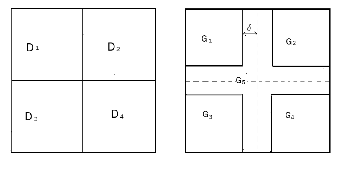
As in Figure 3, we first divide the domain $\Omega$ into four disjoint subdomains $D_{1}$ , $\cdots$ , $D_{4}$ such that $\bigcup_{j=1}^{4}\bar{D}_{j}=\bar{\Omega}$ , $D_{i}\cap D_{j}=\emptyset$ , then enlarge each $D_{j}$ to obtain $\Omega_{j}$ such that $G_{j}\subset\subset D_{j}\subset\Omega_{j}\subset\Omega$ for $i,j=1,2,3,4$ and

G_{5}=\Omega\setminus(\cup_{j=1}^{4}\bar{G_{j}}).

The sequence of finite element spaces is constructed by using the linear or quadratic element on the nested sequence of triangulations which are produced by the regular refinement with $\beta=2$ (connecting the midpoints of each edge).

Algorithm 4.2 is applied to solve the eigenvalue problem. If the linear element is used, from Theorem 4.2, we have the following error estimates for eigenpair approximation

\displaystyle|\lambda_{h_{n}}-\lambda|\lesssim h_{n}^{2},\ \ \|u_{h_{n}}-u\|_{1,\Omega}\lesssim h_{n}

which means the multilevel correction method can also obtain the optimal convergence order.

The numerical results for the first five eigenvalues and the $1$ -st, $4$ -th eigenfunctions (they are simple) by the linear finite element method with five levels grids are shown in Tables 1 and 2. It is observed from Tables 1 and 2 that the numerical results confirm the efficiency of the proposed algorithm.

Table 1: The errors for the first

5

eigenvalue approximations

Eigenvalues	$\|\lambda-\lambda_{h_{1}}\|$	$\|\lambda-\lambda_{h_{2}}\|$	$\|\lambda-\lambda_{h_{3}}\|$	$\|\lambda-\lambda_{h_{4}}\|$	$\|\lambda-\lambda_{h_{5}}\|$
1-st	0.073555	0.018534	0.004651	0.001164	0.000291
Order	–	1.988649	1.994561	1.998450	2.000000
2-nd	0.426525	0.106936	0.026747	0.006689	0.001673
Order	–	1.995883	1.999299	1.999515	1.999353
3-rd	0.426534	0.106939	0.026748	0.006689	0.001673
Order	–	1.995873	1.999285	1.999569	1.999353
4-th	1.078632	0.267624	0.066859	0.016717	0.004180
Order	–	2.010923	2.001014	1.999806	1.999741
5-th	1.490468	0.385000	0.097106	0.024349	0.006093
Order	–	1.952835	1.987226	1.995698	1.998638

Table 2: The errors for the simple (

1

-st and

5

-th) eigenfunction approximations

Eigenfunctions	$\\|u-u_{h_{1}}\\|_{1,\Omega}$	$\\|u-u_{h_{2}}\\|_{1,\Omega}$	$\\|u-u_{h_{3}}\\|_{1,\Omega}$	$\\|u-u_{h_{4}}\\|_{1,\Omega}$	$\\|u-u_{h_{5}}\\|_{1,\Omega}$
1-st	0.269991	0.135956	0.068195	0.034119	0.017064
Order	–	0.989771	0.995402	0.999091	0.999619
4-th	1.025704	0.514925	0.259424	0.129254	0.064645
Order	–	0.994180	0.989050	1.005103	0.999598

Next we discuss the effectiveness of $\delta$ and the coarsest mesh size $H$ to the numerical results by Algorithm 4.2. Figure 4 shows the errors for the different choices of $\delta$ and $H$ by the linear finite element method. From Figure 4, we can find Algorithm 4.2 can obtain the optimal convergence order when $H\leq 0.25$ and $\delta\geq 0.1$ which are soft requirements.

The case becomes better when we use the quadratic finite element method (see Figure 5). For the quadratic finite element, the convergence order ( $4$ -th) is always optimal even when $\delta$ is very small.

Example 6.2.

In the second example, we solve the eigenvalue problem (3.1) using linear and quadratic element on the square $\Omega=(-1,1)\times(-1,1)$ with $a(u,v)=\int_{\Omega}A\nabla u\cdot\nabla v\mathrm{d}\Omega$ , $b(u,v)=\int_{\Omega}\phi uv\mathrm{d}\Omega$ and

A=\begin{pmatrix}e^{1+x^{2}}&e^{xy}\\ e^{xy}&e^{1+y^{2}}\end{pmatrix}\ \ \text{ and }\ \ \phi=(1+x^{2})(1+y^{2}).

Since the exact eigenvalue is not known, we use the accurate enough approximations $[17.982932,33.384973,38.381968,47.670103,66.874113,68.323961]$ by the extrapolation method as the first $6$ exact eigenvalues to investigate the errors.

Figure 6 shows the corresponding numerical results for the first $6$ eigenvalues by the linear and quadratic finite element methods, respectively. Here, we use four level grids to do the numerical experiments. From Figure 6, the numerical results also confirm the efficiency of the proposed algorithm in this paper.

7 Concluding remarks

In this paper, we give a new type of multilevel local and parallel method based on multigrid discretization to solve the eigenvalue problems. The idea here is to use the multilevel correction method to transform the solution of eigenvalue problem to a series of solutions of the corresponding boundary value problems with the local and parallel method. As stated in the numerical examples, Algorithm 4.2 for simple eigenvalue cases can be extended to the corresponding version for multiple eigenvalue cases. For more information, please refer [18].

Furthermore, the framework here can also be coupled with the adaptive refinement technique. The ideas can be extended to other types of linear and nonlinear eigenvalue problems. These will be investigated in our future work.

References

[1] R. A. Adams, Sobolev spaces, Academic Press, New York, 1975.
[2] I. Babuška and J. E. Osborn, Finite element-Galerkin approximation of the eigenvalues and eigenvectors of selfadjoint problems, Math. Comp., 52 (1989), 275-297.
[3] I. Babuška and J. Osborn, Eigenvalue Problems, In Handbook of Numerical Analysis, Vol. II, (Eds. P. G. Lions and Ciarlet P.G.), Finite Element Methods (Part 1), North-Holland, Amsterdam, 641-787, 1991.
[4] J. H. Bramble, Multigrid Methods, Pitman Research Notes in Mathematics, V. 294, John Wiley and Sons, 1993.
[5] J. H. Bramble and X. Zhang, The analysis of Multigrid Methods, Handbook of Numerical Analysis, Vol. VII, P. G. Ciarlet and J. L. Lions, eds., Elsevier Science, 173-415, 2000.
[6] S. Brenner and L. Scott, The Mathematical Theory of Finite Element Methods, New York: Springer-Verlag, 1994.
[7] F. Chatelin, Spectral Approximation of Linear Operators, Academic Press Inc, New York, 1983.
[8] P. G. Ciarlet and J. L. Lions, Handbook of numerical analysis, Vol. II, finite element methods (Part I). North-Holland, 1991.
[9] X. Dai, L. Shen and A. Zhou, A local computational scheme for higher order finite element eigenvalue approximations, Int. J Numer. Anal. Model., 5 (2008), 570-589.
[10] W. Hackbush, Multi-grid Methods and Applications, Springer-Verlag, Berlin, 1985.
[11] P. Grisvard, Elliptic problems in nonsmooth domains, Pitman, Boston, MA, 1985.
[12] Q. Lin and H. Xie, A multi-level correction scheme for eigenvalue problems, http://arxiv.org/abs/1107.0223, to apper in Math. Comp., 2010.
[13] Q. Lin and H. Xie, A Type of Multigrid Method for Eigenvalue Problem, Research Report in ICMSEC, 2011-06 (2011).
[14] Q. Lin, H. Xie, and J. Xu, Lower bounds of the discretization for piecewise polynomials, Math. Comp., 83 (2014), 1-13.
[15] S. F. McCormick, ed., Multigrid Methods. SIAM Frontiers in Applied Matmematics 3. Society for Industrial and Applied Mathematics, Philadelphia, 1987.
[16] A. H. Schatz and L. B. Wahlbin, Interior maximum-norm estimates for finite element methods, Part II, Math. Comp., 64 (1995), 907-928.
[17] L. B. Wahlbin, Local behavior in finite element methods, in: Handbook of Numerical Analysis, Vol. II, Finite Element Methods (Part 1) (P. G. Ciarlet and J. L. Lions, eds.), 1991, 355-522.
[18] H. Xie, A Type of Multi-level Correction Method for Eigenvalue Problems by Nonconforming Finite Element Methods, Research Report in ICMSEC. 2012-10 (2012).
[19] J. Xu, Iterative methods by space decomposition and subspace correction, SIAM Review, 34(4) (1992), 581-613.
[20] J. Xu, A new class of iterative methods for nonselfadjoint or indefinite problems, SIAM J. Numer. Anal., 29 (1992), 303-319.
[21] J. Xu, A novel two-grid method for semilinear elliptic equations, SIAM J. Sci. Comput., 15 (1994), 231-237.
[22] J. Xu and A. Zhou, Local and parallel finite element algorithms based on two-grid discretizations, Math. Comput., 69(231) (1999), 881-909.
[23] J. Xu and A. Zhou, A two-grid discretization scheme for eigenvalue problems, Math. Comput., 70(233) (2001), 17-25.
[24] J. Xu and A. Zhou, Local and parallel finite element algorithm for eigenvalue problems, Acta Math. Appl. Sin. Engl. Ser., 18(2) (2002), 185-200.

	$\displaystyle\\|(I-P_{h})L^{-1}f\\|_{1,\Omega}$	$\displaystyle\lesssim$	$\displaystyle\rho_{\Omega}(h)\\|f\\|_{0,\Omega},\ \ \ \forall f\in L^{2}(\Omega),$
	$\displaystyle\\|u-P_{h}u\\|_{0,\Omega}$	$\displaystyle\lesssim$	$\displaystyle\rho_{\Omega}(h)\\|u-P_{h}u\\|_{1,\Omega},\ \ \ \forall u\in H_{0}^{1}(\Omega).$

	$\displaystyle\\|\widetilde{u}_{h_{k+1}}^{m+1}-P_{h_{k+1}}u\\|_{1/2,\partial G_{m+1}}^{2}$	$\displaystyle\lesssim$	$\displaystyle\sum_{j=1}^{m}\\|\widetilde{u}_{h_{k+1}}^{j}-P_{h_{k+1}}u\\|_{1/2,\partial G_{j}}^{2}$
		$\displaystyle\lesssim$	$\displaystyle\sum_{j=1}^{m}\\|\widetilde{u}_{h_{k+1}}^{j}-P_{h_{k+1}}u\\|_{1,G_{j}}^{2}$

			$\displaystyle\\|\widetilde{u}_{h_{k+1}}-P_{h_{k+1}}u\\|_{1,\Omega}^{2}$
		$\displaystyle\lesssim$	$\displaystyle\sum_{j=1}^{m}\rho_{\Omega_{j}}(H)^{2}\\|u_{h_{k}}-P_{h_{k+1}}u\\|_{1,\Omega_{j}}+\sum_{j=1}^{m}\\|{u}_{h_{k}}-P_{h_{k+1}}u\\|_{0,\Omega_{j}}^{2}$
			$\displaystyle\ \ \ +\sum_{j=1}^{m}\\|\lambda_{h_{k}}u_{h_{k}}-\lambda u\\|_{0,\Omega_{j}}^{2}+\\|\lambda_{h_{k}}u_{h_{k}}-\lambda u\\|_{0,G_{m+1}}^{2}$
		$\displaystyle\lesssim$	$\displaystyle\rho^{2}_{\Omega}(H)\\|{u}_{h_{k}}-P_{h_{k+1}}u\\|_{1,\Omega}^{2}+\\|{u}_{h_{k}}-P_{h_{k+1}}u\\|_{0,\Omega}^{2}+\\|\lambda_{h_{k}}u_{h_{k}}-\lambda u\\|_{0,\Omega}^{2}$
		$\displaystyle\lesssim$	$\displaystyle\rho^{2}_{\Omega}(H)\\|{u}_{h_{k}}-u\\|_{1,\Omega}^{2}+\rho^{2}_{\Omega}(H)\\|u-P_{h_{k+1}}u\\|_{1,\Omega}^{2}+\\|{u}_{h_{k}}-u\\|_{0,\Omega}^{2}$
			$\displaystyle+\\|u-P_{h_{k+1}}u\\|_{0,\Omega}^{2}+\|\lambda-\lambda_{h_{k}}\|^{2}\\|u\\|_{0,\Omega}^{2}+\lambda^{2}\\|u_{h_{k}}-u\\|_{0,\Omega}^{2}.$