Goodness-of-fit for log-linear network models: Dynamic Markov bases using hypergraphs
Abstract
Social networks and other large sparse data sets pose significant challenges for statistical inference, as many standard statistical methods for testing model/data fit are not applicable in such settings. Algebraic statistics offers a theoretically justified approach to goodness-of-fit testing that relies on the theory of Markov bases and is intimately connected with the geometry of the model as described by its fibers.
Most current practices require the computation of the entire basis, which is infeasible in many practical settings. We present a dynamic approach to explore the fiber of a model, which bypasses this issue, and is based on the combinatorics of hypergraphs arising from the toric algebra structure of log-linear models.
We demonstrate the approach on the Holland-Leinhardt model for random directed graphs that allows for reciprocated edges.
1 Introduction
Network data often arise as a single sparse observation of relationships among units, for example, individuals in a network of friendships, or species in a food web. Such a network can be naturally represented as a contingency table whose entries indicate the presence and type of a relationship, and whose dimension depends on the complexity of the model. This representation makes networks amenable to analysis by standard categorical data analysis tools and, in particular, it brings to bear the log-linear models literature, e.g. [BFH75]. However, given that often only a small sample or even just a single observation of the network is all we have access to, or that the data are sparse, several problems remain. In particular, in the case of network models, since quantitative methods are lacking, goodness-of-fit testing is usually carried out qualitatively using model diagnostics. Namely, the clustering coefficient, triangle count, or another network characteristic is used for a heuristic comparison between observed and simulated data. In [HGH08], the authors offer a systematic approach for comparing structural statistics between an observed network and networks simulated from the fitted model, and point out some of the difficulties of fitting the ERGMs. More recently, [GZFA09] review various network models and discuss modeling and fitting challenges that remain.
Even for linear exponential families, the problem of determining goodness of fit is a difficult one for network data. When standard asymptotic methods, such as approximations, are deemed unreliable (see [Hab81]), or when the observed data are sparse, one may want to use exact conditional tests. In such tests, the observed network (or table) with sufficient statistics vector is compared to the reference set, called the fiber , defined to be the space of all realizations of the network under the given set of constraints . Unfortunately, the size and combinatorial complexity of the fiber are the main obstacle for complete fiber enumeration, so that even in small problems (e.g., see [SZP, §4]), determining the exact distribution is often unfeasible. Moreover, fiber enumeration and sampling is crucial not only for goodness-of-fit testing but also for data privacy considerations (see [Sla]).
The theory of Markov bases provides a possible solution to the problem of sampling the fibers for any log-linear model. Namely, a Markov basis is a set of “moves” that, starting from any point in a fiber, allows one to perform a random walk on the fiber and visit every point with positive probability. Therefore, the standard Metropolis-Hastings algorithm provides a way to carry out exact tests, and as argued in [DS98], this procedure yields bona fide tests for goodness of fit. Furthermore, every log-linear model comes equipped with a non-unique but finite Markov basis. The existence and finiteness of the basis is a consequence of what is now often called the Fundamental Theorem of Markov Bases [DS98] in the algebraic statistics literature. However, two main computational challenges remain open to make this theory useful for network and large table data in practice. We describe these challenges broadly next and, then, address them in the remainder of this manuscript.
The first computational challenge is in determining the Markov basis itself. The fact that a Markov basis for a model guarantees to connect every one of its fibers makes it a highly desirable object to obtain. Unfortunately, the fastest algorithms for computing the moves for an arbitrary model (these algorithms exploit the toric structure of the model) are not fast enough. Even for some basic log-linear network models, it can take hours to find all Markov moves for networks with less than 10 nodes. This motivates a structural study of Markov bases for a given fixed family of models. To this end, the literature provides many examples [AT03, AT05], [DS03], [Dob03], [DS04], [HAT10], [HTY09b, HTY09a], [HMdCTY13], [KNP10], [Nor12], [RY10], [SW12], [YOT13]. In addition, since our example of interest is a network model with inherent sampling constraints, we should note that such constraints can compound the issue of computing a set of moves guaranteed to connect each fiber. Sampling constraints restrict the fiber, and in fact, if one is interested in sampling a restricted fiber, [OHT13] and [AHT12] show that one needs a larger set of moves, for example a Graver basis, to guarantee connectivity. A Graver basis (see [DSS09, §1.3], [AHT12, §4.6] for definition and discussion) is a particular Markov basis and generally contains more moves than a minimal Markov basis (where minimal is defined with respect to set inclusion).
The second computational challenge comes from the fact that knowing an entire Markov basis for a model may still not be sufficient to run goodness-of-fit tests efficiently. Namely, Markov bases are data-independent; see Problem 5.5. in [DFR+08]. To paraphrase [AHT12]: since a Markov basis is common for every fiber (that is, for all values that the vector of sufficient statistics can take), the set of moves connecting the particular fiber of the observed data will usually be significantly smaller than the entire basis for the model. To handle this issue Dobra, in [Dob12], suggests generating only moves needed to complete one step of the random walk, that is, only applicable moves. Dobra refers to the set of moves generated in this way as a dynamic Markov basis, since the full basis is not generated ahead of time. An example of this strategy is [OHT13], where the authors present an algorithm for generating a random element of the Graver basis for the beta model. The beta model is a basic generalization of the Erdös-Renyi random graph model: an ERGM for simple undirected random graphs where the degrees of the nodes form the sufficient statistics. In fact, this work can be cast within a more general framework of sampling from the space of contingency tables with fixed properties. A commonly fixed set of table properties are marginals of the table: they represent sufficient statistics of many - but not all - log-linear models. The paper [Dob12] focuses on log-linear models whose sufficient statistics are fixed marginals. There, the Markov moves are obtained through a sequential adjustment of cell bounds, a method that appears in sequential importance sampling (SIS) [CDS05], [DC11]. In contrast, we build a dynamic Markov basis by exploiting the combinatorics of the model. This allows us to extend Dobra’s methodology to log-linear models whose sufficient statistics are not necessarily table marginals.
In this manuscript, we explore the problem of performing goodness-of-fit tests for log-linear models when sufficient statistics are not necessarily table marginals, and in the presence of sampling constraints. In this case, there is no general methodology for obtaining the part of the Markov bases which is relevant for the observed data. In this work, we address the issues raised above from the point of view of algebraic statistics and combinatorial commutative algebra. We propose the use of parameter hypergraphs to generate Graver moves that are data-dependent and therefore applicable to the observed network (or table). Using Graver bases ensures connectivity of restricted fibers, while respecting sampling constraints. Furthermore, as [PS14] frame the Graver basis determination problem in terms of combinatorics of hypergraphs, we add this combinatorial ingredient to the recipe which allows us to generate the moves in a dynamic fashion, based on the observed table or network. The sufficient statistics for the model need not be table marginals; the only assumption we impose, mostly for simplicity, is that the model parametrization is squarefree in the parameters (see Section 2 for details). The random walk associated to the moves we produce in this way is irreducible, symmetric, and aperiodic, and so we may use the Metropolis-Hastings algorithm (see [RC99, §7]) to implement a Markov chain whose stationary distribution is equal to the conditional distribution on the fiber. This allows us to sample from the the fiber of an observed network or table as desired.
We illustrate our methodology and apply dynamically generated Markov bases to Holland and Leinhardt’s model [HL81]; specifically because previous methods are not applicable to this model directly. Holland and Leinhardt proposed to model a random directed graph by parametrizing propensity of nodes to send and receive links as well as reciprocate edges, where dyads are independent of each other. [PRF10, FPR10] study the algebra and geometry of these models and derive structural results for their Markov bases. Remarkably, the moves can be obtained by a direct computation only for networks with less than nodes, using 4ti2 [tt], currently the fastest software capable of producing such bases. Thus testing model fit for larger networks is not feasible using the traditional Metropolis-Hastings algorithm. Using a straightforward implementation of Algorithm 2 in R [Tea05], we test several familiar network data sets. Figure 1(a) shows the histogram of the values of the chi-square statistics for steps in the chain, including burn-in steps), obtained from Sampson’s monastery study [Sam68]. The vertical line denotes the value of the chi-square statistic for the observed monk dataset, indicating a large -value of and thus a pretty good model fit. A similar histogram in Figure 1(b) shows that the model does not fit the Chesapeake Bay food web data so well: the estimated -value is after moves.
This paper is organized as follows. Section 2 develops the combinatorial approach to the construction of Markov bases dynamically, and provides the necessary mathematical background. Section 3 illustrates the developed methodology for the Holland and Leinhardt’s model. Examples and simulations are in Section 4. Specifically, further discussion and analyses of the model fit for the directed networks arising from the monk and food web data can be found in Sections 4.4 and 4.5. Sections 4.3 and 4.2 provide studies of mobile money networks of a Kenyan family, and of four networks simulated from the distribution, respectively. Finally, simulations on a small synthetic network in 4.1 indicate good mixing times, and quick convergence of the -value estimate (e.g., see Figure 7(b)). As this is best illustrated when the entire fiber has been determined exactly, we also consider a small -network fiber for an undirected graph on nodes from Section 5.1. in [OHT13]. Our walk explores the entire fiber in as little as moves and the total variation distance from the uniform distribution is below 0.25 after moves. This could be due to the fact that the steps in the simulated walks are longer than minimal Markov moves would suggest, since we are generating a superset of the Graver basis in our algorithm.
2 Parameter hypergraph of a log-linear model: revised Metropolis-Hastings
Markov and Graver bases arise as combinatorial signatures of log-linear models, and this natural correspondence is rooted in the algebra-geometry dictionary. In this section, we briefly describe the mathematical construction that allows us to dynamically generate applicable moves for sampling fibers of general log-linear models.
2.1 Markov bases: fundamentals
Consider a log-linear model on a contingency table with sufficient statistics vector . Let be a realization of the table , with . The fiber of , which we will denote (or simply if the observed table is implied from the context), is the space of all realizations of the table whose sufficient statistics are the same as that of ; i.e., . For two tables in the same fiber , the entrywise difference is called the move from table to table . This move is another -way table with entries equal to zero in the cell if , a positive integer in the cell if , and a negative integer in the -cell otherwise. Note that, by definition, is linear, thus the sufficient statistic of any move connecting two tables in the same fiber, , is zero. In particular, adding a move to a contingency table does not change the values of the sufficient statistics vector. We will call any table such that a Markov move on . Thus, to discuss walks on a fiber, we may either specify the start and target tables and , or the Markov move .
A Markov basis is a set of Markov moves such that for any fiber and any two contingency tables , there exists a sequence of moves such that is reachable from by the corresponding walk on the fiber , i.e., and each partial sum , , is a table in the fiber (that is, has nonnegative entries). The existence and finiteness of a Markov basis guaranteed by the fundamental theorem of Markov bases [DS98], which states that the moves correspond to generators of an algebraic object (namely, the toric ideal) associated with each log-linear model. Equipped with a set of moves, one can perform a random walk on the fiber . A priori, the resulting Markov chain need not be irreducible; however, if the set of moves is a Markov basis, then irreducibility is guaranteed. Moreover, a Metropolis-Hastings algorithm can be used to adjust the transition probabilities, returning a chain whose stationary distribution is exactly the conditional distribution on the given fiber.
In this section, we discuss how to dynamically construct arbitrary elements of a Markov basis for any log-linear model using the parameter hypergraph of the model. For simplicity, we restrict ourselves to log-linear models with design matrices (that is, parameters do not appear with multiplicities in the model parametrization), although the definition and construction could be extended to a more general case. As mentioned in the introduction, this will be specifically useful in several cases: when cannot be computed in its entirety, e.g. when the model is not decomposable, so that the divide-and-conquer strategy of [DS04] cannot be applied, and when sufficient statistics of the model are more complex than table marginals. To that end, we define the main tool of our construction.
2.2 From tables to hypergraphs
Let be any log-linear model for discrete random variables with sufficient statistics . Suppose that the joint probabilities of the model are such that the parameters appear without multiplicities (that is, can be obtained from the table in a linear fashion).
Definition 2.1.
The model is encoded by a hypergraph on the vertex set , which is constructed as follows: is an edge of if and only if the index set describes one of the joint probabilities in the model; that is, there exist values such that, up to the normalizing constant, . The hypergraph is called the parameter hypergraph of the model .
Notation 1.
For convenience let us gather here the notational conventions we will use throughout. Log-linear models will be denoted by with sufficient statistics , or simply when clear from context. The parameter hypergraph has vertex set and edge set . Edges in the hypergraph are written as products of parameters instead of the usual lists, e.g., will represent the edge .
The easiest way to understand is by viewing it as depicting the structure of parameter interactions. Since vertices of the hypergraph represent parameters of the model, edges in collect all the parameters that appear in a joint probability under the model. There is a one-to-one map between the contingency table cell labels and edges in the parameter hypergraph. Let us illustrate on two simple but familiar examples.
Example 2.2 (Two independent random variables).
Consider the model of independence of two discrete random variables and , taking and values, respectively. Denote the marginal probabilities and by and , respectively. Since the independence model for and is specified by the formula , we see that the parameter hypergraph has vertices: and an edge between every and . Thus, in this case, the hypergraph is just a complete bipartite graph on , depicted in Figure 2(a).
Example 2.3 (Quasi complete independence).
For a table, the quasi complete independence model is a complete independence model with structural zeros. If the cell is a structural zero, then , otherwise where , , and are marginal probabilities.
To obtain the parameter hypergraph for the quasi complete independence model, we start with the complete 3-partite hypergraph with vertex partition , , and such that , , and , then remove every edge that corresponds to a cell with a structural zero. The hypergraph in Figure 2(b) is the parameter hypergraph for the quasi complete independence model on a table where all cells are structural zeros except , and .

In the next section (Definition 3.1) we will see a more complex example in , the parameter hypergraph for the version of the model that assumes edge-dependent reciprocation.
A crucial observation about the parameter hypergraph is that it not only encodes the parameter interactions, but any observed table can be viewed as a subset of its edges, with multiplicities if the model allows them. Specifically, suppose the table has an entry in the cell . If the model postulates , then the -cell entry is represented by the edge . A larger entry (say, ) in the table would be represented by an edge with multiplicities (the edge would have multiplicity ). Multiplicities are recorded with a function (e.g. .
Definition 2.4.
The list of edges
will be denoted by . It is the multiset of edges representing the table , and has support in the edge set of the parameter hypergraph.
Next, notice that sufficient statistics can be calculated from the hypergraph edges , since the vertices covered by represent those natural parameters that affect the computation of . In the independence model example (cf. Example 2.2), if is the table with in cell and a in the cell , then . The sufficient statistics of the table under are the row and column sums; the first row having sum means that appears once in the set of edges ; in other words, the degree of the vertex is . The first column having sum means that has degree in . Therefore, the vector of sufficient statistics equals the degree vector of the multi-hypergraph . It is obtained by simply counting the number of edges incident to each vertex in and setting the degree of all other vertices in to zero.
Finally, we describe how to construct and explore the fiber . Preserving the value of the vector means finding another edge set such that the degree vector of is the same as that of . If we view the edges as colored red and blue, then the move corresponds to a collection of edges , where each vertex appears in the same number of blue and red edges.
We have thus shown the following is an equivalent way to view the fiber and its connecting moves.
Theorem 2.5.
Recall that an observed table is represented by a multiset of edges on the hypergraph .
- (a)
The fiber consists of all multisets of edges of with degree vector equal to .
- (b)
Any move in the Markov basis connecting to some is represented by the edge sets over the parameter hypergraph such that the degree vector of is the same as that of .
We call such a collection a (color-)balanced edge set; it was defined and discussed in more detail in [PS14], where it was shown that such sets constitute a Markov (and in fact, the Graver) basis for any parameter hypergraph. Complexity of minimal Markov moves to connect the given (unrestricted) fiber was studied in [GP13]. For convenience, let us summarize here the hypergraph notation we will use in the following section.
Notation 2.
For an observed table , the set of red (observed) hyperedges will be denoted by , and any blue set that balances the vertices covered by will be denoted by . Note that every corresponds to a table . The move will be denoted as .
Remark 2.6.
By abuse of notation, we will also denote by only those edges over representing the non-zero entries of the move . Indeed, if a cell has the same value in both tables, the move directly connecting the tables does not affect that cell, thus the corresponding edge need not be recorded in . If it is included in this set, then the move simply subtracts and adds to the cell in the table, that is, it removes and then adds back the particular edge in .
2.3 Sampling constraints and restricted fibers
As mentioned briefly in the introduction, a Markov basis will connect all table realizations in a fiber that are subject to the constraint that each table entry is non-negative. However, in the presence of table cell bounds or structural zeros in the model (e.g. [BFH75, §5.1]), Markov moves will inevitably produce tables whose cell entries are too large, even if they satisfy the sufficient statistics (say, the realization of the table reached by the random walk will have the given marginals, but some cells will be out of bounds). These sampling constraints often arise in real-world data. In the network modeling case, a structural zero means a certain relation or edge can never be observed, while a cell bound puts a restriction on how many times an edge between two nodes can be observed in any instance of the network. In fact, most (simple) network models begin with a basic assumption that allows only one edge per dyad, for example, the model [HL81] (see also [FPR10]) and the beta model [CDS11]. This clearly introduces another problem for running random walks on fibers: at any given step, the table or network produced may not be observable, and so many of the steps in the walk will be rejected. In fact, the rejection is likely to occur because the usual Markov bases are blind to data and sampling constraints. To compound this problem, a Markov basis only guarantees that the fiber of non-negative table realizations is connected. It is quite reasonable to expect that there exist two of them that can be connected only by a walk that passes through another table realization which does not satisfy the additional cell bounds. In this sense, the sampling constraints have suddenly disconnected the fiber ! With this in mind, we will differentiate between the usual fiber and what we call the observable fiber :
Definition 2.7.
The observable fiber is the set of all realizations of the contingency table with nonnegative entries and sufficient statistic that respect the sampling constraints of the model, i.e. integer bounds on cells or structural zeros.
For example, in the model, the observable fiber contains only simple directed graphs, which means each cell in the contingency table representing the directed graph is either a or a . Naturally, there is a corresponding condition on the hypergraph: no edge in representing the table can have multiplicity larger than . Thus any move applied to must be such that in the resulting set of edges, , every edge appears at most once.
Thus, a natural question arises: does there exist a finite set of moves that connects the observable fiber? The answer is known in the literature under the name of Graver basis or distance-reducing moves. Hara and Takemura study the observable fibers for contingency tables, that is, tables with cell bound of everywhere, and show [HT10, Proposition 2.1] that the squarefree part of the Graver basis will connect any fiber respecting sampling constraints. Here, “squarefree part” simply means that each entry in the table representing the move is either or ; we will say that such a move respects the sampling constraint. Their result is, in fact, more general, and applies to higher integer cell bounds and structural zeros as well:
Proposition 2.8 ([HT10]).
The elements of the Graver basis which respect the sampling constraints suffice to connect the observable fiber in all cases where sampling constraints are integer bounds on cells.
The proof relies on an algebraic fact that moves correspond to binomials in a toric ideal, and every binomial arising from the given model can be written as what is called a conformal sum of Graver basis elements. We will not go into technical details of this result here; the reader is referred to [Stu96] and recent text [AHT12].
2.4 Applicable moves and revised Metropolis-Hastings
In general, the set of squarefree moves from the Graver basis is much larger than a minimal Markov basis. In particular, this set almost never equals the squarefree moves from a minimal basis. Moreover, it is notoriously difficult to compute, providing another reason against pre-computing the moves for the given model, and instead, generating dynamically only those moves that can be applied to the observed table or network and remain in the observable fiber .
Definition 2.9.
A move is said to be applicable to a point in the fiber (equivalently, to the network represented by a table ) if it produces another point in the observable fiber , respecting the sampling constraints of the model at hand.
In terms of the hypergraph edges, the move , represented as , is applicable if for some table .
We can thus extend Theorem 2.5 to characterize applicable Graver moves in terms of the parameter hypergraph: By Theorem 2.8 in [PS14] and the Fundamental Theorem of Markov bases, any move corresponds to a balanced edge set of . Furthermore, moves in the Graver bases correspond to the primitive balanced edge sets of . We can summarize applicable Graver moves in terms of in the following way.
Corollary 2.10.
Adopt Notation 2. Any move in the Graver basis that is applicable to is a set of edges such that:
- 1.
,
- 2.
for some table , and
- 3.
there exists no move such that and .
In the result above, 1. ensures non-negativity of the resulting table , 2. ensures the move is applicable, and 3. ensures the move is a Graver basis element. In practice, however, checking 3. is a non-trivial task; instead, an algorithm with positive probability for producing each Graver move suffices for goodness of fit testing purposes. Thus, in Section 3 we run walks on fibers using elements of the Graver basis along with some larger applicable moves as well.
The remainder of this section discusses how to construct applicable moves and embeds the combinatorial idea from Corollary 2.10 within the Metropolis-Hastings algorithm to perform random walks on fibers.
If the procedure for finding in step 4 is symmetric and non-periodic, then Algorithm 1 is a Metropolis-Hastings algorithm and as the output will converge to ([DSS09], [RC99]). Ideally, Step 4 should take advantage of the specific structure of the hypergraph. For example, we employ this process to implement Algorithm 1 and produce applicable moves on the fly for the Holland-Leinhardt model in Section 3.
The use of allows us to bypass two crucial issues of the usual chain, as stated in [DS98], which relies on precomputing a minimal Markov basis, and which are summarized in the last paragraph of [Dob12]. First, Algorithm 1 does not require computing the full Markov basis, or the full Graver basis as may be required due to sampling constraints. Second, the rejection step from the usual Metropolis-Hastings is bypassed, since rejections are due to the fact that most moves drawn from the full Markov basis will be non-applicable to the current table. This, in turn, should have positive impact to the mixing time of the chain.
Example 2.11.
Suppose we observe a contingency table all of whose entries are except the and entries, which are . There are 200 moves in a minimal Markov basis for the independence model . However, only one of those is applicable: namely
or, written in terms of the parameter hypergraph, where and . This move replaces the entries and by , and entries and by . Any other move will produce negative entries in the table and thus move outside the fiber. A more interesting example can be similarly constructed on a -way table that is either sparse or has many non-zero entries but allows only entries.
Next, suppose the observed table is
The table is represented by the multiset of edges
from the independence model (hyper)graph illustrated in Figure 2(a). Denote the bipartite (hyper)graph in Figure 2(a) as . It is known that any Markov move for the independence model corresponds to a collection of closed even walks on , and any Graver move corresponds to a primitive closed even walk on . For a detailed account of the correspondence between primitive balanced edge sets of and primitive closed even walks see [Vil00]. Due to this correspondence, a natural procedure for performing Step 4 in Algorithm 1 is to randomly select a set of edges from , say, , and then complete a closed even walk on , so that the new edges form . Notice and have the same degree vector and is applicable to . This move is depicted in Figure 3. The first figure is the parameter hypergraph. The second represents the observed table , with edges in highlighted. The third is the edge set with highlighted. The resulting table is
3 Application to the -model
In a seminal 1981 paper [HL81], Holland and Leinhardt described what they referred to as the model for describing dyadic relational data in a social network summarized in the form of a directed graph. Their model, which is log-linear in form ([FW81]), allows for effects due to differential attraction (popularity) and expansiveness, as well as an additional effect due to reciprocation. For each dyad, a pair of nodes (, the parameter describes the effect of an outgoing edge from , and the effect of an incoming edge pointed towards , while corresponds to the added effect of reciprocated edges. The parameter quantifies the average “density” of the network, i.e. the tendency of having edges, and is a normalizing constant to ensure that the probabilities for each dyad add to 1.
Given a directed graph, each dyad can occur in one of the four possible configurations: no edge, edge from to , edge from to , and a pair of reciprocated edges between and . The model postulates that, for each pair , the probability of observing the four possible configurations, in that order, satisfy the following equations:
where
We will focus on the edge-dependent version of the reciprocation parameter, where .
Making the following substitutions
and ignoring the superscripts for convenience, we arrive at the following simplified equations to describe the probability of observing each configuration for a pair :
While normalizing constants are usually ignored, we will follow [PRF10] and treat as a model parameter. The advantage of this technique is that, given an observable network , these extra parameters ensure that the sampling constraint of a dyad (pair) being observed in one and only one state is satisfied for all networks in .
Definition 3.1 (The parameter hypergraph of the model).
We will denote the parameter hypergraph of the model as . Recall that the hyperedges of are determined by the parameters appearing in the joint probabilities of the model. Thus, for the model with edge reciprocation there are three types of hyperedges: singletons (corresponding to for each dyad ), hyperedges of size (corresponding to and ), and hyperedges of size (corresponding to ).
More formally, , where , and , with , , and .
3.1 Markov moves for the model
Here we describe the form of a Markov move for the model with edge-dependent reciprocation in terms of the parameter hypergraph given in Definition 3.1. The moves can be described in terms of balanced edge sets on a graph obtained by contracting hyperedges in . Note that by definition, balanced edge sets on graphs reduces to collections of closed even walks.
Let be the undirected bipartite graph on vertices with vertex set
and edge set
Let be the undirected complete graph on the vertices . The graphs and can be constructed from as follows. To construct from , simply consider all hyperedges of size in . Each of these hyperedges has vertices for some . The contracted edges (with deleted) are precisely the edges in . To construct , consider all hyperedges of size in . Note that each of these edges corresponds to an edge in that has vertices for some . Deleting all the vertices except from each hyperedge of size contracts them to size , and the result is the complete graph on the vertices .
Let be the subhypergraph of where and . The previous two paragraphs describe a bijection between the edge sets of and :
For a simple balanced edge set of , the set may not be balanced. However, it can become balanced by appending edges of the form to the sets and . Thus, we define a lifting operation that grows to a simple balanced edge set of in this manner:
Let be the subhypergraph of that contains all the hyperedges of of size 7. Let be the subhypergraph of that contains all the hyperedges of of size 3. If is a balanced edge set of then each in the hyperedges of size 7 of must be color-balanced. This implies that the ’s and ’s are color-balanced with respect to . Thus, it follows that the ’s and the ’s are color-balanced in . These observations are noted in [PRF10], but in algebraic terms using the binomials of the ideal of the hypergraph .
Since a balanced edge set on is a move between two observable networks only if , we arrive at the following proposition.
Proposition 3.2.
A move between two observable networks and in the same fiber is of the form lift such that is a balanced edge set on and .
Corollary 3.3.
For the model with edge-dependent reciprocation, the set of all such that and is a balanced edge set of and connects the observable fiber for every possible sufficient statistic .
Remark 3.4.
The set of moves described in Corollary 3.3 is a superset of the square-free Graver basis.
3.2 Generating an applicable move
Now that we have described the general form for the Markov moves for the model, we give an algorithm for generating an applicable move. Let be an observable network written as the union of its reciprocated part and its unreciprocated part . For a directed graph , let undir() be the edges of the skeleton of and let recip()=(, recip( where recip. The following is a general algorithm for generating applicable moves for the model with edge-dependent reciprocation. It uses the fact that every balanced edge set of a graph corresponds to a set of closed even walks on that graph. The output is either an element of the Graver basis, or an applicable combination of several Graver moves, which themselves need not be applicable. Since the hyperedges of a balanced edge set on each correspond to a dyadic configuration realizable in the network, we will return moves in the form where are the edges to be removed from the network and are the edges to be added.
Example 3.5.
Figure 4 illustrates the process of generating a Type 2 move. First the edges , , and from a network are chosen. These will be the edges that are removed from in the move. We consider these edges as edges of . A walk is completed on by adding the blue edges , and . The blue edges are then interpreted in terms of pairs and dyadic configurations in . These are the edges that are added to in the move.

Remark 3.6.
Notice that in each of the above algorithms, it is possible that the trivial move is returned. This means the walk in Algorithm 1 would stay in the same place at that step. While this does not affect the stationary distribution of the Markov chain, it can have a negative impact on mixing times if too many trivial moves are returned. However, this is the problem also with the usual Metropolis-Hastings algorithm, as mixing time questions are generally open. Section 4 shows some indication that the chain seems to be mixing well. In the case of the model, the probability of returning the trivial move in any of the above algorithms depends on the in and out-degree sequences of the unreciprocated edges and the reciprocated edges. One direction for further research is to understand and try and reduce the output of trivial moves. Even understanding which networks result in a high probability of a trivial move being returned in Algorithms 3, 4, 5, would be an interesting combinatorial problem.
Proposition 3.7.
Proof.
Algorithm 3 chooses a set of edges from undir and completes closed even walks on . We will denote the balance edge set of corresponding to this set of closed even walks as . Step 7 checks that lift satisfies . If the condition is not satisfied, then the trivial move is returned. Otherwise, outputted by Algorithm 3 is of the form of the specified. Applicability of follows from the fact that is a subset of and . Moves outputted from Algorithms 4, 5 can be analyzed in a parallel fashion.
For the second part of the statement, Proposition 3.2 states that the move between two networks , in the same fiber is of the form lift where is a balanced edge set on . Assume that is contained entirely in . Denote the closed even walks on that correspond to as . The move will be returned if is chosen in Algorithm 2, the edges of corresponding to are chosen at Step 1 of Algorithm 3, and Steps 3 and 4 result in a sequence such that corresponds to a cyclic permutation of the odd edges of . If is contained entirely in or contains edges from both and , then a similar argument follows. ∎
Theorem 3.8.
Let be an observable network with more than 2 edges and with sufficient statistic . The Markov chain, , where the step from to is given by Algorithm 2 is an irreducible, symmetric, and aperiodic random walk on .
Proof.
Irreducibility follows Proposition 3.7.
To show symmetry, let and be two simple networks with reciprocated parts , and unreciprocated parts , . The move from to is the combination of moves from to and from to where and . The move corresponds to a balanced edge set on , which forms a set of primitive closed even walks on . The probability of choosing in Step 1 of Algorithm 3 is dependent only on the number of edges in , which is equal to the number of edges in . Step 5 in Algorithm 3 completes walks on sequences of edges from by connecting heads to tails. Thus, given that was chosen in Step 1, the probability of choosing an ordering of the vertices, an ordering of the edges, and a composition in Steps 2-4 such that Step 5 will output is dependent only on the structure of (the primitive walks in , the length of these walks, and which of these walks share a vertex). So, since is the same regardless whether we are moving from to or from to , the probabilities of making these moves in a single step are equal. A similar situation occurs between the reciprocated parts of and .
For aperiodicity, notice that every non-diagonal entry of the transition matrix of is greater than zero. Therefore, since contains more than two edges, for all . ∎
Corollary 3.9.
If has more than two edges, then with probability one
Algorithm 2 and it’s subroutines Algorithms 3, 4, 5 are implemented in R; the code is available in the supplementary material on [GPS]. The examples in Section 4 that compute estimated -values use the function Estimate.p.Value. It takes an observed network and implements Algorithm 1 using an iterative proportional scaling algorithm [HL81, p.40] to compute the MLE, and Algorithm 2 for Step 4. We chose to use the chi-square statistic for the goodness-of-fit statistic.
Our implementation makes use of the R package igraph [CN06], and in particular its graph data structure and methods for producing graph unions and graph intersections. Each of these methods has complexity linear in the sum of the cardinalities of the edge sets and vertex sets of the input. As a result the complexity of the algorithm is at worst O, where V and E are the vertex and edge sets respectively.
4 Simulations
We apply Algorithms 1 and 2 and run goodness-of-fit tests in R on several real-world network datasets as well as simulated networks under the model. In what follows, reported are the number of steps in the chain along with the initial burn-in. Our statistic of choice for is the chi-square statistic, directly measuring the distance of the network from the MLE. For each simulation, we report the estimated -value returned on line 11 of Algorithm 2 and the sampling distribution of .
4.1 A small synthetic network
We begin with a test case to check how Algorithm 2 explores the fiber. In [OHT13, §5.1], the authors sample the fiber of an undirected graph on nodes, depicted in Figure 6, under the beta model. By enumeration they have determined that the size of the fiber is . Considering this graph as a directed network all of whose edges are reciprocated, we can test the fit of the model as well, and study its fiber similarly. The fibers of under the two models are the same, since in both cases, the fiber consists of all undirected (or reciprocated-edge) graphs with the same (in- and out-) degree vector as .
We ran Algorithm 2 and stored all graphs discovered in the run. Starting from , after steps, points in the fiber were discovered. After steps, graphs were discovered; and the entire fiber of graphs was reached after less than steps in the chain. At this point, the chain samples the fiber almost uniformly, as the total variation distance between the sampling distribution and the uniform distribution on the fiber is calculated to be (at the -th step). For comparison purposes, the TV-distance is after steps; Figure 6 shows the histogram of graphs sampled in the -move walk. Therefore, running a Markov chain of at least steps should be sufficient for testing purposes for this example.
A run of Algorithm 1 for steps, after burn-in steps, produced the values of the chi-square statistics in Figure 7(a), and the -value estimate of . The estimates of the p-value from the simulation are plotted in Figure 7(b) against the step number of the Markov chain and give further evidence of convergence.
4.2 Networks simulated from the distribution
Consider the four digraphs on nodes that Holland and Leinhardt simulated from the distribution; see [HL81, Figure 3]. The networks are depicted in Figure 8.
For each network, chains of length provide expected results. The estimated p-values are , , and , respectively. The histograms of the sampling distribution of the chi-square statistics from the -step simulation (with burn-in steps) are shown in Figure 9. The p-values reach their estimated value in approximately steps after burn in.
-value:
-value:
-value:
-value:
4.3 Mobile money networks
Figure 11 is a directed graph on 12 vertices with 13 unreciprocated edges and 15 reciprocated edges. The data is from [KCGK] and was collected through a survey conducted in Bungoma and Trans-Nzoia Counties in Kenya, and among Kenyans living in Chicago, Illinois in the summer of 2012. Vertices represent members of an extended family. An edge from vertex to vertex represents that had sent money to using a mobile money transfer. Since the network depicted in Figure 11 is a social network and the individuals are social actors, it is reasonable to suspect transitive effects are present. In such a setting, it is expected the model would not fit this data very well, and, Holland and Leinhardt suggest [HL81] the model as a realistic null model in such cases.
Running Algorithm 1 for 300,000 steps after an initial burn-in of 30,000 steps returns an estimated p-value of , which would suggest that the model with edge dependent reciprocation is indeed a poor fit for this data, and in fact, if the significance level is set to less than we would reject the model. Figure 11(a) shows the histogram of the sampling distribution of the chi-square statistics with the chi-square statistic for the observed network marked in red. Figure 11(b) shows the estimated p-value plotted against the step number of the Markov chain and gives evidence of convergence.
4.4 Chesapeake Bay Ecosystem
In their 1989 paper [BU89], Ulanowicz and Baird constructed trophic networks for specific regions of the Chesapeake Bay using extensive data gathered from 1983-1986. Their work used highly sophisticated estimation methods, relying on a multitude of different sources. Due to their profound detail, Ulanowicz and Baird’s food webs have been extensively analyzed over the last 25 years. Often for statistical model-fitting purposes, the edges are considered as undirected. This choice, however, has been largely motivated by the scarcity of tools available to analyze directed networks. Other than heuristic methods, procedures for performing goodness of fit testing for directed network models have not existed.
The data set on which we test the model is depicted in Figure 12; see also [BU89, Figure 2]. The list of edges of this directed network was downloaded from [Paja] and represents the Web 34 Chesapeake Bay Mesohaline Ecosystem. The graph has 39 vertices and 176 edges. The majority of vertices represent species in a Chesapeake Bay food web, with a directed edge indicating that species eats species . Although, we note there are also other elements, which are not species, included as vertices as well, such as passive carbon storage compartments. There are reciprocated edges in the graph.
We expect a block structure in food networks that do not naturally occur in -model generated networks. In fact, the estimated p-value is , indicating that the model with edge dependent reciprocation is not a good for this data. If the significance level is set to less than , we would reject this model. The histogram of a simulation with steps is shown in Figure 1(b).
4.5 Sampson’s Monastery Study
Sampson [Sam68] conducted an ethnographical study of social interactions between novices in a New England monastery in the mid 1960s. Sampson observed novices over a period of two years, gathering social relations data at 4 time points, and on multiple relationships. This has been a favorite example for analysis by sociologists, statisticians and others, and was used in original model studies. At the fourth time point (), there were monks, and the social network had 54 directed edges representing the top three answers to the question “whom do you like” for each novice. We consider the directed graph in Figure 13 representing the relationships derived from this affinity sociometric data. The list of edges in the graph was downloaded from [Pajb].
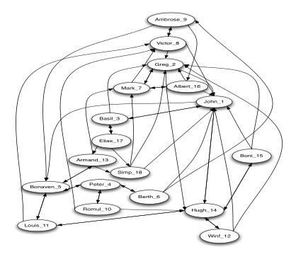
Perhaps not unsurprisingly, the -model with edge-dependent reciprocation seems to fit this data remarkably well. The chi-square statistic for the observed network is 404.7151, which is very close to the minimum chi-square statistic that was returned during a 1,000,000 step walk (see Figure 14(a)). The estimated -value for this data is . The random walk seems to be exploring the fiber broadly, discovering about new networks every steps, though we do not know the exact size of the fiber.
5 Conclusion
The central motivation for this work is the scarcity of tools available to analyze directed networks. Other than heuristic methods, procedures for performing goodness of fit testing for directed network models have not existed. In the usual setting, the Metropolis-Hastings algorithm for sampling from conditional distributions requires a Markov basis for a given model to be precomputed. By definition, however, Markov bases are data independent, thus presenting a computational problem that becomes both wasteful and infeasible for network models on as few as nodes. In addition, sampling constraints (e.g. one edge per dyad in a network or cell bounds in a contingency table) have presented problems for algebraic statistics as the restricted (observable) fibers cannot always be connected with a minimal set of Markov moves. Instead, a knowledge of a much larger set of moves, such as the Graver basis, is required for sampling. Since Graver bases are notoriously difficult to compute except for (notable) special cases (e.g. where a divide-and-conquer strategy applies, as in decomposable models), being able to dynamically generate one applicable move at a time is essentially the only hope for ever being able to utilize the algebraic statistics idea in practice.
Using the work by Dobra [Dob12] as our main motivation, we propose a methodology for dynamically generating moves and combinations of moves from the Graver basis (and thus a Markov basis) that guarantee to connect observable fibers for networks or contingency tables where sufficient statistics are not necessarily table marginals. This approach allows for a data-oriented algorithm, providing a dynamic exploration of any fiber without relying on an entire Markov basis. It produces only a relatively small subset of the moves - which could still be a large subset indeed - needed to connect the observable points in the fiber.
In contrast with previous approaches, our proposed modification uses moves that are constructed by understanding the balanced edge sets of the parameter hypergraph of the given model. Drawing upon the classical literature in combinatorial commutative algebra and recent work in algebraic statistics, we show how, in principle, one can construct applicable moves using the parameter hypergraph of any log-linear model and any observed network. Thus, in situations where the structure of the parameter hypergraph is well understood, this allows for easily implementable algorithms for goodness-of-fit testing. As an example, we describe the entire procedure on the model with edge-dependent reciprocation. For the model, we (1) derive the structure of such the Markov moves in relation to the parameter hypergraph and (2) implement an algorithm to generate them dynamically. We hope this technique of analyzing the parameter hypergraph to construct dynamic Markov bases will be used for other log-linear models and spurs new ideas for goodness-of-fit testing for exponential random graph models in general.
Acknowledgements
The authors are grateful to Alessandro Rinaldo and Stephen E. Fienberg for their support at the inception of this project. The first author is supported by the NSF Postdoctoral Research Fellowship, NSF award #DMS-1304167. The second and third authors acknowledge partial support from grant #FA9550-12-1-0392 from the U.S. Air Force Office of Scientific Research (AFOSR) and the Defense Advanced Research Projects Agency (DARPA). Some computations are performed on a cluster provided by an NSF-SCREMS grant to IIT.
References
- [AHT12] Satoshi Aoki, Hisayuki Hara, and Akimichi Takemura, Markov bases in algebraic statistics, Springer Series in Statistics, Springer New York, 2012.
- [AT03] Satoshi Aoki and Akimichi Takemura, Minimal basis for a connected Markov chain over contingency tables with fixed two-dimensional marginals, Australian & New Zealand Journal of Statistics 45 (2003), no. 2, 229–249.
- [AT05] , Markov chain Monte Carlo exact tests for incomplete two-way contingency tables, Journal of Statistical Computation and Simulation 75 (2005), no. 10, 787–812.
- [BFH75] Yvonne M. Bishop, Stephen E. Fienberg, and Paul W. Holland, Discrete multivariate analysis: Theory and practice, Springer, New York, 1975.
- [BU89] D. Baird and R.E. Ulanowicz, The seasonal dynamics of the Chesapeake Bay ecosystem., Ecol. Monogr. 59 (1989), 329–364.
- [CDS05] Yuguo Chen, Ian H. Dinwoodie, and Seth Sullivant, Sequential importance sampling for multiway tables, Annals of Statistics 34 (2005), 523–545.
- [CDS11] Sourav Chatterjee, Persi Diaconis, and Allan Sly, Random graphs with a given degree sequence, Ann. Appl. Probab. 21 (2011), no. 4, 1400–1435.
- [CN06] Gabor Csardi and Tamas Nepusz, The igraph software package for complex network research, InterJournal Complex Systems (2006), 1695.
- [DC11] Ian H. Dinwoodie and Yuguo Chen, Sampling large tables with constraints, Statistica Sinica 21 (2011), 1591–1609.
- [DFR+08] Adrian Dobra, Stephen E. Fienberg, Alessandro Rinaldo, Aleksandra Slavković, and Yi Zhou, Algebraic statistics and contingency table problems: Log-linear models, likelihood estimation and disclosure limitation, IMA Volumes in Mathematics and its Applications: Emerging Applications of Algebraic Geometry, Springer Science+Business Media, Inc, 2008, pp. 63–88.
- [Dob03] Adrian Dobra, Markov bases for decomposable graphical models, Bernoulli 9 (2003), no. 6, 1093–1108.
- [Dob12] , Dynamic Markov bases, Journal of Computational and Graphical Statistics (2012), 496–517.
- [DS98] Persi Diaconis and Bernd Sturmfels, Algebraic algorithms for sampling from conditional distribution, Annals of Statistics 26 (1998), no. 1, 363–397.
- [DS03] Mike Develin and Seth Sullivant, Markov bases of binary graph models, Annals of Combinatorics 7 (2003), no. 4, 441–466.
- [DS04] Adrian Dobra and Seth Sullivant, A divide-and-conquer algorithm for generating Markov bases of multi-way tables, Computational Statistics 19 (2004), 347–366.
- [DSS09] Mathias Drton, Bernd Sturmfels, and Seth Sullivant, Lectures on algebraic statistics, Oberwolfach Seminars, vol. 39, Springer, 2009.
- [FPR10] Stephen E. Fienberg, Sonja Petrović, and Alessandro Rinaldo, Algebraic statistics for random graph models: Markov bases and their uses, vol. Papers in Honor of Paul W. Holland, ch. 1, Springer, 2010.
- [FW81] Stephen E. Fienberg and S. S. Wasserman, Discussion of Holland, P. W. and Leinhardt, S. “an exponential family of probability distributions for directed graphs.”, Journal of the American Statistical Association 76 (1981), 54–57.
- [GP13] Elizabeth Gross and Sonja Petrović, Combinatorial degree bound for toric ideals of hypergraphs, International Journal of Algebra and Computation 23 (2013), no. 6, 1503–1520.
- [GPS] Elizabeth Gross, Sonja Petrović, and Despina Stasi, Goodness of fit for log-linear network models: supplementary material, available at http://math.iit.edu/~spetrov1/DynamicP1supplement/.
- [GZFA09] Anna Goldenberg, Alice X. Zheng, Stephen E. Fienberg, and Edoardo M. Airoldi, A survey of statistical network models, Foundations and Trends in Machine Learning 2 (2009), no. 2, 129–233.
- [Hab81] S. J. Haberman, Dicussion of Holland, P. W. and Leinhardt, S. “An exponential family of probabilty distributions for directed graphs”, Journal of the American Statistical Association 76 (1981), no. 373, 60–61.
- [HAT10] Hisayuki Hara, Satoshi Aoki, and Akimichi Takemura, Minimal and minimal invariant Markov bases of decomposable models for contingency tables, Bernoulli 16 (2010), no. 1, 208–233.
- [HGH08] David R. Hunter, Steven M. Goodreau, and Mark S. Handcock, Goodness of fit of social network models, Journal of the American Statistical Association 103 (2008), no. 481, 248–258.
- [HL81] Paul W. Holland and Samuel Leinhardt, An exponential family of probability distributions for directed graphs (with discussion), Journal of the American Statistical Association 76 (1981), no. 373, 33–65.
- [HMdCTY13] David Haws, Abraham Martin del Campo, Akimichi Takemura, and Ruriko Yoshida, Markov degree of the three-state toric homogeneous Markov chain model, Beiträge zur Algebra und Geometrie (2013), 1–28.
- [HT10] Hisayuki Hara and Akimichi Takemura, Connecting tables with zero-one entries by a subset of a Markov basis, Algebraic Methods in Statistics and Probability II (M. Viana and H. Wynn, eds.), Contemporary Mathematics, vol. 516, Amer. Math. Soc, 2010, pp. 199–213.
- [HTY09a] Hisayuki Hara, Akimichi Takemura, and Ruriko Yoshida, Markov bases for two-way subtable sum problems, Journal of Pure and Applied Algebra 213 (2009), no. 8, 1507–1521.
- [HTY09b] , A markov basis for conditional test of common diagonal effect in quasi-independence model for square contingency tables, Computational Statistics & Data Analysis 53 (2009), no. 4, 1006–1014.
- [KCGK] Sibel Kushimba, Harpieth Chaggar, Elizabeth Gross, and Gabriel Kunyu, Social networks of mobey money in Kenya, Working Paper 2013-1, Institute for Money, Technology, and Financial Inclusion, Irvine, CA.
- [KNP10] Daniel Král, Serguei Norine, and Ondřej Pangrác, Markov bases of binary graph models of -minor free graphs, Journal of Combinatorial Theory, Series A 117 (2010), no. 6, 759–765.
- [Nor12] Patrik Norén, The three-state toric homogeneous Markov chain model has Markov degree two, arXiv preprint arXiv:1207.0077, 2012.
- [OHT13] Mitsunori Ogawa, Hisayuki Hara, and Akimichi Takemura, Graver basis for an undirected graph and its application to testing the beta model of random graphs, Annals of Institute of Statistical Mathematics 65 (2013), no. 1, 191–212.
- [Paja] Pajek, Food webs, available at http://vlado.fmf.uni-lj.si/pub/networks/data/bio/foodweb/foodweb.htm.
- [Pajb] , Sampson’s monastery dataset, available at http://vlado.fmf.uni-lj.si/pub/networks/data/esna/sampson.htm.
- [PRF10] Sonja Petrović, Alessandro Rinaldo, and Stephen E. Fienberg, Algebraic statistics for a directed random graph model with reciprocation, Algebraic Methods in Statistics and Probability II (Marlos A. G. Viana and Henry Wynn, eds.), Contemporary Mathematics, vol. 516, American Mathematical Society, 2010.
- [PS14] Sonja Petrović and Despina Stasi, Toric algebra of hypergraphs, Journal of Algebraic Combinatorics 39 (2014), no. 1, 187–208, http://link.springer.com/article/10.1007
- [RC99] Christian Robert and George Casella, Monte Carlo statistical methods, Springer Texts in Statistics, Springer-Verlag, New York, 1999.
- [RY10] Fabio Rapallo and Ruriko Yoshida, Markov bases and subbases for bounded contingency tables, Annals of the Institute of Statistical Mathematics 62 (2010), no. 4, 785–805.
- [Sam68] Samuel F. Sampson, A novitiate in a period of change: An experimental and case study of relationships, Ph.D. thesis, Department of Sociology, Cornell University, 1968.
- [Sla] Aleksandra B. Slavković, Partial information releases for confidential contingency table entries: Present and future research efforts, Submitted. Preprint available at http://sites.stat.psu.edu/˜sesa/Research/Papers/sesa-08142009-submitted.pdf.
- [Stu96] Bernd Sturmfels, Gröbner bases and convex polytopes, American Mathematical Society, 1996.
- [SW12] Bernd Sturmfels and Volkmar Welker, Commutative algebra of statistical ranking, Journal of Algebra 361 (2012), 264–286.
- [SZP] Aleksandra B. Slavković, Xiaotian Zhu, and Sonja Petrović, Fibers of multi-way contingency tables given conditionals: relation to marginals, cell bounds and Markov bases, Submitted and revised for Annals of the Institute of Statistical Mathematics.
- [Tea05] R Development Core Team, R: A language and environment for statistical computing, Available at http://www.R–project.org., 2005.
- [tt] 4ti2 team, 4ti2—a software package for algebraic, geometric and combinatorial problems on linear spaces combinatorial problems on linear spaces, Available at www.4ti2.de.
- [Vil00] Rafael H . Villarreal, Monomial algebras, CRC Press, 2000.
- [YOT13] Takashi Yamaguchi, Mitsunori Ogawa, and Akimichi Takemura, Markov degree of the Birkhoff model, Journal of Algebraic Combinatorics 38 (2013), no. 4, 1–19.