Transmon-based simulator of nonlocal electron-phonon coupling:
a platform for observing sharp small-polaron transitions

A schematic of the SC circuit behind the simulator is shown in Fig. 1. Each building block of the simulator consists of a transmon qubit (denoted as $Q_{n}$) and a SC resonator ($R_{n}$). The qubit emulates fermionic excitations, through mapping of its pseudospin-$1/2$ degree of freedom to spinless fermions via the Jordan-Wigner transformation. At the same time, the microwave photon modes of the SC resonator play the role of Einstein phonons. In this system, adjacent qubits couple to each other via a connecting circuit denoted as $B_{n}$. Contrary to the more familiar circuit-QED setup, the resonators here do not couple directly to the qubits. Instead, the magnetic flux of the resonator modes couples inductively to the connecting circuit $B_{n}$, which enables a nearest-neighbor $XY$-type qubit-qubit coupling whose strength depends on the quantum dynamics of the resonator modes.

The noninteracting Hamiltonian of the $n$-th repeating unit of the simulator, containing qubit $Q_{n}$ and resonator $R_{n}$, can be written as

where $E_{z}$ is the energy splitting of the qubit, and $\omega_{c}$ the frequency of the resonator mode; $a_{n}$ ($a^{\dagger}_{n}$) is the annihilation (creation) operator for the modes of the resonator $R_{n}$, while the Pauli matrix $\sigma_{n}^{z}$ represents the qubit $Q_{n}$.

The connecting circuit $B_{n}$ consists of three Josephson junctions and can be viewed as a generalized SQUID loop. Let $\varphi_{n}$ be the gauge-invariant phase variable of the SC island of the $n$-th qubit, and $\varphi_{n}^{i}$ ($i=1,2,3$) the respective phase drops on the three junctions in the circuit $B_{n}$. Based on flux-quantization rules [50], we then have

where $\phi_{n}^{t}$ and $\phi_{n}^{b}$ are the respective magnetic fluxes in the top- and bottom loops of $B_{n}$; both are expressed in units of $\Phi_{0}/2\pi$, where $\Phi_{0}\equiv hc/(2e)$ is the flux quantum.

The resonator modes $a_{n}$ and $a_{n+1}$ couple inductively to the top loop of $B_{n}$ (see Fig. 1). The total magnetic flux in the top loop is given by

where the first term is the flux from an external ac drive (with amplitude $\pi$ and frequency $\omega_{0}$), while the second one

is the flux from the resonator modes. The coupling constants $\theta_{n,n^{\prime}}$ quantify the contribution of the resonator modes $a_{n^{\prime}}$ to the connecting circuit $B_{n}$. The sign of $\theta_{n,n+1}$ can be designed to be either the same or opposite to that of $\theta_{n,n}$, depending on the geometry of the qubit-resonator coupling. Here we choose $\theta_{n,n+1}=\theta_{n,n}\equiv\delta\theta$. In terms of the resonator parameters, $\delta\theta$ is given by [51]

where $A_{\textrm{eff}}$ is an effective coupling area, $C_{0}$ the capacitance of the resonator, and $d_{0}$ the effective spacing in the resonator. In writing Eqs. (4) and (5), we assumed that the magnitudes of fluxes from all resonators are equal and that the signs of the fluxes from adjacent resonators are opposite to each other.

The flux $\phi_{n}^{b}$ in the bottom loop includes an external ac driving and a tunable dc flux $\phi_{b0}$:

Note that the ac part of $\phi_{n}^{b}$ has the same frequency, but opposite sign of its amplitude compared to the ac part of $\phi_{n}^{t}$. We choose these amplitudes so that the phase drops $\varphi_{n}^{3}$ on the bottom junctions do not have an explicit time dependence. This is one of the crucial ingredients in the derivation of the effective Hamiltonian in Sec. II.2.

The ac magnetic fluxes in this simulator can be realized by fabricating control wires that couple both to the top- and bottom loops, and applying a microwave pump to the wires. At the same time, the dc magnetic flux in the bottom loops can be implemented by applying a dc current to a separate control wire designed near those loops. Such an implementation should ensure that no significant dc bias couples to the top loops. It should also be emphasized that the only tunable parameters in this circuit are the dc bias $\phi_{b0}$ and the frequency of the ac drive $\omega_{0}$.

By generalizing the standard expression for the effective Josephson energy of a SQUID loop (with two junctions, threaded by a magnetic flux) [52], the total Josephson energy of the connecting circuit $B_{n}$ can be written as

where $E^{i}_{J}$ are the Josephson energies of the three junctions. We will hereafter assume that $E^{1}_{J}=E^{2}_{J}\equiv E_{J}$ and $E^{3}_{J}=E_{Jb}$.

Given the explicit time dependence originating from the driving terms, we resort to studying this system in the rotating frame of the drive, i.e., adopt the interaction picture defined by a reference Hamiltonian

The system dynamics in this rotating frame are described by the Hamiltonian

which can be recast as

with $\delta\omega\equiv\omega_{c}-\omega_{0}$. The explicit form of the Josephson-coupling term $H_{n}^{J}$ in the rotating frame is derived in detail in Appendix A. Its time-independent part is given by

where $J_{n}(x)$ are Bessel functions of the first kind, and

is determined by the Josephson energy of the bottom junction, which, for convenience, is chosen as $E_{Jb}=2E_{J}J_{0}(\pi/2)$. Along with the first two terms in Eq. (10), the time-independent part $\sum_{n}\bar{H}_{n}^{J}$ of the Josephson-coupling term forms the effective Hamiltonian of the system in the rotating frame. Namely, the remaining (time-dependent) part of this transformed Josephson-coupling term can be neglected due to its rapidly-oscillating character (for details, see Appendix A), in accordance with the rotating-wave approximation (RWA).

By expanding $\cos(\varphi_{n}-\varphi_{n+1})$ to quadratic order in the phase difference $\varphi_{n}-\varphi_{n+1}$ and defining pseudospin-$1/2$ operators $\sigma_{n}$ that correspond to the lowest two eigenstates of the transmon, we find that

Here $\delta\varphi_{0}^{2}\equiv(2E_{C1}/E_{J1})^{1/2}$ is the quantum displacement of the gauge-invariant phase ($E_{C1}$ and $E_{J1}$ are the charging- and Josephson energies of an individual transmon, respectively); for a typical transmon ($E_{J1}/E_{C1}\sim 100$), we have $\delta\varphi_{0}^{2}\approx 0.15$. Note that the above expansion in powers of $\varphi_{n}-\varphi_{n+1}$ is justified not only by the smallness of this phase difference in the regime of interest for transmons ($E_{J1}\gg E_{C1}$), but also by the rapidly vanishing coefficients in the expansion (proportional to higher powers of $\delta\varphi_{0}^{2}$). The full expression for $\bar{H}_{n}^{J}$ (not shown here) can easily be obtained by combining Eqs. (11) and (13).

It should be stressed that in writing Eq. (13) we have omitted the terms $\sigma_{n}^{-}\sigma_{n+1}^{-}+\sigma_{n}^{+}\sigma_{n+1}^{+}$ . Even in the most general (multilevel) treatment of transmons, such terms are conventionally neglected by virtue of the RWA.

We now switch to the spinless-fermion representation of the pseudospin-$1/2$ operators via the Jordan-Wigner transformation

The effective Hamiltonian of the system in the rotating frame

includes the free-phonon term with the effective phonon frequency $\delta\omega$,

the (spinless-fermion) excitation hopping term

with $t_{0}\equiv 2\delta\varphi_{0}^{2}\>t_{r}$ being the effective bare hopping energy, and the excitation-phonon coupling term $H_{\textrm{e-ph}}$ whose explicit form will be specified shortly. Note that, strictly speaking, $H_{\textrm{e}}$ also contains the diagonal (on-site energy) terms $c_{n}^{\dagger}c_{n}$ for spinless fermions, originating from the $\sigma_{n}^{z}$ terms in Eqs. (1) and (13). Yet, in consistency with the usual practice in studying coupled e-ph models, we hereafter disregard them as they only represent a constant band offset for our itinerant fermionic excitations.

The coupling Hamiltonian $H_{\mathrm{e-ph}}$ consists of two contributions: the SSH term

and the BM term

where the dimensionless coupling strength $g$ is defined by the relation

The SSH term physically accounts for the dynamical dependence of the hopping integral (i.e., the excitation bandwidth) on the phonon displacements $u_{n}\propto a_{n}+a_{n}^{\dagger}$, to first order in these displacements; it is nonlocal in that the hopping integral between sites $n$ and $n+1$ depends on the displacements on both sites [19]. The BM term, on the other hand, also describes a nonlocal e-ph interaction; it accounts for the antisymmetric coupling of the excitation density at site $n$ with the phonon displacements on the neighboring sites $n-1$ and $n+1$. Being an example of a “density-displacement” type coupling, it can be viewed as a nonlocal generalization of the Holstein-type e-ph interaction.

It is worthwhile to mention that an example of a real electronic system where both e-ph coupling mechanisms discussed here play important roles is furnished by the cuprates. In those materials, both mechanisms involve the planar Cu-O bond-stretching phonon modes, also known as breathing modes. These bond-stretching modes couple to electrons both via a direct modulation of the hopping integral (SSH-type coupling) [53], and through electrostatic changes in the Madelung energies that originate from displacements of orbitals (BM-type coupling) [54, 55].

A suitable set of parameters for the SC resonators is given by $d_{0}=25\>\mu m$, $A_{\textrm{eff}}=100\>\mu m^{2}$, $C_{0}=2$ fF, $\omega_{c}/2\pi=24$ GHz, while the effective phonon frequency can be $\delta\omega/2\pi=200$ MHz or $300$ MHz. In addition, we choose $E_{J}$ for the Josephson junctions in the connecting circuits such that $2\delta\varphi_{0}^{2}E_{J}/2\pi\hbar=200$ GHz. From this choice of parameter values, it follows that $\delta\theta=3.5\times 10^{-3}$ and $g\delta\omega/2\pi=198$ MHz.

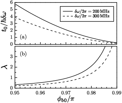
The hopping integral $t_{0}$ can be adjusted in-situ by varying the dc magnetic flux $\phi_{b0}$ between the bottom two junctions. This is illustrated in Fig. 2(a), where the ratio $t_{0}/\hbar\delta\omega$ is shown for $\phi_{b0}/\pi$ between $0.95$ and $0.99$. For the chosen values of $\phi_{b0}/\pi$ we are mainly in the adiabatic regime ($t_{0}>\hbar\delta\omega$), entering the antiadiabatic regime ($t_{0}<\hbar\delta\omega$) for $\phi_{b0}/\pi\approx 0.98$. For the same range of values for $\phi_{b0}$, the effective coupling strength

varies from the weak-coupling to the strong-coupling regime, as can be inferred from Fig. 2(b). For instance, with $\delta\omega/2\pi=200$ MHz and $\phi_{b0}/\pi=0.95$, we have $\lambda=0.34$; for the same value of $\delta\omega$, $\phi_{b0}/2\pi=0.98$ yields $\lambda=2.1$.

Before embarking on a numerical calculation of the ground state of the system, it is worthwhile to analyze the momentum dependence of the vertex function corresponding to the resulting e-ph coupling term:

This vertex function

consists of the $k$- and $q$-dependent SSH part $\gamma_{\mathrm{SSH}}(k,q)=2ig\hbar\delta\omega\>[\sin k-\sin(k+q)]$, and the BM part $\gamma_{\mathrm{BM}}(q)=2ig\hbar\delta\omega\sin q$ that only features $q$ dependence. Since the overall vertex function $\gamma(k,q)$ depends on both $k$ and $q$, it does not belong to the domain of applicability of the Gerlach-Löwen theorem [23], which rules out a nonanalytic behavior of the single-particle quantities. While $k$- and $q$-dependent couplings do not necessarilly lead to nonanalyticities [56], such nonanalyticity indeed occurs in a model with the pure SSH coupling [vertex function $\gamma_{\mathrm{SSH}}(k,q)$] [57]. In the following (see Sec. III.3), we show that the model with combined SSH and BM couplings studied here displays a similar sharp transition between a quasifree excitation and a small polaron.

To determine the ground-state properties of our resulting coupled e-ph model, we employ the conventional Lanczos diagonalization [58] in combination with a controlled truncation of the phonon Hilbert space.

The Hilbert space of the system is spanned by states given as direct products $|n\rangle_{e}\otimes|\mathbf{m}\rangle_{\text{ph}}$. Here, $|n\rangle_{e}=c_{n}^{\dagger}|0\rangle_{e}$ is the state of the excitation localized at the site $n$, $\mathbf{m}=(m_{1},\ldots,m_{N})$ are the phonon occupation numbers, and $|\mathbf{m}\rangle_{\text{ph}}=\prod_{i=1}^{N}(1/\sqrt{m_{i}!})(b_{i}^{\dagger})^{m_{i}}|0\rangle_{\text{ph}}$. Restricting ourselves to a truncated phonon Hilbert space that includes states with at most $M$ phonons (total number on a lattice with $N$ sites), we take into account all $m$-phonon states with $0\leq m_{i}\leq m$, where $m=\sum_{i=1}^{N}m_{i}\leq M$. The dimension of the total Hilbert space is $D=D_{\text{e}}\times D_{\text{ph}}$, where $D_{\text{e}}=N$ and $D_{\text{ph}}=(M+N)!/(M!N!)$.

To further reduce the dimension of the Hamiltonian matrix to be diagonalized, we exploit the discrete translational invariance of our finite system, mathematically expressed as the commutation $[H_{\textrm{eff}},K_{\mathrm{tot}}]=0$ of the Hamiltonian $H_{\textrm{eff}}$ and the total quasimomentum operator $K_{\mathrm{tot}}$. This allows us to perform diagonalization of $H_{\textrm{eff}}$ in sectors corresponding to the eigensubspaces of $K_{\mathrm{tot}}$. For that to accomplish, we make use of the symmetrized basis

where $T_{n}$ denotes (discrete) translation operators. Thus, the dimension of each $K$-sector of the total Hilbert space is $D_{K}=D_{\textrm{ph}}$.

Following an established phonon Hilbert-space truncation procedure [59], the system size ($N$) and the maximum number of phonons retained ($M$) are increased until the convergence for the ground-state energy $E^{(M)}_{\textrm{gs}}$ and the phonon distribution is reached. Our adopted covergence criterion is that the relative error in the ground-state energy and the phonon distribution upon further increase of $N$ and $M$ is not larger than $10^{-4}$. While for the momentum-independent (completely local in real space) Holstein coupling the system size is essentially inconsequential, for nonlocal couplings of the kind studied here this is not the case. In particular, the adopted quantitative convergence criterion is satisfied for the system size $N=10$ (with periodic boundary conditions) and requires the total of $M=8$ phonons.

We now discuss the results obtained by exact diagonalization of our effective model. Unlike more conventional situation, in which the effective coupling strength $\lambda$ [cf. Eq. (21)] is changed by varying the dimensionless coupling constant $g$ (for fixed ratio of the relevant hopping integral and the phonon energy) [8], here we work with a fixed value of $g\delta\omega$ [recall Eq. (20)]. We effectively change $\lambda$ by varying the bare hopping integral $t_{0}$ through the experimentally-tunable parameter $\phi_{b0}$, in accordance with Eq. (12).

Our main finding is that at a critical value of $\phi_{b}$ (i.e., of the effective coupling strength $\lambda$), there is a sharp transition (nonanalyticity) of all relevant quantities [57]. This transition originates from a (real) level crossing and is of first order. It is illustrated in Fig. 3, where the ground-state energy (expressed in units of $\mathcal{E}\equiv\>10^{-3}\>\delta\varphi_{0}^{2}\>E_{J}=2\pi\hbar\times 100$ MHz) is shown as a function of $\phi_{b0}$.

The sharp transition physically corresponds to a change – at a critical value of $\phi_{b0}$ – from a non-degenerate ground state that corresponds to the zero quasimomentum ($K_{\textrm{gs}}=0$), to a twofold-degenerate one corresponding to equal and opposite (nonzero) quasimomenta $K_{\textrm{gs}}$ and $-K_{\textrm{gs}}$. For $\delta\omega/2\pi=200$ MHz this critical value is $(\phi_{b0})_{c}\approx 0.968\>\pi$, while for $\delta\omega/2\pi=300$ MHz we find $(\phi_{b0})_{c}\approx 0.972\>\pi$. The corresponding critical values of the effective coupling strength are $\lambda_{c}\approx 0.83$ and $0.72$, respectively.

Shown in Fig. 4 are two small-polaron Bloch-band dispersions throughout the Brillouin zone (for $\delta\omega/2\pi=200$ MHz and two different values of $\phi_{b0}$), both with band minima (ground states) at nonzero quasimomenta.

For sufficiently strong coupling – e.g., $\phi_{b0}\gtrsim 0.98$ for $\delta\omega/2\pi=200$ MHz – the quasimomentum $K_{\textrm{gs}}$ corresponding to the single-particle ground state saturates at around $\pi/2$ (see the dash-dotted curve in Fig. 4). It should be stressed that – while the ground-state undergoes a sharp transition – the quasimomentum $K_{\textrm{gs}}$ itself varies smoothly between $K_{\textrm{gs}}=0$ and this saturation value as $\phi_{b0}$ is increased beyond its critical value.

Apart from the occurrence of a sharp transition, another interesting aspect of our findings is an effective “compensation” of SSH and BM couplings below the critical value of $\phi_{b0}$. This is indicated in Fig. 3, where the ground-state energy curve essentially follows the bare-dispersion curve $E=-2t_{0}(\phi_{b0})$ all the way up to the critical value of $\phi_{b0}$. This peculiar effect can be ascribed to the character of the resulting momentum dependence of the e-ph vertex function in Eq. (23), being a consequence of the fact that here the SSH and BM coupling strengths are the same [19]. This phenomenon could have profound consequences for transport properties of real electronic systems with competing SSH and BM couplings.

The central quantity for characterizing the small-polaron regime is the quasiparticle residue $Z_{k}\equiv|\langle\Psi_{k}|\psi_{k}\rangle|^{2}$, i.e., the module squared of the overlap between the bare-excitation Bloch state $|\Psi_{k}\rangle\equiv c^{\dagger}_{k}|0\rangle$ and the (dressed) Bloch state $|\psi_{k}\rangle$ of the coupled e-ph system that corresponds to the same quasimomentum ($K=k$). In particular, having determined the ground-state wave function $|{\psi}_{\textrm{gs}}\rangle\equiv|{\psi}_{K=K_{\textrm{gs}}}\rangle$ we can compute $Z_{\textrm{gs}}\equiv Z_{k=K_{\textrm{gs}}}$, a quantity characterizing the ground state of the system. While $Z_{\textrm{gs}}\approx 1$ indicates the weak-coupling regime (quasifree excitation), its reduced values in the strong-coupling regime [see Fig. 5(a)] signify the presence of small polarons, with these two regimes being separated by a nonanalyticity at the critical value of $\phi_{b0}$. It is interesting to note that, unlike for the Holstein model where $Z_{\textrm{gs}}\approx 0$ for strong enough coupling, here $Z_{\textrm{gs}}$ may saturate at a finite value. As can be inferred from Fig. 5(a), for $\delta\omega/2\pi=300$ MHz we find such saturation at $Z_{\textrm{gs}}\approx 0.15$.

Another relevant quantity is the average number of phonons in the ground state

The change of this quantity from values close to zero [see Fig. 5(b)] to a nonzero value $\bar{N}_{\text{ph}}\gtrsim 3$ marks the transition from a quasifree excitation to a small polaron. The aforementioned effective compensation of the SSH and BM couplings below $(\phi_{b0})_{c}$ is reflected in the vanishing phonon-dressing of fermionic excitations, the flat parts of the curves in Fig. 5(b).

The average phonon number $\bar{N}_{\text{ph}}$ is amenable to a direct measurement in our system, through measurements of photon numbers on different resonators (see Sec. IV.2). Likewise, the second moment of the effective phonon distribution can also be extracted by measuring the photon squeezing in the resonators [60, 10]. More generally, the complex multiphononic nature of small-polaron excitations can be fully captured by computing the entire phonon distribution, which is depicted in Fig. 6 for both values of the effective phonon frequency $\delta\omega$ used above. While for $\delta\omega/2\pi=200$ MHz the distribution has a broad maximum at $N_{\textrm{ph}}\approx 4$, the one for $\delta\omega/2\pi=300$ MHz – corresponding to a smaller effective coupling strength $\lambda$ [cf. Eqs. (20) and (21)] – has a weakly-pronounced maximum at around $N_{\textrm{ph}}\approx 1$. By contrast, the dotted curve in Fig. 6, representing a typical phonon distribution for couplings below the critical one, is very strongly peaked at $N_{\textrm{ph}}=0$.

While phonon distributions peaked at zero phonons are characteristic of all small-polaron models in the weak-coupling regime (e.g., below the onset of the polaron crossover in the Holstein model), the peculiarity of our findings is that here such distribution persists all the way up to the critical coupling strength. Although the sharp transitions of the type found here do not result from any kind of cooperative behavior (as is typical for quantum phase transitions in many-particle systems), the observed peculiar behavior allows us to treat $\bar{N}_{\text{ph}}$ as an effective “order parameter” for the predicted sharp transition. Given that $\bar{N}_{\text{ph}}$ is a directly measurable quantity in our system, this fact will facilitate experimental verification of the existence of this transition.

The feasibility of our simulation scheme is contingent upon the ability to prepare the desired small-polaron Bloch states. For this purpose, we make use of the state-preparation protocol proposed in our previous work (Ref. 10), which is only briefly explained in the following.

We assume that the initial state of the system is the vacuum state $|G_{0}\rangle\equiv|0\rangle_{\textrm{e}}\otimes|0\rangle_{\textrm{ph}}$. This state, with no excitations (i.e., with all qubits in their spin-down states) and all resonators in their respective vacuum states, can be prepared via thermalization in a low-temperature environment. Our target state is the dressed-excitation (in the special case, small polaron) Bloch state $\left|\psi_{K}\right\rangle$, corresponding to the eigenvalue $K$ of the total quasimomentum operator $K_{\mathrm{tot}}$.

The microwave driving required for preparing this state is envisioned to be of the form

where $\beta(t)$ describes its time dependence, and the phase factors $e^{\pm iqn}$ indicate that spin-flip operations are applied to different qubits with a $q$-dependent phase difference. It is easy to show that the transition matrix element of the operator $\Omega_{q}(t)$ between the states $\left|G_{0}\right\rangle$ and $\left|\psi_{K}\right\rangle$ is given by [10]

Assuming that $\beta(t)=2\beta_{p}\cos(\omega_{K}t)$, where $\hbar\omega_{K}$ is the energy difference between the states $\left|G_{0}\right\rangle$ and $\left|\psi_{K}\right\rangle$, in the RWA the two states are Rabi-coupled with the effective Rabi frequency $\beta_{p}\sqrt{Z_{K}}$. Thus, starting from the vacuum state $\left|G_{0}\right\rangle$, the state $\left|\psi_{K}\right\rangle$ will be prepared within a time interval of duration [10]

The form of the last expression is consistent with the expectation that the more strongly-dressed states (smaller $Z_{K}$) require longer preparation times. For the small-polaron ground states with $K=\pm K_{\textrm{gs}}$ these preparation times are much shorter than the decoherence time $T_{2}$. For instance, assuming that the pumping amplitude is $\beta_{p}/(2\pi\hbar)=40$ MHz and taking the values for $Z_{\textrm{gs}}$ at the onset of the small-polaron regime [see Fig. 5(a)], we respectively find that $\tau_{\textrm{prep}}\approx 24$ ns for $\delta\omega/2\pi=200$ MHz, and $\tau_{\textrm{prep}}\approx 17$ ns for $\delta\omega/2\pi=300$ MHz. The obtained state-preparation times are three orders of magnitude shorter than currently achievable decoherence times $T_{2}\sim 20-100\>\mu$s of transmon qubits [33, 34], this being a strong indication of the feasibility of our proposed protocol.

The above Rabi-coupling state-preparation protocol, which ensures energy and momentum conservation [10], can in principle be adapted to other systems by taking into account their underlying symmetries. Importantly, the ultimate sucess of this scheme in different systems will depend on the character of their underlying absorption spectra, as described by the corresponding spectral functions (see Sec. V.3). As far as our system is concerned, it should be stressed that the absorption spectra of electronic systems coupled with optical phonons (i.e., phonon modes with a gap in their spectrum) are characterized by generic spectral functions in which the “coherent” part (with a finite spectral weight) is energetically well separated from the incoherent background [61, 12]. This form of absorption spectra should here allow one to avoid inadvertent population of other (excited) states while preparing a desired small-polaron ground state of the system.

Here we discuss the method for measuring the average phonon number $\bar{N}_{\textrm{ph}}$ [cf. Eq. (25)], a quantity which can be thought of as an order parameter for the sharp small-polaron transition (cf. Sec. III.3). As already stressed above, in our implementation $\bar{N}_{\textrm{ph}}$ corresponds to the average total photon number on the resonators. Owing to the discrete translational symmetry of the system, the measurement of $\bar{N}_{\textrm{ph}}$ can be reduced to the measurement of the mean photon number of one of the resonators. This can be accomplished by adding an ancilla qubit which couples to this particular resonator [10], but only during the measurement; this qubit is assumed to be far-detuned from the resonator modes. By measuring the qubit state, the mean photon number on this resonator can be extracted, which multiplied with the total system size $N$ yields the result for $\bar{N}_{\textrm{ph}}$.

As in every other quantum-computation device, decoherence effects should also be present in our simulator. Possible excitations in this system correspond either to flipping of the qubit states or to displacement of the resonator modes, which are subject to the decoherence of the qubits and resonators. In addition to very long dephasing times ($T_{2}\sim 20-100\>\mu$s) of transmon qubits achieved in recent years, for coplanar waveguide resonators the damping time of the microwave photons can reach the same order of magnitude as $T_{2}$, with a quality factor larger than $10^{6}$. The relevant energy scales in our simulator (effective phonon frequency, e-ph coupling strength, and hopping energy) are all of the order of $100$ MHz, far exceeding the decoherence rates. Besides, as shown in Sec. IV.1, even for very strongly-dressed polaron states the typical duration of the state-preparation protocol is three orders of magnitude smaller than the decoherence times. Finally, in the low-temperature environment of our system thermal excitations – which here have energies of a few GHz – can be safely neglected.

The pump pulses of the kind described in Sec. IV.1 may, in principle, induce unwanted transitions (leakage) to higher energy levels in a transmon qubit [62]. Namely, in all qubits based on weakly-anharmonic oscillators leakage from the two-dimensional qubit Hilbert space (computational states) is the leading source of errors at short pulse times [63]. This is especially pronounced if the pulse bandwidth is comparable to the anharmonicity. However, in a typical transmon with $E_{J1}/E_{C1}\sim 50-100$ and a negative anharmonicity of $\sim 3-5\>\%$, even pulses with durations of only a few ns are sufficiently frequency selective that the unwanted transitions can be neglected [28]. In our system, there is an off resonance of around $500$ MHz for such transitions. For a typical driving amplitude $\beta_{p}/2\pi\approx 40$ MHz, the probability of leakage is below one percent, which is a reasonable error rate for the simulator.

Fabrication-related variations in the parameters of Josephson junctions, which are $1-2\>\%$ at best and typically up to $5\>\%$, are unavoidable even in modern-day SC circuits. This is, however, not expected to jeoperdize the observation of the predicted nonanalytic behavior in our system. Namely, as is known from general polaron theory (e.g., the Gerlach-Löwen theorem) the presence of such nonanalyticities (or, more often, the absence thereof) in a particular coupled e-ph model is intimately related to the type of the momentum dependence of the resulting coupling. This momentum dependence, in its own right, depends on the character of the particular coupling mechanisms involved (recall discussions in the introduction and Sec. III.1), rather than on quantitative details such as the magnitude of the bare hopping integral (which in our case is determined by $E_{J}$). Thus the occurrence of the real level crossing which gives rise to the sharp feature in the ground-state energy of the system should be quite robust; the small variations in parameters such as $E_{J}$ can only lead to a slight shift of the critical coupling strength at which this crossing takes place. That this shift is expected to be small – for small variations $\Delta E_{J}$ of the Josephson energy ($\Delta E_{J}/E_{J}\lesssim 5\>\%$) – can be inferred from the expression for the effective coupling strength $\lambda$ [cf. Eq. (21)]. Because $\lambda\propto g^{2}/t_{0}$, where both $g$ and $t_{0}$ depend linearly on $E_{J}$, we have that $\Delta\lambda/\lambda=\Delta E_{J}/E_{J}$.

Generally speaking, dynamical response functions – Fourier transforms of retarded two-time Green’s functions – provide a natural framework for characterizing excitations in many-body systems. The relevant single-particle retarded two-time Green’s function in the problem at hand is given by

where $c_{k}^{\dagger}(t)$ is a single-particle operator in the Heisenberg representation and $[\ldots]_{+}$ stands for an anticommutator. More explicitly, $c_{k}(t)=U^{\dagger}_{H}(t)c_{k}U_{H}(t)$, where $U_{H}(t)$ is the time-evolution operator corresponding to the lab-frame counterpart $H=H(t)$ of our effective Hamiltonian $H_{\textrm{eff}}$ in the rotating frame. The explicit forms of $H$ and $U_{H}$ are not relevant for our present purposes. In fact, the only relevant property of the Hamiltonian $H$ is that its symmetries in the spinless-fermion (pseudospin) sector of the problem are the same as those of the Hamiltonian $H_{\textrm{eff}}$, since this part of $H_{\textrm{eff}}$ preserves its form in the interaction picture.

It should be emphasized that, while the natural Green’s functions for spinless fermions are those that involve anticommutators [cf. Eq. (29)], in the single-particle problem at hand the commutator Green’s function

contains the same physical information. Namely, given that $|\textrm{G}_{0}\rangle$ is a vacuum state, we have that $c_{k}^{\dagger}(t)c_{k}|\textrm{G}_{0}\rangle=0$, which implies that in this special case $G_{-}^{\textrm{R}}(k,t)=-G_{+}^{\textrm{R}}(k,t)$.

Anticipating the use of a real-space experimental probe (see Sec. V.2), we further note that the last momentum-space Green’s function can be retrieved from the real-space resolved ones, i.e.,

where $G_{nn^{\prime}}^{\textrm{R}}(t)\equiv-(i/\hbar)\theta(t)\langle\textrm{G}_{0}|[c_{n}^{\dagger}(t),c_{n^{\prime}}]_{-}|\textrm{G}_{0}\rangle$. By switching to the pseudospin-$1/2$ operators and taking into account that the Jordan-Wigner string operators act trivially on the ground state $|\textrm{G}_{0}\rangle$, these real-space commutator Green’s function can be rewritten as

They can further be transformed to the form

where

and, for simplicity, we suppressed the time argument and the superscript $R$ in the notation for these Green’s functions.

The Ramsey-interference protocol is in principle applicable in any system where single-site addressability is available and yields naturally the real-space and time-resolved commutator Green’s functions of spin operators [64, 65]. In the problem at hand it involves the pseudospin degree of freedom of the transmon qubits.

The general Rabi pulses can be parameterized as

where $\theta=\Omega\tau$, with $\Omega$ being the Rabi frequency and $\tau$ the pulse duration; $\phi$ is the phase of the laser field. The Ramsey protocol makes use of the special case $R_{n}(\phi)\equiv R_{n}(\theta=\pi/2,\phi)$ of such pulses, with $\theta=\pi/2$ and arbitrary $\phi$.

Quite generally, the Ramsey-interference protocol entails the following steps: (1) perform local $\pi/2$-rotation at site $n$ (with $\phi=\phi_{1}$); (2) evolve the system during time $t$; (3) perform local $\pi/2$-rotation at site $n^{\prime}$, or global $\pi/2$-rotation (with $\phi=\phi_{2}$); (4) measure the system in the $\sigma_{z}$ basis at site $n^{\prime}$. In our system, the described protocol leads to the measurement result given by the expectation value

The procedure for extracting relevant Green’s function can be simplified by exploiting the symmetries of our system in the pseudospin sector. Since its Hamiltonian involves a sum of an $XY$-coupling term and $\sigma_{n}^{z}$ terms [recall Eq. (13)], our system has a $U(1)$ symmetry under $z$-axis pseudospin rotations, implying that $\mathcal{G}^{xx}_{nn^{\prime}}=\mathcal{G}^{yy}_{nn^{\prime}}$ and $\mathcal{G}^{xy}_{nn^{\prime}}+\mathcal{G}^{yx}_{nn^{\prime}}=0$. Another symmetry of our system is that under reflections with respect to the $z$ axis ($\sigma_{n}^{x}\rightarrow-\sigma_{n}^{x}$, $\sigma_{n}^{y}\rightarrow-\sigma_{n}^{y}$, $\sigma_{n}^{z}\rightarrow\sigma_{n}^{z}$), which implies that any expectation value involving an odd (total) number of $\sigma_{n}^{x}$ and $\sigma_{n}^{y}$ operators is equal to zero. For a system with these two symmetries, the Ramsey protocol measures [65]

Thus the combinations $\mathcal{G}^{xx}_{nn^{\prime}}+\mathcal{G}^{yy}_{nn^{\prime}}$ and $\mathcal{G}^{xy}_{nn^{\prime}}-\mathcal{G}^{yx}_{nn^{\prime}}$ needed to recover $G_{nn^{\prime}}^{\textrm{R}}(t)$ [recall Eq. (33)] can be obtained by choosing the angles $\phi_{1},\phi_{2}$ such that $\phi_{1}-\phi_{2}=\pm\pi/2$ and $\phi_{1}=\phi_{2}$, respectively.

In the realm of SC qubits, the Ramsey-interference protocol is conventionally used to determine the decoherence time $T_{2}$ of a single qubit, a procedure known as the Ramsey-fringe experiment [34]. The use of this protocol is also envisioned for other types of manipulation, such as interaction-free measurements [66]. In the present work, we propose its use on pairs of qubits in a multi-qubit system, for the purpose of extracting the desired two-time correlation- and Green’s functions.

Provided that the single-particle retarded two-time Green’s function [cf. Eq. (29)] is extracted as explained in Secs. V.1 and V.2, we can also obtain the information about the spectral properties of the system. Namely, by Fourier-transforming this Green’s function to momentum-frequency space, the spectral function is obtained as $A(k,\omega)=-(1/\pi)\textrm{Im}\>G_{+}^{\textrm{R}}(k,\omega)$. The spectral function can quite generally be represented in the form

where $|\psi^{(j)}_{k}\rangle$ is a complete set of total-quasimomentum $k$ eigenstates of the total Hamiltonian of the coupled e-ph system (in our case $H_{\textrm{eff}}$), and $E_{k}^{(j)}$ the corresponding eigenvalues. In the simplest case, the above sum over $j$ includes the polaron-ground state $|\psi^{(j=0)}_{k}\rangle$ at quasimomentum $k$ and its attendant continuum of states that correspond to the polaron with quasimomentum $k-q$ and an unbound phonon with quasimomentum $q$. More generally, with increasing coupling strength there will be multiple coherent polaron bands below the one-phonon continuum (threshold for inelastic scattering) which sets in at energy $E_{gs}+\hbar\omega_{0}$ [61], where $\omega_{0}$ is the relevant phonon frequency (in our case $\delta\omega$). All these coherent (split-off from the one-phonon continuum) polaron states contribute to the above sum along with their respective continua.

The spectral function is intimately related to the dynamics of polaron formation. Let us assume that at $t=0$ a bare-excitation Bloch state with quasimomentum $k$ is prepared and e-ph coupling is turned on (e-ph interaction quench). Then $|\psi(0)\rangle=c^{\dagger}_{k}|0\rangle$ is the state of the system at $t=0$, while at a later time $t$ its state is given by $|\psi(t)\rangle=\sum_{j}e^{-\frac{i}{\hbar}E_{k}^{(j)}t}|\psi_{k}^{(j)}\rangle\langle\psi_{k}^{(j)}|c^{\dagger}_{k}|0\rangle$. It is straightforward to verify that by Fourier-transforming the spectral function to the time domain we obtain the amplitude $\langle\psi(t)|c^{\dagger}_{k}|0\rangle$ to remain in the initial (bare-excitation) state of the system at time $t$ [47]. The corresponding probability $|\langle\psi(t)|c^{\dagger}_{k}|0\rangle|^{2}$ yields the quasiparticle residue at time $t$, thus describing the dynamics of polaron formation.

In our system, the last procedure can be implemented by making use of the state-preparation protocol described in Sec. IV.1 to prepare a bare-excitation Bloch state with quasimomentum $k$ and switching on the qubit-resonator coupling at $t=0$. As a matter of fact, given the character of the polaron formation in our system – where at the critical coupling strength there is an abrupt change from an almost undressed (bare) excitation to a heavilly dressed small polaron – a variation of the tunable parameter $\phi_{b0}$ from slightly below the critical value $(\phi_{b0})_{c}$ to slightly above this value is essentially equivalent to an e-ph interaction quench. This should be the most straightforward way to implement a quench in our system.

Polaron formation is admittedly a very complex dynamical process even in the case of the momentum-independent e-ph coupling [46, 47]. Even the very fundamental question related to the time it takes to form a polaron, as well as a more detailed understanding of how phonon excitations evolve into the correlated phonon cloud of the polaron quasiparticle, are not fully answered to date. In the presence of strongly-momentum dependent e-ph interactions, which even allow for the occurrence of sharp transitions, it should be even more difficult to arrive at a full understanding of this process. Our system, with its unique set of experimental tools, should be very useful in this regard. While the time it takes to form a polaron (after an e-ph interaction quench) should be possible to extract already from measurements of the average phonon number (by measuring the photon number on different resonators), additional characteristics of the polaron-formation dynamics can be unravelled by extracting the spectral function via a Ramsey-interference protocol.

References

- [1] R. P. Feynman, Int. J. Theor. Phys. 21, 467 (1982).
- [2] S. Lloyd, Science , 1073 (1996).
- [3] J. I. Cirac and P. Zoller, Nature Phys. , 264 (2012).
- [4] For a recent review, see I. M. Georgescu, S. Ashhab, and F. Nori, Rev. Mod. Phys. , 153 (2014).
- [5] V. M. Stojanović, T. Shi, C. Bruder, and J. I. Cirac, Phys. Rev. Lett. 109, 250501 (2012a).
- [6] A. Mezzacapo, J. Casanova, L. Lamata, and E. Solano, Phys. Rev. Lett. , 200501 (2012).
- [7] F. Herrera and R. V. Krems, Phys. Rev. A 84, 051401 (2011).
- [8] F. Herrera, K. W. Madison, R. V. Krems, and M. Berciu, Phys. Rev. Lett. 110, 223002 (2013).
- [9] J. P. Hague and C. MacCormick, New J. Phys. , 033019 (); Phys. Rev. Lett. , 223001 (2012).
- [10] F. Mei, V. M. Stojanović, I. Siddiqi, and L. Tian, Phys. Rev. B 88, 224502 (2013).
- [11] L. D. Landau, Z. Phys. , (); S. I. Pekar, Zh. Eksp. Teor. Fiz. , ().
- [12] A. S. Alexandrov and J. T. Devreese, Advances in Polaron Physics (Springer-Verlag, Berlin, 2010).
- [13] S. A. Baily and D. Emin, Phys. Rev. B 73, 165211 (2006).
- [14] K. Agarwal, I. Martin, M. D. Lukin, and E. Demler, Phys. Rev. B 87, 144201 (2013).
- [15] C. P. Adams, J. W. Lynn, Y. M. Mukovskii, A. A. Arsenov, and D. A. Shulyatev, Phys. Rev. Lett. 85, 3954 (2000).
- [16] O. Rösch, O. Gunnarsson, X. J. Zhou, T. Yoshida, T. Sasagawa, A. Fujimori, Z. Hussain, Z.-X. Shen, and S. Uchida, Phys. Rev. Lett. 95, 227002 (2005).
- [17] See, e.g., L. Mathey, D.-W. Wang, W. Hofstetter, M. D. Lukin, and E. Demler, Phys. Rev. Lett. , 120404 (2004); I. E. Mazets, G. Kurizki, N. Katz, and N. Davidson, ibid. , (); F. M. Cucchietti and E. Timmermans, ibid. , (); A. A. Blinova, M. G. Boshier, and E. Timmermans, Phys. Rev. A , 053610 (2013).
- [18] T. Holstein, Ann. Phys. (N.Y.) 8, 343 (1959).
- [19] V. M. Stojanović, P. A. Bobbert, and M. A. J. Michels, Phys. Rev. B 69, 144302 (2004).
- [20] S. Ciuchi and S. Fratini, Phys. Rev. Lett. , 166403 (2011); N. Vukmirović, C. Bruder, and V. M. Stojanović, ibid. , 126407 (2012).
- [21] L. M. Woods and G. D. Mahan, Phys. Rev. B , (2000).
- [22] N. Vukmirović, V. M. Stojanović, and M. Vanević, Phys. Rev. B , 041408(R) (2010); V. M. Stojanović, N. Vukmirović, and C. Bruder, ibid. , 165410 (2010).
- [23] B. Gerlach and H. Löwen, Phys. Rev. B , (); , ().
- [24] C. Slezak, A. Macridin, G. A. Sawatzky, M. Jarrell, and T. A. Maier, Phys. Rev. B , ().
- [25] M. H. Devoret and R. J. Schoelkopf, Science 339, 1169 (2013); J. Q. You and F. Nori, Nature (London) 474, 589 (2011); J. Clarke and F. K. Wilhelm, Nature (London) 453, 1031 (2008).
- [26] A. Wallraff et al., Nature (London) 431, 162 (2004).
- [27] A. Blais, R.-S. Huang, A. Wallraff, S. M. Girvin, and R. J. Schoelkopf, Phys. Rev. A 69, 062320 (2004).
- [28] For an introduction, see S. M. Girvin, in Lecture Notes on Strong Light-Matter Coupling: from Atoms to Solid-State Systems (World Scientific, Singapore, 2013).
- [29] L. DiCarlo et al., Nature (London) , 240 (2009).
- [30] V. M. Stojanović, A. Fedorov, A. Wallraff, and C. Bruder, Phys. Rev. B 85, 054504 (2012b).
- [31] For an overview, see A. A. Houck, H. E. Türeci, and J. Koch, Nature Phys. , 292 (2012).
- [32] S. Schmidt and J. Koch, Ann. Phys. 525, 395 (2013).
- [33] H. Paik et al., Phys. Rev. Lett. 107, 240501 (2011).
- [34] C. Rigetti et al., Phys. Rev. B 86, 100506(R) (2012).
- [35] M. Hohenadler, M. Aichhorn, L. Pollet, and S. Schmidt, Phys. Rev. A 85, 013810 (2012).
- [36] A. A. Gangat, I. P. McCulloch, and G. J. Milburn, Phys. Rev. X 3, 031009 (2013).
- [37] B. Villalonga Correa, A. Kurcz, and J. J. Garcia-Ripoll, J. Phys. B: At. Mol. Opt. Phys. 46, 224024 (2013).
- [38] L. Tian, Phys. Rev. Lett. 105, 167001 (2010).
- [39] Y. Zhang, L. Yu, J.-Q. Liang, G. Chen, S. Jia, and F. Nori, Nature Sci. Rep. , 4083 (2014).
- [40] U. Las Heras, A. Mezzacapo, L. Lamata, S. Filipp, A. Wallraff, and E. Solano, arXiv:1311.7626.
- [41] D. J. Egger and F. K. Wilhelm, Phys. Rev. Lett. 111, 163601 (2013).
- [42] A. Kurcz, A. Bermudez, and J. J. Garcia-Ripoll, arXiv:1310.8173.
- [43] T. L. Schmidt, A. Nunnenkamp, and C. Bruder, New J. Phys. 15, 025043 (2013).
- [44] E. Kapit, Phys. Rev. A 87, 062336 (2013).
- [45] J. Koch et al., Phys. Rev. A , 042319 (2007).
- [46] D. Emin and M. A. Kriman, Phys. Rev. B 34, 7278 (1986).
- [47] L.-C. Ku and S. A. Trugman, Phys. Rev. B 75, 014307 (2007).
- [48] G. Li, B. Movaghar, and M. A. Ratner, Phys. Rev. B 87, 094302 (2013).
- [49] Z. Feng, V. Timoshevskii, A. Mauger, C. M. Julien, K. H. Bevan, and K. Zaghib, Phys. Rev. B 88, 184302 (2013).
- [50] M. H. Devoret, in Quantum Fluctuations, S. Reynaud, E. Giacobino, J. Zinn-Justin, Eds. (Elsevier, Amsterdam, 1997).
- [51] T. P. Orlando and K. A. Delin, Introduction to Applied Superconductivity (Addison-Wesley, Reading, 1991).
- [52] See, e.g., Y. Makhlin, G. Schön, and A. Shnirman, Rev. Mod. Phys. , 357 (2001).
- [53] S. Johnston, F. Vernay, B. Moritz, Z.-X. Shen, N. Nagaosa, J. Zaanen, and T. P. Devereaux, Phys. Rev. B 82, 064513 (2010).
- [54] Z. Radović, N. Božović, and I. Božović, Phys. Rev. B 77, 092508 (2008).
- [55] V. Y. Butko, G. Logvenov, N. Božović, Z. Radović, and I. Božović, Adv. Mat. , 3644 (2009).
- [56] A. Alvermann, D. M. Edwards, and H. Fehske, Phys. Rev. Lett. 98, 056602 (2007).
- [57] V. M. Stojanović and M. Vanević, Phys. Rev. B , 214301 (2008); see also D. J. J. Marchand et al., Phys. Rev. Lett. , 266605 (2010).
- [58] J. K. Cullum and R. A. Willoughby, Lanczos Algorithms for Large Symmetric Eigenvalue Computations (Birkhäuser, Boston, 1985).
- [59] G. Wellein and H. Fehske, Phys. Rev. B 56, 4513 (1997).
- [60] M. Marthaler, G. Schön, and A. Shnirman, Phys. Rev. Lett. 101, 147001 (2008).
- [61] S. Engelsberg and J. R. Schrieffer, Phys. Rev. 131, 993 (1963).
- [62] J. M. Gambetta, F. Motzoi, S. T. Merkel, and F. K. Wilhelm, Phys. Rev. A 83, 012308 (2011).
- [63] See, e.g., R. Fazio, G. M. Palma, and J. Siewert, Phys. Rev. Lett. 83, 5385 (1999).
- [64] G. De Chiara, T. Calarco, S. Fishman, and G. Morigi, Phys. Rev. A 78, 043414 (2008).
- [65] M. Knap, A. Kantian, T. Giamarchi, I. Bloch, M. D. Lukin, and E. Demler, Phys. Rev. Lett. 111, 147205 (2013).
- [66] G. S. Paraoanu, Phys. Rev. Lett. 97, 180406 (2006).
- [67] G. B. Arfken and H. J. Weber, Mathematical Methods for Physicists (Academic Press, San Diego, 2001), 5th ed.