Valid inference from non-ignorable network sampling mechanisms

Let $W$ denote the full data, with distribution $p(W\mid\tau)$, and let $I$ denote a sampling mechanism, i.e., the dynamic process of data collection. We adopt the convention (proposed by (Rubin, 1987)) of using the letter $I$ to also represent the indicator for the data included in the sample. Let $W_{\text{INC}}$ denote the observed data i.e., the elements of $W$ for which $I=1$. The joint distribution of $(W,I)$ is often written as

where $\eta$ represents the tuning parameters of the sampling mechanism. A sampling mechanism $I$ is called ignorable (Rubin (1987)) if

and the parameters for the sampling mechanism ($\eta$) and the full data ($\tau$) are distinct. If a sample mechanism $I$ does not fulfil these conditions, it is called non-ignorable. The condition stated in Equation 2 is called missing at random. If a sampling mechanism is ignorable, then the term corresponding to the distribution of $I$ can be omitted from the likelihood. By this it is meant that the likelihood for $\tau$ is obtained by integrating out the missing data from $p(W\mid\tau)$. In contrast, when the sampling mechanism is non-ignorable, the likelihood for $\tau$ is obtained by integrating out the missing data from $p(W\mid\tau)p(I\mid W,\eta)$.

For the purpose of this paper, it is reasonable to set $W=(Y,\mathcal{G})$, where $\mathcal{G}=(\mathcal{V},\mathcal{E})$ is the graph or social network, with vertex set $\mathcal{V}$ and edge set $\mathcal{E}$, and $Y$ is the vector of univariate responses associated to each node of $\mathcal{G}$. This means that a sampling mechanism $I$ is non-ignorable if its distribution is not constant with respect to unobserved entries of $Y$ or to features of the unobserved portion of the network. Although we are merging $Y$ and $\mathcal{G}$ into $W$, note that conceptually they are quite different entities: $Y$ is the variable of interest for the investigator, while $\mathcal{G}$ provides information regarding the connections among individuals, which can be used to weight the $Y$’s or to suggest a dependence structure i.e., the observed part of $\mathcal{G}$ works as a set of post-sampling covariates. We denote by $\mathcal{G}_{\text{INC}}$ and $\mathcal{G}_{\text{EXC}}$, respectively, the observed and unobserved parts of the network. $Y_{\text{INC}}$ denotes the responses of the individuals that were included in the sample, $Y_{\text{EXC}}$ denotes the responses of the individuals that were not included in the sample.

The notion of amenability discussed in (Handcock and Gile, 2011) is a particular case of the definition of ignorability proposed in (Rubin, 1987). Such notion is useful when the object of the inference is the parameter vector that serves to specify the distribution of $\mathcal{G}$. In this paper, we will adopt Rubin’s definition of ignorability, since it is general enough to encompass the cases where the object of the inference is either:

1. 1.

   A quantity of the form $Q=Q(\tau)$, where $\tau$ serves to specify the distribution of the random graph and the joint distribution of the responses.

2. 2.

   A quantity of the form $Q=Q(\mathcal{G},Y)$, e.g. an average of the response vector weighted by the node degrees.

An estimand of the form $Q=Q(\tau)$ will be used to pose inferential questions at a super-population level (these will be statements in terms of parameters). To pose inferential questions at a population level, we will use an estimand of the form $Q=Q(\mathcal{G},Y)$ (these will be statements about the missing data distribution). Both estimands will be discussed in detail in Section 3.2.

Respondent-Driven Sampling (RDS) is a sampling procedure that takes advantage of the social network structure. It was proposed by Heckathorn (1997). RDS consists of choosing $s$ starting points (individuals identified as nodes of the network) according to a pre-specified mechanism that can be either deterministic or random, and then propagating the sample by following a set of policies defined in terms of the social network. Let $N$ denote $|\mathcal{V}|$, the number nodes for $\mathcal{G}$, $n$ denote the sample size, and $m$ represent the maximum number of referrals per node. Let $D$ denote the vector that has as $i-$th component the degree of the $i-$th vertex, and let $D_{\text{INC}}$ denote the vector of observed degrees. We describe the RDS algorithm in terms of the construction of $(\mathcal{G}_{\text{INC}},Y_{\text{INC}},D_{\text{INC}})$:

1. 1.

   Sample $s$ nodes uniformly from $\mathcal{V}$. This is known as the $0$-th wave. The selected nodes constitute $\mathcal{G}_{\text{INC}[0]}$.

2. 2.

   For each node $i$ in Step (a), record the response $Y(i)$ in $Y_{\text{INC}[0]}$ and the corresponding degree $D(i)$ in $D_{\text{INC}[0]}$.

3. 3.

   For each node in the $(k-1)$-th wave, sample uniformly $m$ nodes among its neighbours relative to $\mathcal{G}$, such that they have not been included in $\mathcal{G}_{\text{INC}}$ already. This is known as the $k$-th wave.

4. 4.

   For each node $i$ sampled in Step (c), record the response $Y(i)$ in $Y_{\text{INC}[k]}$, the corresponding degree $D(i)$ in $D_{\text{INC}[k]}$, and the edge that connected $i$ to $\mathcal{G}_{\text{INC}[k-1]}$ to construct $\mathcal{G}_{\text{INC}[k]}$.

5. 5.

   Repeat Steps (c) and (d) until the pre-specified sample size $n$ has been attained. Interrupt the current wave if necessary.

Let $\eta$ denote the vector of tuning parameters $(m,s,n)$. We use steps (a)-(e) to describe RDS as an algorithm with inputs $(\mathcal{G},Y,\eta)$ and outputs $(\mathcal{G}_{\text{INC}},Y_{\text{INC}},D_{\text{INC}})$. In our notation, $\mathcal{G}_{\text{INC}}$ denotes not only the observed subgraph, but it also encodes the order in which edges were added to it. Observe that Step (a) was set this way in order to ease the exposition. The distribution of the starting points can be modified (in particular, it can be set as a point mass). The description we provided for step (c) is useful when implementing a simulation, however, in practice, it is the individual recruited in the study who selects $m$ out of his/her contacts; neither the statistician nor the practitioner implementing the sampling know, in advance, the list of contacts of any of the individuals involved in the study. Finally, note that, the notion of wave encodes the discrete time involved in the sampling process.

Remember that, in this paper, we follow the convention established by Rubin (1987) of incorporating the uncertainty of the sampling mechanism via its conditional distribution with respect of the full data (Equation 1). In principle, one should write the distribution of RDS as $p(I\mid\mathcal{G},Y,\eta)$. This intuition seems to be validated by the fact that RDS can be seen as a stochastic algorithm with $(\mathcal{G},Y,\eta)$ as inputs. However, from the policies $(a)-(e)$, it follows that the distribution of RDS is constant with respect to the value of $Y$. Therefore, from now on, the distribution of RDS (and any other link-tracing design) will be written as $p(I\mid\mathcal{G},\eta)$.

Let $I$ denote RDS, which is understood as a probabilistic process for gathering data that propagates through a network $\mathcal{G}$. RDS is fully specified by $\eta=(m,s,n)$. The probability distribution for $I$ given $\mathcal{G}$ ($s$ was set equal to 1, to ease the exposition) can be written as:

Here $\tilde{d}_{(\cdot)}$ stands for the number of neighbours (with respect to $\mathcal{G}$) of a given vertex that have not been sampled before it, we refer to it as the adjusted degree; $w_{(\cdot)}$ denotes the number of recruited individuals during the previous wave by a given vertex (clearly, $w_{(\cdot)}\leq m$); while $k$ denotes the number of waves needed to recruit $n$ individuals (such number is a function of the RDS policies and the restrictions imposed by the graph topology).

We assume a data generative model of the form:

This means that we understand $\mathcal{G}$ as a realization of a random graph (statistical network) model with parameter vector $\alpha$. As explained before, the distribution of $I$ is conditional on a given realization of $\mathcal{G}$, it is not necessary to know how the graph was generated to sample $I$ (an assumption of link-tracing designs). Therefore $\alpha$ does not appear on the conditional for $I$. A key assumption of our approach is that $\mathcal{G}$ induces a dependence structure on $Y$. To fully specify such dependence structure, additional parameters may be needed; those parameters are denoted by $\gamma$, that explains the term $p(Y\mid\mathcal{G},\gamma)$. $p(\alpha)$ and $p(\gamma)$ are the priors for $\alpha$ and $\gamma$, respectively.

To simulate from the generative model proposed in Equation 4, first one needs to generate the pair $(\mathcal{G},\alpha)$, then, a realization of $\gamma$ to be able to sample $Y\mid(\mathcal{G},\gamma)$. Once one has $(\mathcal{G},Y)$, the sample mechanism $I$ is applied. In the case of RDS, this produces $(\mathcal{G}_{\text{INC}},Y_{\text{INC}},D_{\text{INC}})$ as the data one would be able to observe.

Observe that we include the factor $p(I\mid\mathcal{G},\eta)$ to deal with non-ignorability issues. Still, to achieve this, we need to model the missing data, which, in this case is given by the underlying graph: that is the purpose of adding the factor $p(\mathcal{G}\mid\alpha)p(\alpha)$. For this paper, we assume that the responses are binary, more specifically, that each $y(i)$ takes values in $\left\{0,1\right\}$. In addition, the factor $p(Y\mid\mathcal{G},\gamma)$ will always be assumed to represent a Markov Random Field (MRF).

Note that Expression 4 is compatible with the factorisation described in Expression 1. Here $W=(Y,\mathcal{G})$ and $\tau=(\alpha,\gamma)$. For the problems discussed in this paper, the sampling mechanism will be driven by tuning parameters $(\eta)$ that are known to the researcher, and therefore, they are not part of the inference. For the sake of simplicity, we do not include covariates, but there is no impediment for incorporating them if needed.

The quantities to be estimated are: the proportion of positive responses at the population and super-population levels. In the context of this paper, each response corresponds to a measurement performed on one of the $N$ individuals associated to the nodes of a network $\mathcal{G}$. We first present the estimand for the super-population inference:

here, the expectation inside the parenthesis is with respect to $p(Y\mid\mathcal{G},\gamma)$ and the one outside the parenthesis is with respect to $p(\mathcal{G}\mid\alpha)$. The estimand associated to the population-level inference is of the form:

where the expectation inside the parenthesis is with respect to $p(Y_{\text{EXC}}\mid\mathcal{G}_{\text{EXC}},\mathcal{G}_{\text{INC}},Y_{\text{INC}})$, while the expectation outside the parenthesis is with respect to $p(\mathcal{G}_{\text{EXC}}\mid\mathcal{G}_{\text{INC}},Y_{\text{INC}})$.

Because of the MRF assumption, to compute the likelihood of $Y_{\text{INC}}$, it is necessary to augment versions of $(Y_{\text{EXC}},\mathcal{G}_{\text{EXC}})$ to the observed data. Augmenting $\mathcal{G}_{\text{EXC}}$ is also a key step for dealing with the non-ignorability of the sampling mechanism (as explained in Sections 2.2 and 3.1). Since we do not know how many nodes and edges were unobserved due to $I$, the model becomes one of variable dimension. For the sampling mechanisms we considered for this paper, the way $\mathcal{G}_{\text{INC}}$ is augmented will have an impact on the factor of the likelihood that includes $I$, i.e., they are non-ignorable.

To perform inference on the model we just proposed we will pursue a Bayesian model averaging (see (Raftery et al., 1996) and (Robert, 2001), Section 7.4) strategy:

In this setting, the mixing distribution $p(\mathcal{G}_{\text{EXC},w},\alpha_{w}\mid\mathcal{G}_{\text{INC}},D_{\text{INC}})$ provides information about the random graph model and an imputation of the underlying network, the posterior $p(\gamma_{w}\mid Y_{\text{INC}},\mathcal{G}_{\text{INC}},\mathcal{G}_{\text{EXC},w})$ encodes what has been learned about the parameter vector driving the dependence structure of the $Y$’s, and $p_{w}(Q_{\bigstar}\mid\alpha_{w},\gamma_{w})$ produces a Monte Carlo version of $Q_{\bigstar}$ given $(\alpha_{w},\gamma_{w})$ (See Expression 5). Here, $w$ indexes the network data imputations implied by $(\mathcal{G}_{{\text{EXC}},w},\alpha_{w})$, where each imputation fixes the dimension of the problem. Equation 7 provides a reasonable strategy for computing the posterior for $Q_{\bigstar}$ as long as reliable inferences on $(\mathcal{G}_{\text{EXC}},\alpha)$ can be performed without resorting to information contained in $Y_{\text{INC}}$. Here $\Gamma(\cdot,\cdot,\cdot)$ denotes the set of values $\gamma$ that imply a valid probability model for $Y$, given an imputed network.

So far, we have referred to $\mathcal{G}_{\text{EXC}}$ as the ‘unobserved part of the network’, however, to perform the computations implied by Equation 7, more precision is required. Given $\mathcal{G}_{\text{INC}}$ and $N$ (the maximum allowed size for an imputed network), $\mathcal{G}_{\text{EXC}}$ is given by a set of nodes $\left\{n+1,n+2,\dots,N_{*}\right\}$, where $N_{*}\leq N$ and a set of edges for an adjacency matrix with $N_{*}$ nodes, such that: (i) the edges incident to nodes in $\left\{1,2,\dots,n\right\}$ only, are not included in $\mathcal{G}_{\text{INC}}$; (ii) each of the connected components of the network $\mathcal{G}$ obtained by adding the edges of $\mathcal{G}_{\text{INC}}$ to $\mathcal{G}_{\text{EXC}}$ has a non-empty intersection with $\left\{1,2,\dots,n\right\}$.

To sample from $p(\mathcal{G}_{\text{EXC}},\alpha\mid\mathcal{G}_{\text{INC}},D_{\text{INC}})$, we propose constructing a Gibbs sampler based on the full conditionals

The explicit form of such conditionals will be given by the modelling choices for $p(\alpha)p(\mathcal{G}\mid\alpha)$ and the constrains imposed by $p(I\mid\mathcal{G},\eta)$. In an analogous manner, to sample from the posterior for $\gamma$, we impute $Y_{\text{EXC}}$ and construct a Gibbs sampler based on the full conditionals

Because we assume a MRF for $p(Y\mid\mathcal{G},\gamma)$, sampling from the full conditional

usually involves dealing with a distribution with an intractable partition function (See Møller et al. (2006)); this will be discussed with more detail in Section 4.2.

We now present the specific choices we made for these distributions: For $\mathcal{G}$ an Erdös-Rényi model Erdos and Renyi (1960) was assumed, with a single probability of inclusion $\alpha\in(0,1)$. A Beta$(\omega_{1},\omega_{2})$ was used as prior for $\alpha$. Our specification for $p(I\mid\mathcal{G},\eta)$ is an RDS with $\eta=(m,s,n)$ (i.e., RDS is specified with $m$ coupons per wave, $s$ seeds and sample size $n$). For the vector of responses $Y$, we assumed the Markov Random Field (MRF) implied by:

here

where $A_{\mathcal{G}}$ denotes the adjacency matrix for $\mathcal{G}$ and $\gamma=(\gamma_{0},\gamma_{1})$. As suggested in Møller et al. (2006), we assume a uniform prior on $\gamma$ of the form:

We adopt these distributions for the sake of concreteness; they are not essential to our methodology. Any sampling design that propagates through a social network could be used to specify $p(I\mid\mathcal{G},\eta)$. In principle, we could use any random graph model for $p(\mathcal{G}\mid\alpha)$, as long as:

1. 1.

   The density of the random graph model can be computed efficiently.

2. 2.

   It is feasible to marginalise efficiently, this is, to obtain the distribution of $\mathcal{G}_{\text{INC}}$ given any realization of $I$.

For instance, one may also consider the following prior:

which is inspired by the model proposed by Perry and Wolfe (2012).

In Section 3.3, we proposed a general strategy for sampling from the posterior for $Q_{\bigstar}(\alpha,\gamma)$ (or $Q_{\circ}(\mathcal{G}_{\text{INC}},Y_{\text{INC}})$) conditional on $(\mathcal{G}_{\text{INC}},Y_{\text{INC}},D_{\text{INC}})$. Such strategy is based on a Bayesian model averaging (BMA) approach (Equation 7) where samples from the mixing distribution and from the posterior for $\gamma$ given $(\mathcal{G}_{\text{INC}},\mathcal{G}_{\text{EXC}},Y_{\text{INC}})$ are obtained via Gibbs-Sampler schemes. In this section, we discuss how to sample from the full conditionals implied by these schemes for the choices outlined in Section 4.1. Since we will often deal with regimes where $N$ is at least twice bigger than $n$, and therefore, the number of entries of the adjacency matrix that we do not fully observe will be much larger than the number of entries available from $\mathcal{G}_{\text{INC}}$, we opted for proposals such that encourage imputations for $(\mathcal{G}_{\text{EXC}},Y_{\text{EXC}})$ such that they do not differ too much from $(\mathcal{G}_{\text{INC}},Y_{\text{INC}})$ from a qualitative point of view.

We first introduce some notation: Let $\mathcal{V}_{\text{INC}}$ and $\mathcal{V}_{\text{EXC}}$ the set nodes of $\mathcal{G}_{\text{INC}}$ and its complement. Let $\bar{Y}_{\text{INC}}$ denote the sample mean computed from the entries of $Y_{\text{INC}}$. Denote by $A_{\mathcal{H}}$ the submatrix of $A_{\mathcal{G}}$ (the adjacency matrix for $\mathcal{G}$) obtained by taking only the rows associated to elements of $\mathcal{V}_{\text{INC}}$. We denote by $b_{O}$ the number of zeros in submatrix of $A_{\mathcal{G}}$ obtained by taking the rows associated to $\mathcal{V}_{\text{INC}}$ and the columns associated to $\mathcal{V}_{\text{EXC}}$. Denote by $j_{I}$ the number of edges included in $\mathcal{G}_{\text{INC}}$. Let $\alpha_{\text{LOW}}$ and $\alpha_{\text{UP}}$ denote, respectively, the minimum and maximum values for the density of that submatrix, given the constrains imposed by $D_{\text{INC}}$.

To sample from $p(\mathcal{G}_{\text{EXC}}\mid\alpha,\mathcal{G}_{\text{INC}},D_{\text{INC}})$ we implemented a Metropolis step based on a mixture of four kernels. The first kernel corresponds to a proposal where a vertex $v\in\mathcal{V}_{\text{INC}}$ is picked uniformly at random, and all the edges connecting it to elements of $\mathcal{V}_{\text{EXC}}$ are re-wired, so the number of neighbours of $v$ belonging to $\mathcal{V}_{\text{EXC}}$ remains constant. The Metropolis ratio implied by these choices has the form

where $p(I\mid\mathcal{G}_{\text{INC}},\mathcal{G}_{\text{EXC}}^{(\cdot)},\eta)$ is the value of Equation 3 that results from using the imputation of the network implied by $\mathcal{G}_{\text{EXC}}^{(\cdot)}$. Note that, this move keeps the number of edges constant, therefore the terms corresponding to the Erdös-Rényi probability mass function cancel out. Clearly, the move that reverses the proposed one implies picking the same $v\in\mathcal{V}_{\text{INC}}$. By conditioning on this event, the proposal becomes a uniform over the subsets of $\mathcal{V}_{\text{EXC}}$ that have as many elements as v has neighbours in $\mathcal{V}_{\text{EXC}}$. This last statement implies that the terms corresponding to the proposal also cancel out. The second and third kernels should be seen as dual: the second kernel corresponds to the proposal where an edge connecting to vertices $(v,w)\in\mathcal{V}_{\text{INC}}\times\mathcal{V}_{\text{INC}}$ is chosen uniformly at random and then substituted by two edges, each of them connecting a different element of $\left\{v,w\right\}$ with an element of $\mathcal{V}_{\text{EXC}}$ (not necessarily the same one) picked uniformly at random. The third kernel allows for the opposite move: it takes two vertices $(v,w)\in\mathcal{V}_{\text{INC}}\times\mathcal{V}_{\text{INC}}$ such that, each of them has at least one edge connecting it to an element of $\mathcal{V}_{\text{EXC}}$, then, two of such edges are chosen (one incident to $v$ and one incident to $w$) uniformly at random and then replaced by an edge connecting $v$ and $w$. Let $h_{I}^{(\cdot)}$ be the number of edges of the form $(v,w)\in\mathcal{V}_{\text{INC}}\times\mathcal{V}_{\text{INC}}$ that are in the current version of the network due to imputation (i.e., these edges were not observed). The Metropolis ratio corresponding to the second kernel is of the form

while the Metropolis ratio for the third kernel is given by

The fourth kernel corresponds to the proposal where the submatrix of $A_{\mathcal{G}}$ with rows and columns associated to $\mathcal{V}_{\text{EXC}}$ is imputed using independent draws from a Bernoulli with probability of success $\alpha$. This proposal implies the Metropolis ratio

since the terms corresponding to the proposal and those corresponding to the random graph distribution (given $\alpha$) cancel out.

To sample from $p(\alpha\mid\mathcal{G}_{\text{EXC}},\mathcal{G}_{\text{INC}},D_{\text{INC}})$ we implemented a Metropolis step based on a mixture of two kernels. The first kernel corresponds to a Beta$(\kappa_{1},\kappa_{2})$ proposal, where

The intuition behind this proposal is the following: this distribution can be understood as the posterior for $\alpha$ implied by the Jeffreys prior, Beta$(0.5,0.5)$, and the counts for presence and absence of edges in the submatrix of $A_{\mathcal{G}}$ obtained by taking only the rows corresponding to elements of $\mathcal{V}_{\text{INC}}$. By adopting this proposal, the Metropolis ratio required for computing the acceptance probability for a new move $\alpha^{(t)}$ takes the form:

where $h_{\mathcal{G}}$ denotes the number of non-zero entries of the upper-triangular part of $A_{\mathcal{G}}$. The second kernel corresponds to a Beta$(\zeta_{1},\zeta_{2})$ proposal, where $\zeta_{1}$ and $\zeta_{2}$ are such that, the $5$ and $95$% quantiles of this Beta distribution are equal to $\alpha_{\text{LOW}}$ and $\alpha_{\text{UP}}$, respectively. The Metropolis ratio implied by this proposal has the same form as the one shown in Equation 11, one just needs to replace $(\kappa_{1},\kappa_{2})$ by $(\zeta_{1},\zeta_{2})$.

To sample from $p(Y_{\text{EXC}}\mid\gamma,Y_{\text{INC}},\mathcal{G}_{\text{INC}},\mathcal{G}_{{\text{EXC}}})$, we use a Metropolis step with proposal $q(Y_{\text{EXC}})$ given by a multivariate Bernoulli with all marginal probabilities of success equal to $\bar{Y}_{\text{INC}}$ and such that its components are independent. To accept a new proposed value $Y_{\text{EXC}}^{(t)}$, we compute the following Metropolis ratio:

where $V_{0}^{(\cdot)}$ and $V_{0}^{(\cdot)}$ are, respectively, the values of $V_{0}$ and $V_{1}$ implied by $Y_{\text{EXC}}^{(\cdot)}$. Here $c^{(\cdot)}$ denotes the number of non-zero entries of $Y_{\text{EXC}}^{(\cdot)}$.

To sample from $p(\gamma\mid Y_{\text{EXC}},Y_{\text{INC}},\mathcal{G}_{\text{INC}},\mathcal{G}_{{\text{EXC}}})$ using a Metropolis step, we have to deal with the presence of intractable partition functions on a Metropolis ratio. To tackle this task, we follow the approach proposed by Andrieu and Roberts (2009), which is based on using an unbiased estimate of the density function within the Metropolis ratio; more specifically, we implemented the Annealed Importance Sampling (AIS) algorithm (See Neal (2001) and Section 3.2 of Salakhutdinov (2008)) to compute unbiased estimates of the partition function whenever needed. We describe the AIS algorithm briefly in Appendix A. We used a mixture of kernels to update $\gamma$. Each element of the mixture corresponds to a random walk (as described in Section 7.5 of Robert and Casella (2004)) for one of the components of $\gamma$; more specifically, the proposals are based on perturbations of $\gamma_{0}^{(t)}$ (or $\gamma_{1}^{(t)}$) generated from a uniform on $[-\upsilon,\upsilon]$. We consider random walks with reflection on the boundary. These choices imply Metropolis ratios of the form

where $\hat{Z}(\gamma_{0}^{(\cdot)},\gamma_{1})$ denotes the estimate of the partition function computed by AIS and implied by $\gamma_{0}^{(\cdot)}$. Note that we are showing the Metropolis ratio for an update for $\gamma_{0}$, the ratio for performing an update on $\gamma_{1}$ is obtained mutatis mutandis.

We conducted a simulation study to gain better understanding of the performance of our method. First we considered regimes where the random graph model $p(\mathcal{G}\mid\alpha)p(\alpha)$ matches the mechanism that generated the data. To evaluate performance of point estimators, Monte Carlo estimates of the bias and the mean square error (MSE) were computed; to evaluate confidence intervals and credible regions, the frequency of coverage was used. The regimes for the simulation were determined by the following factors:

1. 1.

   The density of the underlying network. We considered the values $0.005$ and $0.01$.

2. 2.

   The size of the underlying network. We considered the values $500$, $1000$ and $2000$.

3. 3.

   The dependence among the entries of the response vector induced by the Markov random field. We considered $\gamma_{1}\in\left\{0.001,0.25\right\}$. The value $\gamma=0.001$ defines regimes with low dependence among the responses; in contrast, $\gamma=0.25$ defines the regimes with high dependence. For each regime, we specify $\gamma_{0}$ by finding the value $\gamma_{0}^{*}$ such that Equation 5 holds, given $(\alpha,\gamma_{1},Q_{\bigstar})$.

The sample size was set as $150$. An Erdös-Rényi model was used to generate the random graph data for all regimes. We set $Q_{\bigstar}=0.2$ for all scenarios. Our method was implemented using the distributions described in Section 4.1. We compared our methodology to the Volz-Heckathorn estimator and the corresponding Bootstrap confidence interval. Results are summarised in Table 1. We observed that, for most regimes, the estimator for $Q_{\bigstar}$ implied by our method had less bias than the VH estimator. In terms of MSE, the VH estimator outperforms the Bayesian estimator when the dependence among the responses is low; in contrast, the estimator implied by our method outperforms the VH estimator when the dependence among the responses is high.

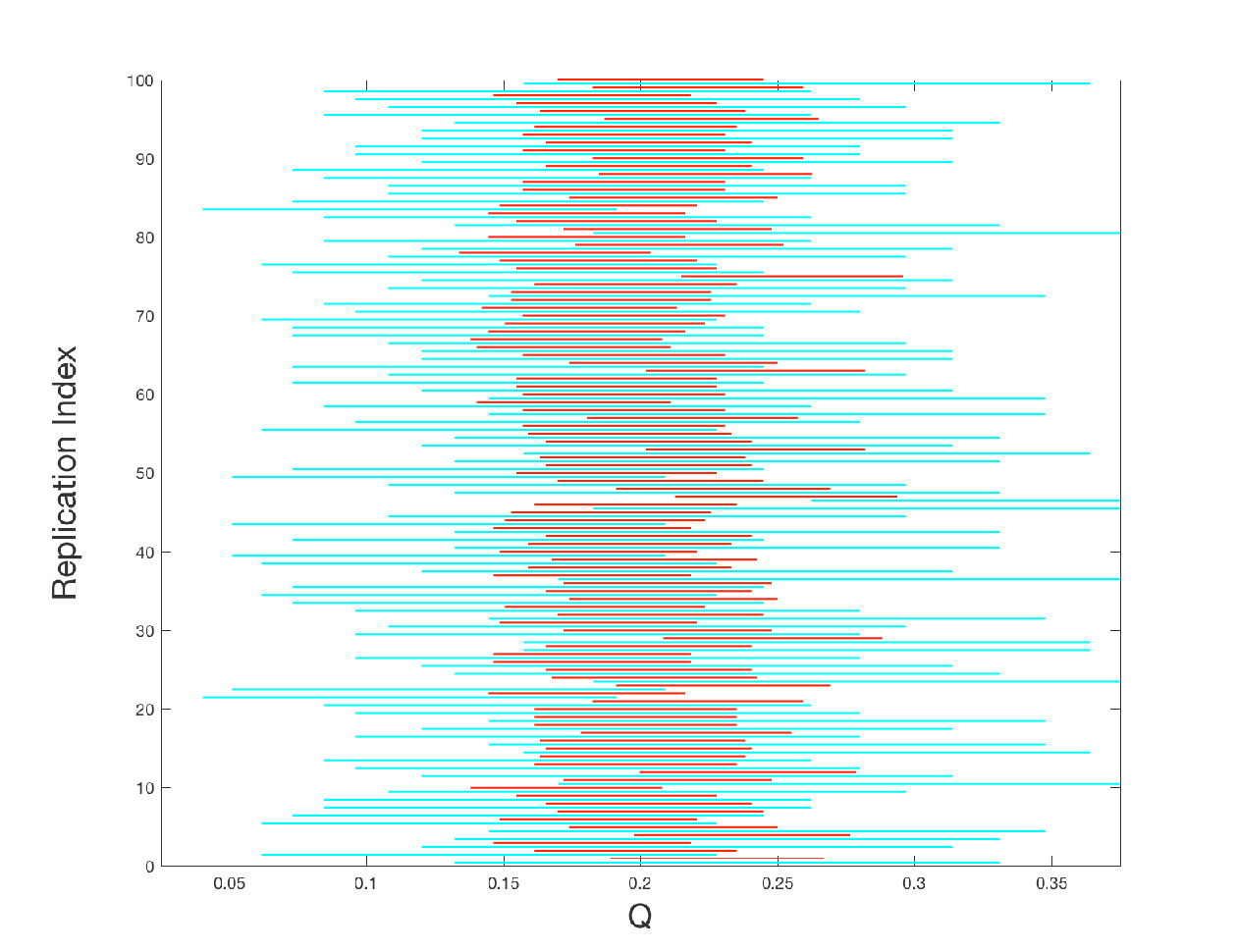
For a given regime (namely, $N=1000$, $\alpha=0.001$, $\gamma=(-0.6927,0.001)$), we plotted the $95$ per cent credible intervals associated to each simulation and the corresponding $95$ per cent confidence intervals implied by bootstrapping Volz-Heckathorn (Figure 2). While both procedures generate estimates with similar bias and coverage, our method produces intervals that are at least half shorter in average. We also plotted the coverage against the average length of the (confidence or credible) interval for each method considering a the same set of regimes used in Tables 1. Results are displayed in Figure 3.

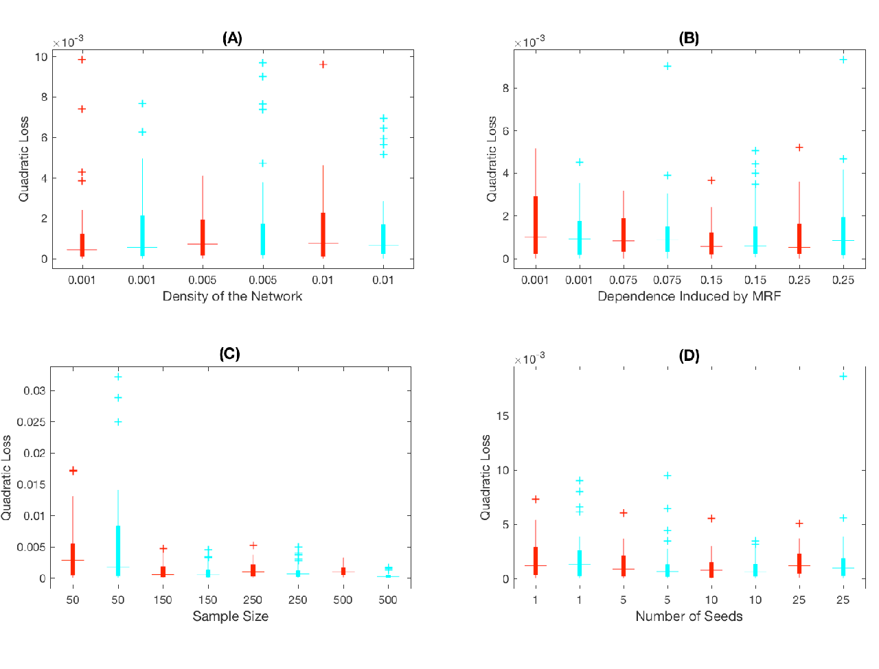
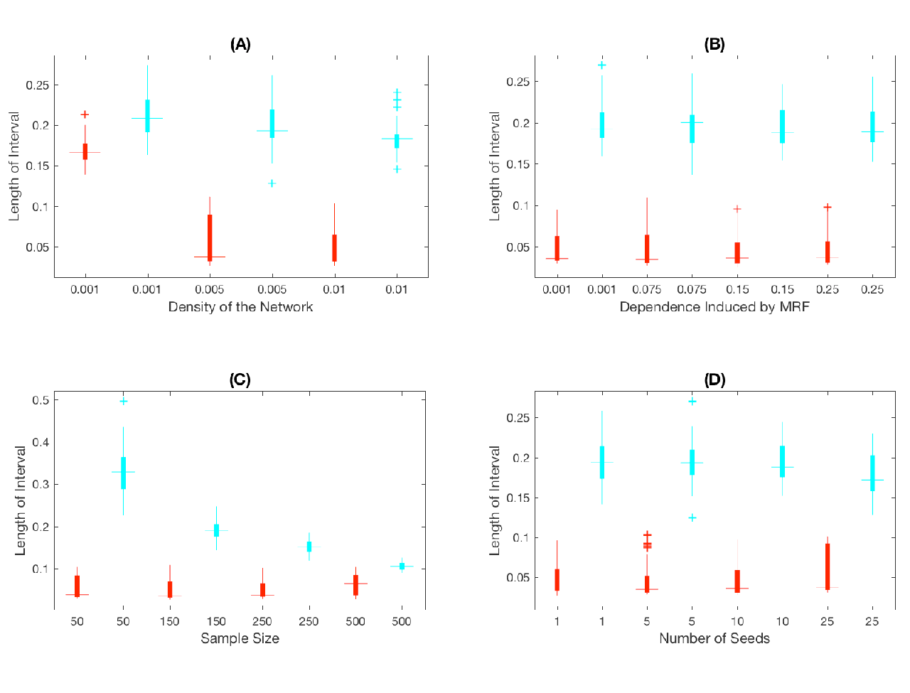
We performed a second set of simulations, again specifying $Q_{\bigstar}=0.2$. We compared our method to the VH estimator in terms of the distribution of quadratic loss $(Q_{\bigstar}-\hat{Q}_{\bigstar})^{2}$ and the distribution of the length of credible/confidence intervals. For this simulation we set $N=1000$ and $m=3$ for all regimes; $\gamma_{1}=0.15$ unless stated otherwise. The regimes we considered for these simulations are defined in terms of density of the underlying network ($\alpha\in\left\{0.001,0.005,0.01\right\}$, panel (A)), dependence among the responses ($\gamma_{1}\in\left\{0.001,0.075,0.15,0.25\right\}$, panel (B)), sample size ($n\in\left\{50,150,250,500\right\}$, panel (C)) and the number of seeds ($s\in\left\{1,5,10,25\right\}$, panel (D)). Results from this simulation are summarised in Figures 4 and 5. As in the previous simulation experiment, we observed that, in terms of quadratic loss, there are no substantial differences between our method and VH. We also observed that, the credible intervals were much shorter than the corresponding confidence intervals, while keeping the coverage close to the nominal value.

We performed one more simulation study where we considered regimes for which the prior $p(\mathcal{G}\mid\alpha)p(\alpha)$ had different functional form from the mechanism that generated the data. We evaluated the procedures using the same criteria as in the experiments described in Section 4.3. The regimes for the simulation are displayed in Table 2; these were determined by the following factors:

1. 1.

   The random graph model used to generate the underlying network was Small World with density $\xi\in\left\{0.005,0.01,0.05\right\}$ and probability of re-wiring $\vartheta\in\left\{0.01,0.25\right\}$.

2. 2.

   The random graph models used to fit the model were Erdös-Rényi.

3. 3.

   The dependence among the responses we determined by $\gamma_{1}\in\left\{0.001,0.25\right\}$.

The values for $\gamma_{0}$ were set up so $Q_{\bigstar}=0.2$ for all regimes. For this simulation, the size of the network was set as $N=1000$, the sample size as $n=150$, the number of referrals as $m=3$ and the number of seeds as $s=1$. Again, our method was implemented using the distributions described in Section 4.1. Results are summarised in Figures 6 and 7. As in the simulations performed in Section 4.3, our method gets similar results to VH in terms of quadratic loss. The regimes that prove harder for both methods, in terms of quadratic loss, are the ones with high dependence and high density of the network (Regimes 4 and 8 in Table 2). We also observed that the credible intervals implied by our method tend to be much shorter than the corresponding Bootstrap confidence intervals, as in the results obtained in Section 4.3. For both methods and all regimes, the coverage of the intervals (credible or frequentist) were close to the nominal value.

To assess the goodness of fit of out model we made use of posterior predictive checks (See (Gelman et al., 1996) and the appendix), i.e., we selected a summary of the observed data and plotted the observed value of this summary against the distribution of replicates of such summary under the posterior predictive distribution. For this case, we used the sample mean of the observed $Y$’s as the summary. Results are displayed in Figure 8. The plot does not show evidence against the goodness of fit of our model.

References

- Andrieu and Roberts (2009) Andrieu, C. and G. O. Roberts (2009). The pseudo-marginal approach for efficient monte carlo computations. The Annals of Statistics 37(2), 697–725.
- Aronow and Crawford (2015) Aronow, P. and F. Crawford (2015). Nonparametric identification for respondent-driven sampling.
- Blitzstein and Nesterko (2012) Blitzstein, J. and S. Nesterko (2012). Bias-variance and breath-depth tradeoffs in respondent-driven sampling.
- de Mello et al. (2008) de Mello, M., A. Pinho, M. Chinaglia, W. Tun, A. Barbosa Junior, and M. Ilario (2008). Assessment of risk factors for hiv infection among men who have sex with men in the metropolitan area of campinas city, brazil, using respondent-driven sampling. Technical report, Washington DC: Population Council.
- Erdos and Renyi (1960) Erdos, P. and A. Renyi (1960). The evolution of random graphs. Magyar Tud. Akad. Mat. Kutato Int. Kolz 5, 17–61.
- Gelman et al. (1996) Gelman, A., X.-L. Meng, and H. Stern (1996). Posterior predictive assessment of model fitness via realized discrepancies. Statistica Sinica 6, 733–807.
- Gile et al. (2015) Gile, K., J. L., and M. Salganik (2015). Diagnostics for respondent-driven sampling. J. R. Statist. Soc. A 178, 241–269.
- Gile (2011) Gile, K. J. (2011). Improved inference for respondent-driven sampling data with application to hiv prevalence estimation. Journal of the American Statistical Association 106, 135–146.
- Handcock and Gile (2011) Handcock, M. S. and K. J. Gile (2011). Modeling social networks from sampled data. The Annals of Applied Statistics 4, 5–25.
- Heckathorn (1997) Heckathorn, D. D. (1997). Respondent-driven sampling: A new approach to the study of hidden populations. Social Problems 44, 174–199.
- Heckathorn (2007) Heckathorn, D. D. (2007). Extensions of respondent-driven sampling: Analyzing continuous variables and controlling for differential degree. Sociological Methodology 37, 151–207.
- Heitjan and Rubin (1991) Heitjan, D. and D. B. Rubin (1991). Ignorability and coarse data. Annals of Statistics 19, 2244–2253.
- Hoff et al. (2002) Hoff, P. D., A. E. Raftery, and M. S. Handcock (2002). Latent space approaches to social network analysis. Journal of the American Statistical Association 97(460), 1090–1098.
- Møller et al. (2006) Møller, J., A. N. Pettitt, R. Reeves, and K. K. Berthelsen (2006). An efficient markov chain monte carlo method for distributions with intractable normalising constants. Biometrika 93(2), 451–458.
- Neal (2001) Neal, R. (2001). Annealed importance sampling. Statistics and Computing 11, 125–139.
- Orbest (2012) Orbest, M. (2012). A question of degree: Sources of uncertainty in respondent driven sampling.
- Perry and Wolfe (2012) Perry, P. and P. Wolfe (2012). Null models for network data.
- Raftery et al. (1996) Raftery, A., D. Madigan, and C. Volinsky (1996). Accounting for model uncertainty in survival analysis improves predictive performance (with discussion). Volume 5 of Bayesian Statistics, pp. 323–349. Oxford University Press.
- Robert (2001) Robert, C. P. (2001). The Bayesian Choice, Second Edition. Springer-Verlag.
- Robert and Casella (2004) Robert, C. P. and G. Casella (2004). Monte Carlo Statistical Methods, Second Edition. Springer-Verlag.
- Rubin (1976) Rubin, D. B. (1976). Inference and missing data. Biometrika 63, 581–592.
- Rubin (1987) Rubin, D. B. (1987). Multiple Imputation for Nonresponse in Surveys. John Wiley and Sons.
- Salakhutdinov (2008) Salakhutdinov, R. (2008). Learning and evaluating boltzmann machines.
- Salganik and Heckathorn (2004) Salganik, M. J. and D. D. Heckathorn (2004). Sampling and estimation in hidden populations using respondent driven sampling. Sociological Methodology 34, 193–239.
- Volz and Heckathorn (2008) Volz, E. and D. D. Heckathorn (2008). Probability based estimation theory for respondent driven sampling. Journal of Official Statistics 24, 79–97.
Appendix A Annealed Importance Sampling
The simple importance sampling algorithm (SIS) is an easy to implement algorithm which provides unbiased estimates for partition functions. However, it suffers from the drawback of potentially producing estimates with infinite variance. It can also perform poorly if the instrumental distribution is very different from the target distribution.
To overcome these difficulties, Neal (2001) proposed the annealed importance sampling (AIS) algorithm. This algorithm requires a finite set of functions that serve as a ‘bridge’ from the instrumental to the target distribution. In this paper, we implemented AIS using the following set of functions
to set a bridge from the instrumental distribution to the target . Here . For this algorithm, it is required that the partition function of the instrumental distribution is easy to compute. To implement AIS, one also requires a set of transition operators such that, each has as its invariant distribution. These operators take a (putative) Monte Carlo sample from as input and produce a sample from a distribution that approximates as output.
We now outline the AIS algorithm:
- 1.
Simulate
- •
from ;
…
from .
- 2.
Compute
for .
- 3.
Use the values from (b) as weights for an importance sampling algorithm to obtain
where is the point estimate for the partition function of the target distribution.
A strong argument for using AIS over SIS, is that, for large values of , the variance of is proportional to .
Appendix B More on Simulations
We fitted an ANCOVA model to assess if the method used to estimate the interval was significant when regarded as a factor. For the case where the model is correctly specified (in terms of random graph model) the other factors to be considered are the size of the network and the density. The response variable is the coverage for the super population parameter . Results are summarized in Table 5.
We also fitted an ANCOVA for the case where the model is unspecified (in terms of random graph model) the other factor to be considered was the density. The response variable is the coverage for the super population parameter . Results are summarized in Table 6.
Factor DF Sum Sq Mean Sq F Value factor(TheMethod) 1 0.0016000 0.00160000 8.7549 0.011946 * TheSize 1 0.0000250 0.00002500 0.1368 0.717934 TheDensity 1 0.0023569 0.00235693 12.8966 0.003705 ** Residuals 12 0.0021931 0.00018276
Factor DF Sum Sq Mean Sq F Value factor(TheMethod) 1 0.0025000 0.0025000 7.1104 0.020542 * factor(TheRG) 1 0.0042250 0.0042250 12.0165 0.004661 ** TheDensity 1 0.0004308 0.0004308 1.2253 0.290018 Residuals 12 0.0042192 0.0003516