When and By How Much Can Helper Node Selection Improve Regenerating Codes?
Abstract
Regenerating codes (RCs) can significantly reduce the repair-bandwidth of distributed storage networks. Initially, the analysis of RCs was based on the assumption that during the repair process, the newcomer does not distinguish (among all surviving nodes) which nodes to access, i.e., the newcomer is oblivious to the set of helpers being used. Such a scheme is termed the blind repair (BR) scheme. Nonetheless, it is intuitive in practice that the newcomer should choose to access only those “good” helpers. In this paper, a new characterization of the effect of choosing the helper nodes in terms of the storage-bandwidth tradeoff is given. Specifically, answers to the following fundamental questions are given: Under what conditions does proactively choosing the helper nodes improve the storage-bandwidth tradeoff? Can this improvement be analytically quantified?
This paper answers the former question by providing a necessary and sufficient condition under which optimally choosing good helpers strictly improves the storage-bandwidth tradeoff. To answer the latter question, a low-complexity helper selection solution, termed the family repair (FR) scheme, is proposed and the corresponding storage/repair-bandwidth curve is characterized. For example, consider a distributed storage network with total number of nodes and the network is resilient against node failures. If the number of helper nodes is , then the FR scheme and its variant demonstrate reduction in the repair-bandwidth when compared to the BR solution. This paper also proves that under some design parameters, the FR scheme is indeed optimal among all helper selection schemes. An explicit construction of an exact-repair code is also proposed that can achieve the minimum-bandwidth-regenerating point of the FR scheme. The new exact-repair code can be viewed as a generalization of the existing fractional repetition code.
Index Terms:
Distributed storage, regenerating codes, family repair schemes, helper nodes, generalized fractional repetition codes, network codingI Introduction
The need for storing very large amounts of data reliably is one of the major reasons that has pushed for distributed storage systems. Examples of distributed storage systems include data centers [6] and peer-to-peer systems [18, 2]. One way to protect against data loss is by replication coding, i.e, if a disk in the network fails, it can be replaced and its data can be recovered from a replica disk. Another way is to use maximum distance separable (MDS) codes. Recently, regenerating codes (RCs) and its variants [4, 24, 15, 19] have been used to further reduce the repair-bandwidth of MDS codes.
One possible mode of operation is to let the newcomer, the node that replaces the failed node, always access/connect to all the remaining nodes. On the other hand, under some practical constraints we may be interested in letting the newcomer communicate with only a subset of the remaining nodes [12], termed the helpers. For example, reducing the number of helpers decreases I/O overhead during repair and thus mitigates one of the performance bottlenecks in cloud storage systems. In the original storage versus repair-bandwidth analysis of RCs [4], it is assumed that the newcomer does not distinguish/choose its helpers. We term such a solution the blind repair (BR) scheme. Nonetheless, it is intuitive that the newcomer should choose to access only those “good” helpers of the remaining nodes. In fact, this idea of selecting good helpers exists even in replication codes, the simplest redundancy technique in the earliest literature of distributed storage systems.
To illustrate this, we consider a storage network with nodes numbered from to . Suppose that we would like to protect against one node failure by replication. To that end, we first divide the file into two fragments, fragments and , and we store fragment in node and fragment in node . Each fragment is replicated once by storing a copy of fragment in node and a copy of fragment in node . If any one of the four nodes fails, then we can retrieve the entire file by accessing the intact fragments and in the remaining three nodes. The repair process of this replication scheme is also straightforward. Say node fails, the newcomer simply accesses node and restores fragment . We observe that the newcomer only accesses the good helper (the one that stores the lost fragment) in this replication scheme. In this scheme, each node stores half of the file, and during the repair process, the newcomer accesses helper node and communicates half of the file. For comparison, if we apply the analysis of [4] (also see our discussion in the next paragraph), we will see that if we use RCs to protect against one node failure, each node has to store the whole file and during the repair process, the newcomer accesses helper and communicates the entire file. The simplest replication code is twice more efficient than RCs in this example.11 1 One may think that this performance improvement over the blind repair (BR) scheme [4] is due to that the parameter values are beyond what is originally considered for the regenerating codes (which requires ). In Appendix A and Section III, we provide other examples with and , respectively, which show that a good helper selection can strictly outperform the BR solution in [4] for as well.
The reason why the replication code is the superior choice in the above example is that it only chooses the good helpers during the repair process, while the analysis in [4] assumes a blind helper selection.22 2 Since our setting considers choosing the good helpers, it brings the two extremes: replication codes with helper selection and regenerating codes with blind helper selection, under the same analytical framework. To illustrate this, suppose the newcomer does not choose good helper nodes but chooses the helpers blindly. One possibility is as follows. Suppose node fails first, and we let the new node choose node as the helper. Then suppose node fails and we let node again be the helper. Finally, suppose node fails and we let node be the helper. Since the content of all four nodes are now originating from the same node (node ), each node needs to store a complete copy of the file otherwise the network cannot tolerate the case when node fails. As can be seen, blind repair is the main cause of the performance loss, i.e., every newcomer blindly requests help from the same node, node 1, which lacks the “diversity” necessary for implementing an efficient distributed storage system. Another insightful example with parameter values is provided in Appendix A.
The idea of choosing good helpers in RC has already been used in constructing exact-repair codes as in [5, 13]. Under the subject of locally repairable codes some progress in analyzing this problem has been done on the minimum-storage point in [7, 14, 12] when helper selection is fixed over time (See Section II-F for an in-depth comparison with these references). Reference [5] also observes that choosing good helpers can strictly outperform BR at the minimum-bandwidth point. However, a complete characterization of the effect of choosing the helper nodes in RC, including stationary and dynamic helper selection, on the storage-bandwidth tradeoff is still lacking. This motivates the following open questions: Under what condition is it beneficial to proactively choose the helper nodes? Is it possible to analytically quantify the benefits of choosing the good helpers? Specifically, the answers to the aforementioned fundamental questions were still not known.
In this work, we answer the first question by providing a necessary and sufficient condition under which optimally choosing the helpers strictly improves the storage-bandwidth tradeoff. This new necessary and sufficient characterization of “under what circumstances helper selection improves the performance” is by far the most important contribution of this work since it provides a rigorous benchmark/guideline when designing the next-generation smart helper selection solutions.
It is worth reemphasizing that which helpers are “optimal” at the current time slot depends on the history of the failure patterns and the helper choices for all the previous time slots to , which makes it very difficult to quantify the corresponding performance. Therefore, even though our main result fully answers the question whether an optimal design can outperform the blind helper selection, the question how to design the optimal helper selection scheme remains largely open. As part of the continuing quest of designing high-performance helper selection methods, this work also proposes a low-complexity solution, termed the family repair (FR) scheme, that can harvest the benefits of (careful) helper selection without incurring any additional complexity when compared to a BR solution. We then characterize analytically the storage-bandwidth tradeoff of the FR scheme and its extension, the family-plus repair scheme, and prove that they are optimal (as good as any helper selection one can envision) in some cases and weakly optimal in general, see the discussion in Sections IV and V.
Finally, we provide in Section VII an explicit construction of an exact-repair code that can achieve the minimum-bandwidth-regenerating (MBR) points of the FR and family-plus repair schemes. The new MBR-point scheme is termed the generalized fractional repetition code, which can be viewed as a generalization of the existing fractional repetition codes [5].
Numerical computation shows that for many cases (different parameter values), the family-based schemes can reduce 40% to 90% of the repair-bandwidth of RCs when the same amount of storage space is used.
II Problem Statement
II-A Functional-Repair Regenerating Codes with Dynamic Helper Selection
Following the notation of the seminal paper [4], we denote the total number of nodes in a storage network by and the minimum number of nodes that are required to reconstruct the file by . We denote by the number of helper nodes that a newcomer can access. From the above definitions, the , , and values must satisfy
| (1) |
In all the results in this work, we assume implicitly that the , , and values satisfy33 3 The following fact is proved in [4]. Suppose . If the storage and the repair-bandwidth of each node allow the storage network to tolerate failed nodes using blind-repair (BR) regenerating codes, then the same storage network with BR codes can actually tolerate failed nodes. Therefore, any BR regenerating code that can support the values for some can also support the values . By definition, any regenerating code that can support the values can also support the values for any . This shows that for BR, the storage-bandwidth tradeoff of the values is identical to that of the values when . This fact prompts the authors in [4] to study only the case in which and use the results of as a substitute whenever we are considering the case of . As will be seen later, the above equivalence between the and the cases when does not hold when considering non-blind helper selection. Therefore, throughout this paper, we do not assume . Also, in practice the parameter specifies the resilience of the system and the parameter specifies the repair cost. The choices of and values are generally orthogonal from a high-level design perspective. Any coupling between and is usually imposed by the kind of storage codes used, e.g., replication versus Reed-Solomon versus regenerating codes versus locally repairable codes. Since we are studying the most general form of helper-selection, we discard the assumption of , which was originally used for the BR solution. (1). The overall file size is denoted by . The storage size for each node is , and during the repair process, the newcomer requests amount of traffic from each of the helpers. The total repair-bandwidth is thus . We use the notation to mean . We also define the indicator function as follows
| (2) |
In this work, we consider the helper selection/repair scheme in its most general form. Among all helper selection schemes, a special class, termed stationary repair schemes, is also studied. To distinguish the special class from the most general form, we use the term dynamic repair schemes whenever we are focusing on the most general type of helper selection schemes. In addition to studying the performance of any dynamic or stationary repair scheme, this work also proposes a new low-complexity solution, termed the family repair schemes. Detailed discussion of dynamic repair and stationary repair is provided in the following.
II-B Dynamic Versus Stationary Repair Schemes
In general, the helper selection at current time can depend on the history of the failure patterns and the helper choices for all the previous time slots 1 to . We call such a general helper selection scheme the dynamic helper selection. In contrast, a much simpler way of choosing the helpers, termed stationary helper selection (or stationary repair scheme), is described as follows.
Stationary Repair: Each node index is associated with a set of indices where the size of is . Whenever node fails, the newcomer (for node ) simply accesses those helpers in and requests amount of data from each helper. It is called stationary since the helper choices are fixed and do not evolve over time. As can be easily seen, the stationary repair scheme is a special case of (dynamic) helper selection, which incurs zero additional complexity when compared to the BR solution.
For any helper selection scheme and given system parameters , we say that the corresponding RC with helper selection scheme “satisfies the reliability requirement” if it is able to protect against any failure pattern/history while being able to reconstruct the original file from arbitrary surviving nodes. We consider exclusively single failure at any given time. The setting of multiple simultaneous failed nodes [5, 21, 10] is beyond the scope of this work.
II-C Information Flow Graphs and the Existing Results
As in [4], the performance of a distributed storage system can be characterized by the concept of information flow graphs (IFGs). This IFG depicts the storage in the network and the communication that takes place during repair as will be described in the following.

As shown in Fig 1, an IFG has three different kinds of nodes. It has a single source node that represents the source of the data object. It also has nodes and that represent storage node of the IFG. A storage node is split into two nodes so that the IFG can represent the storage capacity of the nodes. We often refer to the pair of nodes and simply by storage node . In addition to those nodes, the IFG has data collector (DC) nodes. Each data collector node is connected to a set of active storage nodes, which represents the party that is interested in extracting the original data object initially produced by the source . Fig. 1 illustrates one such data collector, denoted by , which connects to storage nodes. A more detailed description of the IFG is provided as follows.
The IFG evolves with time. In the first stage of an information flow graph, the source node communicates the data object to all the initial nodes of the storage network. We represent this communication by edges of infinite capacity as this stage of the IFG is virtual. See Fig. 1 for illustration. This stage models the encoding of the data object over the storage network. To represent storage capacity, an edge of capacity connects the input node of storage nodes to the corresponding output node. When a node fails in the storage network, we represent that by a new stage in the IFG where, as shown in Fig. 1, the newcomer connects to its helpers by edges of capacity resembling the amount of data communicated from each helper. We note that although the failed node still exists in the IFG, it cannot participate in helping future newcomers. Accordingly, we refer to failed nodes by inactive nodes and existing nodes by active nodes. By the nature of the repair problem, the IFG is always acyclic.
Intuitively, each IFG reflects one unique history of the failure patterns and the helper selection choices from time to [4]. Consider any given helper selection scheme which can be either dynamic or stationary. Since there are infinitely many different failure patterns (since we consider to ), there are infinitely many IFGs corresponding to the same given helper selection scheme . We denote the collection of all such IFGs by . We define as the union over all possible helper selection schemes . We sometimes drop the input argument and use and as shorthands.
Given an IFG , we use to denote the collection of all data collector nodes in [4]. Each data collector represents one unique way of choosing out of active nodes when reconstructing the file. Given an IFG and a data collector , we use to denote the minimum cut value [22] separating , the root node (source node) of , and .
The key reason behind representing the repair problem by an IFG is that it casts the problem as a multicast scenario [4]. This allows for invoking the results of network coding in [1], [8]. More specifically, for any helper scheme and given system parameters , the results in [1] prove that the following condition is necessary for the RC with helper selection scheme to satisfy the reliability requirement.
| (3) |
If we limit our focus to the blind repair scheme, then the above necessary condition becomes
| (4) |
Reference [4] found a closed-form expression of the LHS of (4)
| (5) |
which allows us to numerically check whether (4) is true (or equivalently whether “(5) ”) for any values. Being a necessary condition for the blind repair scheme implies that whenever “(5) ” there exists a bad helper selection scheme for which the reliability requirement cannot be met.
Reference [23] further proves that (4) is not only necessary but also sufficient for the existence of a blind RC with some finite field that satisfies the reliability requirement. Namely, as long as “(5) ” is true, then there exists a RC that meets the reliability requirement even for the worst possible helper selection scheme (since we take the minimum over ).
II-D The Minimum-Bandwidth and Minimum-Storage Points
Fix the values of , “(5) ” describes the storage-bandwidth tradeoff ( versus ) of the BR scheme. Two points on a storage-bandwidth tradeoff curve are of special interest: the minimum-bandwidth regenerating code (MBR) point and the minimum-storage regenerating code (MSR) point where the former has the smallest possible repair-bandwidth (the value) and the latter has the smallest possible storage per node (the value). The expressions of the MBR and MSR points (,) and (,) of the BR scheme are derived in [4]:
| (6) |
and
| (7) | ||||
| (8) |
II-E Characterizing the RC with Helper Selection Scheme
In contrast with the existing results on the BR scheme that hold for the worst possible helper selection scheme, this work focuses on any given helper selection scheme and studies the impact of the given helper selection scheme on the storage-bandwidth tradeoff of the corresponding regenerating codes. To facilitate the discussion, we assume the following statement holds for the given helper selection .
Assumption 1
(3) is not only necessary but also sufficient for the existence of an RC with helper selection scheme that satisfies the reliability requirement.
This assumption allows us to use (3) as the complete characterization for the RC with a given helper selection scheme . We then note that it is possible mathematically that when focusing on ( is by definition a strict subset of ) we may have
| (9) |
If (9) is true, then the given helper selection scheme strictly outperforms the BR solution. Whether (or under what condition) (9) is true and how much the gap can be are the two main focuses of this work.
Remark 1
As discussed in Section II-C, the necessary direction of Assumption 1 is always true [1]. The sufficient direction of Assumption 1 is equivalent to the following statement: For any helper selection scheme and any values satisfying (3), there exists a finite field such that the corresponding RC satisfies the reliability requirement. Many similar statements have been proved in the existing works44 4 In fact, there is not yet any example in which the min-cut-based characterization is provably not achievable by any finite field. (e.g., [23]). However, rigorous proofs are still needed for the sufficiency direction of Assumption 1 and we leave them as future directions of this work. On the other hand, we have proved the following partial statement in Section VII.
Sufficiency for the MBR points: For the two helper selection schemes proposed in this work, termed the family repair and the family repair plus schemes, if the values correspond to the minimum-bandwidth regenerating (MBR) point of the corresponding storage-bandwidth tradeoff, then Assumption 1 is provably true.
As will be discussed in Section IV-D, the MBR point is the point when good helper selection results in the largest improvement over the blind repair scheme. Since our focus is on quantifying the benefits of helper selection, the above partial statement proved in Section VII is sufficient for our discussion.
II-F Comparison to Locally Repairable Codes
| Original RC [4, 24, 16, 20, 15] | Locally Repairable Codes [7, 14, 12, 10, 17, 11] | Dynamic Helper Selection | |
|---|---|---|---|
| Repair Mode | Functional/Exact-Repair | Exact-Repair | Functional55 5 A (weakly) optimal exact-repair code construction is also provided in SectionVII Repair |
| Helper Selection | Blind | Stationary (Fixed over time) | Dynamic (helper choices may depend on failure history) |
| range | (1) Designed for . (2) Can still be applied to the case of with reduced efficiency. | (1) Designed for . (2) Can still be applied to the case of with reduced efficiency. | Allow for arbitrary values |
| Contribution | Storage/repair-bandwidth tradeoff for the worst possible helper selection | Storage/repair-bandwidth characterization for the specific stationary helper selection of the proposed exact-repair local code, which may/may not be optimal | First exploration of the storage/repair-bandwidth tradeoff for the optimal dynamic helper selection |
Recall that RCs are distributed storage codes that minimize the repair-bandwidth (given a storage constraint). In comparison, locally repairable codes (LRC), recently introduced in [7], are codes that minimize the number of helpers participating in the repair of a failed node. LRCs were proposed to address the disk I/O overhead problem that the repair process can entail on a storage network since the number of helpers participating in the repair of a failed node is proportional to the amount of disk I/O needed during repair. Subsequent development has been done on LRCs in [14, 12, 10, 17, 11].
In Table I, we compare the setting of the original RCs, LRCs, and the dynamic helper selection considered in this work. As first introduced in [4], original RCs were proposed under the functional-repair scenario, i.e., nodes of the storage network are allowed to store any combination of the original packets as long as the reliability requirement is statisfied. In subsequent works [24, 16, 20, 15, 3, 19], RCs were considered under the exact-repair scenario in which nodes have to store the same original packets at any given time. In contrast, LRCs are almost always considered under the exact-repair scenario. However, in this work, for RCs with dynamic helper selection, we consider functional-repair as the mode of repair as we aim at understanding the absolute benefits/limits of helper selection in RCs. Albeit our setting is under functional-repair, in Section VII, we are able to present an explicit construction of exact-repair codes that achieve the optimal or weakly optimal minimum-bandwidth point of the functional-repair. For comparison, existing works [15, 5] design an exact-repair scheme that achieves the minimum-bandwidth regenerating (MBR) point of the “blind-functional-repair”. The main difference is that our exact-repair construction achieves the MBR point of the “smart-functional-repair”.
Table I also summarizes the differences between RCs, LRCs, and smart helper RCs in terms of the helper selection mechanisms. The original RCs are codes that do not perform helper selection at all, i.e., BR, while LRCs are codes that can perform stationary helper selection only. In this work, we consider the most general setting in which codes are allowed to have dynamic helper selection. Surprisingly, we are able to find a stationary helper selection scheme that is weakly optimal among all dynamic schemes and strictly optimal for a range of values.
Another dimension in this comparison table is the values that each of the three codes addresses. The original RCs were designed for storage networks with large values as they perform rather poorly when applied to small values. LRCs, on the other hand, are designed for small values, and for that reason, they perform poorly when is large. In contrast, the codes we present in this work are designed for arbitrary values.
The comparison above illustrates the main differences in the goals/contributions of each scenario. Namely, the original RCs are concerned with the storage/repair-bandwidth tradeoff for the worst possible helper selection. LRCs, however, are concerned with only data storage (ignoring repair-bandwidth) of the codes when restricting to stationary helper selection and exact-repair. Some recent developments [10, 11] in LRCs consider using RCs in the construction of the codes therein (as local codes) in an attempt to examine the repair-bandwidth performance of LRCs. This approach, however, is not guaranteed to be optimal in terms of storage/repair-bandwidth tradeoff.
In this work, we present the first exploration of the optimal storage-bandwidth tradeoff for RCs that allow dynamic helper selection for arbitrary values, including both the cases of and . The closest setting in the existing literature is in a very recent work in [9]. That work finds upper bounds on the file size when and for functional-repair with dynamic helper selection. However, [9] considers the case of only. Also, it is not clear whether the provided upper bounds for are tight or not. A byproduct of the results of this work shows that the upper bounds in [9] are tight in some cases and loose in others, see Corollary 1 and Propositions 7 and 10.
III Preview Of The Results
In the following, we give a brief preview of our results through concrete examples to illustrate the main contributions of this work. Although we only present here specific examples as a preview, the main results in Section IV are for general values.
Result 1: For , RCs with BR are absolutely optimal, i.e., there exists no RCs with dynamic helper selection that can outperform BR. Since LRCs with symmetric repair can be viewed as a specially-designed stationary helper selection with exact-repair, this also implies that for there exists no LRCs with symmetric repair-bandwidth per node that can outperform BR.
Result 2: For , the RCs with family repair (FR) proposed in this paper are absolutely optimal in terms of the storage-bandwidth tradeoff among all RCs with dynamic helper selection. In Fig. 2, the storage-bandwidth tradeoff curve of the FR scheme, the optimal helper selection scheme, is plotted against the BR scheme with file size . In Section VII, we provide an explicit construction of an exact-repair code that can achieve , the MBR point of the storage-bandwidth tradeoff curve of the FR scheme in Fig. 2. If we take a closer look at Fig. 2, there are 3 corner points on the FR scheme curve and they are , , and . Since the two corners and can be achieved by the scheme in [23] and the new corner point is proved to be achievable in Proposition 11, we can thus achieve the entire optimal tradeoff curve in Fig. 2 by space-sharing while no other scheme can do better, as proved in Proposition 6. In fact, for , the random LRCs in [12] designed for have to satisfy , i.e., can at most perform as good as the MSR point of the BR scheme. Moreover, the LRCs utilizing MBR codes in [11] perform equally to the MBR point of the BR scheme. Both LRC constructions in [11] and [12] are strictly suboptimal and perform worse than the proposed family repair scheme, which is provably optimal for .

Result 3: For , we do not know what is the absolutely optimal dynamic helper selection scheme. On the other hand, the proposed FR scheme again outperforms the BR scheme. Fig. 3 shows a tradeoff curve comparison between the FR scheme and the BR scheme. An interesting phenomenon is that the tradeoff curve of the FR scheme has only one corner point and we can achieve this point by an exact-repair scheme, see Proposition 11. Note that this exact-repair scheme for has the same storage consumption as the MSR point of the original RC () while using strictly less than the bandwidth of the MBR point of the original RC (). Since the tradeoff curve of the FR scheme has only 1 corner point, it also suggests that with smart helper selection, it is possible to achieve minimum-storage (MSR) and minimum-bandwidth (MBR) simultaneously.

Resul 4: For , we do not know what is the absolutely optimal dynamic helper selection scheme. We, however, have that the FR scheme again outperforms the BR scheme. Fig. 4 shows a tradeoff curve comparison between the FR scheme and the BR scheme.

Result 5: For , we do not know what is the absolutely optimal dynamic helper selection. However, in Fig. 5, we plot a versus repair-bandwidth curve to compare the blind repair scheme to the FR scheme when restricting to the minimum-bandwidth (MBR) points. The curve of the MBR LRCs in [11] is also provided in the same figure. Note that the family-plus repair scheme in the figure, described in Section V, is an extension of the FR scheme to cover the case when . Examining Fig. 5, we can see that the BR scheme performs very poorly compared to the other codes when is large. Comparing the plots of the family-plus repair scheme to the plot of the MBR LRCs, we can see that the MBR LRCs perform equally when is very large but performs poorly otherwise (say when ). From this, we see that RCs with the family-plus repair scheme perform well for arbitrary values as discussed in Table I.

Result 6: Although the main focus of this work is on investigating the benefits of helper selection, a byproduct of our results is a new explicit construction of locally repairable codes (LRCs) for arbitrary values satisfying . Numerically, the proposed LRCs demonstrate good performance in all cases. Analytically, it achieves the absolutely optimal MBR points (using the smallest possible bandwidth among all dynamic helper selection schemes) for all values satisfying (i) , , and ; (ii) is even, , and ; (iii) , , and ; (iv) is even, , , and ; and (v) , , and . This result is the combination of Proposition 10 and the explicit code construction in Section VII.
IV The Main Results
Our main results include two parts. In Section IV-A, we answer the question “When is it beneficial to choose the good helpers?” In Section IV-C, we quantify the potential benefits of good helper selection by characterizing the storage-bandwidth tradeoff of the family repair (FR) scheme proposed in Section IV-B. Since the FR scheme is a special example of the general dynamic helper selection, the improvement of the FR scheme over the blind repair (BR) scheme serves as a lower bound for the improvement of the optimal dynamic repair scheme over the BR scheme.
It is worth noting that the first part, answering when it is beneficial to choose good helpers, is of more importance since it completely solves an open fundamental problem. At the same time, the second part can be viewed as an attempt towards finding the optimal helper selection schemes for general values. For comparison, the existing LRC constructions [12, 11] are other ways of designing smart helper repair solutions for a subset of values.
IV-A When Is It Beneficial to Choose the Good Helpers?
Recall that we only consider values that satisfy (1).
Proposition 1
If at least one of the following two conditions is true: (i) , , and is odd; and (ii) , then for any arbitrary dynamic helper selection scheme and any arbitrary values, we have
| (10) |
That is, even the best dynamic repair scheme cannot do better than the BR solution. Conversely, for any values that satisfy neither (i) nor (ii), there exists a helper selection scheme and a pair of values such that
IV-B The Family Repair Schemes and Their Notation
To quantify the benefits of smart helper selection, we propose a new helper selection scheme, which is termed the family repair (FR) scheme and is a sub-class of stationary repair schemes. To describe the FR scheme, we first arbitrarily sort all storage nodes and denote them by to . We then define a complete family as a group of physical nodes. The first nodes are grouped as the first complete family and the second nodes are grouped as the second complete family and so on and so forth. In total, there are complete families. The remaining nodes are grouped as an incomplete family. The helper set of any node in a complete family contains all the nodes not in the same family of node . That is, a newcomer only seeks help from outside its family. The intuition is that we would like each family to preserve as much information (or equivalently as diverse information) as possible. To that end, we design the helper selection sets such that each newcomer refrains from requesting help from its own family. For any node in the incomplete family,66 6 All the concepts and intuitions are based on complete families. The incomplete family is used to make the scheme consistent and applicable to the case when . we set the corresponding .
For example, suppose that . There are complete families, and , and incomplete family, . Then if node fails, the corresponding newcomer will access nodes for repair since nodes 1, 2, 3, 7, and 8 are outside the family of node 4. If node (a member of the incomplete family) fails, the newcomer will access nodes to for repair.
By the above definitions, we have in total number of families, which are indexed from to . However, since the incomplete family has different properties from the complete families, we replace the index of the incomplete family with . Therefore, the family indices become from to and then , where is the index of the last Complete family. If there is no incomplete family, we simply omit the index . Moreover, by our construction, any member of the incomplete family has . That is, it will request help from all the members of the first complete families, but only from the first members of the last complete family. Among the members in the last complete family, we thus need to distinguish those members who will be helpers for incomplete family members, and those who will not. Therefore, we add a negative sign to the family indices of those who will “not” be helpers for the incomplete family.
From the above discussion, we can now list the family indices of the nodes as an -dimensional family index vector. Consider the same example as listed above where . There are two complete families, nodes 1 to 3 and nodes 4 to 6. Nodes 7 and 8 belong to the incomplete family and thus have family index 0. The third member of the second complete family, node , is not a helper for the incomplete family members, nodes and , since both . Therefore, we replace the family index of node 6 by . In sum, the family index vector of this example becomes . Mathematically, we can write the family index vector as
| (12) |

A family index permutation is a permutation of the family index vector defined in (12), which we denote by . Continuing from the previous example, one instance of family index permutations is . A rotating family index permutation (RFIP) is a special family index permutation that puts the family indices of (12) in an table column-by-column and then reads it row-by-row. Fig. 6 illustrates the construction of the RFIP for the case of . The input is the family index vector and the output RFIP is .
IV-C Quantifying the benefits of the Family Repair scheme
To quantify the gap in (11) (or equivalently the gap in (9)) for the best dynamic helper selection scheme, we analyze the performance of the stationary/FR schemes and use it as a lower bound for the gap of (11).
Proposition 2
Consider any stationary repair scheme and denote its collection of helper sets by . We then have
| (13) |
where is a -dimensional integer-valued vector, and . For example, suppose , , , and , then we have and . (The double appearances of are only counted as one.)
Proposition 2 above establishes a lower bound on the cut capacity of any stationary repair scheme. Therefore, when designing any stationary scheme, one simply needs to choose values and the helper sets so that the right-hand side of (13) is no less than the file size . However, since we do not have equality in (13), the above construction is sufficient but not necessary. That is, we may be able to use smaller and values while still guaranteeing that the resulting stationary regenerating code meets the reliability requirement.
When we focus on the family repair scheme introduced in Section IV-B, a special example of stationary repair, the inequality (13) can be further sharpened to the following equality.
Proposition 3
Consider any given FR scheme with the corresponding IFGs denoted by . We have that
| (14) |
where can be any family index permutation and is computed as follows. If the -th coordinate of is , then returns the number of satisfying both (i) and (ii) the -th coordinate . If the -th coordinate of is not , then returns the number of satisfying both (i) and (ii) the absolute value of the -th coordinate of and the absolute value of the -th coordinate of are different. For example, if , then and .
Remark 2
In general, the minimum cut of an IFG may exist in the interior of the graph. When computing the min-cut value in the left-hand side of (13), we generally need to exhaustively consider all possible cuts for any , which is why we have to choose in (13) that allows for repeated values in the coordinates of and we can only prove the inequality (lower bound) in (13).
Recall that the family index permutation is based on the family index vector of all “currently active nodes.” Proposition 3 thus implies that when focusing on the family repair scheme , we can reduce the search scope and consider only those cuts that directly separate currently active nodes from the rest of the IFG (see (14)). This allows us to explicitly compute the corresponding min-cut value with equality.
Combining Proposition 3 and (3), we can derive the new storage-bandwidth tradeoff ( vs. ) for the FR scheme. For example, Fig. 4 plots versus for the values with file size . As can be seen in Fig. 4, the MBR point (the smallest value) of the FR scheme uses only 72% of the repair-bandwidth of the MBR point of the BR scheme ( vs. ). It turns out that for any values, the biggest improvement always happens at the MBR point.77 7 If we compare the min-cut value of FR in (14) with the min-cut value of BR in (5), we can see that the greatest improvement happens when the new term for all . These are the mathematical reasons why the MBR point sees the largest improvement. The intuition is that choosing the good helpers is most beneficial when the per-node storage is no longer a bottleneck (thus the MBR point).
IV-D The MBR and MSR Points of the FR Scheme
The right-hand side of (14) involves taking the minimum over a set of entries. As a result, computing the entire storage-bandwidth tradeoff is of complexity . The following proposition shows that if we are interested in the most beneficial point, the MBR point, then we can compute the corresponding and values in polynomial time.
Proposition 4
We use Proposition 4 to plot the reliability requirement versus the repair-bandwidth for the MBR point when in Fig. 5. Since the network is protected against simultaneous node failures, the larger the , the less resilient is the network, and the smaller the necessary repair-bandwidth to maintain the network. As can be seen in Fig. 5, for , the FR scheme needs only of the repair-bandwidth of the BR solution. Even for the case of , i.e., which is still within the range of the parameter values () considered by the BR scheme, the FR scheme needs only of the repair-bandwidth of the BR solution.
Unfortunately, we do not have a general formula for the least beneficial point, the MSR point, of the FR scheme. Our best knowledge for computing the MSR point is the following
Proposition 5
For arbitrary values, the minimum-storage of (14) is . If the values also satisfy , then the corresponding . If , then the corresponding .
By Proposition 5, we can quickly compute and when . If , then we still have but we do not know how to compute the exact value of other than directly applying the formula in Proposition 3.
Remark 3
If we compare the expressions of Proposition 5 and the MSR point of the BR scheme provided in (7) and (8) of Section II-D, Proposition 5 implies that the FR scheme does not do better than the BR scheme at the MSR point when . However, it is still possible that the FR scheme can do better than the BR scheme at the MSR point when . One such example is the example we considered in Section III when . For this example, we have , , and for the FR scheme where is derived by searching over all family index permutations in (14). For comparison, the BR scheme has , , and . This shows that the FR scheme can indeed do better at the MSR point when in terms of the repair-bandwidth although we do not have a closed-form expression for this case.
IV-E Is the family repair scheme optimal?
The results presented above quantify the performance benefits of one particular helper selection scheme, the FR scheme. When compared to the BR scheme, the improvement of the FR scheme can be substantial for some value combinations. At the same time, it is still important to see how close to optimal is the FR scheme among all, stationary or dynamic, helper selection schemes. In the following, we prove that the FR scheme is indeed optimal for some values.
Proposition 6
For the values satisfying simultaneously the following three conditions (i) is even, (ii) , and (iii) ; we have
| (16) |
for any arbitrary dynamic helper selection scheme and any arbitrary values.
Note that for any values satisfying conditions (i) to (iii) in Proposition 6, they must also satisfy neither (i) nor (ii) in Proposition 1. As a result, by Proposition 1, there exists some helper selection scheme that strictly outperforms the BR scheme. Proposition 6 further establishes that among all those schemes strictly better than the BR scheme, the FR scheme is indeed optimal.
We also note that [9, Theorem 5.4] proves that when and , no dynamic helper selection scheme can protect a file of size . Combining Propositions 3 and 6, we can strictly sharpen this result for the case of and .
Corollary 1
When and , no dynamic helper scheme can protect a file of size , for which [9, Theorem 5.4] only proves that no scheme can protect a file of size .
Proof:
By Proposition 3, when and , the FR scheme can protect a file of size . We then notice that satisfies Proposition 6 and therefore the FR scheme is optimal. As a result, no scheme can protect a file of size . ∎
Proposition 6 shows that for certain value combinations, the FR scheme is optimal for the entire storage-bandwidth tradeoff curve. If we only focus on the MBR point, we can also have the following optimality result.
Proposition 7
Consider and . For the values satisfying , we have
| (17) |
for any arbitrary dynamic helper selection scheme .
Proof:
[9, Theorem 5.2] proved that for and ,
| (18) |
for any arbitrary dynamic helper selection scheme . As a result, we only need to prove that when , the min-cut of the FR scheme equals .
Since , we know by Proposition 4 that
| (19) |
Now, when , we have no incomplete family in the FR scheme and the RFIP has the following form
| (20) |
where recall that . Using (20), we get that
| (21) |
The reason behind (21) is the following. Examining the definition of , we can see that counts all the coordinates of that have a family index different than the family index at the -th coordinate. For each coordinate , with the aid of (20), there are coordinates in preceding it with the same family index. Therefore, in total there are coordinates in preceding the -th coordinate with a different family index, thus, we get (21).
Proposition 7 establishes again that the FR scheme is optimal, among all dynamic helper schemes, for and whenever . We will show in Section V that the FR scheme and its extension, the family-plus repair scheme, are actually also weakly optimal for general values. The definition of weak optimality will be provided in Proposition 9.
V Family-plus Repair Scheme
In the FR scheme, there are complete families and incomplete family (if ). For the scenario in which the and values are comparable, we have many complete families and the FR solution harvests almost all of the benefits of choosing good helpers, see the discussion of Proposition 6 for which . However, when is large but is small, we have only one complete family and one incomplete family. Therefore, even though the FR scheme still substantially outperforms the BR scheme, see Fig. 5 for the case of , the performance of the FR scheme is far from optimal due to having only complete family. In this section, we propose the family-plus repair scheme that further improves the storage-bandwidth tradeoff when is large but is small.
The main idea is as follows. We first partition the nodes into several disjoint groups of nodes and one disjoint group of nodes. The first type of groups is termed the regular group while the second group is termed the remaining group. If we have to have one remaining group (when ), then we enforce the size of the remaining group to be as small as possible but still satisfying . For example, if and , then we will have 2 regular groups and no remaining group since . If and , then we choose regular group and remaining group since we need to enforce .
After the partitioning, we apply the FR scheme to the individual groups. For example, if and , then we have two regular groups and . Applying the FR scheme to the first group means that nodes and form a family and nodes and form another family. Whenever node fails, it will access helpers from outside its family, which means that it will access nodes and . Node will never request help from any of nodes to as these nodes are not in the same group as node . Similarly, we apply the FR scheme to the second group . All the FR operations are always performed within the same group.
Another example is when and . In this case, we have 1 regular group and 1 remaining group . In the remaining group, will form a complete family and will form an incomplete family. If node 6 fails, it will request help from both nodes 8 and 9. If node 9 fails, it will request help from nodes , the first nodes of this group. Again, all the repair operations for nodes 5 to 9 are completely separated from the operations of nodes 1 to 4. The above scheme is termed the family-plus repair scheme.
One can easily see that when , there is only one group and the family-plus repair scheme collapses to the FR scheme. When , there are approximately regular groups, each of which contains two complete families. Therefore, the construction of the family-plus repair scheme ensures that there are many complete families even for the scenario of . In the following proposition, we characterize the performance of the family-plus repair scheme.
Proposition 8
Consider any given values and the family-plus repair scheme . Suppose we have groups in total (including both regular and remaining groups) and each group has number of nodes for to . Specifically, if the -th group is a regular group, then . If the -th group is a remaining group (when ), then . We use to denote the collection of IFGs generated by the family-plus repair scheme. We have that
| (23) |
where is a -dimensional integer-valued vector, . Note that for any given , the right-hand side of (23) can be evaluated by Proposition 3.
Proof:
Observe that any IFG is a union of parallel IFGs that are in where “” means that we temporarily ignore the placement of the data collectors. For any data collector in , we use to denote the number of active nodes that accesses in group . Therefore, the is simply the summation of the for all where corresponds to the “sub-data-collector” of group . By further minimizing over all possible data collectors (thus minimizing over ), we get (23). ∎
To evaluate the right-hand side of (23), we have to try all possible choices of the vectors and for each given , we evaluate each of the summands by Proposition 3, which requires checking all different family index permutations. On the other hand, for the MBR point of the family-plus repair scheme, we can further simplify the computation complexity following similar arguments as used in Proposition 4.
Corollary 2
The MBR point of the family-plus repair scheme is
and can be computed by solving the following equation
| (24) |
where is the file size,
In Fig. 5, we plot the vs. curves for the BR, the FR, and the family-plus repair schemes for the case of using (6), Proposition 4, and Corollary 2, respectively. As can be seen, when , the repair-bandwidth of the family-plus repair scheme is only of the repair-bandwidth of the BR scheme (cf. the repair-bandwidth of the FR scheme is of the repair-bandwidth of the BR scheme). This demonstrates the benefits of the family-plus repair scheme, which creates as many complete families as possible by further partitioning the nodes into several disjoint groups.
We are now ready to state the weak optimality of the family-plus repair scheme for all values.
Proposition 9
Consider a family-plus repair scheme denoted by , and its corresponding collection of IFGs . For any values satisfying neither of the (i) and (ii) conditions in Proposition 1, there exists a pair such that
| (25) |
Propositions 9 and 1 jointly show that whenever helper selection can improve the performance, so can the family-plus repair scheme. We term this property the “weak optimality.”
Note that although the FR scheme in Section IV-B is optimal for some value combinations, the FR scheme is not weakly optimal, i.e., Proposition 9 does not hold for the FR scheme. By introducing the additional partitioning step, the family-plus scheme is monotonically better than the FR scheme when88 8 The proof is provided in Appendix J. , and is guaranteed to be weakly optimal. Moreover, in addition to the cases of values for which FR is optimal (so is the family-plus scheme since the family-plus scheme is monotonically better in those cases), the family-plus scheme is optimal for some additional values.
Proposition 10
Consider and and a family-plus repair scheme that divides nodes into groups with to nodes. If for all to , then we have
| (26) |
for any arbitrary dynamic helper selection scheme .
Remark 4
Thus far, our family-plus scheme assumes all but one group have nodes and the remaining group has nodes. One possibility for further generalization is to allow arbitrary choices. It turns out that Proposition 10 holds even for any arbitrary choices of values. For example, for the case of and , the generalized family-plus scheme is absolutely optimal if we divide the 19 nodes into 3 groups of . Also, one can prove that for any values satisfying , , , and , we can always find some such that the generalized family-plus repair scheme is absolutely optimal. See Result 6 in Section III for some other value combinations for which the generalized family-plus scheme is optimal.
Proof:
By Proposition 8 and the fact that , we must have all but one and the remaining one . Without loss of generality, we assume and all other for to for the minimizing vector in (23). Since , by Proposition 7, the first summand of (23) must be equal to .
For the case of to , we have instead of . However, if we examine the proof of Proposition 7, we can see that Proposition 7 holds even for the case of since (i) when compared to the case of , the case of involves one additional summand in (19) and (ii) . By applying Proposition 7 again, the -th summand of (23), to , must be as well.
Before closing this section, we should mention that a similar scheme to the family-plus repair scheme was devised in [12] for the MSR point when is a multiple of . In that scheme the nodes are divided into groups of nodes. Whenever a node fails, its set of helpers is the set of remaining nodes in the same group. This can be viewed as a special example of the generalized family-plus repair scheme by choosing for all to . Each group thus has complete families and each family contains only node. As we saw for the family-plus repair scheme above, the scheme in [12] can be easily analyzed by noticing that the IFGs representing this scheme consist of parallel graphs with parameters . By similar analysis as in Corollary 2, it is not hard to find the MBR point of this scheme which is
| (28) |
where .
Note that unlike the construction in [12] that requires each group to have nodes and thus requires , our construction and analysis hold for arbitrary ways99 9 Our construction and analysis work for arbitrary partitions. On the other hand, the optimality guarantee in Proposition 10 only holds when for all . of partitioning nodes into separate groups of nodes, to . Also, our analysis in this work has characterized the entire storage-bandwidth tradeoff. For comparison, [12] analyzed it only for for the MSR point. In summary, the result in this work is a much more general code construction and analysis for arbitrary values.
Also note that in addition to deriving the entire storage-bandwidth tradeoff of the proposed family-based schemes, one main contribution of this work is to successfully position the family-based schemes in the context of characterizing the benefits of optimal helper selection of regenerating codes, e.g., Propositions 6, 7, 9, and 10.
VI Some Major Proofs
VI-A Proof of Proposition 1
Before presenting the proof of Proposition 1, we introduce the following definition and lemma.
Definition 1
A set of active storage nodes (input-output pairs) of an IFG is called an -set if the following conditions are satisfied simultaneously. (i) Each of the active nodes has been repaired at least once; and (ii) Jointly the nodes satisfy the following property: Consider any two distinct active nodes and in the -set and without loss of generality assume that was repaired before . Then there exists an edge in the IFG that connects and .
Lemma 1
Fix the helper selection scheme . Consider an arbitrary such that each active node in has been repaired at least once. Then there exists a -set in .
Proof of Lemma 1: We prove this lemma by proving the following stronger claim: Consider any integer value . There exists an -set in every group of active nodes of which each active node has been repaired at least once. Since the we consider has active nodes, the above claim implies that must contain a -set.
We prove this claim by induction on the value of . When , by the definition of the -set, any group of 1 active node in forms a 1-set. The claim thus holds naturally.
Suppose the claim is true for all , we now claim that in every group of active nodes of there exists an -set. The reason is as follows. Given an arbitrary, but fixed group of active nodes, we use to denote the youngest active node in this group (the one which was repaired last). Obviously, there are active nodes in this group other than . On the other hand, since any newcomer accesses helpers out of surviving nodes, during its repair, node was able to avoid connecting to at most surviving nodes (the remaining active nodes). Therefore, out of the remaining active nodes in this group, node must be connected to at least of them. By induction, among those nodes, there exists an -set. Since, by our construction, is connected to all nodes in this -set, node and this -set jointly form an -set. The proof of this claim is complete.
Proof of Proposition 1:
We first prove the forward direction. Assume condition (ii) holds and consider an IFG in which every active node has been repaired at least once. By Lemma 1, there exists a -set in . Since condition (ii) holds, we can consider a data collector of that connects to nodes out of this -set. Call this data collector . If we focus on the edge cut that separates source and the node pairs connected to , one can use the same analysis as in [4, Lemma 2] and derive “” for the given and the specific choice of . Therefore, we have
| (29) |
On the other hand, by definition we have
| (30) |
Then by (29), (30), and (5), we have proved that whenever condition (ii) holds, the equality (10) is true.
Now, assume condition (i) holds. We first state the following claim and use it to prove (10).
Claim 1
For any given dynamic helper selection scheme and the corresponding collection of IFGs , we can always find a such that there exists a set of 3 active nodes in , denoted by , , and such that the following three properties hold simultaneously. (a) is repaired before , and is repaired before ; (b) is an edge in ; and (c) either is an edge in or is an edge in .
Suppose the above claim is true. We let denote the data collector that is connected to . By properties (a) to (c) we can see that node is a vertex-cut separating source and the data collector . The min-cut value separating and thus satisfies for and the specific choice of , where the inequality follows from being a vertex-cut separating and and the equality follows from that condition (i) being true implies and . By the same arguments as used in proving the case of condition (ii), we thus have (10) when condition (i) holds.
We prove Claim 1 by explicit construction. Start from any with all nodes have been repaired at least once. We choose one arbitrary active node in and denote it by . We let fail and denote the newcomer that replaces by . The helper selection scheme will choose a helper node (since ) and we denote that helper node as . The new IFG after this failure and repair process is denoted by . By our construction , as an existing active node, is repaired before the newcomer and there is an edge in .
Now starting from , we choose another , which is not one of and and let this node fail. Such always exists since is odd by condition (i). We use to denote the newcomer that replaces . The helper selection scheme will again choose a helper node based on the history of the failure pattern. We denote the new IFG (after the helper selection chosen by scheme ) as . If the helper node of is , then the three nodes are the nodes satisfying properties (a), (b) and the first half of (c). If the helper node of is , then the three nodes are the nodes satisfying properties (a), (b) and the second half of (c). In both cases, we can stop our construction and let and we say that the construction is complete in the second round. Suppose neither of the above two is true, i.e., the helper of is neither nor . Then, we denote the helper of by . Note that after this step, contains two disjoint pairs of active nodes such that there is an edge in for .
We can repeat this process for the third time by failing a node that is none of . We can always find such a node since is odd when condition (i) holds. Again, let denote the newcomer that replaces and the scheme will choose a helper for . The new IFG after this failure and repair process is denoted by . If the helper of is for some , then the three nodes are the nodes satisfying properties (a), (b) and the first half of (c). If the helper node of is for some , then the three nodes are the nodes satisfying properties (a), (b) and the second half of (c). In both cases, we can stop our construction and let and we say that the construction is complete in the third round. If neither of the above two is true, then we denote the helper of by , and repeat this process for the fourth time and so on so forth.
We now observe that since is odd, if the construction is not complete in the -th round, we can always start the -th round since we can always find a node that is none of . On the other hand, we cannot repeat this process indefinitely since we only have a finite number of active nodes in the network. Therefore, the construction must be complete in the -th round for some finite . If the helper of is for some , then the three nodes are the nodes satisfying properties (a), (b) and the first half of (c). If the helper node of is for some , then the three nodes are the nodes satisfying properties (a), (b) and the second half of (c). Let denote the final IFG. The explicit construction of and the corresponding nodes is thus complete.
VI-B Proof of Proposition 3
The outline of the proof is as follows.
Part II: By definition, the family repair scheme is a stationary repair scheme. Thus, (13) is also a lower bound on all IFGs in and we quickly have
| (32) |
The remaining step is to prove that
| (33) |
Once we prove (33), we have (14) since (32) is true. The proof is then complete.
The proof of Part II (i.e., (33)) is as follows. To that end, we first prove that with the helper sets to specified in a family repair scheme, we have
| (34) |
where . That is, when evaluating the LHS of (34), we can minimize over instead of over . We prove (34) by proving that for any we can always find a vector such that
| (35) |
Equation (35) implies that at least one of the minimizing of the LHS of (33) is also in . We thus have (34). The proof of (35) is provided in Appendix D.
We now notice that any corresponds to the first coordinates of a permutation of the node indices . For easier reference, we use to represent an -dimensional permutation vector such that the first coordinates of match . One can view as the extended version of from a partial -dimensional permutation to a complete -dimensional permutation vector. Obviously, the choice of is not unique. The following discussion holds for any .
For any , we first find its extended version . We then construct from by transcribing the permutation of the node indices to the corresponding family indices. For example, consider the parameter values . Then, one possible choice of is and a corresponding is . The transcribed family index vector is . We now argue that for all to . The reason is that the definition of is simply a transcribed version of the original definition of under the node-index to family-index translation. In sum, the above argument proves that for any , there exists a satisfying
VI-C Proof of Proposition 6
We first introduce the following corollary that will be used shortly to prove Proposition 6.
Corollary 3
For any values satisfying and , we consider the corresponding IFGs generated by the family repair scheme . We then have that
| (37) |
where for .
We now prove Proposition 6 by proving the following. Consider any fixed values that satisfy the three conditions of Proposition 6 and any where all the active nodes of have been repaired at least once. We will prove the statement that such satisfies that there exists different data collectors, denoted by , such that
| (38) |
where is defined as in Corollary 3. Note that the above statement plus Corollary 3 immediately prove Proposition 6 since it says that no matter how we design the helper selection scheme , the resulting (still belongs to ) will have .
We now prove the above statement. We start with the following definition.
Definition 2
A set of active storage nodes (input-output pairs) of an IFG is called an -set if the following conditions are satisfied simultaneously. (i) Each of the active nodes has been repaired at least once; (ii) The chronologically -th node in the nodes, call it , satisfies that is connected to at least older nodes of the nodes; and (iii) Jointly the nodes satisfy the following property: For any two distinct active nodes and in the set of -active nodes such that is younger than and , there exists an edge in the IFG that connects and .
We now prove the following claim, which will later be used to prove the desired statement.
Claim 2
Consider any where satisfy the three conditions of Proposition 6 and all the active nodes of have been repaired at least once. In any active nodes of , where is an even integer value satisfying , there exists a -set for all .
Proof:
We prove this claim by induction on . We first prove that the claim holds for . Consider any set of 4 active nodes of . We will prove the existence of a -set and a -set, separately.
- •
Existence of a -set: First, call the chronologically fourth active node of , . Since , can avoid at most 1 active node during repair and is thus connected to at least older active nodes in . Pick two nodes that is connected to and call this set of two nodes . Then, we claim that forms a -set. The reason is the following. Let and denote the two nodes in and without loss of generality, we assume is older than . We have that is connected to and . One can verify that satisfy the properties (i), (ii), and (iii) of Definition 2 since the second oldest node . Therefore, form a -set. Note that may or may not be connected to .
- •
Existence of a -set: Call the chronologically third and fourth active nodes of , and , respectively. Observe that is connected to at least older active node since and can avoid at most one active node during repair. There are only two cases in this scenario: Case 1, is connected to both the chronologically first and second active nodes; Case 2, is connected to only one of the chronologically first and second active nodes. Call the active node that is connected to by (in Case 1, can be either the first or the second active node). Then, we claim that is a -set. This can be proved by verifying that satisfy the properties (i), (ii), and (iii) of Definition 2 based on the following observations. The third oldest node is in this construction. Since , can avoid connecting to at most one of its older active nodes. Therefore, must be connected to at least one of and . Condition (ii) in Definition 2 thus holds. Lastly, and are connected by our construction of , which means that condition (iii) in Definition 2 holds.
Now, assume that the claim holds for . Consider any set of active nodes of and call it . Since , each node can avoid connecting to at most 1 active node. Therefore, the youngest node in , call it , is connected to older nodes in . Call this set of nodes, . We assumed that the claim holds for , this tells us that in there exists an -set for all . Moreover, for any -set in with , denoted by , we argue that the set is a -set in . The reason is that the -th oldest node in must be in since . Also, node is connected to all nodes in . Therefore, satisfies properties (i) to (iii) in Definition 2 and thus form a -set.
We are now left with proving that there exists a -set in . By the claim in the proof of Lemma 1, there exists an -set in any active nodes provided that satisfies . Since , there exists a -set in the oldest active nodes of . Denote this -set by . We argue that form a -set where is the youngest node in . The reason is as follows. Condition (ii) holds since can avoid connecting to at most one node that is older, and thus must connect to nodes in this set. Condition (iii) in Definition 2 holds obviously since is the youngest node (the -th node chronologically) and the first nodes are fully connected as they form an -set. Hence, the proof of this claim is complete. ∎
By the above claim, we have that for any where all the active nodes of have been repaired at least once there exist all -sets for all . We then assign one data collector to each of these -sets and denote it by , for to . In total, there are data collectors.
We now apply a similar analysis as in the proof of [4, Lemma 2] to prove (38). Consider the case of . We need to prove that
| (39) |
where is the data collector connecting to a -set. Denote the storage nodes (input-output pair) of this -set by . Define cut between and as the following: for each , if then we include in ; otherwise, we include both and in . For , if , then we include in ; otherwise, we include both and in . It is not hard to see that the cut-value of the cut is equal to . Therefore, we get (39). Since (39) is for general , we get (38) and the proof is hence complete.
VII Generalized Fractional Repetition Codes
All the previous analysis assumes that the cut-value condition alone is sufficient for deciding whether one can construct the regenerating code under a given helper selection scheme, i.e., Assumption 1 in Section II-E. In this section, we describe an explicit construction of an exact-repair code, termed generalized fractional repetition code, that achieves the MBR point of the FR scheme and can be easily modified to achieve the MBR point of the family-plus repair scheme as well. Since the benefits of helper selection are greatest at the MBR point, our construction completes our mission of understanding under what condition helper selection improves the performance of regenerating codes and how much improvement one can expect from helper selection.
VII-A The Description of the Generalized Fractional Repetition Code
Our construction idea is based on fractional repetition codes [5]. Before describing the generalized fractional repetition codes, we list some notational definitions. We denote the set of nodes of complete family by . For the last complete family, i.e., where , we split its nodes into two disjoint node sets, is the set of nodes in family that is not in the helper set of the incomplete family nodes and is the set of the remaining nodes of this complete family. We denote the set of nodes in the incomplete family by . The set of all nodes in the network is denoted by . For example, if , then we have complete families and , and 1 incomplete family . Furthermore, we have , , ; . In short, contains the nodes that have family index . Moreover, we assume throughout this section that and , i.e., one packet is communicated per helper and packets are stored in each node since the generalized fractional repetition code we describe does not require sub-packetizing.
The goal of generalized fractional repetition codes is to protect a file of size
| (40) |
against any simultaneous failures. From (40), we can easily see that the larger the value, the more relaxed the reliability requirement is, and the larger the file size the generalized fractional repetition code can protect.
To handle all possible values, the construction of the generalized fractional repetition code is quite complicated. The core idea of these codes stems from a graph representation of the distributed storage system. Although the proposed generalized fractional repetition codes can still be constructed without the aid of this graph, the graph representation is inevitable for gaining intuition about their construction and facilitating their analysis. For that reason, we base our detailed discussion of the generalized fractional repetition codes on the graph. In the following, we start the description of these codes by introducing their graph representation.
The graph representation: Each physical node in the distributed storage system is represented by a vertex in the graph, which is denoted by where denotes the set of vertices of and denotes its set of edges. As will be described, the graph consists of two disjoint groups of edges. Graph has the following properties:
- 1.
. Each vertex in corresponds to physical node in . For convenience, throughout our discussion, we simply say vertex if the physical node that vertex corresponds to is in .
- 2.
Two vertices and are connected by an edge in if and . The collection of all those edges is denoted by .
- 3.
Two vertices and are connected by an edge in . The collection of all those edges is denoted by .
- 4.
From the above construction, we have . We further assume that all the edges are undirected and there are no parallel edges in .
Fig. 7 illustrates the graph representation for the generalized fractional repetition code with . We graphically represent edges in by solid lines and edges in by dashed lines.

For any physical node , we use to denote the family index of . We define the following three sets:
One can easily verify that the union of the first two sets, , can be mapped bijectively to the edge set , and the third set can be mapped bijectively to the edge set . The difference between sets to and , , and is that the sets to focus on ordered pairs while the edges in correspond to unordered vertex pairs (undirected edges). Also, we can see that there are pairs in , pairs in , and pairs in . Thus, in total, there are
| (41) |
distinct pairs in the overall index set . This implies that the total number of edges of graph is .
Coded packets generation: Each edge of graph corresponds to one coded packet that is stored in the distributed storage system. More specifically, each edge represents a packet that is stored in the two physical nodes and , i.e., both nodes and store an identical copy of the packet . On the other hand, each edge represents a packet that is only stored in one of its two vertices, the corresponding vertex in . One can verify by examining the to index sets defined previously that each physical node stores exactly packets.
We now describe how to generate the coded packets (the and packets depending on whether or ) from the to-be-protected file of packets, where is specified by (40). To that end, we impose the following two properties on the coded packets of the edges.
Property 1: Any coded packet corresponding to some is a linear combination of the for all satisfying . In total, there are such indices. Specifically, the packet corresponding to is stored only in node since and is a linear combination of the packets stored in node .
We now describe the second required property. Recall that there are nodes in the incomplete family and they are nodes to where is the family index of the last complete family. For any subset of the total packets, define , to , as the number of packets that correspond to all edges in connected to the vertex . Define as the number of packets in this subset that correspond to edges that are not connected to any of the vertices in . Define . In sum, we can compute a value from any subset of edges.
Property 2: The coded packets satisfy that we must be able to reconstruct the original file from any subset of packets (edges) that satisfies .
We now argue that we can always find a set of coded packets that satisfy the above two properties. Specifically, we can use a two-phase approach to generate the packets. We first independently and uniformly randomly generate linearly encoded packets from the packets of the original file. These packets are fixed and arbitrarily assigned to the edges in (one for each edge). After this first step, all physical nodes store exactly packets except those nodes in , each of which now stores exactly packets. Now, from each node in , we generate independently and uniformly a random set of linearly encoded packets from the packets stored in . We fix these newly generated packets and assign them arbitrarily to each of the edges in . Specifically, these packets will now be stored in node , one for each . Repeat this construction for all . After this second step, each edge in has been assigned one distinct coded packet and each node in now stores exactly packets. After the initial random-construction phase, we enter the second phase, the verification phase. In this phase, we fix the packets and deterministically check whether they satisfy Property 2 (by our construction the coded packets always satisfy Property 1). The following lemma states that with high probability, the randomly generated packets will satisfy Property 2.
Lemma 2
When is large enough, with close-to-one probability, the above random construction will satisfy Property 2.
Lemma 2 implies that with high-probability, the random construction will lead to a deterministic set of coded packets that satisfies Properties 1 and 2. In the rare event that the random construction does not satisfy Property 2, we simply repeat the random construction until we find a set of coded packets that satisfies Properties 1 and 2. Note that this construction is performed off-line during the design stage. Once the coded packets are found by random construction, we will fix the coded packets for future use. Also, the construction is not unique. We may be able to use some other method of construction.1010 10 The computational complexity during the design stage is not the main focus in this work. Therefore, we opted to use the random code construction to demonstrate the existence of a desired code. For practical implementation, some finite-algebra-based construction could drastically reduce the complexity of the construction. All our subsequent discussion holds as long as the final coded packets satisfy Properties 1 and 2.
We now provide a detailed example on the construction of a generalized fractional repetition code. Suppose . Then, there are two complete families and and incomplete family . We will have that the RFIP is and the file size is packets, see (40). By (41), we have , , and . Then, we choose and randomly generate the first packets and their coding vectors are
Then, we generate the additional packets by mixing the packets in any given . The newly generated coding vectors are
One can easily verify, with the aid of a computer, that both Properties 1 and 2 hold for the above choices of coded packets (coding vectors).
The correctness of the proposed generalized fractional repetition codes for FR will be proved in Section VII-B.
We note that the generalized fractional repetition codes described above can be modified and used to construct an explicit exact-repair code that can achieve the MBR point of the family-plus repair scheme. This is achieved by first applying the same graph construction of the above generalized fractional repetition codes to each group of the family-plus repair scheme, i.e., the edge representation of each group consists of the two edge sets and . Then, since the repair of the family-plus scheme occurs within each group separately, we enforce Property 1 for each individual group so that we can maintain the exact-repair property. Finally, we need to ensure that any subset of nodes (which could be across multiple groups) can be used to reconstruct the original file. Therefore, we have to ensure that the coded packets satisfy a modified version of Property 2.
In the following we briefly describe how to do this modification with a slight abuse of notation. Recall that in the family-plus repair scheme, only the incomplete group has an incomplete family. Denote the set of incomplete family nodes in the incomplete group by and the graph of the incomplete group by . The new property imposed on the packets becomes
Modified Property 2: Index the vertices in by . For any given subset of the total packets (across all groups) and any given satisfying , define as the number of packets in this subset that correspond to the edges in that are incident to vertex . Define as the number of the other packets in this subset, i.e., those packets not corresponding to any edges that are incident to . Define . Then we must be able to reconstruct the original file of size if .
We can again use the concept of random linear network coding to prove the existence of a code satisfying Property 1 and the modified Property 2 in a similar way as in Lemma 2. The correctness of the proposed generalized fractional repetition codes for family-plus repair schemes can be proved in a similar way as when proving the correctness for family repair schemes provided in Section VII-B. We omit the detailed proofs since the proofs are simple extensions of the proofs we provide for the FR scheme with only the added notational complexity of handling different groups of nodes in the family-plus repair schemes.
We also note that the proposed code construction is termed the generalized fractional repetition codes because it borrows the main ingredient of representing the code construction as a graph with each edge representing a packet. Such a representation leads to straightforward arguments that the proposed codes can be exactly repaired by communicating the missing copy from the other helper. On the other hand, the proposed solution has the new ingredient of the edges in which allows the code construction to handle arbitrary parameter values while still being an exact-repair code. One major contribution of the code construction in this work is to put the generalized fractional repetition codes in the context of quantifying the benefits of intelligent helper node selection and to show that the generalized fractional repetition codes achieve the MBR point of the FR scheme predicted by the pure min-cut-value-based characterization.
The remaining part of Section VII is dedicated exclusively to proving that the generalized fractional repetition code is a legitimate exact-repair regenerating code that achieves the MBR point of the FR scheme described in Proposition 4. Practitioners may consider skipping the proofs and go directly to the conclusion section, Section VIII.
Remark 5
The original fractional repetition code in [5] is an explicit exact-repair code for the case when the product is even, but [5] does not provide any construction when is odd. Moreover, the performance of the construction of [5] depends heavily on “the underlying regular graph.” Since [5] does not discuss how to choose the regular graphs, it is not clear how to optimize the performance of the fractional repetition codes in [5]. For comparison, our construction is an exact-repair code applicable to all possible combinations; we provide a new way of optimally designing the regular and possibly irregular graphs, and prove that our construction always achieves the MBR point of the FR scheme.
VII-B Proofs for the GFR Code
In this subsection, we first argue that the above generalized fractional repetition code can be exactly repaired using the FR scheme. First, consider the case that node fails for some (those in ). The packets stored in node thus need to be repaired. We then notice that the packets in node correspond to the edges in that are incident to node . Therefore, each of those packets to be repaired is stored in another node . Also by our construction, the neighbors of node are indeed the helper set of the FR scheme. Therefore, the newcomer can use the FR scheme to decide which nodes to be the helpers and request the helpers to send the intact copies of the to-be-repaired packets (one intact copy from each of the helpers).
For example, suppose we reconsider the example above where . Node stores the packets corresponding to edges , , , and . Suppose that node 4 fails. Since each of the nodes store one of the packets of node 4 and node 4 can receive one packet from each of the helper nodes during repair, node 4 can always restore the exact packets , , , and that it initially stored. Observe that in the same way, all nodes in can be repaired exactly. Therefore, we are left to show how nodes in the set can be repaired exactly.
Suppose node in fails. We again notice that of its packets correspond to edges in and their corresponding neighbors are also in the helper set of the FR scheme. Therefore, the newcomer can use the FR scheme to decide which nodes to be the helpers and request out of its helpers to send one of the to-be-repaired packets. If we dig deeper, those helpers are the nodes that have family indices belonging to .
To restore the remaining packets, we notice first that by our construction, these packets correspond to the edges in . By our code construction, for any , is a linear combination of the packets stored in node . Thus, during repair, newcomer can ask physical node to compute the packet and send the final result. In a similar fashion, newcomer can repair all other packets for all . Therefore, newcomer can exactly repair all the remaining packets as well.
Considering the same example above, node can restore packets corresponding to by receiving copies of these packets from nodes and can request the packet of edge from node . Node can generate that packet by computing the corresponding linear combination from the packets it stores, i.e., the packets , , , and . This shows that nodes in can also be exactly repaired, hence, all the nodes in a generalized fractional repetition code can be exactly repaired when following the FR helper selection scheme.
The following proposition shows that the generalized fractional repetition code with FR helper selection can protect against any simultaneous failures.
Proposition 11
Consider the generalized fractional repetition code with any given values. For any arbitrary selection of nodes, one can use all the packets stored in these nodes (some of them are identical copies of the same coded packets) to reconstruct the original file packets.
Since the , , and values in (40) match the MBR point of the FR scheme, Proposition 11 shows that the explicitly constructed generalized fractional repetition code indeed achieves the MBR point of the FR scheme predicted by the min-cut-based analysis.
The rest of this section is dedicated to the proof of Proposition 11.
Proof:
Consider an arbitrarily given set of nodes in the distributed storage network, denoted by . Denote nodes in that belong to by . We now consider the set of edges that are incident to the given node set , i.e., those edges have at least one end being in and each of the edges corresponds to a distinct packet stored in nodes . Recall that for any set of edges, we can compute the corresponding value as defined in Property 2 of our code construction. The following is a procedure, termed Count, that computes the value of the edges incident to :
- 1.
We first define as the original graph representation of the generalized fractional repetition code. Choose an arbitrary order for the vertices in such that all nodes in come last. Call the -th vertex in the order by . That is, we have that and .
- 2.
Set , where will be used to compute .
Now, do the following step sequentially for to :
- 3.
Consider vertex . We first compute
(42) Once is computed, update . Remove all the edges incident to from . Denote the new graph by .
Intuitively, we first “count” the number of edges in that belongs to and is connected to the target vertex , namely, the term in (42). Then, if the target vertex , we compute one more term in the following way. For each edge , if the following inequality holds, we also count this specific edge:
| (43) |
That is, we check how many edges (including those in and in ) are connected to . We count the single edge if there are still at least edges in that are connected to . Collectively, this additional counting mechanism for the case of gives the second term in (42). After counting the edges incident to , we remove those edges from future counting rounds (rounds ) so that we do not double count the edges in any way.
Claim 3
After finishing the subroutine Count, the final value is exactly the value of .
Proof of Claim 3:
The proof of the above claim is as follows. We first note that in the subroutine, we order the nodes in in the specific order such that all nodes in are placed last. Therefore, in the beginning of the subroutine Count, all the vertices do not belong to . Therefore, the second term in (42) is zero. Since , all the edges connected to are in . The first term of (42) thus ensures that we count all those edges in this subroutine. Since we remove those counted edges in each step (from to ), we do not double count any of the edges. Therefore, before we start to encounter a vertex , the subroutine correctly counts the number of edges incident to the for all .
We now consider the second half of the subroutine, i.e., when . We then notice that the subroutine still counts all those edges in through the first term in (42). The only difference between Count and a regular counting procedure is the second term in (42). That is, when counting any edge in , we need to first check whether the total number of edges in incident to is greater than . To explain why we have this conditional counting mechanism, we notice that in the original graph , each node has and . Therefore, the total number of edges connected to is . Note that during the counting process, those counted edges are removed from the graph during each step. Since is the remaining graph after removing all those counted edges in the previous steps, if we still have , then it means that we have only removed strictly less than number of edges in the previous counting rounds. The above argument thus implies that in the previous counting rounds, we have only counted edges that are incident to node .
Without loss of generality, we assume that is the -th node of . Then it means that the value (the number of edges connected to ) computed thus far (until the beginning of the -th counting round) is still strictly less than . Therefore, when computing the objective value , the to-be-considered edge in the second term of (42) will increment value by 1 and thus increment by 1. Since our goal is to correctly compute the value by this subroutine, the subroutine needs to include this edge into the computation, which leads to the second term in (42).
On the other hand, if the total number of edges in that are adjacent to is , it means that we have removed number of edges in the previous counting rounds. That is, when counting those edges adjacent to , we have already included/encountered such edges in the previous rounds. As a result, the corresponding value is . Therefore, when computing the objective value , the to-be-considered edge will increment the value of by 1 but will not increment the value. In the subroutine Count, we thus do not count the edges in anymore, which leads to the second term in (42).
The new constraint put in Step 3 thus ensures that the final output is the value of . We now need to prove that for any set of nodes, the corresponding . Assuming this is true, we can then invoke Property 2, which guarantees that we can reconstruct the packets of the original file from the coded packets stored in .
The proof of consists of two additional claims.
Claim 4
Suppose there exists a node and a node . Then
| (44) |
Claim 4 will be used to prove the following claim.
Claim 5
For any arbitrarily given set , there exists an such that
| (45) |
where is as defined in Proposition 2.
Using the above claims, we have
| (46) | ||||
| (47) | ||||
| (48) | ||||
| (49) | ||||
| (50) |
where (46) follows from Claim 5, (47) follows from taking the minimum operation, (48) follows from the proof of Proposition 3, (49) follows from the optimality of the RFIP, and (50) follows from (40). By Property 2, we have thus proved that the packets stored in any set of nodes can be used to jointly reconstruct the original file of size .
Proof of Claim 4:
We consider Count for the set and we denote nodes in that belong to by . To avoid confusion when is used as input to the subroutine Count, we call the new graphs during the counting steps of Count by , the new vertices by , and the new by . Since the subroutine Count can be based on any sorting order of nodes in (and in ) as long as those nodes in come last, we assume that the nodes in are sorted in a way that node is the very first node in . For convenience, we say that node is the -th node in and we assume that all the first -th nodes are not in and all the nodes following the -th node are in . Namely, . We now use the same sorting order of and apply it to . That is, the -th node of is the same as the -th node in except for the case of . The -th node of is set to be node . One can easily check that the sorting orders of and both satisfy the required condition in Step 1 of the subroutine Count.
We will run Count on both and in parallel and compare the resulting and .
It is clear that in rounds 1 to , the subroutine Count behaves identically when applied to the two different sets and since their first vertices are identical. We now consider the -th round and argue that the total number of edges in incident to is equal to the total number of edges incident to in . Recall that and have the same helper sets since they are from the same complete family. Specifically, the edges in incident to that have been counted in the first rounds are of the form for all . Also note that in the original graph , there are exactly edges incident to node (some of them are in and some of them in ). Therefore, in (after removing those previously counted edges), there are number of edges that are incident to .
Similarly, the edges in incident to that have been counted previously are of the form for all since for and for . Also note that, in the original graph , there are exactly edges incident to node (all of them are in ). Therefore, in (after removing those previously counted edges), there are number of edges that are incident to .
We now argue that all the edges in that are incident to will contribute to the computation of . The reason is that node is the first vertex in . Therefore, when in the -th counting round, no edge of the form where and has ever been counted in the previous rounds. Also, since we choose to begin with, when running Count on , for all at least one edge, edge , is not counted during the first rounds. As a result, for any , in the -th round, at least edges incident to are still in (not removed in the previous rounds). This thus implies that the second term of (42) will be non-zero. Therefore, at the -th iteration of Step 3 of Count, all the edges in incident to are counted. The value computed in (42) thus becomes .
The previous paragraph focuses on the -th round when running the subroutine Count on . We now consider the -th round when running Count on . We argue that all the edges in that are incident to will contribute to the computation of . The reason is that node . Therefore, all edges incident to belong to . As a result, all the edges in that are incident to will contribute to the computation of through the first term in (42). We thus have .
Since , we thus have after the first counting rounds.
We now consider rounds to . We observe that by our construction for . Moreover, since and , both vertices and are initially not connected to any vertices in and respectively (those and with ) since vertices of the same family are not connected. Therefore, replacing the -th node by will not change the value of the first term in (42) when computing for the -th round where .
We now consider the second term of (42). For any , any edge incident to has been counted in the first rounds since we assume that when we are running Count on the set, we examine the nodes in in the very last. Therefore, there is no edge of the form in (resp. ) with since those edges have been removed previously. Therefore, the summation over can be replaced by during the -th round to the -th round. On the other hand, for any , if there is an edge connecting , then by our construction there is an edge . Therefore, in the -th round, the same number of edges incident to is removed regardless whether we are using as the input to the subroutine Count or we are using as the input to the subroutine Count. As a result, in the beginning of the -th round, for any , we have the following equality
| (51) |
when . Moreover, for any , we remove one and only one edge in the -th round. Since for all to , we have (51) for all to as well. The above arguments thus prove that the second term of (42) does not change regardless whether we count over or . As a result, for . Since for all rounds of the counting process, we have thus proved (44).
Proof of Claim 5:
For any node set , by iteratively using Claim 4, we can construct another node set such that while either (Case i) ; or (Case ii) and . As a result, we can assume without loss of generality that we have either (Case i) ; or (Case ii) and to begin with.
We first consider the former case. Let be any vector in such that its for , i.e., equals the node index of the vertex . We will run the subroutine Count sequentially for to and compare the increment of in each round, denoted by in (42), to the -th term in the summation of the RHS of (45). Consider the -th round of counting for some , and assume that the corresponding vertex belongs to the -th family, i.e., . Since in this case, we have and the second term in (42) is always 0. Therefore, the procedure Count is indeed counting the number of edges in that are incident to without the special conditional counting mechanism in the second term of (42). Therefore, we have
| (52) |
where is the number of edges in the original graph that are incident to and is the number of edges removed during the first counting rounds. On the other hand, by the definition of function , our construction of , and the assumption that , we always have . As a result, for to and our explicitly constructed vector satisfies (45).
We now turn our attention to the second case when and . Let be any vector in such that its for . Recall that there are nodes in the set . Define as the value that simultaneously satisfies (i) and (ii) there are exactly entries in the first coordinates of that are in . If no value satisfies the above two conditions simultaneously, set . We now construct another vector from as follows: Replace the values of the -th coordinate to the -th coordinate of by , the node index of the last node in and denote the final vector by .
We will now prove that the above explicit construction of satisfies the desired property in (45). The proof is divided into two cases:
Case 1: There exists such a satisfying (i) and (ii). We will run the subroutine Count again and compare to the -th term .
We then observe the following facts:
- 1.
In Count, from to . For any in this range, we must have , i.e., the family index of node is not , since we run the subroutine Count using a specific ordering of the nodes in , which examines the nodes in in the very last. As a result, the second term of (42) is always zero. Therefore (52) still holds. By the definition of function , our construction of , and the fact that (implying no for all ), we get for all .
- 2.
We now consider the case of to of Step 3. For any in this range, we have . We now argue that for all edges satisfying . The reason is that implies that node is not counted in the previous rounds, i.e., for all . Therefore, an edge of is removed if and only if there is a for some that is not in . Since there are exactly vertices in that are not in , it means that the first counting rounds where can remove at most edges incident to such a node . Since node has number of incident edges in the original graph , we know that the inequality must hold in the -th round. As a result, the second term of (42) is non-zero when to and we can thus rewrite
By the definition of function and our construction of , we get for all .
- 3.
We now consider the -th to the -th round of Step 3. We claim that
(53) The reason behind this is the following. Since , we have . For any (those have been considered in the first rounds), there are number edges incident to in the original graph . On the other hand, since and by our construction, there are entries in the first coordinates of that are are not in , we must have removed at least edges incident to during the first counting rounds as discussed in the previous paragraph. Therefore, the number of incident edges in that are incident to must be . The second term of (42) is thus zero. As a result, the computed for will only include those edges in incident to it. Since any only has number of edges in to begin with, we have that
where is the number of edges in that have been removed during the first rounds. Since in the scenario we are considering and since in the family repair scheme, we can consequently rewrite as
for . Recall that in the newly constructed , the values of the -th coordinate to the -th coordinate are , which belongs to . Thus, by the definition of function , we can see that each of these coordinates only contributes
(54) where (54) follows from the fact that in the construction of , the -th to the -th coordinates of are always of value . Hence, we get for .
We have proved for this case that for to . Therefore, we get (45).
Case 2: No such exists. This means that one of the following two sub-cases is true. Case 2.1: even when choosing the largest , we have strictly less than entries that are not in . Case 2.2: Even when choosing the smallest , we have strictly more than entries that are not in .
Case 2.1 means that we have vertices in that are not in , which implies that all vertices in together do not share more than edges with any of the vertices in . Therefore, in Step 3 of Count, if , then there will be edges in that are incident to since has number of edges in the original graph and edges are removed in the first rounds. As a result, the second term of (42) will be 1 and we count all the edges in incident to . By similar arguments as used in a previous proof (when proving the scenario of ), we have for all and the proof of this case is complete.
Case 2.2 is actually an impossible case. The reason is that for any , there are exactly nodes that are not in . And we also have
This, together with the observation that the first coordinates of are transcribed from the distinct nodes in , implies that we cannot have strictly more than entries that are not in in the first coordinates of . Case 2.2 is thus an impossible case.
From the above arguments, the proof of Claim 5 is complete. ∎
VIII Conclusion
In practice, it is natural that the newcomer should access only those “good” helpers. This paper has provided a necessary and sufficient condition under which optimally choosing good helpers improves the storage-bandwidth tradeoff. We have also analyzed a new class of low-complexity solutions termed the family repair scheme, including its storage-bandwidth tradeoff, the expression of its MBR point, and its (weak) optimality. Moreover, we have constructed an explicit exact-repair code, the generalized fractional repetition code, that can achieve the MBR point of that scheme.
The main goal of this work is to characterize, for the first time in the literature, when and by how much dynamic helper selection improves RCs. We thus considered the scenario of single failures only in a similar way as in the original RC paper [4]. Since a practical system can easily have multiple failures, as ongoing work, we are studying the helper selection problem under the multiple failures scenario.
Appendix A Another Example Illustrating The Benefits Of Helper Selection
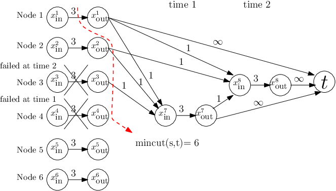

Fig. 8 shows another example that illustrates how choosing the helpers properly can allow for smaller storage and repair-bandwidth. The parameters of the storage network in this figure are . The goal of this example is to store a data object of size such that the network can tolerate failures. Without loss of generality, we assume that node 4 fails in time 1 and the helpers of the newcomer (replacing node 4) are nodes 1, 2, and 3. Now assume that node 3 fails in time 2. We will demonstrate in the following how the helper choice at time 2 (for replacing node 3) will substantially affect the reliability of the distributed storage network.
Choice 1: Suppose the helpers of node 3 in time 2 are nodes 1, 2, and 4. See Fig. 8(a). Now we consider the data collector which would like to reconstruct the original file of size 7 from nodes 1, 3, and 4. By noticing that one of the edge cuts from the virtual source to the data collector has value 6 (see the red dashed curve in Fig. 8(a)), it is thus impossible for the data collector to reconstruct the original file. In fact, we have from Section II-D that, when the newcomer chooses its helpers blindly, to protect a file of size , the minimum repair-bandwidth needed is . Therefore, the repair-bandwidth (our parameter values are ) is not enough to meet the reliability requirement when a BR scheme is used, which agrees with the discussion above.
Choice 2: Suppose the helpers of node 3 in time 2 are nodes 4, 5, and 6. See Fig. 8(b). Now we consider the same data collector that accesses nodes 1, 3, and 4. One can verify that the min-cut value from source to the data collector is 7, which is equal to the target file size 7. Furthermore, one can check the rest different ways of setting up the data collectors and they all have . The above observation illustrates that helper selection choice (Choice 2) can strictly improve the min-cut value of the network.
The choice of the helpers in this example follows the family repair (FR) scheme described in Section IV-B. In Section IV-D, it is proved rigorously that not only we can improve the min-cut value in the end of the first 2 time slots, but the min-cut-value is always even after arbitrarily many failure/repair stages with intelligent helper selection for each time slot. We can thus meet the reliability requirement with intelligent helper selection. This example with parameters is thus another evidence that good helper selection can strictly improve the system performance, i.e., reducing the total repair-bandwidth from (the smallest possible when BR is used) to (since our system has and ).
Appendix B Proof of Proposition 2
Consider any IFG where is a stationary repair scheme. Consider any data collector of and call the set of active output nodes it connects to . Since all the incoming edges of have infinite capacity, we can assume without loss of generality that the minimum cut satisfies and .
Let denote the set of edges in the minimum cut. Let be the chronologically -th output node in , i.e., from the oldest to the youngest. Since , there are at least output nodes in . We now consider the oldest output nodes of , i.e., to . For to , let denote the node index of . Obviously, the vector belongs to .
Consider , we have two cases:
- •
If , then the edge is in .
- •
If , since has an in-degree of and is the oldest node in , all the incoming edges of must be in .
From the above discussion, these edges related to contribute at least a value of to the min-cut value since by definition . Now, consider , we have three cases:
- •
If , then the edge is in .
- •
If and , since one of the incoming edges of can be from , then at least incoming edges of are in .
- •
If and , since no incoming edges of are from , then all incoming edges of are in .
Therefore, these edges related to contribute a value of at least to the min-cut value, where the definition of takes care of the second and the third cases. Consider , we have five cases:
- •
If , then the edge is in .
- •
If and , since one of the incoming edges of can be from , then at least incoming edges of are in . Note that there cannot be an incoming edge of from since only connects to active output nodes at the time of repair and is no longer active since (of the same node index ) has been repaired after .
- •
If ; ; and ; since one of the incoming edges of can be from and another edge can be from , then at least incoming edges of are in .
- •
If and only one of or is in , since one of the incoming edges of is from either or , then at least incoming edges of are in .
- •
If and , then at least incoming edges of are in .
Therefore, these edges related to contribute a value of at least to the min-cut value, where the definition of takes care of the second to the fifth cases.
In the same manner, we can prove that the chronologically -th output node in contributes at least a value of to the min-cut value. If we sum all the contributions of the oldest output nodes of we get (13), a lower bound on the min-cut value.
Appendix C Proof of Inequality (31)
Denote the smallest IFG in by . Specifically, all its nodes are intact, i.e., none of its nodes has failed before. Denote its active nodes arbitrarily by . Consider the family index permutation of the FR scheme that attains the minimization of the right-hand side of (31) and call it . Fail each active node in of exactly once in a way that the sequence of the family indices of the failed nodes is . Along this failing process, we repair the failed nodes according to the FR scheme . For example, let and suppose the minimizing family index permutation is . Then, if we fail nodes 1, 4, 2, 6, 7, 8, 3, and 5 in this sequence, the corresponding family index sequence will be , which matches the given . Note that the node failing sequence is not unique in our construction. For example, if we fail nodes 3, 5, 2, 6, 8, 7, 1, and 4 in this sequence, the corresponding family index vector is still . Any node failing sequence that matches the given will suffice in our construction. We call the resulting new IFG, .
Consider a data collector in that connects to the oldest newcomers. (Recall that in our construction, has exactly newcomers.) Now, by the same arguments as in [4, Lemma 2], we will prove that for the specifically constructed and . Number the storage nodes (input-output pair) of the nodes is connected to by . Define cut between and as the following: for each , if then we include in ; otherwise, we include both and in . It is not hard to see that the cut-value of the cut is equal to .
Appendix D Proof of Inequality (35)
We prove (35) by explicit construction. For any vector , we will use the following procedure, Modify, to gradually modify in 4 major steps until the end result is the desired that satisfies (35). A detailed example illustrating procedure Modify is provided in Appendix E to complement the following algorithmic description of Modify.
Step 1: If there are such that and the -th and the -th coordinates of are equal, i.e., , then we can do the following modification. For convenience, we denote the value of by . Suppose that node belongs to the -th family. We now check whether there is any value satisfying simultaneously (i) ; (ii) node is also in the -th family; and (iii) is not equal to any of the coordinates of . If such exists, we replace the -th coordinate of by . Specifically, after this modification, we will have and .
Repeat this step until either there is no repeated , or until no such can be found.
Step 2: After finishing Step 1, we perform the following modification. If there still are distinct such that and , then we again denote the value of by . Suppose node belongs to the -th family. Consider the following two cases. If the -th family is the incomplete family, then no further modification will be made.
If the -th family is a complete family, then do the following modification.
Find the largest such that node and find the largest such that belongs to the -th family (the same family of node ). If , then we set . If , then we swap the values of and to construct . That is, we first set for all coordinates except for the -th and the -th coordinates, and then set and . After we have constructed new depending on whether or not, we now check whether there is any value satisfying simultaneously (i) node belongs to a complete family (not necessarily the Q-th family); and (ii) is not equal to any of the coordinates of . If such exists, we replace the -th coordinate of by , i.e., set .
Repeat this step until the above process does not change the value of any of the coordinates of .
After finishing the above two steps, the current vector must be in one of the following cases. Case 1: No two coordinates are equal, i.e., for all pairs ; Case 2: there exist a pair such that . We have two sub-cases for Case 2. Case 2.1: All such pairs must satisfy that node belongs to a complete family. Case 2.2: All such pairs must satisfy that node belongs to the incomplete family. Specifically, the above construction (Steps 1 and 2) has eliminated the sub-case that some pair has belonging to a complete family and some other pair has belonging to the incomplete family. The reason is as follows. Suppose some pair has belonging to a complete family. Since we have finished Step 2, it means that any node that belongs to a complete family must appear in one of the coordinates of . Since there are number of nodes belonging to complete families, at least number of coordinates of must refer to a node in a complete family (since and have the same value). Therefore, there are at most number of coordinates of referring to a node in the incomplete family. However, if we have another pair has belonging to the incomplete family, then it means that the coordinates of can refer to at most distinct nodes of the incomplete family (since and are equal). Since there are distinct nodes in the incomplete family, there must exist a value such that node belongs to the incomplete family and does not appear in any one of the coordinates of . This contradicts the fact that we have exhausted Step 1 before moving on to Step 2.
We now consider Cases 1, 2.1, and 2.2, separately. If the vector is in Case 1, then such belongs to and our construction is complete. If belongs to Case 2.2, then do Step 3. If belongs to Case 2.1, do Step 4.
Step 3: We use to denote the pair of values such that and . Denote the value of by . Since we are in Case 2.2, node belongs to the incomplete family. Find the largest such that node and find the largest such that belongs to the incomplete family. If , then we keep as is. If , then we swap the values of and . Recall that we use to denote the family index of the last complete family. We now choose arbitrarily a value from . Namely, is the index of a node of the last complete family. Fix the value. We then replace by the arbitrarily chosen .
If the value of one of the coordinates of (before setting ) is , then after setting we will have some satisfying . In this case, we start over from Step 1. If none of the coordinates of (before setting ) has value , then one can easily see that after setting there exists no satisfying “ belong to a complete family” since we are in Case 2.2 to begin with. In this case, we are thus either in Case 1 or Case 2.2. If the new is now in Case 1, then we stop the modification process. If the new is still in Case 2.2, we will then repeat this step (Step 3).
Step 4: We use to denote the pair of values such that and . Denote the value of by . Since we are in Case 2.1, node belongs to a complete family. Suppose is in the -th complete family. Find the largest such that node and find the largest such that belongs to the -th complete family. If , then we keep as is. If , then we swap the values of and . We now find a value such that (i) node belongs to the incomplete family; and (ii) is not equal to any of the coordinates of . Note that such value always exists. The reason is that since we are now in Case 2.1 and we have finished Step 2, it means that any node that belongs to a complete family must appear in one of the coordinates of . Therefore, there are at least number of coordinates of referring to a node in one of the complete families. This in turn implies that there are at most number of coordinates of referring to a node in the incomplete family. Since there are distinct nodes in the incomplete family, there must exist a value such that node belongs to the incomplete family and does not appear in any one of the coordinates of .
Once the value is found, we replace the -th coordinate of by , i.e., . If the new is now in Case 1, then we stop the modification process. Otherwise, must still be in Case 2.1 since we replace by a that does not appear in before. In this scenario, we will then repeat this step (Step 4).
An example demonstrating the above iterative process is provided in Appendix E.
To prove that this construction is legitimate, we need to prove that the iterative process ends in a finite number of time. To that end, for any vector , define a non-negative function by
One can then notice that in this iterative construction, every time we create a new vector that is different from the input vector , the value of decreases by at least 1. As a result, we cannot repeat this iterative process indefinitely. When the process stops, the final vector must be in Case 1. Therefore, the procedure Modify converts any vector to a new vector such that all coordinate values of are distinct. What remains to be proved is that along the above 4-step procedure, the inequality (35) always holds. That is, the value of is non-increasing along the process. The detailed proof of the non-increasing will be provided shortly. From the above discussion, we have proved (35).
In the rest of this appendix, we prove the correctness of Modify. For each step of Modify, we use to denote the input (original) vector and to denote the output (modified) vector. In what follows, we will prove that the and vectors always satisfy
| (55) |
In Step 1 of the procedure, suppose that we found such . Denote the vector after we replaced the -th coordinate with by . We observe that for , we will have since over and the new belongs to the -th family, the same family as node . For , we will have . The reason is that by our construction, we have . For any , only counts the repeated once. Therefore, will count the same as well. On the other hand, may sometimes be larger than , depending on whether the new or not. The fact that for all to implies (55).
In Step 2, if , then we will not swap the values of and . On the other hand, also means that . In this case, is modified from such that if such a is found. For , since over this range of . We now consider the case of . Suppose node belongs to the -th family. We first notice that by the definition of and the definition of the family repair scheme, is equal to the number of distinct nodes in the -th family that appear in the first coordinates of minus the number of distinct nodes in the -th family that appear in the first coordinates of . For easier reference, we call the former and the latter and we will quantify these two terms separately.
Since we start Step 2 only after Step 1 cannot proceed any further, it implies that all distinct nodes of family must appear in otherwise we should continue Step 1 rather than go to Step 2. Then by our specific construction of , all distinct nodes of family must appear in the first -th coordinates of . Therefore . Since there are exactly distinct nodes in the -th family, by the definition of , we must have . The above arguments show that , which implies the desired inequality when .
We now consider the case when . In this case, we still have . The reason is that by our construction, we have . For any , only counts the repeated once. Therefore, will count the same as well. On the other hand, may sometimes be larger than , depending on whether the new or not. The fact that for all implies (55).
Now, we consider the case when , which implies that and Step 2 swaps the -th and the -th coordinates of . Note that after swapping, we can see that if we apply the same and construction to the new swapped vector, then we will have . By the discussion in the case of , we know that replacing the value of by will not decrease the value for any to and (55) still holds. As a result, we only need to prove that swapping the -th and the -th coordinates of does not decrease the value of .
To that end, we slightly abuse the notation and use to denote the resulting vector after swapping the -th and the -th coordinates of (but before replacing by ). For the case of , we have since for , , and both and are from the same family . For , we have . The reason is as follows. We first observe that . For any , only counts the repeated once (since by our construction of we naturally have ). Therefore, will count the same as well. On the other hand, may sometimes be larger than , depending on whether the new or not. We thus have for .
For the case of , we notice that and are from the same -th family. Therefore, we have . For the case of , we argue that . This is true because of the definition of and the fact that both and . In summary, we have proved for to , which implies (55).
In Step 3, we first consider the case of , which means that is replaced with , a node from the last complete family. For , since we have for all , we must have . We now consider the case of . By the definition of and the definition of the family repair scheme, is equal to the number of distinct nodes in the incomplete family that appear in the first coordinates of minus the number of distinct nodes in the last complete family that simultaneously (i) belong to the helper set of the incomplete family and (ii) appear in the first coordinates of . For easier reference, we call the former and the latter and we will quantify these two terms separately.
Since we have finished executing Step 1, it means that all nodes in the incomplete family appear in the vector . By our construction of , all nodes in the incomplete family must appear in the first coordinates of . Therefore, . Since there are exactly distinct nodes in the last complete family that belong to the helper set of the incomplete family, by the definition of , we must have . The above arguments show that , which implies the desired inequality .
For the case of , we also have . The reason is that by our construction, we have . For any , only counts the repeated once. Therefore, will count the same as well. On the other hand, may sometimes be larger than , depending on whether the new or not. We have thus proved that for all to , which implies (55).
We now consider the case of . Namely, we swap the -th and the -th coordinates of before executing the rest of Step 3. We can use the same arguments as used in proving the swapping step of Step 2 to show that after swapping, we still have for all to , which implies (55). The proof of Step 3 is complete.
In Step 4, we again consider the case of first. In this case, is replaced with , a node of the incomplete family. For , since over this range of . For , we have to consider two cases. If the -th family is the last complete family, then is equal to the number of distinct nodes in the -th family that simultaneously (i) belong to the helper set of the incomplete family and (ii) appear in the first coordinates of , minus the number of distinct nodes in the incomplete family that appear in the first coordinates of . For easier reference, we call the former and the latter . If, however, the -th family is not the last complete family, then is equal to the difference of another two terms. We slightly abuse the notation and refer again to the two terms as and where is the number of distinct nodes in the -th family that appear in the first coordinates of and is the number of distinct nodes in the last complete family that simultaneously (i) does not belong to the helper set of the incomplete family and (ii) appear in the first coordinates of plus the number of distinct nodes in the incomplete family that appear in the first coordinates of .
We will now quantify these two terms separately. Since we have finished executing Step 1 and by the construction of , all nodes in the -th family must appear in the first coordinates of , which are the same as the first coordinates of . Therefore, the value of is if the -th family is the last complete family or if it is one of the first complete families. We now quantify . For when the -th family is the last complete family, since there are exactly distinct nodes in the incomplete family, by the definition of , we must have . When the -th family is not the last complete family, since the number of distinct nodes in the incomplete family is and the number of distinct nodes in the last complete family that do not belong to the helper set of the incomplete family is and their summation is . The above arguments show that for both cases, which implies the desired inequality for .
For , since was a repeated node, then it was already not contributing to for all . Thus, for all to . (Please refer to the case in Step 3 for detailed elaboration.) In summary, after Step 4, assuming , we have for all to , which implies (55).
Finally, we consider the case of . Namely, we swap the -th and the -th coordinates of before executing the rest of Step 4. We can use the same arguments as used in proving the swapping step of Step 2 to show that the inequality (55) holds after swapping. The proof of Step 4 is thus complete.
Appendix E An Illustrative Example for the Modify Procedure
For illustration, we apply the procedure Modify to the following example with and some arbitrary . Recall that family 1 contains nodes , family 2 (last complete family) contains nodes , and the incomplete family, family 0, contains nodes . Suppose the initial vector is . We will use Modify to convert to a vector
We first enter Step 1 of the procedure. We observe1111 11 We also observe that and we can choose and instead. Namely, the choice of is not unique. In Modify, any choice satisfying our algorithmic description will work. that ( and ) and node 2 belongs to the first family. Since node 3 is also in family 1 and it is not present in , we can choose . After replacing by 3, the resulting vector is . Next, we enter Step 1 for the second time. We observe that . Since node 8 is in family 0 and it is not present in , we can choose . The resulting vector is . Next, we enter Step 1 for the third time. For the new , we have and , but for both cases we cannot find the desired value. As a result, we cannot proceed any further by Step 1. For that reason, we enter Step 2.
We observe that for , we find , the last coordinate of equal to , and , the last coordinate of that belongs to family 1. By Step 2, we swap and , and the resultant vector is . Now, since node 5 belongs to family 2, a complete family, and it is not present in , we can choose . After replacing by , the resultant vector is . Next, we enter Step 2 for the second time. Although , we notice that node 7 is in family 0. Therefore, we do nothing in Step 2.
After Step 2, the latest vector is , which belongs to Case 2.2. Consequently, we enter Step 3. In Step 3, we observe that , the last coordinate of being 7, and , the last coordinate of that belongs to the incomplete family, family 0. Thus, we swap and , and the resultant vector is . Now, we choose arbitrarily a value from , the last complete family. Suppose we choose1212 12 We can also choose or . For those choices, the iterative process will continue a bit longer but will terminate eventually. . The resultant vector is . Since we have no other repeated nodes of family 0, the procedure finishes at this point. Indeed, we can see that the final vector , which has no repeated nodes and is the result expected.
Appendix F Proof of Proposition 4
For fixed values, define function as
| (56) |
We first note that by (14), we must have for some integer . The value of depends on the values and the minimizing family index permutation , but does not depend on . We then define as the value such that . We will first prove that by contradiction. Suppose . Since is one way that can satisfy , the minimum-bandwidth consumption must satisfy . Therefore, we must have . However, we then have the following contradiction.
| (57) |
where the first inequality is by knowing that satisfies the reliability requirement; the second inequality is by the definition of ; the first equality is by (14); and the third inequality (the only strict inequality) is by the fact that for all and by the assumption of ; and the last equality is by the construction of .
The above arguments show that . To prove that , we first prove
| (58) |
The reason behind (58) is that (i) and we thus have at least one summand in the RHS of (14); and (ii) the first summand is always since for any family index permutation . Suppose . Obviously, we have by the construction of . Therefore, we must have . However, we then have the following contradiction
| (59) |
where the first inequality is by knowing that satisfies the reliability requirement, the second inequality is by (58), and the equality is by the construction of .
The above arguments prove that . This also implies that when considering the MBR point, instead of finding a that minimizes (14), we can focus on finding a that minimizes
| (60) |
instead, i.e., we remove the minimum operation of (14) and ignore the constant , which does not depend on . We are now set to show that is the minimizing family index permutation at the MBR point.
First, define
| (61) |
Notice that a family index permutation that minimizes also minimizes (60). Therefore, any minimizing family index permutation for (60), call it , must satisfy
| (62) |
Consider the following two cases:
Case 1: , i.e., we do not have an incomplete family.
Consider any family index permutation and let be the number of the first coordinates of that have value . Recall that there is no incomplete family in this case. Suppose the -th coordinate of is . Then, we notice that the expression “” counts the number of appearances of the value in the first coordinates of (recall that there is no incomplete family in this case). Therefore, we can rewrite (61) by
| (63) |
We now prove the following claim.
Claim 6
The above equation implies that a family index permutation is a minimizing permutation if and only if
| (64) |
Proof:
We first prove the only if direction by contradiction. The reason is as follows. If for some , then we consider another family permutation and denote its corresponding values by , such that , , and all other s remain the same. Clearly from (63), such will result in strictly smaller . Note that such with the new , always exists. The reason is the following. By the definition of and the fact that is a family index permutation, we have for all . The inequality then implies and . Therefore, out of the first coordinates of , at least one of them will have value ; and out of the last coordinates of , at least one of them will have value . We can thus swap arbitrarily one of the family indices from the first coordinates with another family index from the last coordinates and the resulting will have the desired and .
We now prove the if direction. To that end, we first observe that the equality always holds because of our construction of . Then (64) implies that we can uniquely decide the distribution of even though we do not know what is the minimizing permutation yet. For example, if , , to satisfy (64), and the summation is , then among , , and , two of them must be 2 and the other one must be 1. On the other hand, we observe that the value of depends only on the distribution of , see (63). As a result, the above arguments prove that any satisfying (64) is a minimizing .
∎
Finally, by the construction of the RFIP , it is easy to verify that the RFIP satisfies (64). Therefore, the RFIP is a minimizing permutation for this case.
Case 2: , i.e., when we do have an incomplete family. In this case, we are again interested in minimizing (60), and equivalently minimizing (61). To that end, we first prove the following claim.
Claim 7
Find the largest such that the -th coordinate of is 0. If no such can be found, we set . Find the smallest such that the -th coordinate of is a negative number if no such can be found, we set . We claim that if we construct and based on a that minimizes , we must have .
Proof:
We prove this claim by contradiction. Consider a minimizing family index permutation and assume . This means, by our construction, that . Since the -th coordinate of is a negative number by construction, counts all coordinates before the -th coordinate of with values in , i.e., it counts all the values before the -th coordinate except for the values and , where is the family index of the last complete family. Thus, knowing that there are no values before the -th coordinate of , we have that
| (65) |
where is the number of values before the -th coordinate. Similarly, since the -th coordinate is 0, we have that counts all coordinates before the -th coordinate of with values in , i.e., it counts all the values before the -th coordinate except for the values and . Thus, we have that
| (66) |
where is the number of 0 values preceding the -th coordinate in and is the number of values preceding the -th coordinate in . Now, swap the -th coordinate and the -th coordinate of , and call the new family index permutation . Specifically, has the same values as on all its coordinates except at the -th coordinate it has the value 0 and at the -th coordinate it has the value . For , we have that since the first coordinates of the two family index permutations are equal. Moreover, since there are no negative values before the -th coordinate of , we have that
| (67) |
where is the number of 0 values in preceding the -th coordinate.
For , if the -th coordinate of is either or , then ; otherwise, . The reason behind this is that the function now has to take into account the new 0 at the -th coordinate when the -th coordinate is either or . When the value of the -th coordinate is in , then by the definition of , we have . The last situation to consider is when the value of the -th coordinate is . In this case, we still have since already does not count the value on the -th coordinate of since it is a negative value.
Denote the number of and values from the -th coordinate to the -th coordinate of by . We have that
| (68) |
since the -th coordinate of has a value. Finally, for , we have that since the order of the values preceding the -th coordinate in a permutation does not matter for . By the above, we can now compute the following difference
| (69) | ||||
| (70) | ||||
| (71) | ||||
| (72) |
where (69) follows from for all and for all ; (70) follows from our analysis about when the -th coordinate of belongs to and otherwise, and there are thus coordinates between the -th coordinate and the -th coordinate of that satisfy ; (71) follows from (65) to (68); and (72) follows from the facts that and that since we have a value at the -th coordinate of . By (72), we have that has a strictly smaller “”. As a result, the case of is impossible.
By the construction of and , it is obvious that . Hence, we must have . The proof of this claim is complete. ∎
Claim 7 provides a necessary condition on a minimizing permutation vector. We thus only need to consider permutations for which . That is, instead of taking the minimum over all , we now take the minimum over only those satisfying .
This observation is critical to our following derivation. The reason is that if we consider a permutation that has , then the expression “” is not equal to the number of appearances of the value in the first coordinates of (recall that by our construction the -th coordinate of is 0). Instead, by the definition of , is the number of appearances of the values 0 and in the first coordinates of . Therefore, we cannot rewrite (61) as (63) if .
On the other hand, Claim 7 implies that we only need to consider those satisfying . We now argue that given any satisfying , for all to , the expression is now representing the number of appearances of and in the first coordinates of , where is the absolute value of the -th coordinate of . The reason is as follows. Let denote the absolute value of the -th coordinate of . If , then by the definition of , we have that represents the number of appearances of in the first coordinates of . If , then by the definition of , we have that represents the number of appearances of 0 and in the first coordinates of . However, by the construction of , we have . Since , we have . This implies that in the first coordinates of , none of them is of value . As a result, we have that again represents the number of appearances of 0 in the first coordinates of .
We now proceed with our analysis while only considering those satisfying as constructed in Claim 7. Let be the number of the first coordinates of that have values or . We can then rewrite (61) by
| (73) |
The above equation implies that a family index permutation is a minimizing permutation if and only if either
| (74) |
or
| (75) |
If we compare (74) and (75) with (64) in Claim 6, we can see that (75) is similar to (64). The reason we need to consider the situation described in (74) is that the range of is from 0 to while the range of all other s is from 0 to . Therefore, we may not be able to make as close to other s (within a distance of 1) as we would have hoped for due to this range discrepancy. For some cases, the largest we can choose is , which gives us the first scenario when all the remaining s are no less than this largest possible value. If can also be made as close to the rest of s, then we have the second scenario.
The proof that (74) and (75) are the if-and-only-if condition on can be completed using the same arguments as in the proof of Claim 6. Finally, notice that the RFIP satisfies (74) or (75) and has . As a result, must be one of the minimizing permutations . The proof of this proposition is hence complete.
Appendix G Proof of Proposition 5
We first consider the case when . We have since otherwise the MSR point cannot satisfy (3) even when plugging in in (14). Define
| (76) |
By (14), we have that the pair
| (77) |
satisfies (3) since . Therefore, is not only a lower bound of but is also achievable, i.e., . Now, for any pair satisfying
| (78) |
for some , we argue that (3) does not hold anymore. The reason is the following. When and , we plug in the vector that maximizes (76) into (14). Therefore, for at least one , we will have . This implies “” when evaluated using . By taking the minimum over all , we still have “”. Therefore, the above choice of cannot meet the reliability requirement at the MSR point. As a result, we have .
We now argue that . According to the definition of function , . Recall that the size of a helper set is , which is strictly larger than . We can thus simply set the values of the first coordinates of to be the family indices of the distinct helpers (out of distinct helpers) of a node and place the family index of this node on the -th coordinate. Such a permutation will have . Therefore, we have proved that .
We now consider the remaining case in which . To that end, we first notice that for any values we have number of complete families. Also recall that family 1 is a complete family and all families are the helpers of family 1, and there are thus number of nodes in total of family index . We now consider a permutation in which all its first coordinates are family indices not equal to 1 and its last coordinates are of family index 1. Observe that if we evaluate the objective function of the right-hand side of (14) using , out of the summands, of to , we will have exactly non-zero terms since (i) by the definition of , we always have and therefore, when , we always have ; (ii) whenever , the corresponding term due to the special construction of the . As a result, when a sufficiently large is used, we have
| (79) |
The above equality implies . Otherwise if , then we will have “” when using the aforementioned , which implies that “” holds still when minimizing over all . This contradicts the definition that and satisfy the reliability requirement.
On the other hand, we know that and for the BR scheme when , see (7). Since the performance of the FR scheme is not worse than that of the BR scheme, we have and for the FR scheme. Hence, the proof is complete.
Appendix H Proof of Corollary 3
First consider the case when . Since there are number of families (complete plus incomplete families) and , any family index permutation has at least one pair of indices of the same family in its first coordinates. Using (14), this observation implies that
| (80) |
Now define as a family index permutation such that its first coordinates, in this order, are if and define as if . Since all the coordinates have different values except the first coordinate and the -th coordinate have equal value , and since they have no value, we have
| (81) |
Thus, we get the equality in (37).
We now consider the case when . Before proceeding, we first argue that among all values satisfying (1), the only possible cases of having are either or . The reason behind this is the following. Suppose . For any , we have
| (82) | ||||
| (83) |
where we get (82) by our assumption that and (83) follows from the assumption that . The above contradiction implies either or . Since Corollary 3 requires , the only remaining possibility is . However, will not have a valid value since in this case we have , which implies , an impossible paramemter value violating (1). Hence, the proof is complete.
Appendix I Proof of Corollary 2
Consider first the case when . Without loss of generality, assume that and for to , i.e., the indices to correspond to the regular groups and the index corresponds to the remaining group. Now, applying the same reasoning as in the proof of Proposition 4 to (23), we have that for the family-plus repair scheme as well. In the following, we will prove that (i) if , then one minimizing vector can be constructed by setting for to and ; (ii) if , then we can construct a minimizing vector by setting and among all to , at most one satisfies .
To prove this claim, we first notice that since we are focusing on the MBR point, we can assume is sufficiently large. Therefore, we can replace the minimizing permutation for each summand of (23) by the RFIP (of for the summand to and of for summand ) using the arguments in the proof of Proposition 4. Therefore, we can rewrite (23) by
| (84) |
where is the RFIP of for to and the RFIP of for . Note that for , in the FR scheme we have 2 complete families and no incomplete family and the RFIP in this case is . As a result, for all to . For , we have one complete family and one incomplete family and the RFIP in this case is
| (85) |
We thus have . We now argue that a vector satisfying conditions (i) and (ii) stated above minimizes (84). Note first that both and are non-decreasing with respect to according to our construction of the RFIP. Also, we always have for all .
We are now ready to discuss the structure of the optimal vector. Since for each to , we are summing up the first from to and in total there are such terms, (84) implies that to minimize (23) we would like to have as many terms corresponding to “large ” as possible in the summation terms. If , this can be done if and only if we set all to 0 except for one value to be , which is our construction (i). If , this can be done if and only if we set and, for to , we set all to either or except for one .
Knowing that is of this special form, we can compute the RHS of (23) by
| RHS of (23) | ||||
| (86) |
where is the number of from 1 to with in the minimizing vector ; is the contribution to the min-cut value from those groups with , which is equal to ; is the contribution to the min-cut value from the single regular group with , which is equal to ; and is the contribution to the min-cut value from the remaining group (group ), which is equal to
| (87) |
By plugging in the expressions of the RFIPs and , we have
| (88) |
where and (88) follows from the fact that when and . The minimum repair-bandwidth thus satisfies (24).
Now, for the case when , in a similar fashion, we can prove that a vector minimizes the right-hand side of (23) at the MBR point if and only if there is at most one such that . By setting for all in (84), recall that is the RFIP for , we get
| RHS of (23) | (89) |
and thus satisfies (24) for this case too. The proof is hence complete.
Appendix J Proof of Proposition 9
We first show that whenever , we have
| (90) |
where is the collection of IFGs of an FR scheme . That is, when , the additional step of partitioning nodes into sub-groups in the family-plus scheme will monotonically improve the performance when compared to the original FR scheme without partitioning.
When , the family-plus repair scheme collapses to the FR scheme since each group of the family-plus scheme needs to have at least nodes and when we can have at most 1 group. Thus, trivially, we have (90) when . Now, we consider the case when .
We first consider the original FR scheme (the RHS of (90)). In this case, the FR scheme has complete family and one incomplete family. The corresponding RFIP is thus
By Proposition 4, we have
| (91) |
where (91) from the fact that when .
We now turn our focus to the family-plus repair scheme. Consider first the case when . If , we have by (24) and (91) that (90) is true since the third term on the LHS of (24) is the RHS of (91). If , we again have by (24) and (91) that (90) is true since the second term on the LHS of (24) is no less than the RHS of (91). Now, consider the case when . Similarly, we have by (24) and (91) that (90) is true since the first term on the LHS of (24) is the RHS of (91).
We are now ready to prove (25). If neither (i) nor (ii) of Proposition 1 is true, we must have one of the three cases: (a) and ; (b) , , and even ; and (c) , , and odd . For case (a), since whenever (see the proof of Corollary 3 in Appendix H), we have that . Considering the FR scheme, we thus have that among the first indices of a family index permutation there is at least one family index that is repeated. Jointly, this observation, Proposition 3, the MBR point formula in (15), and (90) imply (25) when . Note that is not possible in case (a) since we will have , which violates (1). For both cases (b) and (c), since by (1), we have . The construction of the family-plus scheme thus will generate at least 2 groups. That is, the value of in Proposition 8 must satisfy . Moreover, in case (b), we have no remaining group since is even. Therefore, since , for any defined in Proposition 8, there are at least two distinct values with . In case (c), we have (note that since we have that by construction). Therefore, similarly, for any defined in Proposition 8, there are at least two distinct values with .
Using the above observation (at least two distinct values having ) and Proposition 8, we have that in both cases (b) and (c)
| (92) |
where the first inequality follows from (i) considering only those values with ; (ii) plugging in the min-cut formula in Proposition 3; and (iii) only counting the first term “” when summing up for all to . The second inequality follows from the assumption that in both cases (b) and (c) and the fact that both and must be strictly positive. By noticing that for cases (b) and (c) the RHS of (25) is indeed , the proof is complete.
Appendix K Proof of Lemma 2

To prove this lemma, we model the problem using a finite directed acyclic graph and then we invoke the results from random linear network coding [8]. The graph has a single source vertex that is incident to other vertices with edges of capacity 1. We call these vertices level 1 vertices. Among these level 1 vertices, we form disjoint groups and each group consists of arbitrarily chosen distinct vertices. The idea is that each group of them is associated with a vertex in . Note that there are vertices forming groups while there are still vertices that do not form any group at all. See Fig. 9 for illustration.
Now, in addition to the source and the level 1 vertices, we add new node pairs for all . Each is connected by an edge of capacity 1. We call the nodes, level 2 vertices and the nodes level 3 vertices. We partition the new node pairs (edges) into groups and each group consists of edges. We then associate each group of edges to one group of level 1 vertices created previously. See Fig. 9 for illustration. Finally, for the level 1, level 2, and level 3 vertices belonging to the same group (there are groups in total), we connect all the level 1 vertices in this group and all the level 2 vertices in this group by an edge with infinite capacity.
We now describe the relationship of the newly constructed graph in Fig. 9 to the graph representation of the generalized fractional repetition code. For easier reference, we use “the graph in Fig. 9” to refer to the newly constructed graph; and use “the graph in Fig. 7” to refer to the graph representation of the generalized fractional repetition codes. There are groups in the graph of Fig. 9 and each group corresponds to one node in of the graph of Fig. 7. We notice that there are number of level 1 vertices in the graph of Fig. 9 and number of edges in of the graph of Fig. 7. As a result, we map each level 1 vertex bijectively to an edge in . There are number of level 3 vertices in the graph of Fig. 9 and there are number of edges in the graph of Fig. 7. As a result, we map each level 3 vertex bijectively to an edge in .
We now focus on the graph of Fig. 9. Assume that source has a file of packets. We perform random linear network coding (RLNC) [8] on the graph of Fig. 9 assuming a sufficiently large finite field is used. After we have finished the RLNC-based code construction on the graph of Fig. 9, we now describe how to map the construction back to the edges in the graph of Fig. 7. Specifically, the coded packet corresponding to where is a level 1 vertex in the graph of Fig. 9 is assigned to the edge (in the graph of Fig. 7) corresponding to node . We now consider the coded packets corresponding to where is a level 2 vertex and is a level 3 vertex in the graph of Fig. 9. Without loss of generality, we assume that belongs to the -th group in Fig. 9 and is the -th level 3 vertex in this group. Then, we assign the coded packets on the edge to the edge (in the graph of Fig. 7) that connects the -th node in and the -th node in .
In the following, we will prove that the above code construction (from the RLNC-based code in the graph of Fig. 9 to the generalized fractional repetition codes in the graph of Fig. 7) satisfies Lemma 2.
To prove that the above construction satisfies Property 1, we notice that any coded packet corresponding to some in the graph of Fig. 7 is now mapped from a edge in Fig. 9 where is a level 2 vertex; is a level 3 vertex; belongs to the -th group in Fig. 9; and is the -th level 3 vertex in this group. By the graph construction in Fig. 9, such a coded packet is a linear combination of the coded packets in Fig. 9 from source to vertex where the vertices are the level 1 vertices corresponding to the -th group. Since those packets along are the packets for all satisfying in the graph of Fig. 7, we have thus proved Property 1: Namely, any coded packet corresponding to some is a linear combination of the packets for all satisfying .
To prove that the above construction satisfies Property 2, for any subset of edges in the graph of Fig. 7, we place a sink node in the graph of Fig. 9 that connects to the corresponding set of level 1/level 3 vertices in Fig. 9 using edges of infinite capacity. See Fig. 9 for illustration of one such . One can quickly verify that the min-cut-value from the source to the sink in the graph of Fig. 9 is the value computed from the given subset of edges in the graph of Fig. 7. As a result, with a sufficiently large finite field , any sink satisfying can successfully reconstruct the original file with close-to-one probability. Since the sink accesses only level 1 and level 3 vertices, the packets in the graph of Fig. 7 that correspond to the level 1 vertices in the graph of Fig. 9 and the packets in the graph of Fig. 7 that correspond to the level 3 vertices in the graph of Fig. 9 jointly can reconstruct the original file of size . Property 2 is thus also satisfied.
By the above arguments, the proof of Lemma 2 is complete.
References
- [1] R. Ahlswede, N. Cai, S.-Y. R. Li, and R. W. Yeung, “Network information flow,” IEEE Trans. Inf. Theory, vol. 46, no. 4, pp. 1204–1216, 2000.
- [2] R. Bhagwan, K. Tati, Y. C. Cheng, S. Savage, and G. M. Voelker, “Total recall: System support for automated availability management,” in Proc. 1st Conf. on Networked Systems Design and Implementation (NSDI), San Francisco, CA, Mar. 2004, pp. 25–25.
- [3] V. R. Cadambe, S. A. Jafar, H. Maleki, K. Ramchandran, and C. Suh, “Asymptotic interference alignment for optimal repair of mds codes in distributed storage,” IEEE Trans. Inf. Theory, vol. 59, no. 5, pp. 2974–2987, 2013.
- [4] A. G. Dimakis, P. B. Godfrey, Y. Wu, M. J. Wainwright, and K. Ramchandran, “Network coding for distributed storage systems,” IEEE Trans. Inf. Theory, vol. 56, no. 9, pp. 4539–4551, 2010.
- [5] S. El Rouayheb and k. Ramchandran, “Fractional repetition codes for repair in distributed storage systems,” in Proc. 48th Annual Allerton Conf. on Comm., Contr., and Computing., Monticello, Illinois, Sept. 2010, pp. 1510–1517.
- [6] S. Ghemawat, H. Gobioff, and S. T. Leung, “The google file system,” in Proc. 19th ACM Symp. on Operating Systems Principles (SOSP), Bolton Landing, NY, Oct. 2003, pp. 29–43.
- [7] P. Gopalan, C. Huang, H. Simitci, and S. Yekhanin, “On the locality of codeword symbols,” IEEE Trans. Inf. Theory, vol. 58, no. 11, pp. 6925–6934, 2012.
- [8] T. Ho, M. Médard, R. Koetter, D. R. Karger, M. Effros, J. Shi, and B. Leong, “A random linear network coding approach to multicast,” IEEE Trans. Inf. Theory, vol. 52, no. 10, pp. 4413–4430, 2006.
- [9] H. D. L. Hollmann, “On the minimum storage overhead of distributed storage codes with a given repair locality,” in Proc. IEEE Int. Symp. Information Theory (ISIT), Honolulu, HI, Jun. 2014, pp. 1041–1045.
- [10] G. M. Kamath, N. Prakash, V. Lalitha, and P. V. Kumar, “Codes with local regeneration,” in IEEE Information Theory and Applications Workshop (ITA), San Diego, CA, Feb. 2013, pp. 1–5.
- [11] G. M. Kamath, N. Silberstein, N. Prakash, A. S. Rawat, V. Lalitha, O. O. Koyluoglu, P. Kumar, and S. Vishwanath, “Explicit mbr all-symbol locality codes,” in Proc. IEEE Int. Symp. Information Theory (ISIT), Istanbul, Turkey, Jul. 2013, pp. 504–508.
- [12] D. S. Papailiopoulos and A. G. Dimakis, “Locally repairable codes,” in Proc. IEEE Int. Symp. Information Theory (ISIT), Cambridge, MA, Jul. 2012, pp. 2771–2775.
- [13] D. S. Papailiopoulos, J. Luo, A. G. Dimakis, C. Huang, and J. Li, “Simple regenerating codes: Network coding for cloud storage,” in Proc. IEEE INFOCOM, Orlando, FL, Mar. 2012, pp. 2801–2805.
- [14] N. Prakash, G. M. Kamath, V. Lalitha, and P. V. Kumar, “Optimal linear codes with a local-error-correction property,” in Proc. IEEE Int. Symp. Information Theory (ISIT), Cambridge, MA, Jul. 2012, pp. 2776–2780.
- [15] K. V. Rashmi, N. B. Shah, and P. V. Kumar, “Optimal exact-regenerating codes for distributed storage at the msr and mbr points via a product-matrix construction,” IEEE Trans. Inf. Theory, vol. 57, no. 8, pp. 5227–5239, 2011.
- [16] K. V. Rashmi, N. B. Shah, P. V. Kumar, and K. Ramchandran, “Explicit construction of optimal exact regenerating codes for distributed storage,” in Proc. 47th Annu. Allerton Conf. Communication, Control, and Computing, Urbana-Champaign,IL, Sep. 2009, pp. 1243–1249.
- [17] A. S. Rawat, O. O. Koyluoglu, N. Silberstein, and S. Vishwanath, “Optimal locally repairable and secure codes for distributed storage systems,” IEEE Trans. Inf. Theory, vol. 60, no. 1, pp. 212–236, 2012.
- [18] S. Rhea, C. Wellis, P. Eaton, D. Geels, B. Zhao, H. Weatherspoon, and J. Kubiatowicz, “Maintenance-free global data storage,” Internet Computing, IEEE, vol. 5, no. 5, pp. 40–49, 2001.
- [19] N. B. Shah, K. V. Rashmi, P. V. Kumar, and K. Ramchandran, “Distributed storage codes with repair-by-transfer and nonachievability of interior points on the storage-bandwidth tradeoff,” IEEE Trans. Inf. Theory, vol. 58, no. 3, pp. 1837–1852, 2012.
- [20] ——, “Interference alignment in regenerating codes for distributed storage: Necessity and code constructions,” IEEE Trans. Inf. Theory, vol. 58, no. 4, pp. 2134–2158, 2012.
- [21] K. W. Shum and Y. Hu, “Cooperative regenerating codes,” IEEE Trans. Inf. Theory, vol. 59, no. 11, pp. 7229–7258, 2013.
- [22] D. B. West, Introduction to graph theory. Prentice Hall Upper Saddle River, NJ., 2001, vol. 2.
- [23] Y. Wu, “Existence and construction of capacity-achieving network codes for distributed storage,” IEEE J. Select. Areas Commun., vol. 28, no. 2, pp. 277–288, 2010.
- [24] Y. Wu and A. G. Dimakis, “Reducing repair traffic for erasure coding-based storage via interference alignment,” in Proc. IEEE Int. Symp. Information Theory (ISIT), Seoul, South Korea, Jul. 2009, pp. 2276–2280.