Detection and Decoding for 2D Magnetic Recording Channels with 2D Intersymbol Interference
Abstract
This paper considers iterative detection and decoding on the concatenated communication channel consisting of a two-dimensional magnetic recording (TDMR) channel modeled by the four-grain rectangular discrete grain model (DGM) proposed by Kavcic et. al., followed by a two-dimensional intersymbol interference (2D-ISI) channel modeled by linear convolution of the DGM model’s output with a finite-extent 2D blurring mask followed by addition of white Gaussian noise. An iterative detection and decoding scheme combines TDMR detection, 2D-ISI detection, and soft-in/soft-out (SISO) channel decoding in a structure with two iteration loops. In the first loop, the 2D-ISI channel detector exchanges log-likelihood ratios (LLRs) with the TDMR detector. In the second loop, the TDMR detector exchanges LLRs with a serially concatenated convolutional code (SCCC) decoder. Simulation results for the concatenated TDMR and averaging mask ISI channel with 10 dB SNR show that densities of 0.48 user bits per grain and above can be achieved, corresponding to an areal density of about 9.6 Terabits/, over the entire range of grain probabilities in the TDMR model.
Index Terms:
Two-dimensional magnetic recording, iterative detection and decoding, rectangular grain model, two-dimensional intersymbol interferenceI Introduction
Industry is approaching the data storage density limit of magnetic disk drives that write data on one-dimensional tracks. Alternative technologies such as heat-assisted-magnetic-recording (HAMR) and bit patterned media recording (BPM) are under active investigation. One drawback of most of these techniques is that they require a radical redesign of the recording medium [1]. Moreover, it is uncertain whether they will come on line quickly enough to prevent a plateau in magnetic disk storage density in the near to medium term.
This paper considers detection and coding techniques for an alternate approach proposed in [1] called two-dimensional magnetic recording (TDMR), wherein bits are read and written in two dimensions on conventional magnetic hard disks. These disks have magnetic grains of different sizes packed randomly onto the disk surface. In TDMR, information bits are channel coded to a density of up to two bits per magnetic grain, and written by a special shingled write process that enables high density recording. A key problem is that a given magnetic grain retains the polarization of the last bit written on it. Hence, if a grain is large enough to contain two bit centers, the older bits will be overwritten by the latest one.
A relatively simple 2D TDMR channel model is the four-grain rectangular discrete-grain model (DGM) introduced in [2], wherein four different grain types are constructed from one, two, or four small square tiles. In [2], upper and lower bounds for the channel capacity of this model are derived showing a potential density of 0.6 user bits per grain. For a typical media grain density of 20 Teragrains/, this corresponds to about 12 Terabits/. This is more than an order of magnitude improvement over current hard disk drives, which exceed densities of 500 Gigabits/ [3].
Coding and detection for the four-grain DGM is considered in a previous paper by Pan, Ryan, et. al. [3]. They construct a BCJR [4] detection algorithm that scans the input image one row (track) at a time. A 16-state trellis is constructed as the Cartesian product of media states (that capture transitions between different grain geometries during a one tile move along a row) and data states (that capture the grain overwrite effect). It is shown that the number of states can be reduced to six by combining equivalent states. After one forward-backward pass through each row of the input image, the TDMR detector passes soft information in the form of log-likelihood ratios (LLRs) to a rate 1/4 serially concatenated convolutional code (SCCC) with puncturing, which decodes the data at the highest rate that achieves a BER of (corresponding to the highest possible user bit density). No iteration between the TDMR detector and SCCC is done in [3], although the possibility is mentioned.
A two-row BCJR detector for the four-grain TDMR channel model has been proposed recently [5]. It considers the outputs of two rows and two columns resulting from bits written on three input rows. Moreover, soft decision feedback of grain state information from previously processed rows is used to aid the estimation of bits on current rows. Finally, the TDMR detector and SCCC decoder iteratively exchange LLRs before a final estimate of the bits is obtained. This two-row BCJR detector increases the code rate by up to 12% over [3].
This paper considers iterative detection and decoding on the concatenated communication channel consisting of the four-grain DGM (TDMR channel) model, followed by a 2D-ISI channel modeled by linear convolution of the DGM model’s output with a finite-extent 2D blurring mask followed by additive white Gaussian noise (AWGN). We propose an iterative detection and decoding scheme that combines TDMR detection, 2D-ISI detection, and soft-in/soft-out (SISO) channel decoding in a structure with two iteration loops. The 2D-ISI detector is based on prior work by the last three authors [6, 7].
The novel contributions of this paper are as follows:
(1) Simulation of the complete two-dimensional magnetic read-write channel,
incorporating the error correction coding, grain over-write effects, and
2D-ISI;
(2) A novel iterative scheme consisting of a double loop structure with
exchange of soft information between the constituent blocks based on the
“turbo principle;”
(3) System parameter optimization using an EXIT chart technique [8];
(4) For the concatenated TDMR and averaging mask ISI channel
with an SNR of 10 dB (respectively 9 dB), the channel coding rate (which is
one half of the user bit density in the modeled scenario) required to
achieve a BER of is shown to be, on average, only
about 7% (respectively 10%) lower than the rate on the TDMR channel alone,
for all values of the probability of two-bit grains considered. For
the 10 dB SNR case, densities of 0.48 user bits per
grain and above can be achieved, corresponding to an areal density of about
9.6 Terabits/.
This paper is organized as follows. Section II summarizes the four grain DGM. Section III provides an overview of the system architecture, explaining the double loop structure. Optimization of system parameters using EXIT chart techniques is presented in section IV. Section V provides simulation results, and section VI concludes the paper.
II System Model
Figure 1 shows a block diagram of the write process (transmission model).

A block of user information bits, denoted as in the block diagram, is encoded by a rate 1/4 SCCC consisting of an eight state rate 1/2 outer non-recursive convolutional code (NRCC) with generator matrix , followed by an interleaver , followed by an inner eight state recursive systematic convolutional code (RCC) with generator matrix , followed by a second interleaver . Code rates greater than (respectively, less than) 1/4 are achieved by puncturing (respectively, repeating) randomly selected output bits from the inner encoder. To compare with the result of [3], the SCCC code in this paper is identical to the one in [3]. See [3, 5] for more details about the SCCC encoder and decoder.
The code word bits are level shifted so that , and then are interleaved again to remove the dependency between code word bits, and then are written onto the TDMR channel with over-write property. The TDMR corrupted block of bits is denoted as , with .
The TDMR channel consists of a rectangular array (image) of unit-sized pixels, where one coded bit is written on each pixel. The image is a (random) combination of four distinct types of rectangular grains. Relative to the unit size their sizes are , , and as shown in Fig. 2.

The four grain types occur with probabilities , , , and , respectively. We assume that the average number of coded bits per grain is 2, i.e. . We also assume that the TDMR channel satisfies an isotropy condition so that type 2 and type 3 grains are equally likely, i.e., . Based on the above assumptions, all of the four probabilities can be computed for a given value of . To model the write process, the TDMR image pixels are given the values (equiprobable) as coded bits in a row-by-row raster scan order. The multi-bit grains can have only one polarity which is determined by the sign of the last bit written on them. This property is known as the over-write property of TDMR channel.

The quadrant notation is defined as follows:
| (1) |
In (1), the grain labels A-I refer to Fig. 2. Using the quadrant notation, we can write the relation between and the relevant interleaved coded bit as follows:
| (2) |
which models the over-write property by imposing an appropriate spatial shift.
Finally, the cross-track and down-track reading process will introduce 2D intersymbol interference (ISI). The TDMR channel with arbitrary 2D-ISI can be modeled as follows [2]:
| (3) |
where h is a 2D read-head impulse response, w is the discrete AWGN field, and y is the actual bits on the magnetic grains as given by (2). In this paper, we consider the case in which the 2D ISI mask h is a averaging mask; i.e., for and , and 0 elsewhere. This means the current pixel receives adjacent-pixel interference with the same magnitude as the current bit, making this h one of the most difficult masks to equalize. Since the mask h operates on each unit pixel value , and the are correlated by the TDMR write model, (2) and (3) incorporate a simple model of grain- and data-dependent 2D-ISI.
III Combined Detector and Decoder
Figure 4 depicts the overall block diagram of the read process (receiver).

The receiver consists of two loops: the loop between 2D-ISI equalizer and TDMR detector and the loop between TDMR detector and SCCC channel decoder. These loops are sometimes referred to as “outer loops.” Note that the SCCC decoder itself consists of a pair of modules corresponding to the constituent encoders described in section II. Iterations between these decoders within the SCCC decoder are referred to as “inner loops.”
The received image is first sent into the 2D-ISI equalizer to mitigate the effect of 2D-ISI and additive noise and obtain an estimate of the TDMR bits . The row-column equalization algorithm using joint extrinsic information proposed in [6] is employed here. This equalizer produces soft-output for a block of pixels, resulting in 16 probabilities for the 16 possible configurations. These probabilities are often represented in the log-domain as LLRs. The output LLR from the 2D-ISI equalizer is defined as follows:
| (5) |
where ranges over the 16 configurations of images located at position . Note that since we serially process the image in a row-by-row order, the row position is fixed and the index merely represents the column position on that row.
The 2D-ISI equalizer output is processed by the TDMR detector’s BCJR algorithm, as described in [5]. The TDMR detector estimates LLRs for coded bits which are deinterleaved and sent to the SCCC decoder, after subtraction of previous input LLRs received from the SCCC. The SCCC decoder computes LLR estimates of , which are interleaved and fed back to the TDMR detector, after subtraction of SCCC input LLRs. This loop is repeated several times, and then the TDMR detector estimates LLRs for which are sent back to the 2D-ISI equalizer. The whole process is repeated until the SCCC decoding converges.
In the following, we describe some details about interfacing the 2D-ISI equalizer with the TDMR detector and the SCCC decoder.

The row detector scans the image in a row-by-row order, whereas the column detector scans it column-by-column. In the row/column equalizer, for a given image position, the current pixel is denoted as . The current state consists of two pixels denoted and and the input consists of two pixels denoted and . The previous state consists of the pixels denoted and . The block of pixels are estimates passed on by the TDMR detector and serve as extrinsic information for the inputs in the row/column equalizer. The pixels denoted and are feedback pixels from previous scan direction (e.g., column direction for row detector). Specifically, in the 2D-ISI BCJR algorithm the computation is implemented as follows:
| (6) |
In (6), the factor is either 0 or 1 based on trellis structure, and is a constant for all valid state transitions (and zero otherwise). is the extrinsic feedback probability from the other (row or column) detector. is the 16-valued feedback probability from the TDMR detector. Since the same vectors are used in both row and column detector, marginalization is needed in each equalizer. For example, as shown in Fig. 5, to compute the a priori joint input probability for the row equalizer, we need to marginalize the over the two state bits and . Similar marginalization is done for the extrinsic probabilities . Based on the analysis in [7], there is no need to subtract the input 16-valued LLRs from the output 16-valued LLRs when exchanging LLRs between row and column equalizers.
Details of the TDMR detector (without 2D-ISI) based on the BCJR algorithm are described in [5]. Here we describe a slight modification of the algorithm to interface the TDMR detector with the 2D-ISI equalizer. In particular, the gamma computation of the BCJR algorithm in the TDMR detector is implemented as follows:
| (7) |
where the term is equal to 1/4, since the two coded bits in the input vector are assumed to be independent of each other and of the grain states. The term is the state transition probability computed from the grain connectivity table in [5]. The summation in the right-hand-side computes a weighted sum of the conditional probabilities in the original BCJR algorithm in [5] with extrinsic probabilities from the 2D-ISI equalizer. The last two factors in (7) are probabilities of the bits in input vector computed from single valued LLRs from the SCCC decoder; they are computed as:
where .
The TDMR detector’s and probabilities are updated as in [4], using the probabilities in (7). Then the joint state and input probabilities at the th step are computed as
| (8) |
The LLRs sent from the TDMR detector to the SCCC decoder are given by
| (9) |
where and . The feedback probabilities sent from the TDMR detector to the 2D-ISI equalizer are computed as
| (10) |
where the probability is defined in (8), and is used to weight the conditional probability when computing the probabilities for the vector . The LLRs sent to the 2D-ISI equalizer are given by
| (11) |
Because the extrinsic probability from the 2D-ISI to the TDMR detector is part of a weighted sum in the TDMR probability (7), it cannot be factored out of the TDMR probability (8), and thus cannot form a separate term in the final LLR. Hence, we do not subtract the incoming 2D-ISI extrinsic information from the TDMR output LLRs in (11) before sending them to the 2D-ISI equalizer. Similarly, the marginalization of the incoming probabilities from the TDMR in (6) makes it impossible to retain these probabilities as multiplicative factors in the final probabilities, making it inadvisable to perform LLR subtraction before sending the 2D-ISI output LLRs to the TDMR detector.
To compensate for the lack of LLR subtraction in the 2D-ISI/TDMR loop, a multiplicative weight factor is applied to LLRs sent to the TDMR detector. This factor reduces the LLR magnitudes passed into the TDMR detector and helps correct pixels that are incorrectly estimated by the 2D-ISI equalizer, which have LLRs of large magnitude but with incorrect sign. For example, Fig. 6 shows the histogram of output conditional LLRs of TDMR detector for the pixels corresponding to codeword bits, before weight is applied, whereas Fig. 7 shows the same LLRs after weighting. A positive LLR means the sign of original bit written on that pixel is successfully recovered by TDMR detector, whereas a negative LLR means that the result on that pixel remains incorrect. The weighting decreases large magnitude wrong LLRs as shown in the zoomed graph, which helps the SCCC decoder to correct the TDMR corrupted codeword. The details of weight selection are described in the following section.


IV Optimization using EXIT Chart
Proper design of the combined read process requires, among other things, specification of the weight mentioned in section III, as well as the iteration schedule—how many inner loops of the SCCC decoder for each outer loop between TDMR detector/SCCC decoder and 2D-ISI equalizer/TDMR detector. This is a multi-parameter optimization problem; brute force search for an optimal choice of parameters by simulation of the complete system can be computationally expensive.
This section describes the EXIT chart method to optimize the weight as well as the iteration schedule. EXIT charts were introduced by ten Brink [8]. They allow the performance of a system of concatenated detectors to be predicted based on input/output mutual information curves for individual constituent detectors, which can be computed relatively quickly. The mutual information between the input extrinsic information LLR to a given detector and the input codeword is computed; similarly the output mutual information between the output extrinsic information LLR from a given detector and the input codeword is computed. The mutual information and are defined as follows:
| (12) |
where is the experimental conditional PDF for input/output LLRs. The EXIT chart is obtained by plotting as a function of for both TDMR detector and SCCC decoder on the same set of axes, using the horizontal axis as for TDMR detector and the vertical axis as for SCCC decoder. Thus a pair of vs curves are obtained for different values of the parameter to be optimized (e.g., weight ). The optimal value of the parameter is one that results in the corresponding pair of vs curves being close to each other, without touching or intersecting. In this paper, we did not jointly optimize the weight and the iteration schedule. Instead, we optimized the weight parameter first, for a fixed iteration schedule. Next, we fixed the weight found in the first step and optimized the iteration schedule.
For EXIT chart optimization, the goal is to select a set of parameter values that results in vs curves satisfying the requirement of not touching with the highest code rate. The EXIT chart optimization in this section is based on the grain image with . In actual experiments, we noticed that the input mutual information varies over only a small range of values. This makes it difficult to generate a complete set of EXIT chart curves. To ameliorate this problem, we simulate input LLRs using a random number generator, whose distribution is close to that of the observed histogram of the input LLR. The random numbers are then injected into TDMR detector as shown in Fig. 8.

Experimentally, we observed that the general extreme value (GEV) distribution was a good fit to the observed TDMR LLR histogram. The probability density function of the GEV distribution is given by
| (13) |
Fig. 9 shows the fit of the GEV distribution to a typical experimental TDMR LLR histogram.

The input mutual information can now be varied by appropriately changing the parameters of GEV. Based on experimental LLR histograms, the parameter of the GEV distribution varies very little when the weight or iteration schedule varies. Therefore we fixed the parameter value of —based on experiments—in our random number generator. The parameters and we observed to satisfy (approximately) the linear relation . However, we set an upper limit for the parameter (4.37 in our experiments) so that the width of the GEV distribution does not grow too large; i.e., we set and vary to simulate different input mutual information values to generate the vs curves. Fig. 10 depicts these curves for different values of the weight . Two inner loops of the SCCC decoder were used for this part of the experiment.

The EXIT chart curves for different weights are fairly close to each other. We numerically computed the distance between pairs of vs curves to determine the weight that yields the maximum distance. Typically, the experimental SCCC input mutual information never rises much higher than 0.4. Therefore, we used the distance between the second points on the two curves as the distance metric. (Out of 13 points on each curve, the second point always has SCCC .) Based on this metric, we determined that the weight results in the farthest apart pair of vs curves.
Next, we fixed the weight and obtained a set of EXIT chart curves by varying the iteration schedule—number of inner loops in the SCCC decoder. Again, we numerically computed the distance between pairs of vs curves to find the iteration schedule that yields the maximum distance. Based on this metric, we determined that ten inner loops of the SCCC decoder gives the farthest apart pair of vs curves.
V Simulation Results
This section presents Monte Carlo simulation results for the system described in section III, and compares its performance to previously published results by Pan and Ryan et. al. [3]. As discussed in section IV, we set the weight , and run ten inner loops of the SCCC decoder for each outer loop of the TDMR detector/SCCC decoder. Three iterations of row/column 2D-ISI equalizer loop and six iterations of the TDMR detector/SCCC decoder loop are done for each iteration of the 2D-ISI equalizer/TDMR detector loop; this outer loop schedule was optimized by multiple simulation runs.
The simulations employ multiple TDMR images; each image is written by the SCCC codeword corresponding to 32,768 randomly generated equiprobable information bits. The encoder described in section II is used. The coded bits are arranged into a rectangular image with 512 columns. The number of rows depends on the total number of codeword bits, which depends on the code rate. A nominal code rate of 1/4 gives 256 rows. The code rate is adjusted by suitable puncturing or repetition of the coded bits. 2D-ISI with the averaging mask and AWGN is imposed on the image as described in section II. The simulations are performed for two different SNR values of 9 dB and 10 dB, computed as in (4). For each value of the grain probability , we adjust the code rate to achieve a decoded BER of . This is ensured by decoding at least 100 codeword blocks of 32,768 information bits each, with at most 32 errors. The maximum code rate achieving this BER is recorded for each value of .
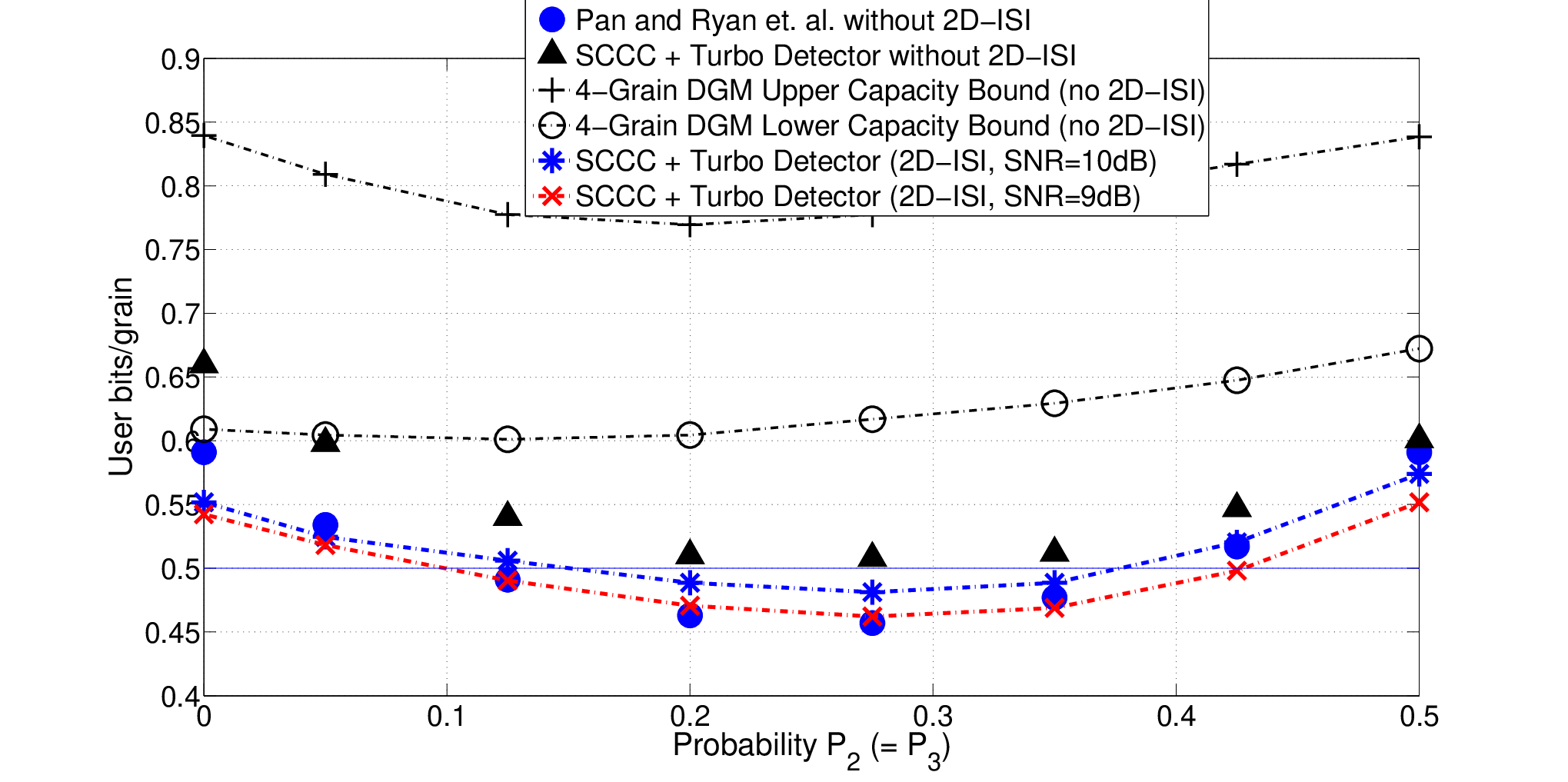
In Fig. 11, the horizontal axis represents the value of and the vertical axis represents the value of user bits per grain, which is twice the code rate. The triangle marker represents the performance of the system with no 2D-ISI (or additive noise) and is reproduced from [5]. The asterisk marker with dash-dotted line is the corresponding result for the system with 2D-ISI and additive noise with 10dB SNR. Results for 9 dB SNR are depicted with an ’X’ and dash-dotted line. Lower and upper bounds (from [2]) on the channel capacity of the 4-grain DGM TDMR channel (without 2D-ISI and AWGN) are shown with the open-circle and ’+’ markers, respectively.
|
| ||||||||||||||||||
|
|
|
|
|
| ||||||||||||||
| 0 | 16.4% | -6.6% | 15.59dB | 17.8% | -8.2% | 14.67dB | |||||||||||||
| 0.05 | 12.3% | -1.7% | 15.81dB | 13.4% | -2.9% | 14.86dB | |||||||||||||
| 0.125 | 6.3% | 3.0% | 15.97dB | 9.2% | -0.1% | 15.10dB | |||||||||||||
| 0.2 | 4.2% | 5.5% | 16.12dB | 7.7% | 1.6% | 15.28dB | |||||||||||||
| 0.275 | 5.3% | 5.3% | 16.19dB | 9.0% | 1.1% | 15.36dB | |||||||||||||
| 0.35 | 4.6% | 2.4% | 16.12dB | 8.4% | -1.7% | 15.30dB | |||||||||||||
| 0.425 | 4.9% | 0.6% | 15.85dB | 8.9% | -3.7% | 15.04dB | |||||||||||||
| 0.5 | 4.5% | -2.8% | 15.42dB | 8.2% | -6.6% | 14.59dB | |||||||||||||
Table I shows the code rate penalty (as a percentage) of the system with 2D-ISI and AWGN with respect to the TDMR/SCCC system without 2D-ISI and AWGN, along with the code rate gain (as a percentage) with respect to the system proposed by Pan and Ryan et. al. [3]. The SNR (4) used in Fig. 11 is per codeword bit. Table I also shows the SNR per information bit (taking into account the code rate) for both the 9 and 10 dB curves in Fig. 11. Compared to the result of pure TDMR case, the performance degradation due to 2D-ISI and additive noise is obvious and expected. At the left end, for values of 0 and 0.125, the decrease in code rate performance due to 2D-ISI and noise is relatively large—12% to 16% at 10 dB and 13% to 18% at 9 dB. For the central part of axis, where the model achieves a closer approximation of real magnetic grain channel, our system with 2D-ISI and additive noise outperforms the results published by Pan, Ryan et. al. —shown with filled circle marker—with no 2D-ISI or additive noise. At 10 dB SNR, the minimum density of 0.48 user bits per grain achieved by our combined iterative detector/equalizer/decoder occurs at a value of 0.275, and corresponds to an on-disk areal density of about 9.6 Terabits/, under the typically assumed media grain density of 20 Teragrains/. Thus, our simulation results support the feasibility of TDMR at densities of about 10 Terabits/, as proposed in [1].
VI Conclusion
This paper introduces a system for iterative detection, equalization, and decoding of two-dimensional magnetic recording channels in the presence of 2D-ISI and AWGN. It consists of a 2D-ISI equalizer, a TDMR detector based on a rectangular 4-grain DGM, and a SCCC decoder. The equalization algorithm uses joint extrinsic information to tackle the 2D-ISI and AWGN in a TDMR corrupted grain image. Methods for incorporating extrinsic information passed between the 2D-ISI and TDMR modules are presented. Optimal settings for some of the parameters of the system (e.g., weight factor applied on LLRs sent from 2D-ISI equalizer to TDMR detector, and the iteration schedule in the SCCC decoder) are obtained using an EXIT chart method. Performance of the optimized system is presented and compared to that of previously published results for equivalent TDMR channels without 2D-ISI. For the most part, the proposed system with 2D-ISI outperforms these previously published results. The presented simulations suggest that practical TDMR systems can achieve the density of 10 Terabits/ predicted in earlier publications; however, it must be noted that the rectangular DGM is somewhat simplistic compared to actual grain shapes. Future work will consider more realistic grain models and higher performance codes like LDPC codes. The capacity of the combined TDMR/2D-ISI channel described by (2) and (3) remains an open problem.
Acknowledgment
This work was supported by NSF grants CCF-1218885 and CCF-0635390. The authors also wish to acknowledge useful discussions with Dr. Roger Wood of Hitachi Global Storage Technologies, San Jose, CA.
References
- [1] R. Wood, M. Williams, A. Kavcic, and J. Miles, “The feasibility of magnetic recording at 10 terabits per square inch on conventional media,” IEEE Trans. Magnetics, vol. 45, no. 2, pp. 917–923, Feb. 2009.
- [2] A. Kavcic, X. Huang, B. Vasic, W. Ryan, and M. F. Erden, “Channel modeling and capacity bounds for two-dimensional magnetic recording,” IEEE Trans. Magnetics, vol. 46, no. 3, pp. 812–818, Mar. 2010.
- [3] L. Pan, W. E. Ryan, R. Wood, and B. Vasic, “Coding and detection for rectangular-grain TDMR models,” IEEE Trans. Magnetics, vol. 47, no. 6, pp. 1705–1711, June 2011.
- [4] L. R. Bahl, J. Cocke, F. Jelinek, and J. Raviv, “Optimal decoding of linear codes for minimizing symbol error rate,” IEEE Transactions on Information Theory, vol. 20, pp. 284–287, March 1974.
- [5] M. Carosino, Y. Chen, B. J. Belzer, K. Sivakumar, J. Murray, and P. Wettin, “Iterative detection and decoding for the four-rectangular-grain TDMR model,” in Proceedings of the Allerton Conference on Communication, Control, and Computing (accepted, to appear), 2013, also available at http://arxiv.org/abs/1309.7518.
- [6] Y. Chen, B. J. Belzer, and K. Sivakumar, “Iterative row-column soft-decision feedback algorithm using joint extrinsic information for two-dimensional intersymbol interference,” in Proceedings of the 44th Annual Conference on Information Sciences and Systems (CISS 2010), Princeton, NJ, March 2010, pp. 1–6.
- [7] ——, “Iterative soft-decision feedback zigzag algorithm using joint extrinsic information for two-dimensional intersymbol interference,” in Proceedings of the 45th Annual Conference on Information Sciences and Systems (CISS 2011), Baltimore, MD, March 2011, pp. 1–6.
- [8] S. ten Brink, “Convergence behavior of iteratively decoded parallel concatenated codes,” IEEE Trans. Commun., vol. 49, no. 10, pp. 1727–1737, Oct. 2001.