D. Aristoff, T. Lelièvre, and G. SimpsonParRep for simulating Markov chains
daristof@umn.edu
The parallel replica method for simulating long trajectories of Markov chains
Abstract
The parallel replica dynamics, originally developed by A.F. Voter, efficiently simulates very long trajectories of metastable Langevin dynamics. We present an analogous algorithm for discrete time Markov processes. Such Markov processes naturally arise, for example, from the time discretization of a continuous time stochastic dynamics. Appealing to properties of quasistationary distributions, we show that our algorithm reproduces exactly (in some limiting regime) the law of the original trajectory, coarsened over the metastable states.
keywords
Markov chain, parallel computing, parallel replica dynamics, quasistationary distributions, metastability1 Introduction
We consider the problem of efficiently simulating time homogeneous Markov chains with metastable states: subsets of state space in which the Markov chain remains for a long time before leaving. By a Markov chain we mean a discrete time stochastic process satisfying the Markov property. Heuristically, a set is metastable for a given Markov chain if the Markov chain reaches local equilibrium in much faster than it leaves . We will define local equilibrium precisely below, using quasistationary distributions (QSDs). The simulation of an exit event from a metastable state using a naive integration technique can be very time consuming.
Metastable Markov chains arise in many contexts. The dynamics of physical systems are often modeled by memoryless stochastic processes, including Markov chains, with widespread applications in physics, chemistry, and biology. In computational statistical physics (which is the main application field we have in mind), such models are used to understand macroscopic properties of matter, starting from an atomistic description. The models can be discrete or continuous in time. The discrete in time case has particular importance: even when the underlying model is continuous in time, what is simulated in practice is a Markov chain obtained by time discretization. In the context of computational statistical physics, a widely used continuous time model is the Langevin dynamics [17], while a popular class of discrete time models are the Markov State Models [24, 7]. For details, see [25, 17]. For examples of discrete time models not obtained from an underlying continuous time dynamics, see [26, 5]. In this article, we propose an efficient algorithm for simulating metastable Markov chains over very long time scales. Even though one of our motivations is to treat time discretized versions of continuous time models, we do not discuss errors in exit events due to time discretization; we refer for example to [4] and references therein for an analysis of this error.
In the physical applications above, metastability arises from the fact that the microscopic time scale (i.e., the physical time between two steps of the Markov chain) is much smaller than the macroscopic time scale of interest (i.e., the physical time to observe a transition between metastable states). Both energetic and entropic barriers can contribute to metastability. Energetic barriers correspond to high energy saddle points between metastable states in the potential energy landscape, while entropic barriers are associated with narrow pathways between metastable states; see Figure 1.
Many algorithms exist for simulating metastable stochastic processes over long time scales. One of the most versatile such algorithms is the parallel replica dynamics (ParRep) developed by A.F. Voter and co-workers [29, 30]. ParRep can be used with both energetic and entropic barriers, and it requires no assumptions about temperature, barrier heights, or reversibility. The algorithm was developed to efficiently compute transitions between metastable states of Langevin dynamics. For a mathematical analysis of ParRep in its original continuous time setting, see [27, 16]. In this article, we present an algorithm which is an adaptation of ParRep to the discrete time setting. It applies to any Markov chain.
ParRep uses many replicas of the process, simulated in parallel asynchronously, to rapidly find transition pathways out of metastable states. The gain in efficiency over direct simulation comes from distributing the computational effort across many processors, parallelizing the problem in time. The cost is that the trajectory becomes coarse-grained, evolving in the set of metastable states instead of the original state space. The continuous time version of ParRep has been successfully used in a number of problems in materials science (see e.g. [28, 22, 23, 18, 13, 15, 1]), allowing for atomistic resolution while also reaching extended time scales of microseconds, s. For reference, the microscopic time scale – typically the period of vibration of bond lengths – is about s.
In the continuous time case, consistency of the algorithm relies on the fact that first exit times from metastable states are exponentially distributed. Thus, if independent identically distributed (i.i.d.) replicas have first exit times , , then has the same law as . Now if is the first replica which leaves the metastable state amongst all the replicas, then the simulation clock is advanced by , and this time agrees in law with the original process. In contrast, in the discrete time case, the exit times from metastable states are geometrically distributed. Thus, if are now the geometrically distributed first exit times, then does not agree in law with . A different function of the must be found instead. This is our achievement with Algorithm 3.1 and Proposition 4.6. Our algorithm is based on the observation that agrees in law with .
2 Quasistationary Distributions
Throughout this work, will be a time homogeneous Markov chain with values in a probability space . For a random variable and probability measure , we write to indicate is distributed according to . For random variables and , we write when is a random variable with the same law as . We write and to denote probabilities and expectations for the Markov chain starting from the indicated initial distribution: . In the case that , we write and to denote probabilities and expectations for the Markov chain starting from .
To formulate and apply ParRep, we first need to define the metastable subsets of , which we will simply call states. The states will be used to coarse-grain the dynamics.
Definition 2.1.
Let be the collection of states, which we assume are disjoint bounded measurable subsets of . We write for a generic element of , and for the quotient map identifying the states.
As we will be concerned with when the chain exits states, we define the first exit time from ,
Much of the algorithm and analysis depends on the properties of the QSD, which we now define.
Definition 2.2.
A probability measure with support in is a QSD if for all measurable and all ,
| (1) |
Of course both and depend on , but for ease of notation, we do not make this explicit. The QSD can be seen as a local equilibrium reached by the Markov chain, conditioned on the event that it remains in the state. Indeed, it is easy to check that if is a measure with support in such that,
| (2) |
then is the QSD, which is then unique. In Section 4.1, we give sufficient conditions for existence and uniqueness of the QSD and for the convergence (2) to occur (see Theorem 4.2). We refer the reader to [6, 9, 20, 21, 16, 8] for additional properties of the QSD.
3 The Discrete Time ParRep Algorithm
Using the notation of the previous section, the aim of the ParRep algorithm is to efficiently generate a trajectory evolving in which has, approximately, the same law as the reference coarse-grained trajectory . Two of the parameters in the algorithm – and , called the decorrelation and dephasing times – depend on the current state , but for ease of notation we do not indicate this explicitly. See the remarks below Algorithm 3.1.
Algorithm 3.1.
Initialize a reference trajectory . Let be a fixed number of replicas and a fixed polling time at which the replicas resynchronize. Set the simulation clock to zero: . A coarse-grained trajectory evolving in is obtained by iterating the following:
HTML]E9F0E9
Decorrelation Step: Evolve the reference trajectory until it spends consecutive time steps in some state . Then proceed to the dephasing step. Throughout this step, the simulation clock is running and the coarse-grained trajectory is given by
| (3) |
HTML]E9F0E9
Dephasing Step: The simulation clock is now stopped and the reference and coarse-grained trajectories do not evolve. Evolve independent replicas starting at some initial distribution with support in , such that whenever a replica leaves it is restarted at the initial distribution. When a replica spends consecutive time steps in , stop it and store its end position. When all the replicas have stopped, reset each replica’s clock to and proceed to the parallel step.
HTML]E9F0E9
Parallel Step: Set and iterate the following:
- 1.
Evolve all replicas from time to time . The simulation clock is not advanced in this step.
- 2.
If none of the replicas leaves during this time, update and return to 1, above.
Otherwise, let be the smallest number such that leaves during this time, let be the corresponding (first) exit time, and set
(4) Update the coarse-grained trajectory by
(5) and the simulation clock by . Set , and return to the decorrelation step.
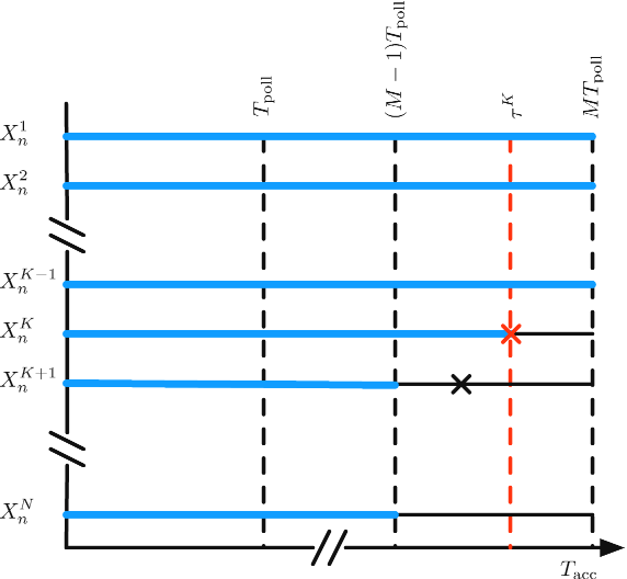
The idea of the parallel step is to compute the exit time from as the sum of the times spent by the replicas up to the first exit observed among the replicas. More precisely, if we imagine the replicas being ordered by their indices ( through ), this sum is over all replicas up to the last polling time, and then over the first replicas in the last interval between polling times, being the smallest index of the replicas which are the first to exit. Notice that and are such that . See Figure 2 for a schematic of the Parallel Step. We comment that the formula for updating the simulation time in the parallel step of the original ParRep algorithm is simply .
A few remarks are in order (see [27, 16] for additional comments on the continuous time algorithm):
- The Decorrelation Step.
-
In this step, the reference trajectory is allowed to evolve until it spends a sufficiently long time in a single state. At the termination of the decorrelation step, the distribution of the reference trajectory should be, according to (2), close to that of the QSD (see Theorem 4.2 in Section 4.1).
The evolution of the reference trajectory is exact in the decorrelation step, and so the coarse-grained trajectory is also exact in the decorrelation step.
- The Dephasing Step.
-
The purpose of the dephasing step is to generate i.i.d. samples from the QSD. While we have described a simple rejection sampling algorithm, there is another technique [3] based on a branching and interacting particle process sometimes called the Fleming-Viot particle process [11]. See [2, 19, 9, 12, 21] for studies of this process, and [3] for a discussion of how the Fleming-Viot particle process may be used in ParRep.
In our rejection sampling we have flexibility on where to initialize the replicas. One could use the position of the reference chain at the end of the decorrelation step, or any other point in .
- The Decorrelation and Dephasing Times.
-
and must be sufficiently large so that the distributions of both the reference process and the replicas are as close as possible to the QSD, without exhausting computational resources. and play similar roles, and they both depend on the initial distribution of the processes in .
Choosing good values of these parameters is nontrivial, as they determine the accuracy of the algorithm. In [3], the Fleming-Viot particle process together with convergence diagnostics are used to determine these parameters on the fly in each state. They can also be postulated from some a priori knowledge (e.g., barrier height between states), if available.
- The Polling Time.
-
The purpose of the polling time is to permit for periods of asynchronous computation of the replicas in a distributed computing environment. For the accelerated time to be correct, it is essential that all replicas have run for at least as long as replica . Ensuring this requires resynchronization, which occurs at the polling time.
If communication amongst the replicas is cheap or there is little loss of synchronization per time step, one can take . In this case, is the first exit time observed among the replicas, (so ) and .
- Efficiency of the Algorithm.
-
For the algorithm to be efficient, the states must be truly metastable: within each state, the typical time to reach the QSD ( and ) should be small relative to the typical exit time. If most states are not metastable, then the exit times will be typically smaller than the decorrelation times, and the algorithm will rarely proceed to the dephasing and parallel steps.
The algorithm is consistent even if some or all the states are not metastable. Indeed, the states can be any collection of disjoint sets. However, if these sets are not reasonably defined, it will be difficult to obtain any gain in efficiency with ParRep. Defining the states requires some a priori knowledge about the system.
4 Mathematical Analysis of Discrete Time ParRep
The main result of this section, Proposition 4.6, shows that the coarse-grained trajectory simulated in ParRep is exact if the QSD has been exactly reached in the decorrelation and dephasing steps; see Equation (7) below.
4.1 Properties of Quasistationary Distributions
Before examining ParRep, we give a condition for existence and uniqueness of the QSD. We also state important properties of the exit law starting from the QSD. Many of these results can be found in [9, 8]. We assume the following, which is sufficient to ensure existence and uniqueness of the QSD.
Assumption 4.1.
Let be any state.
- 1.
For any ,
- 2.
There exists and , such that for all and all bounded non-negative measurable functions ,
With this condition, the following holds (see [10, Theorem 1]):
Theorem 4.2.
Under Assumption 4.1, there exists a unique QSD in . Furthermore, for any probability measure with support in and any bounded measurable function ,
| (6) |
Theorem 4.2 shows that the law of , conditioned on not exiting , converges in total variation norm to the QSD as . Thus, at the end of the decorrelation and dephasing steps, if and are sufficiently large, then the law of the reference process and replicas will be close to that of the QSD. Notice that Theorem 4.2 provides an explicit error bound in total variation norm.
Next we state properties of the exit law starting from the QSD which are essential to our analysis. While these results are well-known (see, for instance, [9, 8]), we give brief proofs for completeness.
Theorem 4.3.
If , with the QSD in , then and are independent, and is geometrically distributed with parameter .
4.2 Analysis of the exit event
We can now state and prove our main result. We make the following idealizing assumption, which allows us to focus on the the parallel step in Algorithm 3.1, neglecting the errors due to imperfect sampling of the QSD.
Idealization 4.5.
Assume that:
- (A1)
After spending consecutive time steps in , the process is exactly distributed according to the QSD in . In particular, at the end of the decorrelation step, .
- (A2)
At the end of the dephasing step, all replicas are i.i.d. with law exactly given by .
Idealization 4.5 is introduced in view of Theorem 4.2, which ensures that the QSD sampling error from the dephasing and decorrelation steps vanishes as and become large. Of course, for finite and , there is a nonzero error; this error will indeed propagate in time, but it can be controlled in terms of these two parameters. For a detailed analysis in the continuous time case, see [27, 16]. Though the arguments in [27, 16] could be adapted to our time discrete setting, we do not go in this direction; instead we focus on showing consistency of the parallel step.
Under Idealization 4.5, we show that ParRep is exact. That is, the trajectory generated by ParRep has the same probability law as the true coarse-grained chain:
| (7) |
The evolution of the ParRep coarse-grained trajectory is exact in the decorrelation step. Together with Idealization 4.5, this means (7) holds if the parallel step is consistent (i.e. exact, if all replicas start at i.i.d. samples of the QSD). This is the content of the following proposition.
Proposition 4.6.
To prove Proposition 4.6, we need the following lemma:
Lemma 4.7.
Let be i.i.d. geometric random variables with parameter : for ,
Define
Then has the same law as .
Proof 4.8.
Notice that can be rewritten as
Indeed, any natural number can be uniquely expressed as where , and . For such , and we compute
We can now proceed to the proof of Proposition 4.6.
Proof 4.9.
In light of Theorem 4.3, it suffices to prove:
- (i)
is a geometric random variable with parameter ,
- (ii)
and have the same law: , and
- (iii)
is independent of ,
where is the process starting at the .
We first prove (i). For , let be a random variable representing the first exit time from of the th replica in the parallel step of ParRep, if the replica were allowed to keep evolving indefinitely. By (A2), are independent and all have the same distribution as . Now by Theorem 4.3, are i.i.d. geometric random variables with parameter , so by Lemma 4.7, is also a geometric random variable with parameter .
Now we turn to (ii) and (iii). Note that if and only if and there exists such that , , and . From Theorem 4.3 and (A2), is independent of , so must be independent of . From this and (A2), it follows that . To see that is independent of , let be the sigma algebra generated by and . Knowing the value of and is enough to deduce the value of ; that is, is -measurable. Also, by the preceding analysis and Theorem 4.3, is independent of . To conclude that and are independent, we compute for suitable test functions and :
5 Numerical Examples
In this section we consider two examples. The first illustrates numerically the fact that the parallel step in Algorithm 3.1 is consistent. The second shows typical errors resulting from a naive application of the original ParRep algorithm to a time discretization of Langevin dynamics. These are simple illustrative numerical examples. For a more advanced application, we refer to the paper [3], where our Algorithm 3.1 was used to study the 2D Lennard-Jones cluster of seven atoms.
5.1 One-dimensional Random Walk
Consider a random walk on with transition probabilities defined as follows:
We use ParRep to simulate the first exit time of the random walk from , starting from the QSD in . At each point except , steps towards are more likely than steps towards the boundaries or .
We perform this simulation by using the dephasing and parallel steps of Algorithm 3.1; for sufficiently large , the accelerated time should have the same law as . In this simple example we can analytically compute the distribution of . We perform independent ParRep simulations to obtain statistics on the distribution of and the gain in “wall clock time,” defined below. We find that and have very close probability mass functions when ; see Figure 3. To measure the gain in wall clock efficiency using ParRep, we introduce the parallel time – defined, using the notation of Algorithm 3.1, by , where we recall is such that . Thus, the wall clock time of the parallel step is , with the computational cost of a single time step of the Markov chain for one replica. Note in Figure 4 the significant parallel time speedup in ParRep compared with the direct sampling time. The speedup is approximately linear in .
5.2 Discretized Diffusions
Consider the overdamped Langevin stochastic process in ,
| (8) |
The associated Euler-Maruyama discretization is
| (9) |
where are -dimensional i.i.d. random variables. It is well-known [14] that is then an approximation of .
5.2.1 Existence and uniqueness of the QSD
Proof 5.2.
First, for any ,
| (10) |
Next, for any ,
| (11) |
where
Since is bounded and terms in the brackets are bounded, . In Assumption 4.1 we can then take and .
Theorem 4.2 ensures that converges to a unique QSD in , with a precise error estimate in terms of the parameters and obtained in the proof of Proposition 5.1 . This error estimate is certainly not sharp; better estimates can be obtained by studying the spectral properties of the Markov kernel. We refer to [16] for such convergence results in the continuous time case (8).
5.2.2 Numerical example
Here we consider the 1D process
| (12) |
discretized with . We compute the first exit time from , starting at . We use Algorithm 3.1 with , corresponding to the physical time scale , and replicas.
Consider a direct implementation of the continuous time ParRep algorithm into the time discretized process. In that algorithm, the accelerated time is (in units of physical time instead of time steps)
| (13) |
with the same as in Algorithm 3.1 above. As is by construction a multiple of , a staircasing effect can be seen in the exit time distribution; see Figure 5. This staggering worsens as the number of replicas increases. In our Algorithm 3.1, we use the accelerated time formula (again in units of physical time)
We find excellent agreement between the serial data – that is, the data obtained from direct numerical simulation – and the data obtained from Algorithm 3.1. See Figure 5. (The agreement is perfect in the decorrelation step; see Figure 6.) We comment further on this in the next section.
5.2.3 Discussion
In light of the discretization example, one may ask what kind of errors were introduced in previous numerical studies which used ParRep with (13). Taking for simplicity, we calculate
Using calculations analogous to those used to study , it can be shown that
Therefore the error in the number of time steps per parallel step is
| (14) |
Consider the relative error, writing it as
We claim the quantity in the brackets,
| (15) |
is bounded from above by one. Indeed, for any , we immediately see that is zero at and one as . Let us reason by contradiction and assume that . Since is continuous in and , there is then a point such that ; thus
Note that and for all values of . Computing the derivative with respect to , we observe
Therefore, is decreasing, from one at to zero at , in the interval . Hence, has no solution, contradiction. We conclude that (15) is bounded from above by one.
Consequently, we are assured
| (16) |
Thus, so long as , the relative error using the accelerated time will be modest, especially for very metastable states where . If also , then the absolute error will be small.
The above calculations are generic. Though our discretized diffusion example in Section 5.2.2 is a simple 1D problem, the errors displayed in Figure 5 are expected whenever the continuous time ParRep rule (13) is used for a time discretized process. Though this error (as we showed above) will be small provided and , our Algorithm 3.1 has the advantage of being consistent for any , including relatively large values of .
Acknowledgments
We would like to thank the anonymous referees for their many constructive remarks. The work of D. Aristoff and G. Simpson was supported in part by DOE Award DE-SC0002085. G. Simpson was also supported by the NST PIRE Grant OISE-0967140. The work of T. Lelièvre is supported by the European Research Council under the European Union’s Seventh Framework Programme (FP/2007-2013) / ERC Grant Agreement number 614492.
References
- [1] K.L. Baker and D.H. Warner. Extended timescale atomistic modeling of crack tip behavior in aluminum. Modelling And Simulation In Materials Science And Engineering, 20(6):065005, 2012.
- [2] M. Bieniek, K. Burdzy, and S. Finch. Non-extinction of a Fleming-Viot particle model. Probability Theory and Related Fields, 153(1-2):293–332, 2012.
- [3] A.J. Binder, T. Lelièvre, and G. Simpson. A generalized Parallel Replica dynamics. Preprint arXiv:1404.6191, 2014.
- [4] B. Bouchard, S. Geiss, and E. Gobet. First time to exit of a continuous Itô process: general moment estimates and -convergence rate for discrete time approximations, 2013. Preprint http://hal.archives-ouvertes.fr/hal-00844887.
- [5] A. Bovier, M. Eckhoff, V. Gayrard, and M. Klein. Metastability and low lying spectra in reversible Markov chains. Communications in Mathematical Physics, 228(2):219–255, 2002.
- [6] P. Cattiaux, P. Collet, A. Lambert, S. Martínez, S. Méléard, and J. San Martín. Quasi-stationary distributions and diffusion models in population dynamics. The Annals of Probability, 37(5):1926–1969, 2009.
- [7] J.D. Chodera, N. Singhal, V.S. Pande, K.A. Dill, and W.C. Swope. Automatic discovery of metastable states for the construction of Markov models of macromolecular conformational dynamics. The Journal of Chemical Physics, 126(15):155101, 2007.
- [8] P. Collet, S. Martinez, and J. San Martin. Quasi-Stationary Distributions. Springer, 2013.
- [9] P. Del Moral. Feynman-Kac Formulae. Springer, 2004.
- [10] P. Del Moral and A. Doucet. Particle motions in absorbing medium with hard and soft obstacles. Stochastic Analysis and Applications, 22(5):1175–1207, 2004.
- [11] P.A. Ferrari and N. Maric. Quasi stationary distributions and Fleming-Viot processes in countable spaces. Electron. J. Probab., 12(24):684–702, 2007.
- [12] I. Grigorescu and M. Kang. Hydrodynamic limit for a Fleming-Viot type system. Stochastic Processes and Their Applications, 110(1):111–143, 2004.
- [13] K.L. Joshi, S. Raman, and A.C.T. van Duin. Connectivity-based parallel replica dynamics for chemically reactive systems: From femtoseconds to microseconds. The Journal of Physical Chemistry Letters, 4(21):3792–3797, 2013.
- [14] P.E. Kloeden and E. Platen. Numerical Solution of Stochastic Differential Equations. Springer, 1992.
- [15] R. Komanduri, N. Chandrasekaran, and L. Raff. Molecular dynamics simulation of atomic-scale friction. Physical Review B, 61(20):14007–14019, 2000.
- [16] C. Le Bris, T. Lelièvre, M. Luskin, and D. Perez. A mathematical formalization of the parallel replica dynamics. Monte Carlo Methods and Applications, 18(2):119–146, 2012.
- [17] T. Lelièvre, G. Stoltz, and M. Rousset. Free Energy Computations: A Mathematical Perspective. Imperial College Press, 2010.
- [18] C.-Y. Lu, A.F. Voter, and D. Perez. Extending atomistic simulation timescale in solid/liquid systems: Crystal growth from solution by a parallel-replica dynamics and continuum hybrid method. The Journal of Chemical Physics, 140(4):044116, 2014.
- [19] B. Mariusz, Krzysztof B., and P. Soumik. Extinction of Fleming-Viot-type particle systems with strong drift. Electron. J. Probab., 17:no. 11, 1–15, 2012.
- [20] S. Martínez and J. San Martín. Quasi-stationary distributions for a Brownian motion with drift and associated limit laws. Journal of Applied Probability, 31(4):911–920, 1994.
- [21] S. Méléard and D. Villemonais. Quasi-stationary distributions and population processes. Probability Surveys, 9:340–410, 2012.
- [22] D. Perez, Y. Dong, A. Martini, and A.F. Voter. Rate theory description of atomic stick-slip friction. Physical Review B, 81(24):245415, 2010.
- [23] D. Perez, S.-N. Luo, A.F. Voter, and T.C. Germann. Entropic Stabilization of Nanoscale Voids in Materials under Tension. Physical Review Letters, 110(20):206001, 2013.
- [24] J.-H. Prinz, H. Wu, M. Sarich, B. Keller, M. Senne, M. Held, J.D. Chodera, C. Schütte, and F. Noé. Markov models of molecular kinetics: Generation and validation. The Journal of Chemical Physics, 134(17):174105, 2011.
- [25] C. Schütte and M. Sarich. Metastability and Markov State Models in Molecular Dynamics. AMS, 2013.
- [26] E. Scoppola. Metastability for Markov chains: A general procedure based on renormalization group ideas. In G. Grimmett, editor, Probability and Phase Transition, volume 420 of NATO ASI Series, pages 303–322. Springer Netherlands, 1994.
- [27] G. Simpson and M. Luskin. Numerical Analysis of Parallel Replica Dynamics. M2AN, 47:1287–1314, 2013.
- [28] B.P. Uberuaga, S.J. Stuart, and A.F. Voter. Parallel replica dynamics for driven systems: Derivation and application to strained nanotubes. Physical Review B, 75(1):014301, 2007.
- [29] A.F. Voter. Parallel replica method for dynamics of infrequent events. Phys. Rev. B, 57(22):13985–13988, 1998.
- [30] A.F. Voter, F. Montalenti, and T.C. Germann. Extending the time scale in atomistic simulation of materials. Annual Review of Materials Science, 32:321–346, 2002.