Dynamical Models of Elliptical Galaxies – II. M87 and its Globular Clusters
Abstract
We study the Globular Cluster (GC) system of the nearby elliptical galaxy M87 using the newly available dataset with accurate kinematics provided by Strader et al. (2011). We find evidence for three distinct sub-populations of GCs in terms of colours, kinematics and radial profiles. We show that a decomposition into three populations – blue, intermediate and red GCs – is statistically preferred to one with two or four populations. The existence of three components has been suggested before, but here we are able to identify them robustly and relate them to the stellar profile. We exploit the sub-populations to derive dynamical constraints on the mass and Dark Matter (DM) content of M87 out to kpc. We deploy a class of global mass-estimators, developed in Paper I, obtaining mass measurements at different locations. The DM fraction in M87 changes from 0.2 at the effective radius of the stellar light ( or 6 kpc) to 0.95 at the distance probed by the most extended, blue GCs ( or 135 kpc).
We supplement this analysis with virial decompositions, which exploit the dynamical model to produce a separation into multiple components. These yield the luminous mass as and the dark matter within 135 kpc as The inner DM density behaves as with . This is steeper than the cosmologically preferred cusp of (Dubinski & Carlberg; Navarro, Frenk & White), and may provide evidence of dark matter contraction. Finally, we combine the GC separation into three sub-populations with the Jeans equations, obtaining information on the orbital structure of the GC system. The centrally concentrated red GCs exhibit tangential anisotropy, consistent with the depletion of radial orbits by tidal shredding. The most extended blue GCs have an isotropic velocity dispersion tensor in the central parts, which becomes more tangential moving outwards, consistent with adiabatic contraction of the DM halo.
1 Introduction
Elliptical galaxies and their dark matter (DM) haloes provide crucial tests of galaxy formation scenarios. The different phases of assembly (Johansson et al ., 2012; Hilz et al., 2013), the interplay between luminous and dark components over different timescales (Blumenthal et al., 1986; Abadi et al., 2010; Zubovas & King, 2012), as well as the initial conditions (Stiavelli & Bertin, 1987; Nipoti et al., 2012; Remus et al., 2013) all leave imprints on the final profiles. However, some properties of present-day ellipticals are not straightforward to obtain. For example, the orbital distribution of stars and the DM halo profile are not directly accessible. These must be derived by modelling the observed photometry and line-of-sight (LOS) kinematics, and are generally degenerate with one another (mass-anisotropy degeneracy).
Additional information on the mass profile can be gathered through the kinematics of Globular Clusters (GCs) and Planetary Nebulae (PNe). This has been possible thanks to dedicated observational campaigns and instrumentation (Douglas et al., 2002, such as the PN.Spectrograph,). Observations of PNe probe the photometric and kinematic profiles of the starlight well beyond the effective radius, where the surface-brightness would be too low (Coccato et al., 2009). Globular Cluster populations typically extend out to larger radii and, if their distribution and/or kinematics differ from those of the starlight, can be exploited as independent tracers of the same gravitational potential.
Use of GC or PN kinematics as a mass constraint dates back to Mould et al. (1987) and has been applied to a diverse set of early-type galaxies since then (Pota et al., 2013, e.g.), to infer masses and properties of the DM haloes (Napolitano et al., 2009; Schuberth et al., 2010; Deason et al., 2012) or validate galaxy formation scenarios (Coccato et al., 2009; Schuberth et al., 2012). The models have relied on the Jeans equations or on distribution functions to reproduce the velocity dispersions and, in some cases, higher-order moments of the LOS velocity distribution. Perhaps the most complete method is given by orbit-based (Schwarzschild, 1979, hereafter S79) and made-to-measure modelling (Syer & Tremaine, 1996; Morganti et al., 2013). We will call these forward techniques, to emphasize that they consist in building three-dimensional densities and velocities, which are then compared to the projected observables (surface density, velocity dispersion and higher-order moments).
However, conclusions on the dynamical side are weakened by the mass-anisotropy degeneracy, such as in the controversy over DM fractions and orbital structure (Romanowsky et al., 2003; Dekel et al., 2005). Also, the sample size and accuracy of kinematic measurements play a key role. For reference, reliable inference on the LOS velocity distribution and its higher moments requires a lower limit of tracers per radial bin (Amorisco & Evans, 2012), a condition which is not always met in practice. Especially with the limited number of GCs per host galaxy, only marginal conclusions on the orbital structure can be drawn from analyses of the higher-order moments. In the analogous context of resolved stellar populations in dwarf spheroidals (dSphs), where larger datasets are available, significant improvements have been brought by the identification of multiple populations and the use of global estimators, sometimes with sharper performance than more refined analyses in which all sub-populations were grouped together as a whole (Walker & Peñarrubia, 2011; Agnello & Evans, 2012b; Amorisco et al., 2013). The virial results can then be used as a prior on the dynamical parameters, to inform more detailed analyses whose outcome is mainly the orbital structure (Richardson & Fairbairn, 2013).
Moreover, forward techniques require a number of steps to relate the projected distribution on the sky to the projected kinematics. Given the generally low number of GCs or PNe per galaxy (a few hundred in the best cases, so far), the surface density distribution and kinematics of tracers can be very uncertain, adding to the computational complexity of some forward modelling techniques. In a companion paper (see Agnello et al., 2013b, hereafter Paper I), a novel approach has been illustrated. This is based upon a reformulation of the Jeans equations, which yields the predicted velocity dispersions and their aperture-averages by means of single or double integrals involving directly, along with a kernel that depends on the mass and anisotropy profiles. As a by-product, different mass estimators at particular locations have been derived, as well as characterisations of the kinematic profiles and common aperture-corrections (Jorgensen et al., 1995; Cappellari et al., 2006, cf). Some particular cases (the virial limit and isotropic tracers in power-law potentials) have been previously exploited in a variety of problems, ranging from gravitational lensing by galaxies (Agnello et al., 2013) to the DM profiles of dwarf spheroidals (Amorisco et al., 2013).
Here, we will apply the results of Paper I to the early-type galaxy M87 and its GC system. This is one of the most luminous and massive galaxies within 20 Mpc, and hosts one of the most populous GC systems. It was the first target of GC spectroscopy beyond the Local Group (Mould et al., 1987; Mould et al., 1990; Huchra & Brodie, 1987). Since then, its GCs have been studied extensively, most notably with larger kinematic samples by Cohen & Ryzhov (1997), Cohen (2000) and Hanes et al. (2001). Interest then turned to other galaxies until Strader et al. (2011, hereafter S11) revisited M87 with a new generation of of high resolution, high signal-to-noise spectroscopy, providing the largest, publicly available, sample in the literature. This is the dataset we will use here.
In Section 2, we introduce the dataset that will be used in the subsequent dynamical analyses and summarize previous results in the literature. In Section 3, we present a partition into sub-populations, showing that the GC system of M87 is most likely a superposition of three distinct (and internally homogeneous) sub-populations. In Section 4, we use the three GC populations to obtain virial constraints on the mass profile (luminous mass, DM fractions, DM contraction) in a manner that is independent of any orbital structure. In Section 5, we then apply the integral form of the Jeans equations derived in Paper I to learn about the orbital distributions. We comment and draw conclusions in Section 6.
From now on, we adopt a systemic velocity of 1307 kms-1 and a distance of 16.5 Mpc for M87 (Madrid et al., 2009; Bird et al., 2010, see e.g.,). Throughout all this paper, fits and likelihood explorations are performed using the Markov Chain Monte Carlo technique.
2 M87 and its Globular Clusters
The S11 data were based on wide-field imaging from11 1 Acronyms: CHFT, Canada-France-Hawaii Telescope; DEIMOS, DEep Imaging Multi-Object Spectrograph; MMT, Multiple Mirror Telescope. See S11 and references therein. Subaru/Suprime-Cam and CFHT/MegaCam, with follow-up spectroscopy on Keck/DEIMOS and MMT/Hectospec out to 185 kpc ( degrees). These data have undergone extensive vetting for reliability and the velocities are accurate at the kms-1 level. Comparison to the older generation of data (performed by S11) was however revealing. Several cases of ‘catastrophic’ errors were found, with differences up to km/s that seem most likely to be problems with the older data on a smaller telescope. Unfortunately, even a few such unrecognized errors can have dramatic impacts on kinematic parameters such as the velocity dispersion, with subsequent repercussions on the dynamical mass. In particular, the GC dispersion profile of M87 was previously thought to rise rapidly with radius, but with the newer data it is seen to remain constant or decline (as shown below and in S11).
The kinematics of smaller datasets of GCs at smaller radii have already been studied before. Cohen & Ryzhov (1997) performed a Jeans analysis, assuming an isotropic velocity dispersion tensor, on 205 GCs between and degrees (i.e. ). They used a power-law model for the total density (i.e. luminous plus DM),
| (1) |
and inferred corresponding to a (total) mass profile . Romanowsky & Kochanek (2001) studied a set of GCs by means of S79 orbit modelling, finding evidence for a dark halo with density falling off more slowly than Wu & Tremaine (2006) applied a S79 orbit-based analysis, with a power-law total density, to a sample of GCs between and degrees. They found although the likelihood has three peaks, one of which is almost at The energy distribution resulting from their modelling suggested multiple distinct components, although the data were not enough to confirm this hypothesis robustly. Murphy et al. (2011) analysed 278 GCs up to kpc ( deg) by means of orbit-based methods, together with stellar kinematics for the starlight, as to infer the (total) mass profile over a wide radial range. The expected (total) mass at22 2 Or at 35 kpc with their adopted distance, which is 17.9 Mpc, whereas Wu & Tremaine (2006) assumed 16 Mpc. 32 kpc is higher than the one reported in Wu & Tremaine (2006). Also, mass-estimates from X-rays are almost lower than the ones inferred from GCs at small radii (Murphy et al., 2011).
Here, we make use of the S11 dataset, while omitting the brightest objects (with magnitude ) that may be a distinct population of ultra-compact dwarfs (as discussed in S11 and Brodie et al. 2011). We also do not make use of the additional DEIMOS data from Romanowsky et al. (2012), since these were specifically obtained around a cold substructure that could bias the kinematics. In particular, the sample with accurate kinematic measurements (the ‘kinematic’ sample) is a subset of the dataset studied in S11 (the ‘photometric’ sample).


Top: Surface density profiles of GCs in M87, after subtraction of contaminants. The full lines are given by the number-counts of Harris (2009), where the surface-density of contaminants is estimated directly from field objects; the dashed lines show the best-fitting profiles of S11, where an independent photometric sample was used, the fraction of contaminants was a free parameter in the modelling and the radial selection function was accounted for. Blue (dark red) denotes the GCs with lower (higher) than 0.93. Note that the redder GCs are more centrally concentrated.
Bottom: Line of sight velocities (relative to M87) versus distance from M87 for GCs in the spectroscopic subsample of S11. Redder (bluer) points mark GCs with higher (lower) values of
2.1 The Data
In order to exclude possible contaminants from our catalogue, we adopt the same criterion of Harris (2009) and S11, considering just those objects in the kinematic sample with colours as follows:
| (2) |
Our kinematic sub-sample consists of bona fide GCs, with positions, LOS velocities and colours. A clear bimodality is present in the colour distribution (as already observed in Harris, 2009, S11).
A priori, the selection function for the kinematic sub-sample may not be the same as for the photometric catalogue, both in positions and in colours. If this happened, the surface-density profiles used in the dynamical analysis would be inadequate and any mass measurements would be affected by that. Also, we must be confident that just the bona fide GCs are considered for the dynamical analysis. Harris (2009) and S11 examined different procedures to isolate the GCs, subtract the contaminants and separate the sample in bluer () and redder () sub-populations.
Figure 1 shows the estimated radial profiles, for bluer and redder GCs. The profiles given in S11 are consistent with the number counts for pure GCs estimated by Harris (2009) with a different procedure for contaminant subtraction. The surface-density profile of ‘red’ GCs matches smoothly to the starlight’s surface-brightness profile in the inner regions, suggesting that the starlight is associated with a red GC population. This fades at larger radii into a bluer, metal-poorer and less concentrated component, which may be the result of accretion onto M87 (Brodie & Strader, 2006).


In the dynamical analysis, we will use data from the kinematic sub-sample. Then, we need to know if the photometric profiles are consistent between the photometric sample and the kinematic subsample. Although the radial selection function is different, a simple check consists in examining the ratios of redder-to-bluer GCs at different locations, which depends just on the colour selection function. Figure 2 shows the ratio of redder-to-bluer GCs estimated by ratio of number-counts in different radial bins, both for the photometric and kinematic sub-samples. As the plots show, the kinematic sub-sample is a faithful representation of the total (photometric) sample without substantial colour biases or contamination in the distance range probed here.
3 Sub-populations
A simple colour separation based on hard cuts 33 3 That is, larger or smaller than the conventional value 0.93. shows that the bluer GCs have a higher velocity dispersion than the redder ones. Having both colours and LOS velocities, we can exploit them jointly to separate our sample into sub-populations.
We will suppose that each population has a Gaussian distribution in colour and velocity, of the kind
| (3) |
(c.f., Walker & Penarrubia 2011). We use the difference between and magnitudes as the colour in our study, while denotes the population, the line-of-sight velocity, the velocity dispersion and the mean colour and colour dispersion. The above distribution can be modified to distinguish between rotation and random motions. However, in what follows, we are primarily interested in the entirety of the second velocity moment, whether due to ordered or random motions, and this is the same as the dispersion estimated via eq. (3).
| bin | ||||||||
|---|---|---|---|---|---|---|---|---|
| (deg) | (kms-1 ) | (kms-1) | ||||||
| 85 | ||||||||
| 123 | ||||||||
| 78 | ||||||||
| 68 |


Top: Colour () parameters resulting from a bimodal fit in different bins of distance (horizontal error-bars), as in Sect.3.1 and Table 1. Full error-bars: mean colour and its uncertainty; dashed errorbars: width of the colour distribution, centered on the mean colour for visual convenience. The mean-colour variation of the ‘red’ GCs over distance is monotonic, appreciably larger than the uncertainties and is comparable to the colour dispersion, at variance with the behaviour of ‘blue’ GCs.
Bottom: Velocity dispersion profiles for GCs of different colours. Blue (yellow, red): GCs with ( Full lines mark the velocity dispersions computed via eq.(5), whilst dashed lines delimit the uncertainties computed by linear propagation on in eq.(5). The bin-size varies with radius, such that a quarter of the GC subpopulation is enclosed in each bin. GCs with show a sharp transition in which corresponds to the transition in mean colour of the redder GCs (top panel).
3.1 Bimodal Partition
We start by dividing our sample into four radial bins and performing a bimodal fit in each of them. We suppose that are reasonably uniform for each sub-population in each radial bin. In the bimodal fitting, each GC with measured velocity and colour gives a contribution
| (4) |
to the likelihood of the bimodal partition, with (or ) the fraction of ‘bluer’ (or ‘redder’) GCs in the radial bin considered. The final likelihood for the parameters is the product of individual contributions over all objects in the bin. Different possible bin sizes were investigated, with the aim of minimising uncertainties and bin size while keeping the number of GCs equal among different bins.
Table 1 summarises the outcome of our bimodal fitting and the bin sizes chosen. The blue fraction increases with radius, as expected based on Harris (2009) and S11. The ‘bluer’ sub-population has overall constant colour parameters and a smoothly declining velocity dispersion profile. The ‘redder’ GCs have a mean colour that decreases towards Also, their LOS kinematics shows an abrupt drop-off from kms-1 in the innermost bin to kms-1 at larger radii. This is accompanied by a significant change in the mean colour of the ‘redder’ sub-population. The inner value of the velocity dispersion is consistent with the kinematics of the stellar component (S11). Suppose the velocity dispersion of ‘redder’ GCs is estimated at different radii via a uniform smoothing kernel
| (5) |
where is the Heaviside function. Then, the dispersion still shows a sharp decrease for the ‘redder’ GCs, which does not have a counterpart in the ‘bluer’ ones (fig.3). On the other hand, the LOS kinematic profile for the starlight is approximately flat even beyond the effective radius, so we would not expect a sharp drop in for the red GCs either.
The following hypothesis emerges: the red GCs consist of a more compact (and redder) sub-population and a more extended, intermediate-colour sub-population. This hypothesis was suggested and supported also in Sections 5 and 6 of S11. Our sample is a subset44 4 Besides those used here, S11 included other GCs, with measurements already known from the literature but with unverified velocities. of the one considered by S11, which had been thoroughly examined to exclude contaminants or evident substructure and select just the GCs that are bound to M87. Here, we will make one further step and exploit this hypothesis to identify three dynamical tracer populations, which can be used to infer masses at different locations.
| parameter | blue | intermediate | red |
|---|---|---|---|
| (km/s) | |||
| (km/s) | |||
3.2 Three Populations
We proceed to a decomposition into three sub-populations, each of which has uniform colour parameters and velocity dispersion. We model each sub-population with a Sérsic profile for the surface number-density
| (6) |
and denote the fraction of th population at radius as
| (7) |
where we have added a new subscript ‘i’ to denote the intermediate population. The Sérsic coefficient is chosen such that is the effective radius of the th population, enclosing half the total (projected) number of GCs. In particular, we rely on the approximate expression listed in Ciotti & Bertin (1999) in terms of the Sérsic index
Then, a GC at radius will give a contribution to the likelihood
| (8) |
Just as for the bimodal fits, the likelihood of the parameters is the product of over all GCs in our sample. The likelihood is now a function of: effective radii and Sérsic indices of the populations; mean colours and colour dispersions; global velocity dispersions; and the ratios between the surface number densities at the centre. By studying the likelihood over the parameter space, we obtain both the best-fitting parameters and their distribution, including uncertainties.
Table 2 shows the colour parameters, mean velocity dispersions and photometric parameters. Uncertainties on the photometric parameters are large, especially for the effective radii. This was also observed in S11, where photometric profiles were sought for the bluer () and redder () GCs in the larger, photometric sample. Despite the uncertainties, some well-defined relations are satisfied among the parameters. In particular, the effective radius of the intermediate population is almost always smaller than that of the blue GCs (with ). Also, the velocity dispersions are strictly ordered as ( and ).
We can also examine a fit with three components in which no information on the radial positions is used. This is a way of checking that the findings on colours and kinematics are robust. In this case, all GCs are grouped together in the same distance bin and the fractions are free parameters themselves. The result is shown in the bottom section of Table 2 and confirms the findings based on radial profiles.
We also investigate a different choice of velocity dispersion law, which can be rising or falling at large radii (cf Table 1), namely55 5 With a spatially varying velocity dispersion, the likelihood is simply modified by replacing with for the th GC.
| (9) |
Use of equation (9) for the kinematics of any of the subpopulations does not improve the likelihood of the fit appreciably, as the increase in is not sufficient to balance the increase in degrees of freedom. Moreover, the global velocity dispersion of each population , computed from
| (10) |
does not differ appreciably from the result of a fit with uniform In other words, the fit deploying a parameterization of yields some marginal information on the velocity dispersion profiles, without changing the global velocity dispersion of each population. The effective radii and the surface-density ratio are remarkably close to the findings of a double de Vaucouleurs fit to the starlight, as performed by Janowiecki et al. (2010). This lends further support to the robustness of our results and suggests a link between GC populations and the stellar component.
| number of | ||
|---|---|---|
| populations | ||
| 2 | 2694.0 | 1177.4 |
| 3 | 2691.8 | 1175.4 |
| 4 | 2691.0 | 1175.2 |
An important fact is the independence of these findings from any dynamical model for M87 and its gravitational potential. Then, for a dynamical model to be reliable, it must be able to reproduce the main features of this decomposition. A criterion to assess the acceptability of a dynamical model will be whether the ordering in velocity dispersions and in effective radii are satisfied.
3.3 Statistical Evidence for Three Populations
The separation into three components gives a smoother description of the GC system of M87. To ensure that this choice is indeed preferable, we must quantify how well it describes the coulours and kinematics with respect to a partition into two sub-populations. We consider two different Bayes factors (Jeffreys, 1961; Kendall & Stuart, 1979; Burnham & Anderson, 2002) as quantitative criteria, namely the ratio of maximum likelihoods and of evidences.
Given two models A and B with maximum likelihoods let us define
| (11) |
In the case of least-square fitting with Gaussian statistics, this would be exactly the decrease in Now let the number of free parameters in exceed the one in by an amount Then, the larger the difference
| (12) |
the more model is preferable to model Equation (12) then defines the first Bayes factor, .
On the other hand, by introducing a new set of parameters, there is a risk of over-fitting. To avoid a fine-tuning of the new parameters to reproduce the observations, it is useful to examine the evidence ratio
| (13) |
where indicates the priors and the likelihoods in the two models In particular, we will quote the results in terms of
| (14) |
as the second Bayes factor.
Table 3 shows the results for a decomposition into two, three or four sub-populations, where no information from the positions of the GCs is used. Each additional population increases the number of free parameters by 4 ( and ). On moving from two populations to three, so that the first Bayes factor indeed indicates that a separation into three populations is preferred over two. On moving from three populations to four, , which does not outweigh the increase in the numbers of free parameters. This can be confirmed by examining the evidence, using the second Bayes factor . On comparing the hypothesis of three populations against two, so that the evidence in favour of three populations is ‘very strong’ on the Jeffreys (1961) scale. By contrast, the evidence in favour of four populations over three is ‘barely worth mentioning’ ().
Another way of testing if three populations are actually a better fit is to consider the gain in the first Bayes factor arising when information on the radial positions is included. Now the two population likelihood is whilst the three population likelihood is . With an increase (a Sérsic index and scalelength in addition to the previous listed 4 parameters) and a gain we can be confident that the GC system of M87 is indeed the superposition of three sub-populations.

| pop. | |||||
|---|---|---|---|---|---|
| (deg) | (km/s) | ||||
| red | 0.01 | 500 | 17.0 | 0.1 | |
| int. | 0.10 | 420 | 31.6 | 0.55 | |
| blue | 0.47 | 530 | 129.0 | 0.94 | |
| starlight | 0.02 | 500 | 22.7 | 0.2 |
4 Dynamics
Multiple stellar populations can provide a powerful constraint on the underlying gravity field. This is because each population must be in dynamical equilibrium in the same gravitational potential. A number of authors have exploited this fact to constrain the mass distribution, particularly in dwarf spheroidal galaxies (e.g., Walker & Penarrubia 2011, Amorisco & Evans 2012). For the sake of comparison, the analyses of multiple populations in dwarf spheroidals could rely on datasets with more than stars each, whereas here we have just confirmed GCs at our disposal.
4.1 Masses within Pinch Radii
Before embarking on elaborate models, we begin with something simple. For any stellar distribution with velocity dispersion and effective radius , Paper I shows how to identify a pinch radius , within which the uncertainty in the (total) enclosed mass is minimised. We summarise the method here for the reader’s convenience.
When the kinematics of a tracer population are probed over large radii66 6 The necessary radial coverage is better discussed in Paper I. Here it suffices to know that the necessary requirements for these virial analyses are met. This also results a posteriori from the Jeans analysis of Section 4.4, which essentially adds further insight on the GC orbits but not on the mass profile., the mass within the pinch radius is:
| (15) |
The proportionality coefficient is an average over different mass models. For a Sérsic profile of effective radius and index , the pinch radius is
| (16) |
The relation (15) is more conveniently restated in our case as
| (17) | |||||
for the th population (i.e. blue, red or intermediate-colour). For multiple populations, such formulae can be applied to each population, giving insights into the variation of the mass with radius. In our case, the values of are given by the MCMC likelihood exploration in the partition into sub-populations.
The results for the three sub-populations are given in Table 4 and visualised in Fig. 4 (see Walker & Peñarrubia, 2011; Amorisco et al., 2013, for a similar approach). We also quote the pinch radius and enclosed mass for the starlight, simply described by a de Vaucouleurs profile with effective radius degrees (Harris, 2009) and velocity dispersion km/s (see S11 and references therein). These simple estimates suffer from the systematics that we have illustrated in Paper I. In particular, they do not account for the distribution of given by the (unknown) mass profile. Notice that the likelihood contours in Fig. 4 are distended along the line , which corresponds to isothermal. This is because the relative uncertainties in the effective radii are larger than those in and the use of formulae akin to eq. (15, 16) causes this to propagate linearly into the uncertainty on the enclosed mass. Barring systematic uncertainties (see Paper I), the total mass enclosed within the most likely pinch radius has a relative uncertainty of dex for each population.


4.2 Scale-free Total Density
Given a model for the total density, all population must satisfy the projected virial theorem simultaneously
| (18) |
(see e.g., Agnello & Evans, 2012a; Amorisco et al., 2013, and Paper I). Here, is the average velocity second moment and is the surface density profile of the th population, whilst is the total luminosity of the population
As a first pass, let us begin with a scale-free total density. Although an over-simplification, the scale-free approximation has often led to useful insights in the past (Churazov et al., 2010; Agnello & Evans, 2012a, c.f.,). The total density is given by
| (19) |
This has two independent quantities, the exponent and a normalisation Given a reference radius it is convenient to define the velocity parameter
| (20) |
which is the circular velocity at the radius When (flat rotation curve), the dependence on vanishes and the average velocity dispersion for all sub-populations is simply , as can be deduced from eq. (18). The scale can be chosen arbitrarily. It just corresponds to the reference radius for mass measurements. Given our data, we have used arcseconds for convenience.
From the virial theorem applied to the th population, we obtain a predicted velocity dispersion , averaged over the population’s profile as in eq. (18). We show its dependence on the two model parameters explicitly, but it also depends on the two photometric parameters These, in turn, come from the partition into three populations and every choice of the photometric parameters is weighted with the likelihood of the decomposition. Then, we can quantify how the pair provides a good fit to the kinematics of the th population as
| (21) |
marginalized over the other parameters ( etc).
As a consequence, each pair of sub-populations yields the scale-free density profile in the range spanned between the two effective radii considered. Let us recall that the enclosed mass in this class of models is Then, from Fig. 4, we can expect a steeper power-law density profile (i.e. higher ) between the reddest and intermediate GCs and a shallower one between the intermediate and bluest population. Fig. 5 shows the posterior distribution of the density exponent and velocity parameter when different pairs of populations are considered. In order to make the comparison with measured velocity dispersions easier, we have displayed the distribution of The density profile is steeper between the red and intermediate-colour GCs and it becomes shallower in the region probed by the blue component, as expected.
The scale-free results exhibit an interesting behaviour, which helps deepen our insight. The averaged velocity dispersion decreases or increases with depending on whether is larger or smaller than In other words, a dynamically hotter sub-population has a larger effective radius if the potential is shallower than isothermal, and a smaller effective radius if the potential is steeper than isothermal. This is nothing more than the dimensional scaling with the proper coefficients given by eq. (18). The power-law exponents in Fig. 5 agree with this picture. More precisely, corresponds to in the region spanned by the red and intermediate-colour populations; conversely, between the intermediate and blue GCs matches .

4.3 Broken Power-law Density
The shallower behaviour of at large radii could be a spurious effect, since a single power-law may not be an adequate description over the whole extent of the tracers. A similar phenomenon was studied in Agnello et al. (2013), where broken power-law densities
| (22) |
were analysed by means of scale-free models. A broken power-law density introduces an explicit length-scale, so that there are now three independent parameters. If dynamical measurements extend out to the break radius , a scale-free model will strongly bias the estimated exponent towards and produce a non-monotonic dependence of on the true exponent
Since we have three sub-populations at our disposal, we can demand that they satisfy the virial theorem simultaneously and infer the likelihood distribution for all the three parameters, and Instead of , we will continue to work with as defined in eq. (20). This is no longer the circular velocity at (unless ), but it makes the comparison with scale-free models easier. Once again, eq. (18) yields three velocity dispersions as functions of the two photometric parameters and of the three dynamical parameters
In this case, we can incorporate the dynamical model within the sub-population partition, by using the three instead of in eq. (8) for the likelihood This, in turn, is now a function of the three dynamical parameters , in addition to the colour and photometric parameters for each of the three populations (red, intermediate and blue) plus the two normalisations, and
The marginalised likelihood in the colour parameters and fractions is the same as for the model-independent partition of Section 4.2. However, two differences arise in the correlations between effective radii and in the posteriors inferred on the velocity dispersions . First, the model-independent partition privileges a strict ordering on the effective radii, whereas this dynamical decomposition allows for the possibility of reverse ordering. In particular, the posterior probability is approximately Secondly, there is a mismatch between the optimal dynamical parameters and the peak of the marginalised posterior distribution. The likelihood is maximised for and degrees, and corresponding velocity dispersions kms-1, which are compatible with the findings of Section 4.2. On the other hand, the marginalised posterior distribution in peaks at kms-1. If the condition is enforced, there is no way of obtaining the right ordering in the velocity dispersions. In other words, the broken power-law model requires the intermediate-colour population to be more extended than the blue one, in order to reproduce the best-fitting velocity dispersions. Alternatively, if the blue component is broader than the intermediate one, the velocity dispersions are reduced (for the blue and red populations) or increased (for the intermediate population) with respect to the outcome of the model-independent partition.
Fig. 6 shows the marginalised posterior distribution in the three dynamical parameters The triple is correlated with the photometric parameters, a fact that is reflected in the peculiar behaviour of the inferred velocity dispersions explained above.
4.4 Luminous and Dark Matter Decomposition
A more faithful description of the system may consist of a luminous and dark matter decomposition. The luminous component may contribute to the steeper inner density, whilst the DM density may indeed be shallower than . In particular, we can consider the following model:
| (23) |
The luminous profile (proportional to ) is similar to the commonly used Jaffe (1983) profile, but is more convenient computationally. The radius is chosen so that the effective radius is equal to that of the starlight, degrees (see Harris, 2009, and references therein). The free parameters are the stellar mass the DM exponent and the DM circular velocity at (which we choose without loss of generality as arcsec):
| (24) |
plus the photometric and colour parameters.
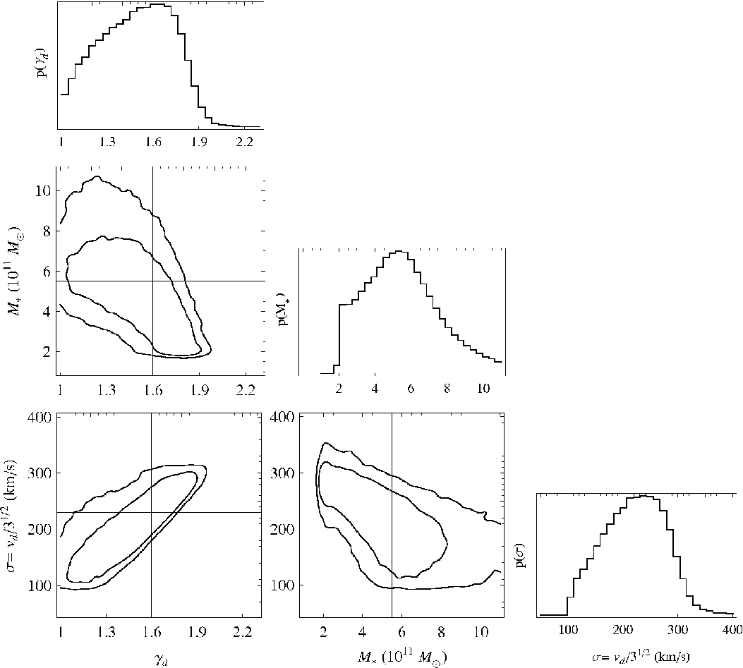
The virial theorem gives three velocity dispersions as a function of and the photometric parameters, which are used in the maximum likelihood method via eq. (8). Now the posterior distribution reproduces the same features of the model-independent partition, both in terms of effective radii () and velocity dispersions, which are listed in Table 5. Figure 7 shows the marginalised likelihood in terms of the dynamical parameters. Within this model, the posterior has a peak at and The confidence intervals for the parameters are: and Then, the underlying profile is reliably described as the superposition of simple luminous and dark components, although the inferred dynamical parameters inherit the large uncertainty from the photometric parameters. At very low values of the solution with and kms-1 is available. This conspiracy between luminous and dark matter to produce an overall profile has been observed in other cases (Treu & Koopmans, 2004; Humphrey & Buote, 2010; Remus et al., 2013),
Finally, it is interesting to compare the best-fitting dark matter masses to our earlier estimates in Table 4. Integrating our dark matter density law out to kpc, the dark matter mass is . Added to the luminous mass of gives a total mass of , reassuringly close to the value of given by the cruder estimates of Sect. 4.1. The total mass at kpc, inferred from the likelihood on the dynamical parameters, has sizeable uncertainties, namely
4.5 Evidence for DM Contraction
The model with luminous and dark components as in eq. (23) predicts kinematic and photometric properties compatible with the model-independent results of Section 3.2. At the same time, it yields information on the best fitting power-law slope of the dark matter. Although the posterior distribution of in Fig. 7 is broad, the peak of the distribution lies at . This suggests that the underlying DM density may be steeper than , which is predicted at small radii by cosmological DM-only simulations (Dubinski & Carlberg, 1991; Navarro et al., 1996, hereafter NFW). However, this result may be the outcome of a model, where the DM halo has a scale-free density. Perhaps the DM density is more appropriately described by a broken power-law similar to eq. (22), which is a simple generalisation of the NFW profile.
We can test whether this is a mere consequence of the adopted model by allowing the DM density to be a broken power-law, parameterized by an inner exponent a normalisation and a break-radius as in eq.(22). Within the virial method, we can use these as free parameters in the decomposition into three populations, provided the luminous mass is kept fixed. The procedure can be repeated for different fixed values of to quantify the change in the inferred and The posterior distribution (marginalised over colour and photometric parameters) has the same width regardless of the chosen value for whereas the maximum likelihood values vary as
| (25) | |||||
The uncertainties are symmetric for and and amount to and kms-1 respectively, whereas has a very skew posterior distribution around the peak value. We can marginalise the inner exponent over by considering a sum of Gaussians with mean and dispersion and weighing with the virial likelihood (Section 4.4 and Fig. 7). The resulting exponent is which is still appreciably different from the simple NFW prediction Furthermore, a decomposition relying strictly on a NFW halo gives inversions in the effective radii and velocities dispersions similarly to that found in Section 4.3. These findigs lend decisive support in favour of DM contraction, with a DM density exponent

5 Jeans analysis
In the previous sections, the dynamics of the system has been explored through the projected virial theorem, which is derived through integration of the Jeans equations over configuration space.
If instead the Jeans equations are employed directly, then the sub-populations are described by the previous parameters and also by their anisotropy profiles
| (26) |
Here, and are the radial and tangential velocity second moment, while is the spherical polar radius.
In our analysis, we will use
| (27) |
so that the inner anisotropy is and the outer anisotropy , whilst is a transition radius. Here, we use eq (16) of Paper I to calculate the velocity dispersions averaged within radial annuli, and thus build kinematic profiles, which are then used to separate the populations similarly to the procedure followed in the previous Sections.
As already noted in Section 3.2, the use of parameterised kinematic profiles, such as in eq (9), does not improve the inference on average velocity dispersions, which are linked to the mass model via the virial theorem. Thus, we can expect that the Jeans analysis will provide information on the velocity anisotropy profile, but no significant additional constraints on the mass model.
5.1 Dynamical parameters
The results of the previous sections suggest that we restrict attention to the two-component mass-model of eq. (23), which is both realistic (Section 4.4) and reliable (Section 4.5).
Once the likelihood is marginalised over the colour and photometric parameters, the posterior in the dynamical parameters and the anisotropies is left. In Fig. 8, we show the inference on the inner anisotropies of the three populations and on the dynamical parameters. The mass-anisotropy degeneracy is evident in the correlation between and the DM parameters for each population. There is a weaker correlation between this set of parameters and the remaining ones The posterior distribution of the dynamical parameters is similar to what we found in Section 4.4.
Compared to the virial results, the uncertainties on the DM parameters are slightly smaller but comparable. The likelihood profile is very shallow in and the marginalised posterior inherits its profile from the behaviour of the likelihood in the other parameters. For example, at small values of a wider range of anisotropies is allowed, giving a larger value for the integrated likelihood towards the low-mass end. This is another effect of the mass-anisotropy degeneracy. Having chosen a particular model for Jeans methods will privilege a narrower range of dynamical parameters, whereas the virial results account for the whole generality of anisotropy models that could be chosen.


5.2 Anisotropies
The inferences on outer anisotropies and anisotropy radii are shown in Fig. 9. The value of is not well constrained, the only reliable information being a lower limit (cf Sonnenfeld et al., 2012, for a similar case). A narrower distribution is obtained if the anisotropy at the effective radius is considered, which is shown in the last panel.
A glance at the inferred anisotropy profiles (figures 8 and 9) shows some interesting features of the system. The red GCs are on slightly tangential orbits, with nearly constant anisotropy. This may be simply consistent with the supposition that GCs at sufficiently small distances from M87 are tidally shredded at pericentric passage unless their orbits have sufficient angular momentum (Webb et al., 2013, cf). This creates a loss-cone (Bahcall & Wolf, 1976) in velocity space, whose aperture decreases with the distance from the center (as for a flat rotation curve). The intermediate-colour GCs, which orbit at larger radii, have a mildly radial anisotropy,
On the other hand, the blue GCs have approximately isotropic orbits at smaller radii and a mildly tangential velocity dispersion tensor at larger distances. This behaviour cannot be explained with arguments of tidal disruption, since the loss-cone in velocity space is already small enough for the intermediate-colour GCs to survive on mildly radial orbits. There is, however, another dynamical phenomenon that can produce such an anisotropy profile, which is related to the accretion process of the central object. If M87 has accreted mass on sufficiently slow time-scales, then radial orbits are dragged towards the center more efficiently than tangential ones (Goodman & Binney, 1984; Lee & Goodman, 1989; Cipollina & Bertin, 1994), which then contributes to a net tangential anisotropy in the outer parts. This scenario of (approximately) adiabatic contraction would also agree with the enhanced DM exponent, significantly larger than unity (Sections 4.4, 4.5).
Orbital time-scales are shorter at smaller distances. Then, if the intermediate-colour GCs are coeval with the blue ones, they must have experienced a similar phenomenon. The inferred positive value of for this population suggests that they have been falling onto M87 on preferentially radial orbits, differently from the more distant and bluer GCs.
6 Conclusions
The giant elliptical galaxy M87 is surrounded by one of the largest known populations of globular clusters (GCs), exceeding in total (Tamura et al., 2006). This extensive swarm of GCs offers a wealth of information regarding M87’s mass profile, together with tantalizing evidence about mechanisms of its formation and evolution. We have been able to answer some questions, thanks to the availability of a new data set of positions, colours and velocities with the largest radial extent and best kinematic accuracy to date (Strader et al 2011, or S11).
6.1 Multiple populations
The colour distribution and kinematics of the GCs at different radii suggest a partition into multiple sub-populations (see, for example, Harris 2009, S11 and references therein). Here, we have shown that a separation into three components is statistically preferred over ones into two or four populations for M87’s GC system. To separate the three components (blue, intermediate and red GCs), we have exploited a maximum-likelihood method in which the information from position, colour and velocity is used jointly. The average velocity dispersion and the colour-distribution parameters of each population are robustly determined, whereas the Sérsic indices and half-mass radii are affected by sizeable uncertainties (see for example, Table 2). The uncertainty in turn is a consequence of the limited number () of bona fide GCs with high quality spectroscopic data.
A case for more than two GC populations has been made also in studies of other galaxies, most notably NGC 4365 (Brodie et al., 2005). The same system has been reanalysed by Blom et al. (2012), where the colours of the three sub-populations have been linked to their different kinematics and viable formation scenarios. Here, we have shown how the dynamics (density profile and anisotropies) can be used, within a robust Bayesian analysis, to optimally decompose the GC system in sub-populations as well as compare formation scenarios with observational properties.
6.2 Masses

The kinematics of the GCs are a direct probe of the total mass distribution of M87. Each sub-population with its own global velocity dispersion and photometric parameters has its own virial pinch radius (eq.15,16 and Paper I). Therefore, the red, intermediate and blue GC populations provide us with three enclosed masses at three different pinch radii (see Table 4). The mass estimate at the pinch radius of the red GCs is corroborated by the results of more elaborate techniques applied to the stellar and GC populations (Murphy et al., 2011). The method is robust, as it is derived as a blind average over different possible halo mass models. The largest uncertainty is in the determination of the effective radius, and so the covariance between pinch radius and enclosed mass follows the scaling inherited from eq (15). This does not imply that the underlying mass distribution corresponds to that of a flat rotation curve. Indeed, there is a danger that the uncertainties scatter solutions along the locus of flat rotation curve models, which really amounts to fitting the covariance of the data rather than the underlying mass profile.
The mass profile can also be constrained by using dynamical modelling to obtain the velocity dispersions, which are then used to separate the three components. The first step consists of applying the Projected Virial Theorem (eq. 18). This has the advantage of involving the surface-density averaged (i.e. global) velocity dispersions only, thus avoiding systematic uncertainties arising from the mass-anisotropy degeneracy. By comparing the results of the separation relying on the virial theorem with those of the model-independent decomposition, we have been able to validate the luminous and dark matter model of eq (23), placing constraints on the luminous mass, dark matter (DM) density exponent and normalisation. The luminous and dark masses at different locations, together with their uncertainties, are discussed in Sections 4.1, 4.3 and 4.4. Figure 10 displays these results in terms of the inferred circular velocity at different locations.
The inferred density exponent is if a scale-free DM profile is used. When a broken power-law model for the DM halo is adopted, the inner exponent is still in the same range (). This is consistent with the findings of Sonnenfeld et al. (2012) for an early-type galaxy of similar mass and can be interpreted as evidence for DM contraction. The scale-radius arcsec where the DM density profile changes from to is somewhat smaller than the effective radius of the intermediate-colour population, but appreciably larger (or smaller) than the effective radius of the red (or blue) component.
6.3 Comparison with X-ray Studies
Studies in the literature compare the masses measured from the hot X-ray gas to those inferred from GC kinematics (Murphy et al., 2011). The X-ray masses are typically lower than the ones from GCs at small radii and larger at large radii. The discrepancy at small distances has been alleviated by invoking some amount of non-thermal support for the gas, but the disagreement at large distances would still hold (Humphrey et al., 2013). It is fair to say that previous studies relied on velocity dispersions that were appreciably overestimated, so the role of non-thermal motions is far from clear. The complex and asymmetric X-ray photometry of the gas calls for further caution in deriving masses from the X-ray gas based on assumptions such as spherical symmetry.
Another worry is the assumption that the gas is exactly in hydrostatic balance. If is the radial velocity of the gas, then from the Euler equation for a fluid flow with pressure and density
| (28) |
we see that depending on how the accreted gas settles towards hydrostatic equilibrium (i.e., positive or negative acceleration), the underlying mass profile may be under or over-estimated. This aspect has been discussed in detail for other systems (Ciotti & Pellegrini, 2004; Pellegrini & Ciotti, 2006), and there is evidence against hydrostatic equilibrium. Given the high virial mass of M87, it is plausible to assume that gas has been accreting onto it in the hot mode (Birnboim & Dekel, 2003), thus slowly setting towards hydrostatic balance after shocking at the virial radius. If the gas has bounced off the central regions, as a consequence of pressure build-up from the converging inflow, then it might be still experiencing a negative acceleration (from positive to zero velocity) and the mass from X-ray studies may be an underestimate. If at large distances the gas is still passing from negative to zero velocity, then the convective acceleration is positive and the X-ray mass may be an overestimate.
Das et al. (2010) found that the X-ray velocity curve of M87 rises from 500 km/s at 6 kpc (the effective radius of the starlight) to 600 km/s at large radii. They suggest that these numbers are susceptible to a 10 % uncertainty due to systematic effects. This takes them to values close to ours inferred from dynamical modelling, which range from 500 km/s at 6 kpc to 530 km/s at large radii. We conclude that there is tendency for the X-ray masses to be slightly overestimated at large radii, but that the discrepancy is within the uncertainties.
6.4 Orbits
The results from the Jeans analysis suggest an interesting distribution in velocity space. On the one hand, the GCs at small radii are consistent with a loss-cone distribution function that privileges tangential orbits, as GCs on radial orbits suffer tidal disruption near pericentric passage. On the other hand, at large distances the anisotropy profile of the blue GCs tends again towards mild tangentiality, which cannot be explained by loss-cone arguments. A more plausible scenario would invoke accretion of external material onto M87 once the GCs are already in place. The build-up of mass has a different effect on GC orbits depending on their angular momenta. If accretion proceeds slowly enough, this gives rise to a tangentially biased velocity-dispersion tensor in the outer parts, together with a contraction of the DM density profile at smaller distances.
Inference on the structure in velocity space has been possible within the framework of the simple analysis presented here. This is based on the Jeans equations and the approximation of spherical symmetry, which is appropriate as a first step in the case of M87. The use of more refined modelling techniques, such as non-spherical Jeans modelling, orbit-based or made-to-measure, would be useful to encode additional effects like possible flattening of the dark halo and more elaborate velocity distributions. However, the analysis of Amorisco & Evans (2012) and the sizeable statistical uncertainties on the surface-density parameters suggest that more advanced techniques will have to wait until larger data sets are collected.
Acknowledgments
We are indebted to Jay Strader for his observational effort on the M87 GC system, which has resulted in a sound basis for this work. We thank Luca Ciotti, Daniel Wang, Cathie Clarke and Andy Fabian for helpful discussions on X-ray masses, and Vasily Belokurov for significant feedback on the manuscript. We thank the anonymous referee for a very detailed report, which helped improve the manuscript considerably. AA acknowledges financial support from the Science and Technology Facilities Council (STFC) and the Isaac Newton Trust. AJR and JPB were supported by National Science Foundation grants AST-0909237 and AST-1211995.
References
- Abadi et al. (2010) Abadi, M. G., Navarro, J. F., Fardal, M., Babul, A., & Steinmetz, M. 2010, MNRAS, 407, 435
- Agnello & Evans (2012a) Agnello, A., & Evans, N. W. 2012a, MNRAS, 422, 1767
- Agnello & Evans (2012b) Agnello, A., & Evans, N. W. 2012b, ApJL, 754, L39
- Agnello et al. (2013) Agnello, A., Auger, M. W., & Evans, N. W. 2013, MNRAS, 429, L35
- Agnello et al. (2013b) Agnello, A., Evans, N. W. 2013, MNRAS, submitted (Paper I)
- Amorisco & Evans (2011) Amorisco, N. C., & Evans, N. W., 2011, MNRAS, 411, 2118
- Amorisco & Evans (2012) Amorisco, N. C., & Evans, N. W. 2012, MNRAS, 424, 1899
- Amorisco et al. (2013) Amorisco, N. C., Agnello, A., & Evans, N. W. 2013, MNRAS, 429, L89
- Bahcall & Wolf (1976) Bahcall, J. N., & Wolf, R. A. 1976, ApJ, 209, 214
- Bird et al. (2010) Bird, S., Harris, W.E., Blakeslee, J.P., Flynn, C. 2010, AA, 524, A71
- Birnboim & Dekel (2003) Birnboim Y., Dekel, A. 2003. MNRAS, 345, 349
- Blom et al. (2012) Blom, C., Forbes, D. A., Brodie, J. P., et al. 2012, MNRAS, 426, 1959
- Blumenthal et al. (1986) Blumenthal, G. R., Faber, S. M., Flores, R.,& Primack, J. R. 1986, ApJ, 301, 27
- Brodie et al. (2005) Brodie, J. P., Strader, J., Denicoló, G., et al. 2005, AJ, 129, 2643
- Brodie & Strader (2006) Brodie, J. P., & Strader, J. 2006, ARA&A, 44, 193
- Brodie et al. (2011) Brodie, J. P., Romanowsky, A. J., Strader, J., & Forbes, D. A. 2011, AJ, 142, 199
- Burnham & Anderson (2002) Burnham, K. P., Anderson, D. R. 2002, Model Selection and Multimodel Inference; Springer, 2nd ed.
- Cappellari et al. (2006) Cappellari, M., Bacon, R., Bureau, M., et al. 2006, MNRAS, 366, 1126
- Churazov et al. (2010) Churazov, E., Tremaine, S., Forman, W., et al. 2010, MNRAS, 404, 1165
- Ciotti & Bertin (1999) Ciotti, L., & Bertin, G. 1999, AA, 352, 447
- Ciotti & Pellegrini (2004) Ciotti, L., & Pellegrini, S. 2004, MNRAS, 350, 609
- Pellegrini & Ciotti (2006) Pellegrini, S., & Ciotti, L. 2006, MNRAS, 370, 1797
- Cipollina & Bertin (1994) Cipolina, M., Bertin, G., 1994, AA, 288, 43
- Coccato et al. (2009) Coccato, L., Gerhard, O., Arnaboldi, M., et al. 2009, MNRAS, 394, 1249
- Cohen & Ryzhov (1997) Cohen, J. G., & Ryzhov, A. 1997, ApJ, 486, 230
- Cohen (2000) Cohen, J. G. 2000, AJ, 119, 162
- Das et al. (2010) Das, P., Gerhard, O., Churazov, E., & Zhuravleva, I. 2010, MNRAS, 409, 1362
- Deason et al. (2012) Deason, A. J., Belokurov, V., Evans, N. W., & McCarthy, I. G. 2012, ApJ, 748, 2
- Dekel et al. (2005) Dekel, A., Stoehr, F., Mamon, G. A., et al. 2005, Nat, 437, 707
- Douglas et al. (2002) Douglas, N. G., Arnaboldi, M., Freeman, K. C., et al. 2002, PASP, 114, 1234
- Dubinski & Carlberg (1991) Dubinski, J., & Carlberg, R. G. 1991, ApJ, 378, 496
- Goodman & Binney (1984) Goodman, J., & Binney, J.J. 1984, MNRAS, 207,511
- Hanes et al. (2001) Hanes, D. A., Côté, P., Bridges, T. J., et al. 2001, ApJ, 559, 812
- Harris (2009) Harris, W. E. 2009, ApJ, 703, 939
- Hilz et al. (2013) Hilz, M., Naab, T.,& Ostriker, J. P. 2013, MNRAS, 429, 2924
- Huchra & Brodie (1987) Huchra, J., & Brodie, J. 1987, AJ, 93, 779
- Humphrey & Buote (2010) Humphrey, P.J., Buote, D. 2010, MNRAS, 403, 2143
- Humphrey et al. (2013) Humphrey, P. J., Buote, D. A., Brighenti, F., Gebhardt, K., & Mathews, W. G. 2013, MNRAS, 430, 1516
- Jaffe (1983) Jaffe, W. 1983, MNRAS, 202, 995
- Janowiecki et al. (2010) Janowiecki, S., Mihos, J. C., Harding, P., et al. 2010, ApJ, 715, 972
- Jeffreys (1961) Jeffreys, H., 1961, The Theory of Probability, Oxford University Press
- Johansson et al . (2012) Johansson, P. H.., Naab, T., & Ostriker, J. P. 2012, ApJ, 754, 115
- Jorgensen et al. (1995) Jorgensen, I., Franx, M., & Kjaergaard, P. 1995, MNRAS, 273, 1097
- Kendall & Stuart (1979) Kendall, M., & Stuart, A. 1979, London: Griffin, 1979, 4th ed.
- Lee & Goodman (1989) Lee, M. H., Goodman, J. 1989, ApJ, 343, 594
- Madrid et al. (2009) Madrid J.P., Harris W.E., Blakeslee J.P., Gomez, M. 2009, ApJ, 7905, 237
- McLaughlin (1999) McLaughlin, D. E. 1999, ApJL, 512, L9
- Morganti et al. (2013) Morganti, L., Gerhard, O., Coccato, L., Martinez-Valpuesta, I., & Arnaboldi, M. 2013, MNRAS, 431, 3570
- Mould et al. (1987) Mould, J. R., Oke, J. B., & Nemec, J. M. 1987, AJ, 93, 53
- Mould et al. (1990) Mould, J. R., Oke, J. B., de Zeeuw, P. T., & Nemec, J. M. 1990, AJ, 99, 1823
- Murphy et al. (2011) Murphy, J. D., Gebhardt, K., & Adams, J. J. 2011, ApJ, 729, 129
- Napolitano et al. (2009) Napolitano, N. R., Romanowsky, A. J., Coccato, L., et al. 2009, MNRAS, 393, 329
- Navarro et al. (1996) Navarro, J., Frenk, C.S., White, S.D.M. 1996, ApJ, 462, 563
- Nipoti et al. (2012) Nipoti, C., Treu, T., Leauthaud, A., et al. 2012, MNRAS, 422, 1714
- Pota et al. (2013) Pota, V., Forbes, D. A., Romanowsky, A. J., et al. 2013, MNRAS, 428, 389
- Remus et al. (2013) Remus, R.-S., Burkert, A., Dolag, K., et al. 2013, ApJ, 766, 71
- Richardson & Fairbairn (2013) Richardson, T., & Fairbairn, M. 2013, arXiv:1305.0670
- Romanowsky & Kochanek (2001) Romanowsky, A. J., & Kochanek, C. S. 2001, ApJ, 553, 722
- Romanowsky et al. (2003) Romanowsky, A. J., Douglas, N. G., Arnaboldi, M., et al. 2003, Science, 301, 1696
- Romanowsky et al. (2012) Romanowsky, A. J., Strader, J., Brodie, J. P., et al. 2012, ApJ, 748, 29
- Schwarzschild (1979) Schwarzschild, M. 1979, ApJ, 232, 236
- Schuberth et al. (2010) Schuberth, Y., Richtler, T., Hilker, M., et al. 2010, AA, 513, A52
- Schuberth et al. (2012) Schuberth, Y., Richtler, T., Hilker, M., et al. 2012, AA, 544, A115
- Sonnenfeld et al. (2012) Sonnenfeld, A., Treu, T., Gavazzi, R., Marshall, P.J., Auger, M.W., Suyu, S.H., Koopmans, L.V.E., Bolton, A.S. 2012, ApJ, 752, 163
- Strader et al. (2011) Strader, J., Romanowsky, A. J., Brodie, J. P., et al. 2011, ApJS, 197, 33
- Stiavelli & Bertin (1987) Stiavelli, M., & Bertin, G. 1987, MNRAS, 229, 61
- Syer & Tremaine (1996) Syer, D., & Tremaine, S. 1996, MNRAS, 282, 223
- Tamura et al. (2006) Tamura, N., Sharples, R. M., Arimoto, N., et al. 2006, MNRAS, 373, 588
- Tortora et al. (2009) Tortora, C., Napolitano, N. R., Romanowsky, A. J., Capaccioli, M., & Covone, G. 2009, MNRAS, 396, 1132
- Treu & Koopmans (2004) Treu, T., & Koopmans, L. V. E. 2004, ApJ, 611, 739
- Walker & Peñarrubia (2011) Walker, M. G., & Peñarrubia, J. 2011, ApJ, 742, 20
- Watkins et al. (2010) Watkins, L. L., Evans, N. W., & An, J. H. 2010, MNRAS, 406, 264
- Webb et al. (2013) Webb, J. J., Harris, W. E., Sills, A., & Hurley, J. R. 2013, ApJ, 764, 124
- Wu & Tremaine (2006) Wu, X., & Tremaine, S. 2006, ApJ, 643, 210
- Zubovas & King (2012) Zubovas, K., & King, A. R. 2012, MNRAS, 426, 2751