跳到论文正文
W Papers独立论文阅读器 arXiv:1401.4425 论文正文 计算阅读时间 · 0%
引用这篇论文根据当前论文元数据生成,正式投稿前建议核对。


License: arXiv.org perpetual non-exclusive license
arXiv:1401.4425v2 [stat.ME] 13 Jul 2014

Monte Carlo Simulation for Lasso-Type Problems
by Estimator Augmentation

Qing Zhou ††thanks: UCLA Department of Statistics (email: zhou@stat.ucla.edu). This work was supported by NSF grants DMS-1055286 and DMS-1308376. The author thanks one referee for providing useful references.
Abstract

Regularized linear regression under the ℓ1\ell_{1} penalty, such as the Lasso, has been shown to be effective in variable selection and sparse modeling. The sampling distribution of an ℓ1\ell_{1}-penalized estimator 𝜷^\hat{\bm{\beta}} is hard to determine as the estimator is defined by an optimization problem that in general can only be solved numerically and many of its components may be exactly zero. Let 𝐒\mathbf{S} be the subgradient of the ℓ1\ell_{1} norm of the coefficient vector 𝜷\bm{\beta} evaluated at 𝜷^\hat{\bm{\beta}}. We find that the joint sampling distribution of 𝜷^\hat{\bm{\beta}} and 𝐒\mathbf{S}, together called an augmented estimator, is much more tractable and has a closed-form density under a normal error distribution in both low-dimensional (p≤np\leq n) and high-dimensional (p>np>n) settings. Given 𝜷\bm{\beta} and the error variance σ2\sigma^{2}, one may employ standard Monte Carlo methods, such as Markov chain Monte Carlo and importance sampling, to draw samples from the distribution of the augmented estimator and calculate expectations with respect to the sampling distribution of 𝜷^\hat{\bm{\beta}}. We develop a few concrete Monte Carlo algorithms and demonstrate with numerical examples that our approach may offer huge advantages and great flexibility in studying sampling distributions in ℓ1\ell_{1}-penalized linear regression. We also establish nonasymptotic bounds on the difference between the true sampling distribution of 𝜷^\hat{\bm{\beta}} and its estimator obtained by plugging in estimated parameters, which justifies the validity of Monte Carlo simulation from an estimated sampling distribution even when p≫n→∞p\gg n\to\infty.

Key words: Confidence interval, importance sampling, Lasso, Markov chain Monte Carlo, p-value, sampling distribution, sparse linear model.

1 Introduction

Consider the linear regression model,

𝐲=𝐗​𝜷+𝜺,\mathbf{y}=\mathbf{X}\bm{\beta}+\bm{\varepsilon}, (1.1)

where 𝐲\mathbf{y} is an nn-vector, 𝐗\mathbf{X} an n×pn\times p design matrix, 𝜷=(βj)1:p\bm{\beta}=(\beta_{j})_{1:p} the vector of coefficients, and 𝜺\bm{\varepsilon} i.i.d. random errors with mean zero and variance σ2\sigma^{2}. Recently, ℓ1\ell_{1}-penalized estimation methods (Tibshirani 1996; Chen et al. 1999) have been widely used to find sparse estimates of the coefficient vector. Given positive weights wjw_{j}, j=1,…,pj=1,\ldots,p, and a tuning parameter λ>0\lambda>0, an ℓ1\ell_{1}-penalized estimator 𝜷^=(β^j)1:p\hat{\bm{\beta}}=(\hat{\beta}_{j})_{1:p} is defined by minimizing the following penalized loss function,

ℓ⁡(𝜷)=12​‖𝐲−𝐗​𝜷‖22+n​λ​∑j=1pwj​|βj|.\ell(\bm{\beta})=\frac{1}{2}\|\mathbf{y}-\mathbf{X}\bm{\beta}\|_{2}^{2}+n\lambda\sum_{j=1}^{p}w_{j}|\beta_{j}|. (1.2)

By different ways of choosing wjw_{j}, the estimator corresponds to the Lasso (Tibshirani 1996), the adaptive Lasso (Zou 2006), and the one-step linear local approximation (LLA) estimator (Zou and Li 2008) among others. We call such an estimator a Lasso-type estimator.

In many applications of ℓ1\ell_{1}-penalized regression, it is desired to quantify the uncertainty in the estimates. However, except for very special cases, the sampling distribution of a Lasso-type estimator is complicated and difficult to approximate. Closed-form approximations to the covariance matrices of the estimators in Tibshirani (1996), Fan and Li (2001), and Zou (2006) are unsatisfactory, as they all give zero variance for a zero component of the estimators and thus fail to quantify the uncertainty in variable selection. Theoretical results on finite-sample distributions and confidence sets of some Lasso-type estimators have been developed (Pötscher and Schneider 2009; Pötscher and Schneider 2010) but only under orthogonal designs, which clearly limits general applications of these results. The bootstrap can be used to approximate the sampling distribution of a Lasso-type estimator, in which numerical optimization is needed to minimize (1.2) for every bootstrap sample. Although there are efficient algorithms, such as the Lars (Efron et al. 2004), the homotopy algorithm (Osborne et al. 2000), and coordinate descent (Friedman et al. 2007; Wu and Lange 2008), to solve this optimization problem, it is still time-consuming to apply these algorithms hundreds or even thousands of times in bootstrap sampling. As pointed out by Knight and Fu (2000) and Chatterjee and Lahiri (2010), the bootstrap may not be consistent for estimating the sampling distribution of the Lasso under certain circumstances. To overcome this difficulty, a modified bootstrap (Chatterjee and Lahiri 2011) and a perturbation resampling approach (Minnier et al. 2011) have been proposed, both justified under a fixed-pp asymptotic framework. Zhang and Zhang (2014) have developed methods for constructing confidence intervals for individual coefficients and their linear combinations in high-dimensional (p>np>n) regression with sufficient conditions for the asymptotic normality of the proposed estimators. There are several recent articles on significance test and confidence region construction for sparse high-dimensional linear models (Javanmard and Montanari 2013a; Javanmard and Montanari 2013b; Lockhart et al. 2014; van de Geer et al. 2013), all based on asymptotic distributions for various functions of the Lasso. On the other hand, knowledge on sampling distributions is also useful for distribution-based model selection with ℓ1\ell_{1} penalization, as demonstrated by stability selection (Meinshausen and Bühlmann 2010) and the Bolasso (Bach 2008).

A possible alternative to the bootstrap or resampling is to simulate from a sampling distribution by Monte Carlo methods, such as Markov chain Monte Carlo (MCMC). An obvious obstacle to using these methods for a Lasso-type estimator is that its sampling distribution does not have a closed-form density. In this article, we study the joint distribution of a Lasso-type estimator 𝜷^\hat{\bm{\beta}} and the subgradient 𝐒\mathbf{S} of ‖𝜷‖1\|\bm{\beta}\|_{1} evaluated at 𝜷^\hat{\bm{\beta}}. Interestingly, this joint distribution has a density that can be calculated explicitly assuming a normal error distribution, regardless of the relative size between nn and pp. Thus, one can develop Monte Carlo algorithms to draw samples from this joint distribution and estimate various expectations of interest with respect to the sampling distribution of 𝜷^\hat{\bm{\beta}}, which is simply a marginal distribution. This approach offers great flexibility in studying the sampling distribution of a Lasso-type estimator. For instance, one may use importance sampling (IS) to accurately estimate a tail probability (small p-value) with respect to the sampling distribution under a null hypothesis, which can be orders of magnitude more efficient than any method directly targeting at the sampling distribution. Another potential advantage of this approach is that, at each iteration, an MCMC algorithm only evaluates a closed-form density, which is much faster than minimizing (1.2) numerically as used in the bootstrap. Furthermore, our method can be interpreted as an MCMC algorithm targeting at a multivariate normal distribution with locally reparameterized moves and hence is expected to be computationally tractable.

The remaining part of this article is organized as follows. After a high-level description of the basic idea, Section 2 derives the density of the joint distribution of 𝜷^\hat{\bm{\beta}} and 𝐒\mathbf{S} in the low-dimensional setting with p≤np\leq n, and Section 3 develops MCMC algorithms for this setting. The density in the high-dimensional setting with p>np>n is derived in Section 4. In Section 5, we construct applications of the high-dimensional result in p-value calculation for Lasso-type inference by IS. Numerical examples are provided in Sections 3 and 5 to demonstrate the efficiency of the Monte Carlo algorithms. Section 6 provides theoretical justifications for simulation from an estimated sampling distribution of the Lasso by establishing its consistency as p≫n→∞p\gg n\to\infty. Section 7 includes generalizations to random designs, a connection to model selection consistency, and a Bayesian interpretation of the sampling distribution. The article concludes with a brief discussion and some remarks. Technical proofs are relegated to Section 8.

Notations for vectors and matrices are defined here. All vectors are regarded as column vectors. Let A={j1,…,jk}⊆{1,…,m}A=\{j_{1},\ldots,j_{k}\}\subseteq\{1,\ldots,m\} and B={i1,…,iℓ}⊆{1,…,n}B=\{i_{1},\ldots,i_{\ell}\}\subseteq\{1,\ldots,n\} be two index sets. For vectors 𝐯=(vj)1:m\mathbf{v}=(v_{j})_{1:m} and 𝐮=(ui)1:n\mathbf{u}=(u_{i})_{1:n}, we define 𝐯A=(vj)j∈A=(vj1,…,vjk)\mathbf{v}_{A}=(v_{j})_{j\in A}=(v_{j_{1}},\ldots,v_{j_{k}}), 𝐯−A=(vj)j∉A\mathbf{v}_{-A}=(v_{j})_{j\notin A}, and (𝐯A,𝐮B)=(vj1,…,vjk,ui1,…,uiℓ)(\mathbf{v}_{A},\mathbf{u}_{B})=(v_{j_{1}},\ldots,v_{j_{k}},u_{i_{1}},\ldots,u_{i_{\ell}}). For a matrix 𝐌=(Mi​j)m×n\mathbf{M}=(M_{ij})_{m\times n}, write its columns as 𝐌j\mathbf{M}_{j}, j=1,…,nj=1,\ldots,n. Then 𝐌B=(𝐌j)j∈B\mathbf{M}_{B}=(\mathbf{M}_{j})_{j\in B} extracts the columns in BB, the submatrix 𝐌A​B=(Mi​j)i∈A,j∈B\mathbf{M}_{AB}=(M_{ij})_{i\in A,j\in B} extracts the rows in AA and the columns in BB, and 𝐌A∙=(Mi​j)i∈A\mathbf{M}_{A\bullet}=(M_{ij})_{i\in A} extracts the rows in AA. Furthermore, 𝐌B𝖳\mathbf{M}^{\mathsf{T}}_{B} and 𝐌A​B𝖳\mathbf{M}_{AB}^{\mathsf{T}} are understood as (𝐌B)𝖳(\mathbf{M}_{B})^{\mathsf{T}} and (𝐌A​B)𝖳(\mathbf{M}_{AB})^{\mathsf{T}}, respectively. We denote the row space, the null space, and the rank of 𝐌\mathbf{M} by row​(𝐌)\text{row}(\mathbf{M}), null​(𝐌)\text{null}(\mathbf{M}), and rank​(𝐌)\text{rank}(\mathbf{M}), respectively. Denote by diag​(𝐯)\mbox{diag}(\mathbf{v}) the m×mm\times m diagonal matrix with 𝐯\mathbf{v} as the diagonal elements, and by diag​(𝐌,𝐌′)\mbox{diag}(\mathbf{M},\mathbf{M}^{\prime}) the block diagonal matrix with 𝐌\mathbf{M} and 𝐌′\mathbf{M}^{\prime} as the diagonal blocks, where the submatrices 𝐌\mathbf{M} and 𝐌′\mathbf{M}^{\prime} may be of different sizes and may not be square. For a square matrix 𝐌\mathbf{M}, diag​(𝐌)\mbox{diag}(\mathbf{M}) extracts the diagonal elements. Denote by 𝐈n\mathbf{I}_{n} the n×nn\times n identity matrix.

2 Estimator augmentation

2.1 The basic idea

Let 𝐖=diag​(w1,…,wp)\mathbf{W}=\mbox{diag}(w_{1},\ldots,w_{p}). A minimizer 𝜷^\hat{\bm{\beta}} of (1.2) is given by the Karush-Kuhn-Tucker (KKT) condition

1n​𝐗𝖳​𝐲=1n​𝐗𝖳​𝐗​𝜷^+λ​𝐖𝐒,\frac{1}{n}\mathbf{X}^{\mathsf{T}}\mathbf{y}=\frac{1}{n}\mathbf{X}^{\mathsf{T}}\mathbf{X}\hat{\bm{\beta}}+\lambda\mathbf{W}\mathbf{S}, (2.1)

where 𝐒=(Sj)1:p\mathbf{S}=(S_{j})_{1:p} is the subgradient of the function g⁡(𝜷)=‖𝜷‖1g(\bm{\beta})=\|\bm{\beta}\|_{1} evaluated at the solution 𝜷^\hat{\bm{\beta}}. Therefore,

{Sj=sgn​(β^j) if ​β^j≠0,Sj∈[−1,1] if ​β^j=0,\left\{\begin{array}[]{ll}S_{j}=\mbox{sgn}(\hat{\beta}_{j})&\mbox{ if }\hat{\beta}_{j}\neq 0,\\ S_{j}\in[-1,1]&\mbox{ if }\hat{\beta}_{j}=0,\end{array}\right. (2.2)

for j=1,…,pj=1,\ldots,p. Hereafter, we may simply call 𝐒\mathbf{S} the subgradient if the meaning is clear from context. Lemma 1 reviews a few basic facts about the uniqueness of 𝜷^\hat{\bm{\beta}} and 𝐒\mathbf{S}.

Lemma 1.

For any 𝐲\mathbf{y}, 𝐗\mathbf{X} and λ>0\lambda>0, every minimizer 𝜷^\hat{\bm{\beta}} of (1.2) gives the same fitted value 𝐗​𝜷^\mathbf{X}\hat{\bm{\beta}} and the same subgradient 𝐒\mathbf{S}. Moreover, if the columns of 𝐗\mathbf{X} are in general position, then 𝜷^\hat{\bm{\beta}} is unique for any 𝐲\mathbf{y} and λ>0\lambda>0.

Proof.

See Lemma 1 and Lemma 3 in Tibshirani (2013) for proof of the uniqueness of the fitted value 𝐗​𝜷^\mathbf{X}\hat{\bm{\beta}} and the uniqueness of 𝜷^\hat{\bm{\beta}}. Since 𝐒\mathbf{S} is a (vector-valued) function of 𝐗​𝜷^\mathbf{X}\hat{\bm{\beta}} from the KKT condition (2.1), it is also unique for fixed 𝐲\mathbf{y}, 𝐗\mathbf{X} and λ\lambda. ∎

We regard 𝜷^\hat{\bm{\beta}} and 𝐒\mathbf{S} together as the solution to Equation (2.1). Lemma 1 establishes that (𝜷^,𝐒)(\hat{\bm{\beta}},\mathbf{S}) is unique for any 𝐲\mathbf{y} assuming the columns of 𝐗\mathbf{X} are in general position (for a technical definition see Tibshirani 2013), regardless of the sizes of nn and pp. We call the vector (𝜷^,𝐒)(\hat{\bm{\beta}},\mathbf{S}) the augmented estimator in an ℓ1\ell_{1}-penalized regression problem. The augmented estimator will play a central role in our study of the sampling distribution of 𝜷^\hat{\bm{\beta}}.

Let 𝐔=1n​𝐗𝖳​𝜺=1n​𝐗𝖳​𝐲−𝐂​𝜷\mathbf{U}=\frac{1}{n}\mathbf{X}^{\mathsf{T}}\bm{\varepsilon}=\frac{1}{n}\mathbf{X}^{\mathsf{T}}\mathbf{y}-\mathbf{C}\bm{\beta}, where 𝐂=1n​𝐗𝖳​𝐗\mathbf{C}=\frac{1}{n}\mathbf{X}^{\mathsf{T}}\mathbf{X} is the Gram matrix. By definition, 𝐔∈row​(𝐗)\mathbf{U}\in\text{row}(\mathbf{X}). Rewrite the KKT condition as

𝐔=𝐂​𝜷^+λ​𝐖𝐒−𝐂​𝜷​=Δ𝐇⁡(𝜷^,𝐒,𝜷),\mathbf{U}=\mathbf{C}\hat{\bm{\beta}}+\lambda\mathbf{W}\mathbf{S}-\mathbf{C}\bm{\beta}\mathop{=}\limits^{\Delta}\mathbf{H}(\hat{\bm{\beta}},\mathbf{S};\bm{\beta}), (2.3)

which shows that 𝐔\mathbf{U} is a function of (𝜷^,𝐒)(\hat{\bm{\beta}},\mathbf{S}). On the other hand, 𝐲\mathbf{y} determines (𝜷^,𝐒)(\hat{\bm{\beta}},\mathbf{S}) only through 𝐔\mathbf{U}, which implies that (𝜷^,𝐒)(\hat{\bm{\beta}},\mathbf{S}) is unique for any 𝐔\mathbf{U} as long as it is unique for any 𝐲\mathbf{y}. Therefore, under the assumptions for the uniqueness of 𝜷^\hat{\bm{\beta}}, 𝐇\mathbf{H} is a bijection between (𝜷^,𝐒)(\hat{\bm{\beta}},\mathbf{S}) and 𝐔\mathbf{U}. For a fixed 𝐗\mathbf{X}, the only source of randomness in the linear model (1.1) is the noise vector 𝜺\bm{\varepsilon}, which determines the distribution of 𝐔\mathbf{U}. With the bijection between 𝐔\mathbf{U} and (𝜷^,𝐒)(\hat{\bm{\beta}},\mathbf{S}), one may derive the joint distribution of (𝜷^,𝐒)(\hat{\bm{\beta}},\mathbf{S}), which has a closed-form density under a normal error distribution. Then we develop Monte Carlo algorithms to sample from this joint distribution and obtain the sampling distribution of 𝜷^\hat{\bm{\beta}}. This is the key idea of this article, which works for both the low-dimensional setting (p≤np\leq n) and the high-dimensional setting (p>np>n). Although the basic strategy is the same, the technical details are slightly more complicated for the high-dimensional setting. For the sake of understanding, we first focus on the low-dimensional case in the remaining part of Section 2 and Section 3, and then generalize the results to the high-dimensional setting in Section 4.

Before going through all the technical details, we take a glimpse of the utility of this work in a couple concrete examples. Given a design matrix 𝐗\mathbf{X} and a value of λ\lambda, our method gives a closed-form joint density π\pi for the Lasso-type estimator 𝜷^\hat{\bm{\beta}} and the subgradient 𝐒\mathbf{S} under assumed values of the true parameters (Theorems 1 and 2). Targeting at this density, we have developed MCMC algorithms, such as the Lasso sampler in Section 3.2, to draw samples from the joint distribution of (𝜷^,𝐒)(\hat{\bm{\beta}},\mathbf{S}). Such MCMC samples allow for approximation of marginal distributions for a Lasso-type estimator. Figure 1 demonstrates the results of the Lasso sampler applied on a simulated dataset with n=500n=500, p=100p=100 and a normal error distribution. The scatter plot in Figure 1(a) confirms that β^j\hat{\beta}_{j} indeed may have a positive probability to be exactly zero in its sampling distribution. Accordingly, the distribution of the subgradient SjS_{j} in Figure 1(b) has a continuous density on (−1,1)(-1,1) and two point masses on ±1\pm 1. The fast mixing and low autocorrelation shown in the figure are surprisingly satisfactory for a simple MCMC algorithm in such a high-dimensional and complicated space (ℝp×2{1,…,p}\mathbb{R}^{p}\times 2^{\{1,\ldots,p\}}, see (2.4)). Exploiting the explicit form of the bijection 𝐇\mathbf{H}, we achieve the goal of sampling from the joint distribution of (𝜷^,𝐒)(\hat{\bm{\beta}},\mathbf{S}) via an MCMC algorithm essentially targeting at a multivariate normal distribution (Section 3.5). This approach does not need numerical optimization in any step, which makes it highly efficient compared to bootstrap or resampling-based methods. Another huge potential of our method is its ability to estimate tail probabilities, such as small p-values in a significance test (Section 5). Estimating tail probabilities is challenging for any simulation method. With a suitable proposal distribution, having an explicit density makes it possible to accurately estimate tail probabilities by importance weights. For example, our method can estimate a tail probability on the order of 10−2010^{-20}, with a coefficient of variation around 2, by simulating only 5,000 samples from a proposal distribution. This is absolutely impossible when bootstrapping the Lasso or simulating from the sampling distribution directly.

Refer to caption

(a)

Refer to caption

(b)

Refer to caption

(c)

Refer to caption

(d)

Figure 1: Demonstration of the Lasso sampler on a dataset with p=100p=100. (a) Scatter plot of the samples of β^1\hat{\beta}_{1} (x-axis) and β^50\hat{\beta}_{50} (y-axis); (b) histogram of the subgradient S50S_{50}; (c) two sample paths of β^1\hat{\beta}_{1} with diverse initial values; (d) a typical autocorrelation function.

2.2 The bijection

In the low-dimensional setting, we assume that rank​(𝐗)=p≤n\text{rank}(\mathbf{X})=p\leq n, which guarantees that the columns of 𝐗\mathbf{X} are in general position.

Before writing down the bijection explicitly, we first examine the respective spaces for 𝐔\mathbf{U} and (𝜷^,𝐒)(\hat{\bm{\beta}},\mathbf{S}). Under the assumption that rank​(𝐗)=p\text{rank}(\mathbf{X})=p, the row space of 𝐗\mathbf{X} is simply ℝp\mathbb{R}^{p}, which is the space for 𝐔\mathbf{U}. Let 𝒜=supp​(𝜷^)​=Δ{j:β^j≠0}\mathcal{A}=\text{supp}(\hat{\bm{\beta}})\mathop{=}\limits^{\Delta}\{j:\hat{\beta}_{j}\neq 0\} be the active set of 𝜷^\hat{\bm{\beta}} and ℐ={1,…,p}∖𝒜\mathcal{I}=\{1,\ldots,p\}\setminus\mathcal{A} be the inactive set, i.e., the set of the zero components of 𝜷^\hat{\bm{\beta}}. After removing the degeneracies among its components as given in (2.2), the vector (𝜷^,𝐒)(\hat{\bm{\beta}},\mathbf{S}) can be equivalently represented by the triple (𝜷^𝒜,𝐒ℐ,𝒜)(\hat{\bm{\beta}}_{\mathcal{A}},\mathbf{S}_{\mathcal{I}},\mathcal{A}). They are equivalent because from (𝜷^𝒜,𝐒ℐ,𝒜)(\hat{\bm{\beta}}_{\mathcal{A}},\mathbf{S}_{\mathcal{I}},\mathcal{A}) one can unambiguously recover (𝜷^,𝐒)(\hat{\bm{\beta}},\mathbf{S}), by setting 𝜷^ℐ=𝟎\hat{\bm{\beta}}_{\mathcal{I}}=\mathbf{0} and 𝐒𝒜=sgn​(𝜷^𝒜)\mathbf{S}_{\mathcal{A}}=\mbox{sgn}(\hat{\bm{\beta}}_{\mathcal{A}}) (2.2), and vice versa. It is more convenient and transparent to work with this equivalent representation. One sees immediately that (𝜷^𝒜,𝐒ℐ,𝒜)(\hat{\bm{\beta}}_{\mathcal{A}},\mathbf{S}_{\mathcal{I}},\mathcal{A}) lies in

Ω={(𝐛A,𝐬I,A):A⊆{1,…,p},𝐛A∈(ℝ∖{0})|A|,𝐬I∈[−1,1]p−|A|},\Omega=\{(\mathbf{b}_{A},\mathbf{s}_{I},A):A\subseteq\{1,\ldots,p\},\mathbf{b}_{A}\in(\mathbb{R}\setminus\{0\})^{|A|},\mathbf{s}_{I}\in[-1,1]^{p-|A|}\}, (2.4)

where I={1,…,p}∖AI=\{1,\ldots,p\}\setminus A. Hereafter, we always understand (𝐛A,𝐬I,A)(\mathbf{b}_{A},\mathbf{s}_{I},A) as the equivalent representation of (𝐛,𝐬)=((bj)1:p,(sj)1:p)(\mathbf{b},\mathbf{s})=((b_{j})_{1:p},(s_{j})_{1:p}) with supp​(𝐛)=A\text{supp}(\mathbf{b})=A and 𝐬A=sgn​(𝐛A)\mathbf{s}_{A}=\mbox{sgn}(\mathbf{b}_{A}). Clearly, Ω⊂ℝp×2{1,…,p}\Omega\subset\mathbb{R}^{p}\times 2^{\{1,\ldots,p\}}, where 2{1,…,p}2^{\{1,\ldots,p\}} is the collection of all subsets of {1,…,p}\{1,\ldots,p\}, and thus (𝜷^𝒜,𝐒ℐ,𝒜)(\hat{\bm{\beta}}_{\mathcal{A}},\mathbf{S}_{\mathcal{I}},\mathcal{A}) lives in the product space of ℝp\mathbb{R}^{p} and a finite discrete space.

Partition 𝜷^\hat{\bm{\beta}} as (𝜷^𝒜,𝜷^ℐ)=(𝜷^𝒜,𝟎)(\hat{\bm{\beta}}_{\mathcal{A}},\hat{\bm{\beta}}_{\mathcal{I}})=(\hat{\bm{\beta}}_{\mathcal{A}},\mathbf{0}) and 𝐒\mathbf{S} as (𝐒𝒜,𝐒ℐ)=(sgn​(𝜷^𝒜),𝐒ℐ)(\mathbf{S}_{\mathcal{A}},\mathbf{S}_{\mathcal{I}})=(\mbox{sgn}(\hat{\bm{\beta}}_{\mathcal{A}}),\mathbf{S}_{\mathcal{I}}). Then the KKT condition (2.3) can be rewritten,

𝐔\displaystyle\mathbf{U} =\displaystyle= (𝐂𝒜∣𝐂ℐ)​(𝜷^𝒜𝟎)+λ⁡(𝐖𝒜∣𝐖ℐ)​(𝐒𝒜𝐒ℐ)−𝐂​𝜷,\displaystyle(\mathbf{C}_{\mathcal{A}}\mid\mathbf{C}_{\mathcal{I}})\left(\begin{array}[]{c}\hat{\bm{\beta}}_{\mathcal{A}}\\ \mathbf{0}\\ \end{array}\right)+\lambda(\mathbf{W}_{\mathcal{A}}\mid\mathbf{W}_{\mathcal{I}})\left(\begin{array}[]{c}\mathbf{S}_{\mathcal{A}}\\ \mathbf{S}_{\mathcal{I}}\\ \end{array}\right)-\mathbf{C}\bm{\beta},
=\displaystyle= 𝐃⁡(𝒜)​(𝜷^𝒜𝐒ℐ)+λ​𝐖𝒜​sgn​(𝜷^𝒜)−𝐂​𝜷​=Δ𝐇⁡(𝜷^𝒜,𝐒ℐ,𝒜,𝜷),\displaystyle\mathbf{D}(\mathcal{A})\left(\begin{array}[]{l}\hat{\bm{\beta}}_{\mathcal{A}}\\ \mathbf{S}_{\mathcal{I}}\end{array}\right)+\lambda\mathbf{W}_{\mathcal{A}}\mbox{sgn}(\hat{\bm{\beta}}_{\mathcal{A}})-\mathbf{C}\bm{\beta}\mathop{=}\limits^{\Delta}\mathbf{H}(\hat{\bm{\beta}}_{\mathcal{A}},\mathbf{S}_{\mathcal{I}},\mathcal{A};\bm{\beta}),

where 𝐃⁡(𝒜)=(𝐂𝒜∣λ​𝐖ℐ)\mathbf{D}(\mathcal{A})=(\mathbf{C}_{\mathcal{A}}\mid\lambda\mathbf{W}_{\mathcal{I}}) is a p×pp\times p matrix. Permuting the rows of 𝐃⁡(𝒜)\mathbf{D}(\mathcal{A}), one sees that

|det𝐃⁡(𝒜)|=det(𝐂𝒜​𝒜𝟎𝐂ℐ​𝒜λ​𝐖ℐ​ℐ)=λ|ℐ|​det(𝐂𝒜​𝒜)​∏j∈ℐwj>0|\det\mathbf{D}(\mathcal{A})|=\det\left(\begin{array}[]{cc}\mathbf{C}_{\mathcal{A}\mathcal{A}}&\mathbf{0}\\ \mathbf{C}_{\mathcal{I}\mathcal{A}}&\lambda\mathbf{W}_{\mathcal{I}\mathcal{I}}\end{array}\right)=\lambda^{|\mathcal{I}|}\det(\mathbf{C}_{\mathcal{A}\mathcal{A}})\prod_{j\in\mathcal{I}}w_{j}>0 (2.13)

if 𝐂𝒜​𝒜>0\mathbf{C}_{\mathcal{A}\mathcal{A}}>0. Due to the equivalence between (𝜷^𝒜,𝐒ℐ,𝒜)(\hat{\bm{\beta}}_{\mathcal{A}},\mathbf{S}_{\mathcal{I}},\mathcal{A}) and (𝜷^,𝐒)(\hat{\bm{\beta}},\mathbf{S}), the map 𝐇\mathbf{H} defined here is essentially the same as the one defined in (2.3).

Lemma 2.

If rank​(𝐗)=p\text{rank}(\mathbf{X})=p, then for any 𝜷\bm{\beta} and λ>0\lambda>0, the mapping 𝐇:Ω→ℝp\mathbf{H}:\Omega\to\mathbb{R}^{p} defined in (2.2) is a bijection that maps Ω\Omega onto ℝp\mathbb{R}^{p}.

Proof.

For any 𝐔∈ℝp\mathbf{U}\in\mathbb{R}^{p}, there is a unique solution (𝜷^,𝐒)(\hat{\bm{\beta}},\mathbf{S}) to Equation (2.3) if rank​(𝐗)=p\text{rank}(\mathbf{X})=p, and thus, a unique (𝜷^𝒜,𝐒ℐ,𝒜)∈Ω(\hat{\bm{\beta}}_{\mathcal{A}},\mathbf{S}_{\mathcal{I}},\mathcal{A})\in\Omega such that 𝐇⁡(𝜷^𝒜,𝐒ℐ,𝒜,𝜷)=𝐔\mathbf{H}(\hat{\bm{\beta}}_{\mathcal{A}},\mathbf{S}_{\mathcal{I}},\mathcal{A};\bm{\beta})=\mathbf{U}. For any (𝜷^𝒜,𝐒ℐ,𝒜)∈Ω(\hat{\bm{\beta}}_{\mathcal{A}},\mathbf{S}_{\mathcal{I}},\mathcal{A})\in\Omega, 𝐇\mathbf{H} maps it into ℝp\mathbb{R}^{p}. ∎

It is helpful for understanding the map 𝐇\mathbf{H} to consider its inverse 𝐇−1\mathbf{H}^{-1} and its restriction to 𝒜=A\mathcal{A}=A, where AA is a fixed subset of {1,…,p}\{1,\ldots,p\}. For any 𝐔∈ℝp\mathbf{U}\in\mathbb{R}^{p}, if 𝐇−1​(𝐔,𝜷)=(𝜷^𝒜,𝐒ℐ,𝒜)\mathbf{H}^{-1}(\mathbf{U};\bm{\beta})=(\hat{\bm{\beta}}_{\mathcal{A}},\mathbf{S}_{\mathcal{I}},\mathcal{A}), then the unique solution to Equation (2.2) is (𝜷^𝒜,𝐒ℐ,𝒜)(\hat{\bm{\beta}}_{\mathcal{A}},\mathbf{S}_{\mathcal{I}},\mathcal{A}). Given a fixed AA, (𝜷^A,𝐒I)(\hat{\bm{\beta}}_{A},\mathbf{S}_{I}) lives in the subspace

ΩA={(𝐛A,𝐬I)∈ℝp:𝐛A∈(ℝ∖{0})|A|,𝐬I∈[−1,1]p−|A|}.\Omega_{A}=\{(\mathbf{b}_{A},\mathbf{s}_{I})\in\mathbb{R}^{p}:\mathbf{b}_{A}\in(\mathbb{R}\setminus\{0\})^{|A|},\mathbf{s}_{I}\in[-1,1]^{p-|A|}\}. (2.14)

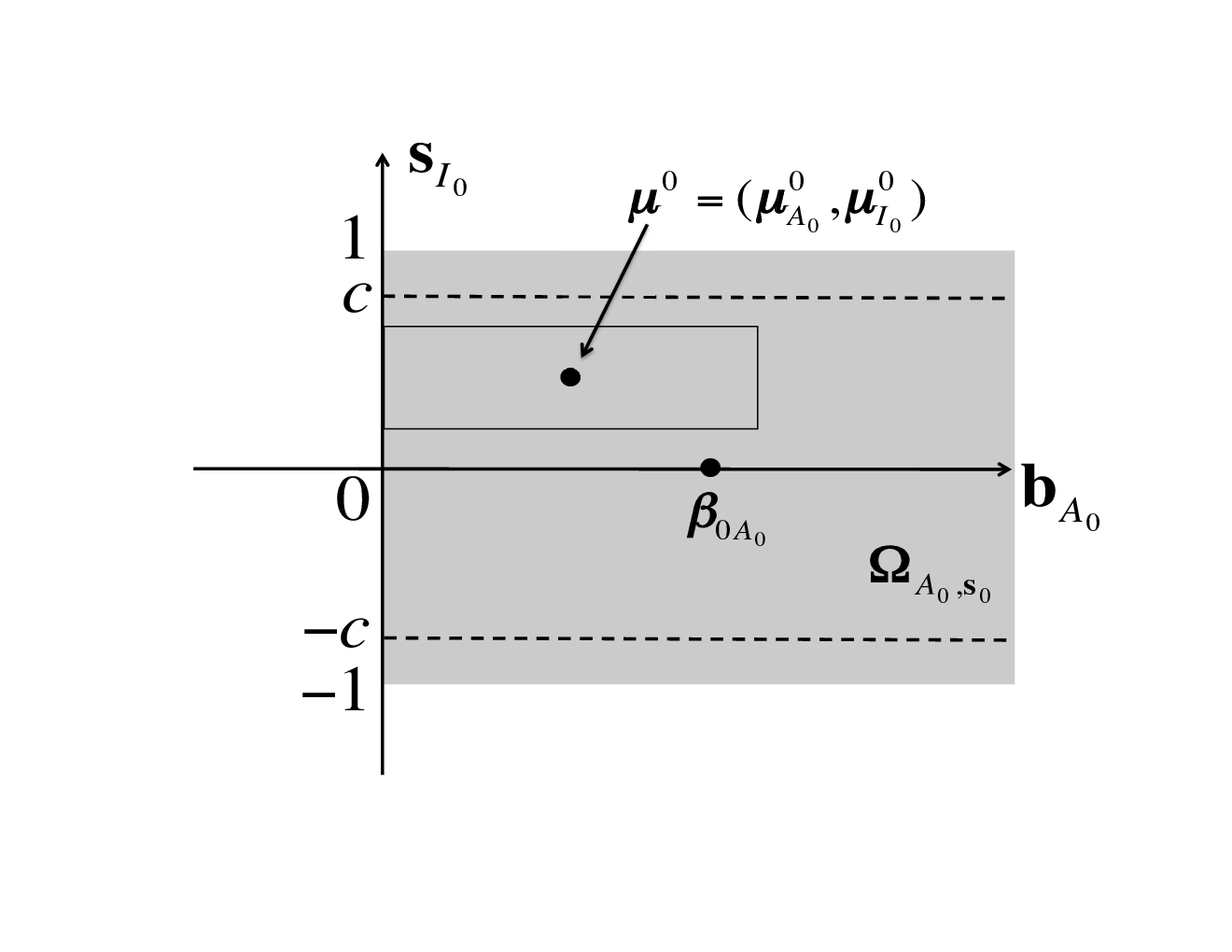
Let 𝐇A​(𝐛A,𝐬I,𝜷)=𝐇⁡(𝐛A,𝐬I,A,𝜷)\mathbf{H}_{A}(\mathbf{b}_{A},\mathbf{s}_{I};\bm{\beta})=\mathbf{H}(\mathbf{b}_{A},\mathbf{s}_{I},A;\bm{\beta}) for (𝐛A,𝐬I)∈ΩA(\mathbf{b}_{A},\mathbf{s}_{I})\in\Omega_{A} and UA=𝐇A​(ΩA,𝜷)U_{A}=\mathbf{H}_{A}(\Omega_{A};\bm{\beta}) be the image of ΩA\Omega_{A} under the map 𝐇A\mathbf{H}_{A}. Now imagine we plug different 𝐔∈ℝp\mathbf{U}\in\mathbb{R}^{p} into Equation (2.2) and solve for (𝜷^𝒜,𝐒ℐ,𝒜)(\hat{\bm{\beta}}_{\mathcal{A}},\mathbf{S}_{\mathcal{I}},\mathcal{A}). Then the set ΩA×{A}\Omega_{A}\times\{A\} is the collection of all possible solutions such that supp​(𝜷^)=A\text{supp}(\hat{\bm{\beta}})=A, the set UAU_{A} is the collection of all 𝐔\mathbf{U} that give these solutions, and 𝐇A\mathbf{H}_{A} is a bijection between the two sets. It is easy to see that Ω=⋃AΩA×{A}\Omega=\bigcup_{A}\Omega_{A}\times\{A\}, i.e., {ΩA×{A}}\{\Omega_{A}\times\{A\}\}, for AA extending over all subsets of {1,…,p}\{1,\ldots,p\}, form a partition of the space Ω\Omega. The bijective nature of 𝐇\mathbf{H} implies that {UA}\{U_{A}\} also form a partition of ℝp\mathbb{R}^{p}, the space of 𝐔\mathbf{U}. Figure 2 illustrates the bijection 𝐇\mathbf{H} for p=2p=2 and the space partitioning by AA. In this case, 𝐇A\mathbf{H}_{A} map the four subspaces ΩA\Omega_{A} for A=∅,{1},{2},{1,2}A=\varnothing,\{1\},\{2\},\{1,2\}, each in a different ℝ2\mathbb{R}^{2}, onto the space of 𝐔\mathbf{U} which is another ℝ2\mathbb{R}^{2}.

Refer to caption
Figure 2: The bijection 𝐇\mathbf{H}, its restrictions 𝐇A\mathbf{H}_{A}, the four subspaces ΩA\Omega_{A} (shaded areas) and the corresponding partition in the space of 𝐔\mathbf{U} for p=2p=2.
Remark 1.

The simple fact that 𝐇\mathbf{H} maps every point in Ω\Omega into row​(𝐗)=ℝp\text{row}(\mathbf{X})=\mathbb{R}^{p} is crucial to the derivation of the sampling distribution of (𝜷^𝒜,𝐒ℐ,𝒜)(\hat{\bm{\beta}}_{\mathcal{A}},\mathbf{S}_{\mathcal{I}},\mathcal{A}) in the low-dimensional setting. This means that every (𝐛A,𝐬I,A)∈Ω(\mathbf{b}_{A},\mathbf{s}_{I},A)\in\Omega is the solution to Equation (2.2) for 𝐔=𝐮=𝐇⁡(𝐛A,𝐬I,A,𝜷)\mathbf{U}=\mathbf{u}=\mathbf{H}(\mathbf{b}_{A},\mathbf{s}_{I},A;\bm{\beta}), and therefore one can simply find the probability density of (𝜷^𝒜,𝐒ℐ,𝒜)(\hat{\bm{\beta}}_{\mathcal{A}},\mathbf{S}_{\mathcal{I}},\mathcal{A}) at (𝐛A,𝐬I,A)(\mathbf{b}_{A},\mathbf{s}_{I},A) by the density of 𝐔\mathbf{U} at 𝐮\mathbf{u}. This is not the case when p>np>n (Section 4).

2.3 The sampling distribution

Now we can use the bijection 𝐇\mathbf{H} to find the distribution of (𝜷^𝒜,𝐒ℐ,𝒜)(\hat{\bm{\beta}}_{\mathcal{A}},\mathbf{S}_{\mathcal{I}},\mathcal{A}) from the distribution of 𝐔\mathbf{U}. Let ξk\xi_{k} denote kk-dimensional Lebesgue measure.

Theorem 1.

Assume that rank​(𝐗)=p\text{rank}(\mathbf{X})=p and let f𝐔f_{\mathbf{U}} be the probability density of 𝐔\mathbf{U} with respect to ξp\xi_{p}. For (𝐛A,𝐬I,A)∈Ω(\mathbf{b}_{A},\mathbf{s}_{I},A)\in\Omega, the joint distribution of (𝜷^𝒜,𝐒ℐ,𝒜)(\hat{\bm{\beta}}_{\mathcal{A}},\mathbf{S}_{\mathcal{I}},\mathcal{A}) is given by

P⁡(𝜷^A∈d​𝐛A,𝐒I∈d​𝐬I,𝒜=A)\displaystyle P(\hat{\bm{\beta}}_{A}\in d\mathbf{b}_{A},\mathbf{S}_{I}\in d\mathbf{s}_{I},\mathcal{A}=A) =\displaystyle= f𝐔​(𝐇⁡(𝐛A,𝐬I,A,𝜷))​|det𝐃⁡(A)|​ξp​(d​𝐛A​d​𝐬I)\displaystyle f_{\mathbf{U}}(\mathbf{H}(\mathbf{b}_{A},\mathbf{s}_{I},A;\bm{\beta}))|\det\mathbf{D}(A)|\xi_{p}(d\mathbf{b}_{A}d\mathbf{s}_{I}) (2.15)
=Δ\displaystyle\mathop{=}\limits^{\Delta} π⁡(𝐛A,𝐬I,A)​ξp​(d​𝐛A​d​𝐬I),\displaystyle\pi(\mathbf{b}_{A},\mathbf{s}_{I},A)\xi_{p}(d\mathbf{b}_{A}d\mathbf{s}_{I}),

and the distribution of (𝜷^𝒜,𝒜)(\hat{\bm{\beta}}_{\mathcal{A}},\mathcal{A}) is a marginal distribution given by

P⁡(𝜷^A∈d​𝐛A,𝒜=A)=[∫[−1,1]p−|A|π⁡(𝐛A,𝐬I,A)​ξp−|A|​(d​𝐬I)]​ξ|A|​(d​𝐛A).\displaystyle P(\hat{\bm{\beta}}_{A}\in d\mathbf{b}_{A},\mathcal{A}=A)=\left[\int_{[-1,1]^{p-|A|}}\pi(\mathbf{b}_{A},\mathbf{s}_{I},A)\xi_{p-|A|}(d\mathbf{s}_{I})\right]\xi_{|A|}(d\mathbf{b}_{A}). (2.16)
Proof.

Let 𝐮=𝐇⁡(𝐛A,𝐬I,A,𝜷)=𝐇A​(𝐛A,𝐬I,𝜷)\mathbf{u}=\mathbf{H}(\mathbf{b}_{A},\mathbf{s}_{I},A;\bm{\beta})=\mathbf{H}_{A}(\mathbf{b}_{A},\mathbf{s}_{I};\bm{\beta}). From (2.2) and (2.14), one sees that for any fixed AA, bj≠0b_{j}\neq 0 for all j∈Aj\in A and 𝐇A\mathbf{H}_{A} is differentiable. Differentiating 𝐮\mathbf{u} with respect to (𝐛A,𝐬I)(\mathbf{b}_{A},\mathbf{s}_{I}),

d​𝐮=∂𝐇A∂(𝐛A,𝐬I)𝖳​(d​𝐛Ad​𝐬I)=𝐃⁡(A)​(d​𝐛Ad​𝐬I)d\mathbf{u}=\frac{\partial\mathbf{H}_{A}}{\partial(\mathbf{b}_{A},\mathbf{s}_{I})^{\mathsf{T}}}\left(\begin{array}[]{l}d\mathbf{b}_{A}\\ d\mathbf{s}_{I}\end{array}\right)=\mathbf{D}(A)\left(\begin{array}[]{l}d\mathbf{b}_{A}\\ d\mathbf{s}_{I}\end{array}\right)

and thus ξp​(d​𝐮)=|det𝐃⁡(A)|​ξp​(d​𝐛A​d​𝐬I)\xi_{p}(d\mathbf{u})=|\det\mathbf{D}(A)|\xi_{p}(d\mathbf{b}_{A}d\mathbf{s}_{I}). Since 𝐇\mathbf{H} and 𝐇A:ΩA→UA\mathbf{H}_{A}:\Omega_{A}\to U_{A} are bijections, a change of variable gives

P⁡(𝜷^A∈d​𝐛A,𝐒I∈d​𝐬I,𝒜=A)=P⁡(𝐔∈d​𝐮)\displaystyle P(\hat{\bm{\beta}}_{A}\in d\mathbf{b}_{A},\,\mathbf{S}_{I}\in d\mathbf{s}_{I},\mathcal{A}=A)=P(\mathbf{U}\in d\mathbf{u})
=f𝐔​(𝐇⁡(𝐛A,𝐬I,A,𝜷))​|det𝐃⁡(A)|​ξp​(d​𝐛A​d​𝐬I).\displaystyle\quad\quad=f_{\mathbf{U}}(\mathbf{H}(\mathbf{b}_{A},\mathbf{s}_{I},A;\bm{\beta}))|\det\mathbf{D}(A)|\xi_{p}(d\mathbf{b}_{A}d\mathbf{s}_{I}).

Integrating (2.15) over 𝐬I∈[−1,1]p−|A|\mathbf{s}_{I}\in[-1,1]^{p-|A|} gives (2.16). ∎

Remark 2.

Equation (2.15) gives the joint distribution of (𝜷^𝒜,𝐒ℐ,𝒜)(\hat{\bm{\beta}}_{\mathcal{A}},\mathbf{S}_{\mathcal{I}},\mathcal{A}) and effectively the joint distribution of (𝜷^,𝐒)(\hat{\bm{\beta}},\mathbf{S}). The density π⁡(𝐛A,𝐬I,A)\pi(\mathbf{b}_{A},\mathbf{s}_{I},A) is defined with respect to the product of ξp\xi_{p} and counting measure on 2{1,…,p}2^{\{1,\ldots,p\}}. Analogously, the sampling distribution of 𝜷^\hat{\bm{\beta}} is given by the distribution of (𝜷^𝒜,𝒜)(\hat{\bm{\beta}}_{\mathcal{A}},\mathcal{A}) in (2.16). To be rigorous, (2.15) is derived by assuming that (𝐛A,𝐬I)(\mathbf{b}_{A},\mathbf{s}_{I}) is an interior point of ΩA\Omega_{A}. Note that (𝐛A,𝐬I)∈ΩA(\mathbf{b}_{A},\mathbf{s}_{I})\in\Omega_{A} is not in the interior if and only if |sj|=1|s_{j}|=1 for some j∈Ij\in I, and thus the Lebesgue measure of the union of these points is zero. Therefore, it will cause no problem at all to use π\pi as the density for all points in Ω\Omega. The joint distribution of (𝜷^𝒜,𝐒ℐ,𝒜)(\hat{\bm{\beta}}_{\mathcal{A}},\mathbf{S}_{\mathcal{I}},\mathcal{A}) has at least two nice properties which make it much more tractable than the distribution of 𝜷^\hat{\bm{\beta}}. First, the density π\pi does not involve multidimensional integral and has a closed-form expression that can be calculated explicitly if f𝐔f_{\mathbf{U}} is given. Second, the continuous components (𝜷^𝒜,𝐒ℐ)(\hat{\bm{\beta}}_{\mathcal{A}},\mathbf{S}_{\mathcal{I}}) always have the same dimension (=p)(=p) for any value of 𝒜\mathcal{A}, while 𝜷^𝒜\hat{\bm{\beta}}_{\mathcal{A}} lives in ℝ|𝒜|\mathbb{R}^{|\mathcal{A}|} whose dimension changes with 𝒜\mathcal{A}. These two properties are critical to the development of MCMC to sample from π\pi. See Section 3.1 for more discussion. We explicitly include the dominating Lebesgue measure to clarify the dimension of a density.

Remark 3.

The distribution of 𝜷^=(β^1,…,β^p)\hat{\bm{\beta}}=(\hat{\beta}_{1},\ldots,\hat{\beta}_{p}) in (2.16) is essentially defined for each AA. In many problems, one may be interested in the marginal distribution of β^j\hat{\beta}_{j} such as for calculating p-values and constructing confidence intervals. To obtain such a marginal distribution, we need to sum over all possible active sets, which cannot be done analytically. Our strategy is to draw samples from the joint distribution of (𝜷^𝒜,𝐒ℐ,𝒜)(\hat{\bm{\beta}}_{\mathcal{A}},\mathbf{S}_{\mathcal{I}},\mathcal{A}) by a Monte Carlo method. Then from the Monte Carlo samples one can easily approximate any marginal distribution of interest, such as that of β^j\hat{\beta}_{j}. This is exactly our motivation for estimator augmentation, which is in spirit similar to the use of auxiliary variables in the MCMC literature.

To further help our understanding of the density π\pi, consider a few conditional and marginal distributions derived from the joint distribution (2.15). First, the sampling distribution of the active set 𝒜\mathcal{A} is given by

P⁡(𝒜=A)=∫ΩAπ⁡(𝐛A,𝐬I,A)​ξp​(d​𝐛A​d​𝐬I)​=ΔZA,P(\mathcal{A}=A)=\int_{\Omega_{A}}\pi(\mathbf{b}_{A},\mathbf{s}_{I},A)\xi_{p}(d\mathbf{b}_{A}d\mathbf{s}_{I})\mathop{=}\limits^{\Delta}Z_{A}, (2.17)

where ΩA\Omega_{A} is the subspace for (𝜷^A,𝐒I)(\hat{\bm{\beta}}_{A},\mathbf{S}_{I}) defined in (2.14). In other words, ZAZ_{A} is the probability of ΩA×{A}\Omega_{A}\times\{A\} with respect to the joint distribution π\pi. Second, the conditional density of (𝜷^A,𝐒I)(\hat{\bm{\beta}}_{A},\mathbf{S}_{I}) given 𝒜=A\mathcal{A}=A (with respect to ξp\xi_{p}) is

π⁡(𝐛A,𝐬I∣A)=1ZA​π​(𝐛A,𝐬I,A)∝f𝐔​(𝐇⁡(𝐛A,𝐬I,A,𝜷))\pi(\mathbf{b}_{A},\mathbf{s}_{I}\mid A)=\frac{1}{Z_{A}}\pi(\mathbf{b}_{A},\mathbf{s}_{I},A)\propto f_{\mathbf{U}}(\mathbf{H}(\mathbf{b}_{A},\mathbf{s}_{I},A;\bm{\beta})) (2.18)

for (𝐛A,𝐬I)∈ΩA⊂ℝp(\mathbf{b}_{A},\mathbf{s}_{I})\in\Omega_{A}\subset\mathbb{R}^{p}. Using p=2p=2 as an illustration, the joint density π\pi is defined over all four shaded areas in Figure 2, while a conditional density π(⋅∣A)\pi(\cdot\mid A) is defined on each one of them. To give a concrete probability calculation, for a2>a1>0a_{2}>a_{1}>0,

P⁡(β^1∈[a1,a2],β^2=0)\displaystyle P(\hat{\beta}_{1}\in[a_{1},a_{2}],\hat{\beta}_{2}=0) =\displaystyle= P⁡(β^1∈[a1,a2],𝒜={1})\displaystyle P(\hat{\beta}_{1}\in[a_{1},a_{2}],\mathcal{A}=\{1\})
=\displaystyle= ∫a1a2∫−11π⁡(b1,s2,{1})​d​s2​d​b1,\displaystyle\int_{a_{1}}^{a_{2}}\int_{-1}^{1}\pi(b_{1},s_{2},\{1\})ds_{2}db_{1},

which is an integral over the rectangle [a1,a2]×[−1,1][a_{1},a_{2}]\times[-1,1] in Ω{1}\Omega_{\{1\}} (Figure 2). Clearly, this probability can be approximated by Monte Carlo integration if we have enough samples from π\pi.

Remark 4.

We emphasize that the weights wjw_{j} and the tuning parameter λ\lambda are assumed to be fixed in Theorem 1. For the adaptive Lasso, one may choose wj=|β~j|−1w_{j}=|\tilde{\beta}_{j}|^{-1} based on an initial estimate β~j\tilde{\beta}_{j}. The distribution (2.15) is valid for the adaptive Lasso only if we ignore the randomness in β~j\tilde{\beta}_{j} and regard wjw_{j} as constants during the repeated sampling procedure.

2.4 Normal errors

Denote by 𝒩k​(𝝁,𝚺)\mathcal{N}_{k}(\bm{\mu},\bm{\Sigma}) the kk-variate normal distribution with mean 𝝁\bm{\mu} and covariance matrix 𝚺\bm{\Sigma}, and by ϕk​(𝐳,𝝁,𝚺)\phi_{k}(\mathbf{z};\bm{\mu},\bm{\Sigma}) its probability density function. If the error 𝜺∼𝒩n​(𝟎,σ2​𝐈n)\bm{\varepsilon}\sim\mathcal{N}_{n}(\mathbf{0},\sigma^{2}\mathbf{I}_{n}) and rank​(𝐗)=p\text{rank}(\mathbf{X})=p, then 𝐔∼𝒩p​(𝟎,σ2n​𝐂)\mathbf{U}\sim\mathcal{N}_{p}(\mathbf{0},\frac{\sigma^{2}}{n}\mathbf{C}). In this case, the joint density π\pi (2.15) has a closed-form expression. Recall that 𝐬A=sgn​(𝐛A)\mathbf{s}_{A}=\mbox{sgn}(\mathbf{b}_{A}) and define

𝝁⁡(A,𝐬A,𝜷)\displaystyle\bm{\mu}(A,\mathbf{s}_{A};\bm{\beta}) =\displaystyle= [𝐃⁡(A)]−1​(𝐂​𝜷−λ​𝐖A​𝐬A),\displaystyle[\mathbf{D}(A)]^{-1}\left(\mathbf{C}\bm{\beta}-\lambda\mathbf{W}_{A}\mathbf{s}_{A}\right), (2.19)
𝚺⁡(A,σ2)\displaystyle\bm{\Sigma}(A;\sigma^{2}) =\displaystyle= σ2n​[𝐃⁡(A)]−1​𝐂​[𝐃⁡(A)]−𝖳.\displaystyle\frac{\sigma^{2}}{n}[\mathbf{D}(A)]^{-1}\mathbf{C}[\mathbf{D}(A)]^{-\mathsf{T}}. (2.20)
Corollary 1.

If rank​(𝐗)=p\text{rank}(\mathbf{X})=p and 𝜺∼𝒩n​(𝟎,σ2​𝐈n)\bm{\varepsilon}\sim\mathcal{N}_{n}(\mathbf{0},\sigma^{2}\mathbf{I}_{n}), then the joint density of (𝜷^𝒜,𝐒ℐ,𝒜)(\hat{\bm{\beta}}_{\mathcal{A}},\mathbf{S}_{\mathcal{I}},\mathcal{A}) is

π⁡(𝐛A,𝐬I,A)=ϕp​(𝐳,𝝁⁡(A,𝐬A,𝜷),𝚺⁡(A,σ2))​𝟏​((𝐳,A)∈Ω),\pi(\mathbf{b}_{A},\mathbf{s}_{I},A)=\phi_{p}(\mathbf{z};\bm{\mu}(A,\mathbf{s}_{A};\bm{\beta}),\bm{\Sigma}(A;\sigma^{2}))\bm{1}((\mathbf{z},A)\in\Omega), (2.21)

where 𝐳=(𝐛A,𝐬I)∈ℝp\mathbf{z}=(\mathbf{b}_{A},\mathbf{s}_{I})\in\mathbb{R}^{p} and 𝟏​(⋅)\bm{1}(\cdot) is an indicator function.

Proof.

First note that

𝐇⁡(𝐛A,𝐬I,A,𝜷)=𝐃⁡(A)​[𝐳−𝝁⁡(A,𝐬A,𝜷)].\mathbf{H}(\mathbf{b}_{A},\mathbf{s}_{I},A;\bm{\beta})=\mathbf{D}(A)[\mathbf{z}-\bm{\mu}(A,\mathbf{s}_{A};\bm{\beta})]. (2.22)

Under the assumptions, 𝐔∼𝒩p​(𝟎,σ2n​𝐂)\mathbf{U}\sim\mathcal{N}_{p}(\mathbf{0},\frac{\sigma^{2}}{n}\mathbf{C}). By Theorem 1,

π⁡(𝐛A,𝐬I,A)\displaystyle\pi(\mathbf{b}_{A},\mathbf{s}_{I},A) =\displaystyle= ϕp​(𝐃⁡(A)​[𝐳−𝝁⁡(A,𝐬A,𝜷)],𝟎,n−1​σ2​𝐂)​|det𝐃⁡(A)|\displaystyle\phi_{p}\left(\mathbf{D}(A)[\mathbf{z}-\bm{\mu}(A,\mathbf{s}_{A};\bm{\beta})];\mathbf{0},n^{-1}{\sigma^{2}}\mathbf{C}\right)|\det\mathbf{D}(A)|
=\displaystyle= ϕp​(𝐳,𝝁⁡(A,𝐬A,𝜷),n−1​σ2​[𝐃⁡(A)]−1​𝐂​[𝐃⁡(A)]−𝖳)\displaystyle\phi_{p}\left(\mathbf{z};\bm{\mu}(A,\mathbf{s}_{A};\bm{\beta}),n^{-1}{\sigma^{2}}[\mathbf{D}(A)]^{-1}\mathbf{C}[\mathbf{D}(A)]^{-\mathsf{T}}\right)
=\displaystyle= ϕp​(𝐳,𝝁⁡(A,𝐬A,𝜷),𝚺⁡(A,σ2))\displaystyle\phi_{p}(\mathbf{z};\bm{\mu}(A,\mathbf{s}_{A};\bm{\beta}),\bm{\Sigma}(A;\sigma^{2}))

for (𝐛A,𝐬I,A)=(𝐳,A)∈Ω(\mathbf{b}_{A},\mathbf{s}_{I},A)=(\mathbf{z},A)\in\Omega. ∎

Without the normal error assumption, Corollary 1 is still a good approximation when nn is large and pp is fixed, since n𝐔→d𝒩p(𝟎,σ2𝐂)\sqrt{n}\mathbf{U}\mathop{\to}\limits^{d}\mathcal{N}_{p}(\mathbf{0},\sigma^{2}\mathbf{C}) assuming 1n​𝐗𝖳​𝐗→𝐂>0\frac{1}{n}\mathbf{X}^{\mathsf{T}}\mathbf{X}\to\mathbf{C}>0 as n→∞n\to\infty.

Note that both the continuous components 𝐳\mathbf{z} and the active set AA are arguments of the density (2.21). For different AA and 𝐬A\mathbf{s}_{A}, the normal density ϕp\phi_{p} has different parameters. Given a particular A∗A^{*} and 𝐬∗∈{±1}|A∗|\mathbf{s}^{*}\in\{\pm 1\}^{|A^{*}|}, let I∗={1,…,p}∖A∗I^{*}=\{1,\ldots,p\}\setminus A^{*} and

ΩA∗,𝐬∗={(𝐛A∗,𝐬I∗)∈ΩA∗:sgn​(𝐛A∗)=𝐬∗}.\Omega_{A^{*},\mathbf{s}^{*}}=\{(\mathbf{b}_{A^{*}},\mathbf{s}_{I^{*}})\in\Omega_{A^{*}}:\mbox{sgn}(\mathbf{b}_{A^{*}})=\mathbf{s}^{*}\}. (2.23)

Then ΩA∗,𝐬∗×{A∗}\Omega_{A^{*},\mathbf{s}^{*}}\times\{A^{*}\} is the subset of Ω\Omega corresponding to the event {𝒜=A∗,sgn​(𝜷^A∗)=𝐬∗}\{\mathcal{A}=A^{*},\mbox{sgn}(\hat{\bm{\beta}}_{A^{*}})=\mathbf{s}^{*}\}. For 𝐳∈ΩA∗,𝐬∗\mathbf{z}\in\Omega_{A^{*},\mathbf{s}^{*}}, the density π⁡(𝐳,A∗)\pi(\mathbf{z},A^{*}) is identical to ϕp​(𝐳,𝝁⁡(A∗,𝐬∗,𝜷),𝚺⁡(A∗,σ2))\phi_{p}(\mathbf{z};\bm{\mu}(A^{*},\mathbf{s}^{*};\bm{\beta}),\bm{\Sigma}(A^{*};\sigma^{2})), i.e.,

π⁡(𝐳,A∗)​𝟏​(𝐳∈ΩA∗,𝐬∗)=ϕp​(𝐳,𝝁⁡(A∗,𝐬∗,𝜷),𝚺⁡(A∗,σ2))​𝟏​(𝐳∈ΩA∗,𝐬∗).\pi(\mathbf{z},A^{*})\bm{1}(\mathbf{z}\in\Omega_{A^{*},\mathbf{s}^{*}})=\phi_{p}(\mathbf{z};\bm{\mu}(A^{*},\mathbf{s}^{*};\bm{\beta}),\bm{\Sigma}(A^{*};\sigma^{2}))\bm{1}(\mathbf{z}\in\Omega_{A^{*},\mathbf{s}^{*}}).

Intuitively, this is because 𝐇\mathbf{H} restricted to A=A∗A=A^{*} and 𝐬A∗=𝐬∗\mathbf{s}_{A^{*}}=\mathbf{s}^{*} is simply an affine map [see (2.22)]. Consequently, the probability of ΩA∗,𝐬∗×{A∗}\Omega_{A^{*},\mathbf{s}^{*}}\times\{A^{*}\} with respect to π\pi is

P⁡(𝒜=A∗,sgn​(𝜷^A∗)=𝐬∗)=∫ΩA∗,𝐬∗ϕp​(𝐳,𝝁⁡(A∗,𝐬∗,𝜷),𝚺⁡(A∗,σ2))​ξp​(𝑑𝐳),P(\mathcal{A}=A^{*},\mbox{sgn}(\hat{\bm{\beta}}_{A^{*}})=\mathbf{s}^{*})=\int_{\Omega_{A^{*},\mathbf{s}^{*}}}\phi_{p}(\mathbf{z};\bm{\mu}(A^{*},\mathbf{s}^{*};\bm{\beta}),\bm{\Sigma}(A^{*};\sigma^{2}))\xi_{p}(d\mathbf{z}), (2.24)

and [𝜷^A∗,𝐒I∗∣𝒜=A∗,sgn(𝜷^A∗)=𝐬∗][\hat{\bm{\beta}}_{A^{*}},\mathbf{S}_{I^{*}}\mid\mathcal{A}=A^{*},\mbox{sgn}(\hat{\bm{\beta}}_{A^{*}})=\mathbf{s}^{*}] is the truncated 𝒩p​(𝝁⁡(A∗,𝐬∗,𝜷),𝚺⁡(A∗,σ2))\mathcal{N}_{p}(\bm{\mu}(A^{*},\mathbf{s}^{*};\bm{\beta}),\bm{\Sigma}(A^{*};\sigma^{2})) on ΩA∗,𝐬∗\Omega_{A^{*},\mathbf{s}^{*}}. For p=2p=2, if A∗={1}A^{*}=\{1\}, and 𝐬∗=−1\mathbf{s}^{*}=-1, the region Ω{1},−1=(−∞,0)×[−1,1]\Omega_{\{1\},-1}=(-\infty,0)\times[-1,1] is the left half of the Ω{1}\Omega_{\{1\}} in Figure 2 and the density π\pi restricted to this region is the same as the part of a bivariate normal density on the same region.

If 𝐂=𝐈p\mathbf{C}=\mathbf{I}_{p} and 𝐖=𝐈p\mathbf{W}=\mathbf{I}_{p}, the Lasso is equivalent to soft-thresholding the ordinary least-squares estimator 𝜷^OLS=(β^jOLS)1:p\hat{\bm{\beta}}^{\text{OLS}}=(\hat{\beta}^{\text{OLS}}_{j})_{1:p}. In this case, (2.19) and (2.20) have simpler forms:

𝝁⁡(A,𝐬A,𝜷)\displaystyle\bm{\mu}(A,\mathbf{s}_{A};\bm{\beta}) =\displaystyle= (𝜷A−λ​𝐬Aλ−1​𝜷I),\displaystyle\left(\begin{array}[]{c}\bm{\beta}_{A}-\lambda\mathbf{s}_{A}\\ \lambda^{-1}\bm{\beta}_{I}\end{array}\right),
𝚺⁡(A,σ2)\displaystyle\bm{\Sigma}(A;\sigma^{2}) =\displaystyle= σ2n​(𝐈|A|𝟎𝟎λ−2​𝐈|I|).\displaystyle\frac{\sigma^{2}}{n}\left(\begin{array}[]{cc}\mathbf{I}_{|A|}&\mathbf{0}\\ \mathbf{0}&\lambda^{-2}\mathbf{I}_{|I|}\end{array}\right).

By (2.24) we find, for example,

P⁡(𝒜=A,sgn​(𝜷^A)=(1,…,1))\displaystyle P(\mathcal{A}=A,\mbox{sgn}(\hat{\bm{\beta}}_{A})=(1,\ldots,1))
=∏j∈A∫0∞ϕ⁡(bj,βj−λ,σ2n)​d​bj⋅∏j∈I∫−11ϕ⁡(sj,βjλ,σ2λ2​n)​d​sj\displaystyle=\prod_{j\in A}\int_{0}^{\infty}\phi\left(b_{j};\beta_{j}-\lambda,\frac{\sigma^{2}}{n}\right)db_{j}\cdot\prod_{j\in I}\int_{-1}^{1}\phi\left(s_{j};\frac{\beta_{j}}{\lambda},\frac{\sigma^{2}}{\lambda^{2}n}\right)ds_{j}
=∏j∈AP⁡(β^jOLS>λ)⋅∏j∈IP⁡(|β^jOLS|≤λ),\displaystyle=\prod_{j\in A}P(\hat{\beta}^{\text{OLS}}_{j}>\lambda)\cdot\prod_{j\in I}P(|\hat{\beta}^{\text{OLS}}_{j}|\leq\lambda),

where the last equality is due to that 𝜷^OLS∼𝒩p​(𝜷,n−1​σ2​𝐈p)\hat{\bm{\beta}}^{\text{OLS}}\sim\mathcal{N}_{p}(\bm{\beta},n^{-1}\sigma^{2}\mathbf{I}_{p}). One sees that our result is consistent with that obtained directly from soft-thresholding each component of 𝜷^OLS\hat{\bm{\beta}}^{\text{OLS}} by λ\lambda.

2.5 Estimation

To apply Theorem 1 in practice, one needs to estimate f𝐔f_{\mathbf{U}} and 𝜷\bm{\beta} if they are not given. Suppose that f𝐔f_{\mathbf{U}} is estimated by f^𝐔\hat{f}_{\mathbf{U}} and 𝜷\bm{\beta} is estimated by 𝜷ˇ\check{\bm{\beta}}. Then, the corresponding estimate of the density π\pi is

π^​(𝐛A,𝐬I,A)=f^𝐔​(𝐇⁡(𝐛A,𝐬I,A,𝜷ˇ))​|det𝐃⁡(A)|.\hat{\pi}(\mathbf{b}_{A},\mathbf{s}_{I},A)=\hat{f}_{\mathbf{U}}(\mathbf{H}(\mathbf{b}_{A},\mathbf{s}_{I},A;\check{\bm{\beta}}))|\det\mathbf{D}(A)|. (2.27)

Since 𝔼⁡(𝐔)=𝟎\mathbb{E}(\mathbf{U})=\mathbf{0} and Var​(n​𝐔)=σ2​𝐂\text{Var}(\sqrt{n}\mathbf{U})=\sigma^{2}\mathbf{C}, estimating f𝐔f_{\mathbf{U}} reduces to estimating σ2\sigma^{2} when 𝜺\bm{\varepsilon} is normally distributed or when the sample size nn is large. A consistent estimator of σ2\sigma^{2} can be constructed given a consistent estimator of 𝜷\bm{\beta}. For example, when p<np<n one may use

σ^2=‖𝐲−𝐗​𝜷ˇ‖22n−p,\hat{\sigma}^{2}=\frac{\|\mathbf{y}-\mathbf{X}\check{\bm{\beta}}\|_{2}^{2}}{n-p}, (2.28)

provided that 𝜷ˇ\check{\bm{\beta}} is consistent for 𝜷\bm{\beta}. If 𝜺\bm{\varepsilon} does not follow a normal distribution, one can apply other parametric or nonparametric methods to estimate f𝐔f_{\mathbf{U}}. Here, we propose a bootstrap-based approach under the assumption that 𝐔\mathbf{U} is elliptically symmetric. That is, 𝐔~=𝐂−1/2𝐔\tilde{\mathbf{U}}=\mathbf{C}^{-1/2}\mathbf{U} is spherically symmetric: For 𝐯1,𝐯2∈ℝp\mathbf{v}_{1},\mathbf{v}_{2}\in\mathbb{R}^{p}, if ‖𝐯1‖2=‖𝐯2‖2\|\mathbf{v}_{1}\|_{2}=\|\mathbf{v}_{2}\|_{2} then f𝐔~​(𝐯1)=f𝐔~​(𝐯2)f_{\tilde{\mathbf{U}}}(\mathbf{v}_{1})=f_{\tilde{\mathbf{U}}}(\mathbf{v}_{2}), where f𝐔~f_{\tilde{\mathbf{U}}} is the density of 𝐔~\tilde{\mathbf{U}}. Generate bootstrap samples, 𝜺(i)=(ε1(i),…,εn(i))\bm{\varepsilon}^{(i)}=(\varepsilon^{(i)}_{1},\ldots,\varepsilon^{(i)}_{n}) for i=1,…,Ki=1,\ldots,K, by resampling with replacement from 𝜺^=(ε^1,…,ε^n)=𝐲−𝐗​𝜷ˇ\hat{\bm{\varepsilon}}=(\hat{\varepsilon}_{1},\ldots,\hat{\varepsilon}_{n})=\mathbf{y}-\mathbf{X}\check{\bm{\beta}}, and calculate 𝐔~(i)=1n𝐂−1/2𝐗𝖳𝜺(i)\tilde{\mathbf{U}}^{(i)}=\frac{1}{n}\mathbf{C}^{-1/2}\mathbf{X}^{\mathsf{T}}\bm{\varepsilon}^{(i)} for each ii. Given 0=h0<h1<⋯<hM<∞0=h_{0}<h_{1}<\cdots<h_{M}<\infty, let Km=|{i:hm−1≤‖𝐔~(i)‖2<hm}|K_{m}=|\{i:h_{m-1}\leq\|\tilde{\mathbf{U}}^{(i)}\|_{2}<h_{m}\}| for m=1,…,Mm=1,\ldots,M. The density of 𝐔~\tilde{\mathbf{U}} is then estimated by

f^𝐔~​(𝐯)∝∑m=1MKmhmp−hm−1p​𝟏​(hm−1≤‖𝐯‖2<hm)\hat{f}_{\tilde{\mathbf{U}}}(\mathbf{v})\propto\sum_{m=1}^{M}\frac{K_{m}}{h_{m}^{p}-h_{m-1}^{p}}\bm{1}(h_{m-1}\leq\|\mathbf{v}\|_{2}<h_{m}) (2.29)

for ‖𝐯‖2∈[0,hM)\|\mathbf{v}\|_{2}\in[0,h_{M}). The density for ‖𝐯‖2≥hM\|\mathbf{v}\|_{2}\geq h_{M} can be estimated by linear extrapolation of log⁡f^𝐔~\log\hat{f}_{\tilde{\mathbf{U}}}. Finally, set f^𝐔(𝐮)=f^𝐔~(𝐂−1/2𝐮)(det𝐂)−1/2\hat{f}_{\mathbf{U}}(\mathbf{u})=\hat{f}_{\tilde{\mathbf{U}}}(\mathbf{C}^{-1/2}\mathbf{u})(\det\mathbf{C})^{-1/2}.

In general, estimating f𝐔f_{\mathbf{U}} is difficult when pp is large. One may have to assume some parametric density for 𝐔\mathbf{U}, which reduces the problem to the estimation of a few unknown parameters. Besides normality, one may assume that 𝐔\mathbf{U} follows a multivariate tt distribution, which is motivated from a Bayesian perspective to be discussed in Section 7.3.

Sampling from π\pi or π^\hat{\pi} can be very useful for statistical inference based on a Lasso-type estimator. We may directly draw (𝜷∗,𝐒∗)({\bm{\beta}}^{*},\mathbf{S}^{*}) from π^\hat{\pi} given (𝜷ˇ,σ^)(\check{\bm{\beta}},\hat{\sigma}) and use the conditional distribution [(𝜷∗−𝜷ˇ)∣𝜷ˇ,σ^][({\bm{\beta}}^{*}-\check{\bm{\beta}})\mid\check{\bm{\beta}},\hat{\sigma}] to construct confidence regions around 𝜷^\hat{\bm{\beta}}. Under some assumptions, the conditional distribution [(𝜷∗−𝜷ˇ)∣𝜷ˇ,σ^][({\bm{\beta}}^{*}-\check{\bm{\beta}})\mid\check{\bm{\beta}},\hat{\sigma}] provides a valid approximation to the true sampling distribution of (𝜷^−𝜷)(\hat{\bm{\beta}}-\bm{\beta}). We derive nonasymptotic error bounds for this approximation in Section 6 after the development of our method in the high-dimensional setting. If 𝜷\bm{\beta} is specified in the null hypothesis in a significance test, then samples from π\pi can be used to calculate p-values. This aspect will be explored in Section 5.

3 MCMC algorithms

In this section, we develop MCMC algorithms to sample from π\pi given 𝜷\bm{\beta} and f𝐔f_{\mathbf{U}} (or σ2\sigma^{2}). Before that, we first introduce a direct sampling approach which includes the residual bootstrap method as a special case.

Routine 1 (Direct sampler).

Assume the error distribution is 𝒟⁡(𝟎,σ2​𝐈n)\mathcal{D}(\mathbf{0},\sigma^{2}\mathbf{I}_{n}). For t=1,…,Lt=1,\ldots,L

  • (1)

    draw 𝜺(t)∼𝒟⁡(𝟎,σ2​𝐈n)\bm{\varepsilon}^{(t)}\sim\mathcal{D}(\mathbf{0},\sigma^{2}\mathbf{I}_{n}) and set 𝐲(t)=𝐗​𝜷+𝜺(t)\mathbf{y}^{(t)}=\mathbf{X}\bm{\beta}+\bm{\varepsilon}^{(t)};

  • (2)

    find the minimizer 𝜷^(t)\hat{\bm{\beta}}^{(t)} of (1.2) with 𝐲(t)\mathbf{y}^{(t)} in place of 𝐲\mathbf{y};

  • (3)

    if needed, calculate the subgradient vector 𝐒(t)=(n​λ​𝐖)−1​𝐗𝖳​(𝐲(t)−𝐗​𝜷^(t))\mathbf{S}^{(t)}=(n\lambda\mathbf{W})^{-1}\mathbf{X}^{\mathsf{T}}(\mathbf{y}^{(t)}-\mathbf{X}\hat{\bm{\beta}}^{(t)}).

This approach directly draws 𝐲(t)\mathbf{y}^{(t)} from its sampling distribution and requires a numerical optimization algorithm in step (2) for each sample. Moreover, step (1) will be complicated if we cannot draw independent samples from 𝒟⁡(𝟎,σ2​𝐈n)\mathcal{D}(\mathbf{0},\sigma^{2}\mathbf{I}_{n}). If 𝜺(t)\bm{\varepsilon}^{(t)} is drawn by resampling residuals, then Routine 1 is equivalent to the bootstrap method of Knight and Fu (2000).

As the density π⁡(𝐛A,𝐬I,A){\pi}(\mathbf{b}_{A},\mathbf{s}_{I},A) (2.15) has a closed-form expression given 𝜷\bm{\beta} and f𝐔f_{\mathbf{U}}, MCMC and IS can be applied to sample from and calculate expectations with respect to the distribution. These methods may offer much more flexible and efficient alternatives to the direct sampling approach, although the samples are either dependent or weighted. In what follows, we propose a few special designs targeting at different applications to exemplify the use of MCMC methods. Examples of IS will be given in Section 5 under the high-dimensional setting.

3.1 Reversibility

Our goal is to design a reversible Markov chain on the space Ω\Omega, which is composed of a finite number of subspaces ΩA\Omega_{A}, each having the same dimension pp. Therefore, moves with an ordinary Metropolis-Hastings (MH) ratio are sufficient, which can be seen as follows. For any (𝐛A,𝐬I,A)∈Ω(\mathbf{b}_{A},\mathbf{s}_{I},A)\in\Omega, let 𝜽=(θ1,…,θp)\bm{\theta}=(\theta_{1},\ldots,\theta_{p}) with components given by

θj={bj if ​j∈Asj otherwise,\theta_{j}=\left\{\begin{array}[]{ll}b_{j}&\mbox{ if }j\in A\\ s_{j}&\mbox{ otherwise},\end{array}\right. (3.1)

i.e., 𝜽A=𝐛A\bm{\theta}_{A}=\mathbf{b}_{A} and 𝜽I=𝐬I\bm{\theta}_{I}=\mathbf{s}_{I}. Then our target distribution is π⁡(𝜽A,𝜽I,A)​ξp​(d​𝜽)\pi(\bm{\theta}_{A},\bm{\theta}_{I},A)\xi_{p}(d\bm{\theta}). Suppose that (𝜽,A)(\bm{\theta},A) is the current state and we have a proposal for a new state (𝜽†,A†)(\bm{\theta}^{{\dagger}},A^{{\dagger}}). In general, the proposal may only change some components of 𝜽\bm{\theta}, say θj\theta_{j} for j∈B⊆{1,…,p}j\in B\subseteq\{1,\ldots,p\}, such that 𝜽−B†=𝜽−B\bm{\theta}^{{\dagger}}_{-B}=\bm{\theta}_{-B}. Let q⁡((𝜽,A),(𝜽†,A†))q((\bm{\theta},A),(\bm{\theta}^{{\dagger}},A^{{\dagger}})) be the density of this proposal with respect to ξ|B|\xi_{|B|} and I†={1,…,p}∖A†I^{{\dagger}}=\{1,\ldots,p\}\setminus A^{{\dagger}}. The MH ratio in terms of probability measures is

min⁡{1,π⁡(𝜽A††,𝜽I††,A†)​ξp​(d​𝜽†)π⁡(𝜽A,𝜽I,A)​ξp​(d​𝜽)​q⁡((𝜽†,A†),(𝜽,A))​ξ|B|​(d​𝜽B)q⁡((𝜽,A),(𝜽†,A†))​ξ|B|​(d​𝜽B†)}\displaystyle\min\left\{1,\frac{\pi(\bm{\theta}^{{\dagger}}_{A^{{\dagger}}},\bm{\theta}^{{\dagger}}_{I^{{\dagger}}},A^{{\dagger}})\xi_{p}(d\bm{\theta}^{{\dagger}})}{\pi(\bm{\theta}_{A},\bm{\theta}_{I},A)\xi_{p}(d\bm{\theta})}\frac{q((\bm{\theta}^{{\dagger}},A^{{\dagger}}),(\bm{\theta},A))\xi_{|B|}(d\bm{\theta}_{B})}{q((\bm{\theta},A),(\bm{\theta}^{{\dagger}},A^{{\dagger}}))\xi_{|B|}(d\bm{\theta}^{{\dagger}}_{B})}\right\} (3.2)
=\displaystyle= min⁡{1,π⁡(𝜽A††,𝜽I††,A†)π⁡(𝜽A,𝜽I,A)​q⁡((𝜽†,A†),(𝜽,A))q⁡((𝜽,A),(𝜽†,A†))​ξp−|B|​(d​𝜽−B†)ξp−|B|​(d​𝜽−B)}.\displaystyle\min\left\{1,\frac{\pi(\bm{\theta}^{{\dagger}}_{A^{{\dagger}}},\bm{\theta}^{{\dagger}}_{I^{{\dagger}}},A^{{\dagger}})}{\pi(\bm{\theta}_{A},\bm{\theta}_{I},A)}\frac{q((\bm{\theta}^{{\dagger}},A^{{\dagger}}),(\bm{\theta},A))}{q((\bm{\theta},A),(\bm{\theta}^{{\dagger}},A^{{\dagger}}))}\frac{\xi_{p-|B|}(d\bm{\theta}^{{\dagger}}_{-B})}{\xi_{p-|B|}(d\bm{\theta}_{-B})}\right\}.

As 𝜽−B†=𝜽−B\bm{\theta}^{{\dagger}}_{-B}=\bm{\theta}_{-B}, the dominating measures in (3.2) cancel out and the ratio reduces to a standard MH ratio involving only densities.

Now we see that our strategy of estimator augmentation plays two roles in MCMC sampling. First, 𝐒ℐ\mathbf{S}_{\mathcal{I}} plays the role of an auxiliary variable: The target distribution π\pi for (𝜷^𝒜,𝐒ℐ,𝒜)(\hat{\bm{\beta}}_{\mathcal{A}},\mathbf{S}_{\mathcal{I}},\mathcal{A}) has a closed-form density which allows one to design an MCMC algorithm, while the distribution of interest, that for (𝜷^𝒜,𝒜)(\hat{\bm{\beta}}_{\mathcal{A}},\mathcal{A}), is a marginal distribution of π\pi without a closed-form density. Second, 𝐒ℐ\mathbf{S}_{\mathcal{I}} also plays the role of dimension matching so that the continuous components (𝜷^𝒜,𝐒ℐ)(\hat{\bm{\beta}}_{\mathcal{A}},\mathbf{S}_{\mathcal{I}}) always have the same dimension in any subspace. This eliminates the need for reversible jump MCMC (Green 1995). On the contrary, if we were to sample (𝜷^𝒜,𝒜)(\hat{\bm{\beta}}_{\mathcal{A}},\mathcal{A}) (assuming a closed-form approximation to its density), moves between two subspaces of different dimensions would require reversible jumps, which are usually much harder to design.

3.2 The MH Lasso sampler

We develop an MH algorithm, called the MH Lasso sampler (MLS), with coordinate-wise update. That is, to sequentially update each θj\theta_{j}, j=1,…,pj=1,\ldots,p, while holding other components fixed. Suppose the current state is (𝜽,A)(\bm{\theta},A). We design four moves to propose a new state (𝜽†,A†)(\bm{\theta}^{{\dagger}},A^{{\dagger}}), which are grouped into two types according to whether A†=AA^{{\dagger}}=A or not. In the following proposals, θj†=bj†\theta_{j}^{{\dagger}}=b_{j}^{{\dagger}} if j∈A†j\in A^{{\dagger}} and θj†=sj†\theta_{j}^{{\dagger}}=s_{j}^{{\dagger}} otherwise.

Definition 1.

Proposals in the MLS for a given j∈{1,…,p}j\in\{1,\ldots,p\}.

  • •

    Parameter-update proposals: (P1) If j∈Aj\in A, draw bj†∼𝒩⁡(bj,τj2)b_{j}^{{\dagger}}\sim\mathcal{N}(b_{j},\tau_{j}^{2}). (P2) If j∉Aj\notin A, draw sj†∼Unif​(−1,1)s_{j}^{{\dagger}}\sim\text{Unif}(-1,1). Set A†=AA^{{\dagger}}=A in both (P1) and (P2).

  • •

    Model-update proposals: (P3) If j∈Aj\in A, set A†=A∖{j}A^{{\dagger}}=A\setminus\{j\} and draw sj†∼Unif​(−1,1)s_{j}^{{\dagger}}\sim\text{Unif}(-1,1). (P4) If j∉Aj\notin A, set A†=A∪{j}A^{{\dagger}}=A\cup\{j\} and draw bj†∼𝒩⁡(0,τj2)b_{j}^{{\dagger}}\sim\mathcal{N}(0,\tau_{j}^{2}).

The two parameter-update proposals, (P1) and (P2), are symmetric. They only change the value of θj\theta_{j} and leave A†=AA^{{\dagger}}=A so that det𝐃⁡(A†)=det𝐃⁡(A)\det\mathbf{D}(A^{{\dagger}})=\det\mathbf{D}(A). From (2.15), one sees that the MH ratio is simply

min⁡{1,f𝐔​(𝐇⁡(𝜽A†,𝜽I†,A,𝜷))f𝐔​(𝐇⁡(𝜽A,𝜽I,A,𝜷))},\min\left\{1,\frac{f_{\mathbf{U}}(\mathbf{H}(\bm{\theta}^{{\dagger}}_{A},\bm{\theta}^{{\dagger}}_{I},A;\bm{\beta}))}{f_{\mathbf{U}}(\mathbf{H}(\bm{\theta}_{A},\bm{\theta}_{I},A;\bm{\beta}))}\right\},

which can be computed very efficiently, especially for a normal error distribution. The proposal (P3) removes a variable from the active set and (P4) adds a variable to the active set. Both propose moves between two subspaces. The two proposals are the reverse of each other and have a simple one-dimensional density. To be concrete, the MH ratio for proposal (P3) is

min⁡{1,π⁡(𝜽A††,𝜽I††,A†)π⁡(𝜽A,𝜽I,A)⋅ϕ⁡(bj,0,τj2)1/2},\min\left\{1,\frac{\pi(\bm{\theta}^{{\dagger}}_{A^{{\dagger}}},\bm{\theta}^{{\dagger}}_{I^{{\dagger}}},A^{{\dagger}})}{\pi(\bm{\theta}_{A},\bm{\theta}_{I},A)}\cdot\frac{\phi(b_{j};0,\tau^{2}_{j})}{1/2}\right\},

and analogously for proposal (P4). One needs to calculate the ratio between two determinants for these MH ratios,

|det𝐃⁡(A†)||det𝐃⁡(A)|=det𝐂A†​A†det𝐂A​A​(wj​λ)|A|−|A†|\frac{|\det\mathbf{D}(A^{\dagger})|}{|\det\mathbf{D}(A)|}=\frac{\det\mathbf{C}_{A^{{\dagger}}A^{{\dagger}}}}{\det\mathbf{C}_{AA}}(w_{j}\lambda)^{|A|-|A^{{\dagger}}|} (3.3)

by (2.13). As the two sets AA and A†A^{{\dagger}} differ by only one element, the ratio on the right-hand side can be calculated efficiently. When |A||A| is large, we use the sweep operator to dynamically update 𝐂A​A−1\mathbf{C}_{AA}^{-1} (the inverse of 𝐂A​A\mathbf{C}_{AA}) and obtain the ratio. See Appendix for further details. In general, however, a model-update proposal is more time-consuming than a parameter-update proposal.

This computational efficiency consideration motivates the following scheme in the MLS which uses both types of proposals. Let KK be an integer between 1 and pp and 𝜶=(αj)1:p\bm{\alpha}=(\alpha_{j})_{1:p} be a vector with every αj>0\alpha_{j}>0.

Routine 2 (MLS).

Suppose the current state is (𝜽(t),A(t))(\bm{\theta}^{(t)},A^{(t)}).

  • (1)

    Draw KK elements without replacement from {1,…,p}\{1,\ldots,p\} with the probability of drawing jj proportional to αj\alpha_{j} for each jj. Let M(t)M^{(t)} be the set of the KK elements.

  • (2)

    For j∈M(t)j\in M^{(t)}, sequentially update each θj\theta_{j} and the active set AA by an MH step with a model-update proposal.

  • (3)

    For j∉M(t)j\notin M^{(t)}, sequentially update each θj\theta_{j} by an MH step with a parameter-update proposal.

After the above pp MH steps in an iteration, the state is updated to (𝜽(t+1),A(t+1))(\bm{\theta}^{(t+1)},A^{(t+1)}).

The MLS has three input parameters, KK, 𝜶\bm{\alpha}, and (τj2)1:p(\tau^{2}_{j})_{1:p}. Specification of these parameters that gives good empirical performance will be provided in the numerical examples (Section 3.6).

3.3 The Gibbs Lasso sampler

Let aj=𝟏​(j∈A)a_{j}=\bm{1}(j\in A) and 𝐚=(aj)1:p\mathbf{a}=(a_{j})_{1:p}. Conditional densities π(θj,aj∣𝜽−j,𝐚−j)\pi(\theta_{j},a_{j}\mid\bm{\theta}_{-j},\mathbf{a}_{-j}) can be derived from the joint density π\pi, which allows for the development of a Gibbs sampler. However, as each conditional sampling step involves calculation of one-dimensional integrals and sampling from truncated distributions, the Gibbs sampler is more time-consuming and less efficient than the MLS for all examples on which we have tested these algorithms.

3.4 Conditioning on active set

Suppose that we have constructed a Lasso-type estimate 𝜷^∗\hat{\bm{\beta}}^{*} from an observed dataset and the set of selected variables is A∗A^{*}, which defines an estimated model. One may want to study the sampling distribution of the estimator given the estimated model, i.e., [𝜷^A∗∣𝒜=A∗][\hat{\bm{\beta}}_{A^{*}}\mid\mathcal{A}=A^{*}]. Confidence intervals of penalized estimators have been constructed by approximating this distribution via local expansion of the ℓ1\ell_{1} norm (Fan and Li 2001; Zou 2006). Since local approximation may not be accurate for a finite sample, Monte Carlo sampling from this conditional distribution may provide more accurate results. However, the direct sampling approach is not applicable in practice, because 𝒜=A∗\mathcal{A}=A^{*} is often a rare event unless pp is very small. On the contrary, it is very efficient to draw samples by an MH algorithm from the conditional distribution

π⁡(𝐛A∗,𝐬I∗∣A∗)∝f𝐔​(𝐇⁡(𝐛A∗,𝐬I∗,A∗,𝜷)),{\pi}(\mathbf{b}_{A^{*}},\mathbf{s}_{I^{*}}\mid A^{*})\propto{f}_{\mathbf{U}}(\mathbf{H}(\mathbf{b}_{A^{*}},\mathbf{s}_{I^{*}},A^{*};\bm{\beta})), (3.4)

where I∗={1,…,p}∖A∗I^{*}=\{1,\ldots,p\}\setminus A^{*}, according to (2.18). The distribution of interest, [𝜷^A∗∣𝒜=A∗][\hat{\bm{\beta}}_{A^{*}}\mid\mathcal{A}=A^{*}], is a marginal distribution of (3.4). Since evaluation of this density does not involve calculation of determinants, each MH step is very fast.

Routine 3 (MLS given active set).

Given the current state (𝐛A∗(t),𝐬I∗(t))(\mathbf{b}_{A^{*}}^{(t)},\mathbf{s}_{I^{*}}^{(t)}), sequentially draw bj(t+1)b_{j}^{(t+1)} for each j∈A∗j\in A^{*} by an MH step with proposal (P1) and sj(t+1)s_{j}^{(t+1)} for each j∉A∗j\notin A^{*} with proposal (P2) in one iteration.

3.5 Reparameterization view

To ease notation, write 𝜽=(𝜽A,𝜽I)\bm{\theta}=(\bm{\theta}_{A},\bm{\theta}_{I}) and 𝐇A​(𝜽)=𝐇⁡(𝜽,A)=𝐇⁡(𝜽A,𝜽I,A,𝜷)\mathbf{H}_{A}(\bm{\theta})=\mathbf{H}(\bm{\theta},A)=\mathbf{H}(\bm{\theta}_{A},\bm{\theta}_{I},A;\bm{\beta}) for 𝜽\bm{\theta} defined in (3.1). Suppose that (𝜽(t),A(t))(\bm{\theta}^{(t)},A^{(t)}) are simulated by the MLS (Routine 2) and let 𝐮(t)=𝐇⁡(𝜽(t),A(t))\mathbf{u}^{(t)}=\mathbf{H}(\bm{\theta}^{(t)},A^{(t)}). Since 𝐇\mathbf{H} is a bijection, 𝐮(t)\mathbf{u}^{(t)} is a Markov chain that leaves f𝐔f_{\mathbf{U}} invariant. Therefore, the MLS can be understood as an MH algorithm targeting at f𝐔f_{\mathbf{U}} with moves designed under local reparameterization, 𝜽=𝐇A−1​(𝐮)\bm{\theta}=\mathbf{H}_{A}^{-1}(\mathbf{u}) for 𝐮∈UA=𝐇A​(ΩA,𝜷)\mathbf{u}\in U_{A}=\mathbf{H}_{A}(\Omega_{A};\bm{\beta}) (2.14). The Jacobian of this reparameterization is [𝐃⁡(A)]−1[\mathbf{D}(A)]^{-1}. Under this view, the MH ratio for a proposal 𝐮†=𝐇⁡(𝜽†,A†)\mathbf{u}^{{\dagger}}=\mathbf{H}(\bm{\theta}^{{\dagger}},{A^{\dagger}}) given the current 𝐮\mathbf{u} is

min⁡{1,f𝐔​(𝐮†)f𝐔​(𝐮)​q⁡((𝜽†,A†),(𝜽,A))​|det𝐃⁡(A)|−1q⁡((𝜽,A),(𝜽†,A†))​|det𝐃⁡(A†)|−1},\min\left\{1,\frac{f_{\mathbf{U}}(\mathbf{u}^{{\dagger}})}{f_{\mathbf{U}}(\mathbf{u})}\frac{q((\bm{\theta}^{{\dagger}},A^{{\dagger}}),(\bm{\theta},A))|\det\mathbf{D}(A)|^{-1}}{q((\bm{\theta},A),(\bm{\theta}^{{\dagger}},A^{{\dagger}}))|\det\mathbf{D}(A^{\dagger})|^{-1}}\right\},

which of course coincides with (3.2). Moreover, when A=A†A=A^{{\dagger}} such as in proposals (P1) and (P2), the Jacobian determinants cancel out as we are using the same reparameterization 𝐇A−1\mathbf{H}_{A}^{-1} for both the proposal and the current state. Otherwise, the ratio of the Jacobian determinants accounts for the use of different reparameterizations. Clearly, if 𝐮(t)∼f𝐔\mathbf{u}^{(t)}\sim f_{\mathbf{U}} then (𝜽(t),A(t))∼π(\bm{\theta}^{(t)},A^{(t)})\sim\pi.

This view provides an insight into the computational efficiency of the MLS. Under normal error assumption, f𝐔f_{\mathbf{U}} is the density of a multivariate normal distribution, for which a simple MH algorithm is computationally tractable and can be quite efficient. We make a comparison with the direct sampler at a conceptual level. The direct sampler draws 𝐔\mathbf{U} via a linear transformation of 𝜺∼𝒩n​(𝟎,σ2​𝐈n)\bm{\varepsilon}\sim\mathcal{N}_{n}(\mathbf{0},\sigma^{2}\mathbf{I}_{n}), which costs nn draws from a univariate normal distribution followed by a multiplication with a size p×np\times n matrix. After that, we find (𝜽,A)=𝐇−1​(𝐔)(\bm{\theta},A)=\mathbf{H}^{-1}(\mathbf{U}) by numerical minimization due to the lack of a closed-form inverse of the mapping 𝐇\mathbf{H}. The MLS draws pp (<n<n) univariate proposals in one iteration, and does not need any numerical procedure to map 𝐮(t)\mathbf{u}^{(t)} back to the space Ω\Omega of (𝜽,A)(\bm{\theta},A) since the moves are by design in that space already. The mapping 𝐇\mathbf{H} from (𝜽(t),A(t))(\bm{\theta}^{(t)},A^{(t)}) to 𝐮(t)\mathbf{u}^{(t)} is simple and can be calculated analytically. This is fundamentally different from direct sampling which replies on a numerical procedure to find the image of each draw of 𝐔\mathbf{U} under the mapping 𝐇−1\mathbf{H}^{-1}. The relatively time-consuming step in the MLS is calculating the ratio (3.3) when a model-update proposal is used, which can be done by at most sweeping a |A|×|A||A|\times|A| matrix on a single position (Appendix). Owing to sparsity, |A||A| is usually much smaller than pp, which greatly speeds up this step. Since the target distribution in the space of 𝐔\mathbf{U} has a nice unimodal density, the chain 𝐮(t)\mathbf{u}^{(t)} often converges fast and has low autocorrelation. Consequently, we expect to see efficiency gain over direct sampling for the same amount of computing time, which will be confirmed numerically in the next subsection.

As in the following routine, by a special initialization such that (𝜽(1),A(1))∼π(\bm{\theta}^{(1)},A^{(1)})\sim\pi, the MLS can reach equilibrium in one step, which totally removes the need for burn-in iterations. This will make our method suitable for parallel computing. See Section 7.4 for a more detailed discussion. However, to demonstrate the efficiency of the MLS as an independent method, we did not use Routine 4 in the numerical results.

Routine 4.

Draw (𝐛(1),𝐬(1))(\mathbf{b}^{(1)},\mathbf{s}^{(1)}) from the direct sampler and let (𝜽(1),A(1))(\bm{\theta}^{(1)},A^{(1)}) be its equivalent representation. With (𝜽(1),A(1))(\bm{\theta}^{(1)},A^{(1)}) as the initial state, generate (𝜽(t),A(t))(\bm{\theta}^{(t)},A^{(t)}) for t=2,…,Nt=2,\ldots,N by an MCMC algorithm targeting at π\pi.

3.6 Numerical examples

We demonstrate with numerical examples the effectiveness of the above MCMC algorithms by comparing against the direct sampling approach. To this end, we simulated four datasets with different combinations of nn, pp, and σ2\sigma^{2} (Table 1). The vector of true coefficients 𝜷0\bm{\beta}_{0} has 10 nonzero components, β0​j=1\beta_{0j}=1 for j=1,…,5j=1,\ldots,5 and β0​j=−1\beta_{0j}=-1 for j=6,…,10j=6,\ldots,10. Each row of 𝐗\mathbf{X} was generated independently from 𝒩p​(𝟎,𝚺𝐗)\mathcal{N}_{p}(\mathbf{0},\bm{\Sigma}_{\mathbf{X}}), where the diagonal and the off-diagonal elements of 𝚺𝐗\bm{\Sigma}_{\mathbf{X}} are 1 and 0.250.25, respectively. Given the design matrix 𝐗\mathbf{X}, the response vector 𝐲\mathbf{y} was drawn from 𝒩n​(𝐗​𝜷0,σ2​𝐈n)\mathcal{N}_{n}(\mathbf{X}\bm{\beta}_{0},\sigma^{2}\mathbf{I}_{n}).

Table 1: Simulated datasets for MCMC
Dataset A B C D
(n,p,σ2)(n,p,\sigma^{2}) (500,100,1)(500,100,1) (500,200,1)(500,200,1) (300,100,4)(300,100,4) (300,200,4)(300,200,4)
|A∗||A^{*}| 23 22 25 57

The weights wjw_{j} (1.2) were set to 1 for all the following numerical results. The Lars package by Hastie and Efron was applied to find the solution path for each dataset. The value of λ\lambda was chosen by minimizing the CpC_{p} criterion implemented in the package, which determined the estimated coefficients, 𝜷^∗=(β^1∗,…,β^p∗)\hat{\bm{\beta}}^{*}=(\hat{\beta}^{*}_{1},\ldots,\hat{\beta}^{*}_{p}), of a dataset. The number of selected variables, |A∗||A^{*}|, for each dataset is given in Table 1. We considered two types of error distributions, the normal distribution and the elliptically symmetric distribution. Correspondingly, we calculated σ^2\hat{\sigma}^{2} by (2.28) with 𝜷ˇ=𝜷^∗\check{\bm{\beta}}=\hat{\bm{\beta}}^{*} or constructed f^𝐔\hat{f}_{\mathbf{U}} by the approach in Section 2.5. For all the results, step (2) of the direct sampler (Routine 1) was implemented with the Lars package.

We first examined the performance of the MLS on sampling from the joint distribution (2.15) given 𝜷^∗\hat{\bm{\beta}}^{*} and σ^2\hat{\sigma}^{2} or f^𝐔\hat{f}_{\mathbf{U}}. Let ωj=Φ(−|β^j∗|/ζj)\omega_{j}=\Phi(-|\hat{\beta}^{*}_{j}|/\zeta_{j}) for j=1,…,pj=1,\ldots,p, where ζj\zeta_{j} is the standard error of β^jOLS\hat{\beta}^{\text{OLS}}_{j} and Φ\Phi is the cumulative distribution function of 𝒩⁡(0,1)\mathcal{N}(0,1). We set K=p/5K=p/5 and αj∝ωj+ω0\alpha_{j}\propto\omega_{j}+\omega_{0}, where ω0=∑jωj/(5​p)\omega_{0}=\sum_{j}\omega_{j}/(5p) serves as a baseline weight so that each variable has a reasonable chance to be selected for model-update proposals. See Routine 2 for notations. Under this setting, if the estimate β^j∗\hat{\beta}^{*}_{j} is close to zero relative to ζj\zeta_{j}, it will have a higher chance for model-update proposals. The τj\tau_{j} used in the proposals (Definition 1) was set to 2​ζj2\zeta_{j}. The MLS was applied to each dataset 10 times independently. Each run consisted of L=5,500L=5,500 iterations with the first 500 as the burn-in period. In what follows, the sampler is abbreviated as MLSn and MLSe under the normal and the elliptically symmetric error distributions, respectively.

Figure 1(a) is the scatter plot of the samples of β^1\hat{\beta}_{1} and β^50\hat{\beta}_{50}, and illustrates that the distributions of some β^j\hat{\beta}_{j} indeed have a point mass at zero. The histogram of the subgradient S50S_{50} is shown in Figure 1(b) with two point masses on ±1\pm 1 and otherwise continuous. Mixing of the MLS was fast, as demonstrated with two chains in Figure 1(c), where the initial values were chosen to be about 20 standard deviations away from each other. Figure 1(d) shows the fast decay of the autocorrelation among the samples of a β^j\hat{\beta}_{j}, decreasing to below 0.05 in 10 to 15 iterations. The acceptance rate of the model-update proposals was generally between 0.2 and 0.4. For the parameter-update proposals, the acceptance rate was between 0.2 and 0.4 for (P1) and was higher than 0.6 for (P2), which is an independent proposal.

From the MCMC samples, we estimated the selection probability Ps,j=P⁡(β^j≠0)P_{s,j}=P(\hat{\beta}_{j}\neq 0), the 2.5% and the 97.5% quantiles of β^j\hat{\beta}_{j}, and the mean and the standard deviation of the conditional distribution [β^j∣β^j≠0][\hat{\beta}_{j}\mid\hat{\beta}_{j}\neq 0] for each jj. Since theoretical values are not available, we applied the direct sampling approach to simulate 5,000 independent samples for each dataset under the normal error distribution. These independent samples were used to estimate the above quantities as the ground truth. The MSEs across 10 independent runs of the MLS were calculated, and reported in Table 2 are the average MSEs over all jj for estimating the above five quantities. One clearly sees that all the estimates were very accurate. The MSE of the MLSe was greater than, but on the same order as, that of the MLSn for most estimates, which is expected due to the loss of efficiency without assuming a normal error distribution.

Table 2: MSE comparison for simulation from the joint sampling distribution
Method PsP_{s} 2.5% 97.5% mean SD
MLSn 3.38×10−43.38\times 10^{-4} 1.82×10−51.82\times 10^{-5} 1.79×10−51.79\times 10^{-5} 4.36×10−64.36\times 10^{-6} 2.78×10−62.78\times 10^{-6}
A MLSe 1.29 1.20 1.19 0.97 1.38
DSn 1.11 2.28 2.45 2.23 2.53
MLSn 2.13×10−42.13\times 10^{-4} 2.89×10−52.89\times 10^{-5} 1.74×10−51.74\times 10^{-5} 1.22×10−51.22\times 10^{-5} 8.44×10−68.44\times 10^{-6}
B MLSe 1.20 1.07 1.10 1.08 1.30
DSn 1.26 1.97 1.89 2.29 2.74
MLSn 4.14×10−44.14\times 10^{-4} 1.23×10−41.23\times 10^{-4} 1.24×10−41.24\times 10^{-4} 3.20×10−53.20\times 10^{-5} 2.28×10−52.28\times 10^{-5}
C MLSe 1.55 2.09 1.78 1.03 2.46
DSn 0.47 1.18 1.33 1.24 1.39
MLSn 4.34×10−44.34\times 10^{-4} 2.96×10−42.96\times 10^{-4} 2.85×10−42.85\times 10^{-4} 6.37×10−56.37\times 10^{-5} 5.02×10−55.02\times 10^{-5}
D MLSe 2.74 3.81 3.61 1.17 5.70
DSn 0.69 1.52 1.34 1.21 1.57

Note: For the MLSe and the DSn, reported is the ratio of MSE to that of the MLSn. The sweep operator was used in the MLS to calculate determinant ratios for dataset D.

We compared the efficiency of the MLS against the direct sampler (DSn) under the same amount of running time and under the same normal error distribution. The DSn generated around 500 samples in the same amount of time for 5,500 iterations of the MLSn. The ratio of the MSE of the DSn to that of the MLSn was calculated for each estimate (Table 2). For most estimates, the MLSn seems to be more efficient and may reduce the MSE by 10% to 60%. The improvement was more significant for datasets A and B where the sample size n=500n=500. For the other two datasets, the MLSn showed a higher MSE in estimating selection probabilities but was more accurate for all other estimates. Furthermore, if the error distribution is more complicated such that one cannot simulate samples independently from the distribution, the efficiency of the direct sampler may be even lower. These results clearly confirm the notion that the MLS can serve as an efficient alternative to the direct sampling method for simulating from the sampling distribution of a Lasso-type estimator.

Next, we implemented Routine 3 to sample from the conditional distribution of 𝜷^\hat{\bm{\beta}} given the model selected according to the CpC_{p} criterion, i.e., [𝜷^A∗∣𝒜=A∗][\hat{\bm{\beta}}_{A^{*}}\mid\mathcal{A}=A^{*}] with |A∗||A^{*}| given in Table 1. The same parameter setting as that in the previous example was used to run the MLSn and the MLSe. We estimated the 2.5% and the 97.5% quantiles, the mean, and the standard deviation of β^j\hat{\beta}_{j} for j∈A∗j\in A^{*}. The model space is composed of 2p2^{p} models, and the probability of the model A∗A^{*}, P⁡(𝒜=A∗)P(\mathcal{A}=A^{*}), is practically zero for the datasets used here. Therefore, the direct sampling approach is not applicable. This shows the advantage and flexibility of the Monte Carlo algorithms. Since we cannot construct ground truth for this example, the accuracy of an estimate is measured by its variance across 10 independent runs of the MLS, averaging over j∈A∗j\in A^{*} (Table 3). The variance of every estimate was on the order of 10−510^{-5} or smaller for datasets A, B and C and was on the order of 10−410^{-4} or smaller for dataset D under both error models. This highlights the stability of the MLS in approximating sampling distributions across different runs. There were cases in which the variance of the MLSe was smaller. This does not necessarily suggest that the MLSe provided a more accurate estimate, as the loss of efficiency without the normal error assumption is likely to result in a higher bias.

Table 3: Variance comparison for conditional sampling given active set
Method 2.5% 97.5% mean SD
A MLSn 1.21×10−51.21\times 10^{-5} 1.28×10−51.28\times 10^{-5} 2.21×10−62.21\times 10^{-6} 1.03×10−61.03\times 10^{-6}
MLSe 0.90 1.02 0.92 1.05
B MLSn 1.47×10−51.47\times 10^{-5} 1.19×10−51.19\times 10^{-5} 3.19×10−63.19\times 10^{-6} 9.60×10−79.60\times 10^{-7}
MLSe 1.22 1.15 1.02 1.23
C MLSn 7.66×10−57.66\times 10^{-5} 8.65×10−58.65\times 10^{-5} 1.59×10−51.59\times 10^{-5} 7.08×10−67.08\times 10^{-6}
MLSe 1.07 0.95 1.01 1.00
D MLSn 1.67×10−41.67\times 10^{-4} 1.78×10−41.78\times 10^{-4} 2.55×10−52.55\times 10^{-5} 1.28×10−51.28\times 10^{-5}
MLSe 0.77 0.97 0.77 0.79

Note: Variance of the MLSe is reported as the ratio to that of the MLSn.

4 High-dimensional setting

Recent efforts have established theoretical properties of ℓ1\ell_{1}-penalized linear regression in high dimension with p>np>n (Meinshausen and Bühlmann 2006; Zhao and Yu 2006; Zhang and Huang 2008; Bickel et al. 2009). Under this setting, we assume rank​(𝐗)=n<p\text{rank}(\mathbf{X})=n<p. Consequently, row​(𝐗)\text{row}(\mathbf{X}) is an nn-dimensional subspace of ℝp\mathbb{R}^{p} and the Gram matrix 𝐂\mathbf{C} has nn positive eigenvalues, denoted by Λj>0\Lambda_{j}>0, j=1,…,nj=1,\ldots,n. The associated orthonormal eigenvectors 𝐯j∈ℝp\mathbf{v}_{j}\in\mathbb{R}^{p}, j=1,…,nj=1,\ldots,n, form a basis for row​(𝐗)\text{row}(\mathbf{X}). Choose orthonormal vectors 𝐯p+1,…,𝐯p\mathbf{v}_{p+1},\ldots,\mathbf{v}_{p} to form a basis for the null space of 𝐗\mathbf{X}, null​(𝐗)\text{null}(\mathbf{X}), and let 𝐕=(𝐯1​|…|​𝐯p)\mathbf{V}=(\mathbf{v}_{1}|\ldots|\mathbf{v}_{p}). Then R={1,…,n}R=\{1,\ldots,n\} and N={n+1,…,p}N=\{n+1,\ldots,p\} index the columns of 𝐕\mathbf{V} that form respective bases for row​(𝐗)\text{row}(\mathbf{X}) and null​(𝐗)\text{null}(\mathbf{X}).

Assumption 1.

Every nn columns of 𝐗\mathbf{X} are linearly independent and every (p−n)(p-n) rows of 𝐕N\mathbf{V}_{N} are linearly independent.

The first part of this assumption is sufficient for the columns of 𝐗\mathbf{X} being in general position, which guarantees that (𝜷^,𝐒)(\hat{\bm{\beta}},\mathbf{S}) is unique for any 𝐲\mathbf{y} and λ>0\lambda>0 (Lemma 1). The second part will ease our derivation of the joint density of the augmented estimator. Note that Assumption 1 holds with probability one if the entries of 𝐗\mathbf{X} are drawn from a continuous distribution on ℝn×p\mathbb{R}^{n\times p}.

4.1 The bijection

Although 𝐔=1n​𝐗𝖳​𝜺\mathbf{U}=\frac{1}{n}\mathbf{X}^{\mathsf{T}}\bm{\varepsilon} is a pp-vector, by definition it always lies in row​(𝐗)\text{row}(\mathbf{X}). Therefore, 𝐕N𝖳​𝐔=𝟎\mathbf{V}_{N}^{\mathsf{T}}\mathbf{U}=\mathbf{0} and the nn-vector 𝐑=𝐕R𝖳​𝐔\mathbf{R}=\mathbf{V}_{R}^{\mathsf{T}}\mathbf{U} gives the coordinates of 𝐔\mathbf{U} with respect to the basis 𝐕R\mathbf{V}_{R}. If 𝜺\bm{\varepsilon} follows a continuous distribution on ℝn\mathbb{R}^{n}, then 𝐑\mathbf{R} has a proper density with respect to ξn\xi_{n}. For example, if 𝜺∼𝒩n​(𝟎,σ2​𝐈n)\bm{\varepsilon}\sim\mathcal{N}_{n}(\mathbf{0},\sigma^{2}\mathbf{I}_{n}), then 𝐑∼𝒩n​(𝟎,σ2n​𝚲)\mathbf{R}\sim\mathcal{N}_{n}(\mathbf{0},\frac{\sigma^{2}}{n}\bm{\Lambda}) with 𝚲=diag​(Λ1,…,Λn)\bm{\Lambda}=\mbox{diag}(\Lambda_{1},\ldots,\Lambda_{n}). Now 𝐑\mathbf{R} plays the same role as 𝐔\mathbf{U} does in the low-dimensional case. We will use the known distribution of 𝐑\mathbf{R} to derive the distribution of the augmented estimator (𝜷^𝒜,𝐒ℐ,𝒜)(\hat{\bm{\beta}}_{\mathcal{A}},\mathbf{S}_{\mathcal{I}},\mathcal{A}).

However, a technical difficulty is that when p>np>n, the map 𝐇\mathbf{H} defined in (2.2) is not a mapping from Ω\Omega to row​(𝐗)\text{row}(\mathbf{X}) as 𝐇⁡(𝐛A,𝐬I,A,𝜷)∈ℝp\mathbf{H}(\mathbf{b}_{A},\mathbf{s}_{I},A;\bm{\beta})\in\mathbb{R}^{p} is not necessarily in row​(𝐗)\text{row}(\mathbf{X}) for every (𝐛A,𝐬I,A)∈Ω(\mathbf{b}_{A},\mathbf{s}_{I},A)\in\Omega. We thus need to remove those “illegal” points in Ω\Omega so that the image of 𝐇\mathbf{H} always lies in the row space of 𝐗\mathbf{X}. This is achieved by imposing the constraint that

𝐕N𝖳​𝐇​(𝜷^𝒜,𝐒ℐ,𝒜,𝜷)=𝐕N𝖳​𝐔=𝟎,\mathbf{V}_{N}^{\mathsf{T}}\mathbf{H}(\hat{\bm{\beta}}_{\mathcal{A}},\mathbf{S}_{\mathcal{I}},\mathcal{A};\bm{\beta})=\mathbf{V}_{N}^{\mathsf{T}}\mathbf{U}=\mathbf{0}, (4.1)

i.e., the image of 𝐇\mathbf{H} must be orthogonal to null​(𝐗)\text{null}(\mathbf{X}). It is more convenient to use the equivalent definition of 𝐇\mathbf{H} in (2.3), i.e.,

𝐇⁡(𝜷^𝒜,𝐒ℐ,𝒜,𝜷)=𝐂​𝜷^+λ​𝐖𝐒−𝐂​𝜷.\mathbf{H}(\hat{\bm{\beta}}_{\mathcal{A}},\mathbf{S}_{\mathcal{I}},\mathcal{A};\bm{\beta})=\mathbf{C}\hat{\bm{\beta}}+\lambda\mathbf{W}\mathbf{S}-\mathbf{C}\bm{\beta}. (4.2)

Because 𝐂⁡(𝜷^−𝜷)=1n​𝐗𝖳​𝐗​(𝜷^−𝜷)∈row​(𝐗)\mathbf{C}(\hat{\bm{\beta}}-\bm{\beta})=\frac{1}{n}\mathbf{X}^{\mathsf{T}}\mathbf{X}(\hat{\bm{\beta}}-\bm{\beta})\in\text{row}(\mathbf{X}), constraint (4.1) is equivalent to

𝐕N𝖳​𝐖𝐒=𝐕𝒜​N𝖳​𝐖𝒜​𝒜​𝐒𝒜+𝐕ℐ​N𝖳​𝐖ℐ​ℐ​𝐒ℐ=𝟎.\mathbf{V}_{N}^{\mathsf{T}}\mathbf{W}\mathbf{S}=\mathbf{V}_{\mathcal{A}N}^{\mathsf{T}}\mathbf{W}_{\mathcal{A}\mathcal{A}}\mathbf{S}_{\mathcal{A}}+\mathbf{V}_{\mathcal{I}N}^{\mathsf{T}}\mathbf{W}_{\mathcal{I}\mathcal{I}}\mathbf{S}_{\mathcal{I}}=\mathbf{0}. (4.3)

In words, the constraint is that the vector 𝐖𝐒\mathbf{W}\mathbf{S} must lie in row​(𝐗)\text{row}(\mathbf{X}). Therefore, we have a more restricted space for the augmented estimator (𝜷^𝒜,𝐒ℐ,𝒜)(\hat{\bm{\beta}}_{\mathcal{A}},\mathbf{S}_{\mathcal{I}},\mathcal{A}) in the high-dimensional case,

Ωr={(𝐛A,𝐬I,A)∈Ω:𝐕A​N𝖳​𝐖A​A​sgn​(𝐛A)+𝐕I​N𝖳​𝐖I​I​𝐬I=𝟎}.\Omega_{r}=\{(\mathbf{b}_{A},\mathbf{s}_{I},A)\in\Omega:\mathbf{V}_{AN}^{\mathsf{T}}\mathbf{W}_{AA}\mbox{sgn}(\mathbf{b}_{A})+\mathbf{V}_{IN}^{\mathsf{T}}\mathbf{W}_{II}\mathbf{s}_{I}=\mathbf{0}\}. (4.4)

Restricted to this space, 𝐇\mathbf{H} is a bijection.

Lemma 3.

If p>np>n and Assumption 1 holds, then for any 𝜷\bm{\beta} and λ>0\lambda>0, the restriction of the mapping 𝐇\mathbf{H} (2.2) to Ωr\Omega_{r}, denoted by 𝐇∣Ωr\mathbf{H}\mid_{\Omega_{r}}, is a bijection that maps Ωr\Omega_{r} onto row​(𝐗)\text{row}(\mathbf{X}).

Proof.

For any 𝐔∈row​(𝐗)\mathbf{U}\in\text{row}(\mathbf{X}), there is a unique (𝜷^𝒜,𝐒ℐ,𝒜)(\hat{\bm{\beta}}_{\mathcal{A}},\mathbf{S}_{\mathcal{I}},\mathcal{A}) such that 𝐔=𝐇⁡(𝜷^𝒜,𝐒ℐ,𝒜,𝜷)∈row​(𝐗)\mathbf{U}=\mathbf{H}(\hat{\bm{\beta}}_{\mathcal{A}},\mathbf{S}_{\mathcal{I}},\mathcal{A};\bm{\beta})\in\text{row}(\mathbf{X}) by Lemma 1. Thus, (𝜷^𝒜,𝐒ℐ,𝒜)(\hat{\bm{\beta}}_{\mathcal{A}},\mathbf{S}_{\mathcal{I}},\mathcal{A}) satisfies the constraint (4.1) and lies in Ωr\Omega_{r}. For any (𝜷^𝒜,𝐒ℐ,𝒜)∈Ωr(\hat{\bm{\beta}}_{\mathcal{A}},\mathbf{S}_{\mathcal{I}},\mathcal{A})\in\Omega_{r}, 𝐕N𝖳​𝐇​(𝜷^𝒜,𝐒ℐ,𝒜,𝜷)=𝟎\mathbf{V}_{N}^{\mathsf{T}}\mathbf{H}(\hat{\bm{\beta}}_{\mathcal{A}},\mathbf{S}_{\mathcal{I}},\mathcal{A};\bm{\beta})=\mathbf{0} and 𝐇\mathbf{H} maps it into row​(𝐗)\text{row}(\mathbf{X}). ∎

Remark 5.

Fixing 𝒜=A\mathcal{A}=A, (4.3) specifies |N|=p−n|N|=p-n constraints, and thus, the continuous components (𝜷^A,𝐒I)∈ℝp(\hat{\bm{\beta}}_{A},\mathbf{S}_{I})\in\mathbb{R}^{p} lie in an nn-dimensional subspace of ΩA\Omega_{A} (2.14). The bijection 𝐇∣Ωr\mathbf{H}\mid_{\Omega_{r}} maps a finite number of nn-dimensional subspaces onto row​(𝐗)\text{row}(\mathbf{X}) which is an ℝn\mathbb{R}^{n}.

Now we represent the bijection 𝐇∣Ωr\mathbf{H}\mid_{\Omega_{r}} in terms of its coordinates with respect to 𝐕R\mathbf{V}_{R} and equate it with 𝐑=𝐕R𝖳​𝐔\mathbf{R}=\mathbf{V}_{R}^{\mathsf{T}}\mathbf{U}:

𝐑=𝐕R𝖳​𝐇​(𝜷^𝒜,𝐒ℐ,𝒜,𝜷)​=Δ𝐇r​(𝜷^𝒜,𝐒ℐ,𝒜,𝜷).\mathbf{R}=\mathbf{V}_{R}^{\mathsf{T}}\mathbf{H}(\hat{\bm{\beta}}_{\mathcal{A}},\mathbf{S}_{\mathcal{I}},\mathcal{A};\bm{\beta})\mathop{=}\limits^{\Delta}\mathbf{H}_{r}(\hat{\bm{\beta}}_{\mathcal{A}},\mathbf{S}_{\mathcal{I}},\mathcal{A};\bm{\beta}). (4.5)

4.2 Joint sampling distribution

The distribution for (𝜷^𝒜,𝐒ℐ,𝒜)∈Ωr(\hat{\bm{\beta}}_{\mathcal{A}},\mathbf{S}_{\mathcal{I}},\mathcal{A})\in\Omega_{r} is completely given by the distribution of 𝐑\mathbf{R} via the bijective map 𝐇r:Ωr→ℝn\mathbf{H}_{r}:\Omega_{r}\to\mathbb{R}^{n}. The only task left is to determine the Jacobian of 𝐇r\mathbf{H}_{r}, taking into account the constraint (4.3). Left Multiplying by 𝐕R𝖳\mathbf{V}_{R}^{\mathsf{T}} both sides of Equation (2.2), with the simple facts that 𝐕R𝖳​𝐖𝒜=𝐕𝒜​R𝖳​𝐖𝒜​𝒜\mathbf{V}_{R}^{\mathsf{T}}\mathbf{W}_{\mathcal{A}}=\mathbf{V}_{\mathcal{A}R}^{\mathsf{T}}\mathbf{W}_{\mathcal{A}\mathcal{A}} and 𝐕R𝖳​𝐖ℐ=𝐕ℐ​R𝖳​𝐖ℐ​ℐ\mathbf{V}_{R}^{\mathsf{T}}\mathbf{W}_{\mathcal{I}}=\mathbf{V}_{\mathcal{I}R}^{\mathsf{T}}\mathbf{W}_{\mathcal{I}\mathcal{I}}, gives

𝐑=𝐕R𝖳​𝐂𝒜​𝜷^𝒜+λ​𝐕𝒜​R𝖳​𝐖𝒜​𝒜​𝐒𝒜+λ​𝐕ℐ​R𝖳​𝐖ℐ​ℐ​𝐒ℐ−𝐕R𝖳​𝐂​𝜷.\mathbf{R}=\mathbf{V}_{R}^{\mathsf{T}}\mathbf{C}_{\mathcal{A}}\hat{\bm{\beta}}_{\mathcal{A}}+\lambda\mathbf{V}_{\mathcal{A}R}^{\mathsf{T}}\mathbf{W}_{\mathcal{A}\mathcal{A}}\mathbf{S}_{\mathcal{A}}+\lambda\mathbf{V}_{\mathcal{I}R}^{\mathsf{T}}\mathbf{W}_{\mathcal{I}\mathcal{I}}\mathbf{S}_{\mathcal{I}}-\mathbf{V}_{R}^{\mathsf{T}}\mathbf{C}\bm{\beta}. (4.6)

For any fixed value of 𝒜\mathcal{A}, differentiating 𝐑\mathbf{R} and both sides of the constraint (4.3) with respect to (𝜷^𝒜,𝐒ℐ)(\hat{\bm{\beta}}_{\mathcal{A}},\mathbf{S}_{\mathcal{I}}) give, respectively,

d​𝐑=𝐕R𝖳​𝐂𝒜​d​𝜷^𝒜+λ​𝐕ℐ​R𝖳​𝐖ℐ​ℐ​d​𝐒ℐ,\displaystyle d\mathbf{R}=\mathbf{V}_{R}^{\mathsf{T}}\mathbf{C}_{\mathcal{A}}d\hat{\bm{\beta}}_{\mathcal{A}}+\lambda\mathbf{V}_{\mathcal{I}R}^{\mathsf{T}}\mathbf{W}_{\mathcal{I}\mathcal{I}}d\mathbf{S}_{\mathcal{I}}, (4.7)
𝐕ℐ​N𝖳​𝐖ℐ​ℐ​d​𝐒ℐ=𝟎.\displaystyle\mathbf{V}_{\mathcal{I}N}^{\mathsf{T}}\mathbf{W}_{\mathcal{I}\mathcal{I}}d\mathbf{S}_{\mathcal{I}}=\mathbf{0}. (4.8)

Therefore, the constraint implies that d​𝐒ℐd\mathbf{S}_{\mathcal{I}} is in null​(𝐕ℐ​N𝖳​𝐖ℐ​ℐ)\text{null}(\mathbf{V}_{\mathcal{I}N}^{\mathsf{T}}\mathbf{W}_{\mathcal{I}\mathcal{I}}).

Lemma 4.

If p>np>n and Assumption 1 is satisfied, then the dimension of null​(𝐕ℐ​N𝖳​𝐖ℐ​ℐ)\text{null}(\mathbf{V}_{\mathcal{I}N}^{\mathsf{T}}\mathbf{W}_{\mathcal{I}\mathcal{I}}) is n−|𝒜|≥0n-|\mathcal{A}|\geq 0.

Proof.

Under the assumption, the minimizer 𝜷^\hat{\bm{\beta}} of (1.2) is unique and always has an active set with size |𝒜|≤min⁡{n,p}=n|\mathcal{A}|\leq\min\{n,p\}=n. See Lemma 14 in Tibshirani (2013). If Assumption 1 is satisfied, any |N||N| rows of 𝐕N\mathbf{V}_{N} are linearly independent. Since |ℐ|=p−|𝒜|≥p−n=|N||\mathcal{I}|=p-|\mathcal{A}|\geq p-n=|N|, the rank of the |N|×|ℐ||N|\times|\mathcal{I}| matrix, 𝐕ℐ​N𝖳​𝐖ℐ​ℐ\mathbf{V}_{\mathcal{I}N}^{\mathsf{T}}\mathbf{W}_{\mathcal{I}\mathcal{I}}, is p−np-n. Then it follows that the dimension of null​(𝐕ℐ​N𝖳​𝐖ℐ​ℐ)\text{null}(\mathbf{V}_{\mathcal{I}N}^{\mathsf{T}}\mathbf{W}_{\mathcal{I}\mathcal{I}}) is |ℐ|−(p−n)=n−|𝒜|≥0|\mathcal{I}|-(p-n)=n-|\mathcal{A}|\geq 0. ∎

Let 𝐁⁡(ℐ)∈ℝ|ℐ|×(n−|𝒜|)\mathbf{B}(\mathcal{I})\in\mathbb{R}^{|\mathcal{I}|\times(n-|\mathcal{A}|)} be an orthonormal basis for null​(𝐕ℐ​N𝖳​𝐖ℐ​ℐ)\text{null}(\mathbf{V}_{\mathcal{I}N}^{\mathsf{T}}\mathbf{W}_{\mathcal{I}\mathcal{I}}). Let d​𝐒~d\tilde{\mathbf{S}} be the coordinates of d​𝐒ℐd\mathbf{S}_{\mathcal{I}} with respect to the basis 𝐁⁡(ℐ)\mathbf{B}(\mathcal{I}), i.e., d​𝐒ℐ=𝐁⁡(ℐ)​d​𝐒~d\mathbf{S}_{\mathcal{I}}=\mathbf{B}(\mathcal{I})d\tilde{\mathbf{S}}. Note that d​𝐒~∈ℝn−|𝒜|d\tilde{\mathbf{S}}\in\mathbb{R}^{n-|\mathcal{A}|} according to the above lemma. Then (4.7) becomes

d​𝐑\displaystyle d\mathbf{R} =\displaystyle= 𝐕R𝖳​𝐂𝒜​d​𝜷^𝒜+λ​𝐕ℐ​R𝖳​𝐖ℐ​ℐ​𝐁​(ℐ)​d​𝐒~\displaystyle\mathbf{V}_{R}^{\mathsf{T}}\mathbf{C}_{\mathcal{A}}d\hat{\bm{\beta}}_{\mathcal{A}}+\lambda\mathbf{V}_{\mathcal{I}R}^{\mathsf{T}}\mathbf{W}_{\mathcal{I}\mathcal{I}}\mathbf{B}(\mathcal{I})d\tilde{\mathbf{S}}
=\displaystyle= 𝐓​(𝒜)​(d​𝜷^𝒜d​𝐒~),\displaystyle\mathbf{T}(\mathcal{A})\left(\begin{array}[]{c}d\hat{\bm{\beta}}_{\mathcal{A}}\\ d\tilde{\mathbf{S}}\end{array}\right),

where 𝐓⁡(𝒜)=(𝐕R𝖳​𝐂𝒜∣λ​𝐕ℐ​R𝖳​𝐖ℐ​ℐ​𝐁​(ℐ))\mathbf{T}(\mathcal{A})=(\mathbf{V}_{R}^{\mathsf{T}}\mathbf{C}_{\mathcal{A}}\mid\lambda\mathbf{V}_{\mathcal{I}R}^{\mathsf{T}}\mathbf{W}_{\mathcal{I}\mathcal{I}}\mathbf{B}(\mathcal{I})), an n×nn\times n matrix, is the Jacobian of the map 𝐇r\mathbf{H}_{r}. The dimension of (d​𝜷^𝒜,d​𝐒~)(d\hat{\bm{\beta}}_{\mathcal{A}},d\tilde{\mathbf{S}}) is always nn for any 𝒜\mathcal{A}. This confirms the notion in Remark 5 that the continuous components (𝜷^𝒜,𝐒ℐ)(\hat{\bm{\beta}}_{\mathcal{A}},\mathbf{S}_{\mathcal{I}}) lie in an nn-dimensional subspace when 𝒜\mathcal{A} is fixed.

Now we are ready to derive the density for (𝜷^𝒜,𝐒ℐ,𝒜)(\hat{\bm{\beta}}_{\mathcal{A}},\mathbf{S}_{\mathcal{I}},\mathcal{A}) in high dimension. For (𝐛A,𝐬I,A)∈Ωr(\mathbf{b}_{A},\mathbf{s}_{I},A)\in\Omega_{r}, d​𝐬I=𝐁⁡(I)​d​𝐬~d\mathbf{s}_{I}=\mathbf{B}(I)d\tilde{\mathbf{s}} for some d​𝐬~∈ℝn−|A|d\tilde{\mathbf{s}}\in\mathbb{R}^{n-|A|} and ξn−|A|​(d​𝐬~)\xi_{n-|A|}(d\tilde{\mathbf{s}}) gives the infinitesimal volume at 𝐬I\mathbf{s}_{I} subject to constraint (4.4).

Theorem 2.

Assume that p>np>n and Assumption 1 holds. Let f𝐑f_{\mathbf{R}} be the probability density of 𝐑\mathbf{R} with respect to ξn\xi_{n}. For (𝐛A,𝐬I,A)∈Ωr(\mathbf{b}_{A},\mathbf{s}_{I},A)\in\Omega_{r}, the joint distribution of (𝜷^𝒜,𝐒ℐ,𝒜)(\hat{\bm{\beta}}_{\mathcal{A}},\mathbf{S}_{\mathcal{I}},\mathcal{A}) is given by

P⁡(𝜷^A∈d​𝐛A,𝐒I∈d​𝐬I,𝒜=A)\displaystyle P(\hat{\bm{\beta}}_{A}\in d\mathbf{b}_{A},\mathbf{S}_{I}\in d\mathbf{s}_{I},\mathcal{A}=A) =\displaystyle= f𝐑​(𝐇r​(𝐛A,𝐬I,A,𝜷))​|det𝐓⁡(A)|​ξn​(d​𝐛A​d​𝐬~)\displaystyle f_{\mathbf{R}}(\mathbf{H}_{r}(\mathbf{b}_{A},\mathbf{s}_{I},A;\bm{\beta}))|\det\mathbf{T}(A)|\xi_{n}(d\mathbf{b}_{A}d\tilde{\mathbf{s}}) (4.12)
=Δ\displaystyle\mathop{=}\limits^{\Delta} πr​(𝐛A,𝐬I,A)​ξn​(d​𝐛A​d​𝐬~).\displaystyle\pi_{r}(\mathbf{b}_{A},\mathbf{s}_{I},A)\xi_{n}(d\mathbf{b}_{A}d\tilde{\mathbf{s}}).

Particularly, if 𝜺∼𝒩n​(𝟎,σ2​𝐈n)\bm{\varepsilon}\sim\mathcal{N}_{n}(\mathbf{0},\sigma^{2}\mathbf{I}_{n}), then

πr​(𝐛A,𝐬I,A)=ϕn​(𝐇r​(𝐛A,𝐬I,A,𝜷),𝟎,n−1​σ2​𝚲)​|det𝐓⁡(A)|.\pi_{r}(\mathbf{b}_{A},\mathbf{s}_{I},A)=\phi_{n}\left(\mathbf{H}_{r}(\mathbf{b}_{A},\mathbf{s}_{I},A;\bm{\beta});\mathbf{0},n^{-1}{\sigma^{2}}\bm{\Lambda}\right)|\det\mathbf{T}(A)|. (4.13)
Proof.

The proof is analogous to that of Theorem 1. Let 𝐫=𝐇r​(𝐛A,𝐬I,A,𝜷)∈ℝn\mathbf{r}=\mathbf{H}_{r}(\mathbf{b}_{A},\mathbf{s}_{I},A;\bm{\beta})\in\mathbb{R}^{n}. For any fixed AA,

d​𝐫=𝐓​(A)​(d​𝐛Ad​𝐬~)d\mathbf{r}=\mathbf{T}(A)\left(\begin{array}[]{c}d\mathbf{b}_{A}\\ d\tilde{\mathbf{s}}\end{array}\right)

from (4.2) and thus ξn​(d​𝐫)=|det𝐓⁡(A)|​ξn​(d​𝐛A​d​𝐬~)\xi_{n}(d\mathbf{r})=|\det\mathbf{T}(A)|\xi_{n}(d\mathbf{b}_{A}d\tilde{\mathbf{s}}). With the bijective nature of 𝐇r\mathbf{H}_{r} and its restriction to any AA, a change of variable gives

P⁡(𝜷^A∈d​𝐛A,𝐒I∈d​𝐬I,𝒜=A)=P⁡(𝐑∈d​𝐫)\displaystyle P(\hat{\bm{\beta}}_{A}\in d\mathbf{b}_{A},\mathbf{S}_{I}\in d\mathbf{s}_{I},\mathcal{A}=A)=P(\mathbf{R}\in d\mathbf{r})
=f𝐑​(𝐇r​(𝐛A,𝐬I,A,𝜷))​|det𝐓⁡(A)|​ξn​(d​𝐛A​d​𝐬~).\displaystyle\quad\quad=f_{\mathbf{R}}(\mathbf{H}_{r}(\mathbf{b}_{A},\mathbf{s}_{I},A;\bm{\beta}))|\det\mathbf{T}(A)|\xi_{n}(d\mathbf{b}_{A}d\tilde{\mathbf{s}}).

If 𝜺∼𝒩n​(𝟎,σ2​𝐈n)\bm{\varepsilon}\sim\mathcal{N}_{n}(\mathbf{0},\sigma^{2}\mathbf{I}_{n}) then 𝐑∼𝒩n​(𝟎,σ2n​𝚲)\mathbf{R}\sim\mathcal{N}_{n}(\mathbf{0},\frac{\sigma^{2}}{n}\bm{\Lambda}), which leads to (4.13) immediately. ∎

Remark 6.

The density πr​(𝐛A,𝐬I,A)\pi_{r}(\mathbf{b}_{A},\mathbf{s}_{I},A) does not depend on which orthonormal basis we choose for null​(𝐕I​N𝖳​𝐖I​I)\text{null}(\mathbf{V}_{IN}^{\mathsf{T}}\mathbf{W}_{II}). If 𝐁′​(I)\mathbf{B}^{\prime}(I) is another orthonormal basis, then 𝐁′​(I)=𝐁​(I)​𝐎\mathbf{B}^{\prime}(I)=\mathbf{B}(I)\mathbf{O}, where 𝐎\mathbf{O} is an (n−|A|)×(n−|A|)(n-|A|)\times(n-|A|) orthogonal matrix and |det𝐎|=1|\det\mathbf{O}|=1. Correspondingly,

𝐓′​(A)=(𝐕R𝖳​𝐂A∣λ​𝐕I​R𝖳​𝐖I​I​𝐁′​(I))=𝐓⁡(A)​diag​(𝐈|A|,𝐎),\mathbf{T}^{\prime}(A)=(\mathbf{V}_{R}^{\mathsf{T}}\mathbf{C}_{A}\mid\lambda\mathbf{V}_{IR}^{\mathsf{T}}\mathbf{W}_{II}\mathbf{B}^{\prime}(I))=\mathbf{T}(A)\mbox{diag}(\mathbf{I}_{|A|},\mathbf{O}),

and thus |det𝐓′​(A)|=|det𝐓⁡(A)||\det\mathbf{T}^{\prime}(A)|=|\det\mathbf{T}(A)|.

Remark 7.

One may unify Theorems 1 and 2 with the use of cumbersome notations, but the idea is simple. Note that 𝐓⁡(A)\mathbf{T}(A) and 𝐃⁡(A)\mathbf{D}(A) in (2.2) are connected by

𝐓⁡(A)=𝐕R𝖳​(𝐂A∣λ​𝐖I​𝐁​(I))=𝐕R𝖳​𝐃​(A)​diag​(𝐈|A|,𝐁⁡(I)).\mathbf{T}(A)=\mathbf{V}_{R}^{\mathsf{T}}(\mathbf{C}_{A}\mid\lambda\mathbf{W}_{I}\mathbf{B}(I))=\mathbf{V}_{R}^{\mathsf{T}}\mathbf{D}(A)\mbox{diag}(\mathbf{I}_{|A|},\mathbf{B}(I)).

If rank​(𝐗)=p≤n\text{rank}(\mathbf{X})=p\leq n, the set NN reduces to the empty set and 𝐕R=𝐕\mathbf{V}_{R}=\mathbf{V}. Hence, the constraint (4.3) no long exists, the space Ωr\Omega_{r} is the same as Ω\Omega, and null​(𝐕I​N𝖳​𝐖I​I)\text{null}(\mathbf{V}_{IN}^{\mathsf{T}}\mathbf{W}_{II}) is simply ℝ|I|\mathbb{R}^{|I|} for any I={1,…,p}∖AI=\{1,\ldots,p\}\setminus A. Choosing 𝐁⁡(I)=𝐈|I|\mathbf{B}(I)=\mathbf{I}_{|I|} leads to d​𝐬I=d​𝐬~d\mathbf{s}_{I}=d\tilde{\mathbf{s}}, which shows that the probability in (4.12) reduces to that in (2.15). In this case, 𝐓⁡(A)=𝐕𝖳​𝐃​(A)\mathbf{T}(A)=\mathbf{V}^{\mathsf{T}}\mathbf{D}(A), i.e., a column of 𝐓⁡(A)\mathbf{T}(A) gives the coordinates of the corresponding column of 𝐃⁡(A)\mathbf{D}(A) with respect to the basis 𝐕\mathbf{V}.

In principle, one can develop MCMC algorithms to sample from the joint distribution (4.12). Development of such an algorithm is a little tedious because of the constraints in the definition of Ωr\Omega_{r} and the use of different bases 𝐁⁡(I)\mathbf{B}(I) in different subspaces. However, the explicit density given in Theorem 2 allows us to develop very efficient IS algorithms for approximating tail probabilities with respect to the sampling distribution of a Lasso-type estimator.

5 P-value calculation by IS

To simplify description, we focus on the high-dimensional setting with normal errors so that the distribution of interest is πr\pi_{r} (4.13). For a fixed 𝐗\mathbf{X}, the density πr\pi_{r}, the bijection 𝐇r\mathbf{H}_{r} (4.5) and the matrix 𝐓\mathbf{T} (4.2) are written as πr​(𝐛A,𝐬I,A,𝜷,σ2,λ)\pi_{r}(\mathbf{b}_{A},\mathbf{s}_{I},A;\bm{\beta},\sigma^{2},\lambda), 𝐇r​(𝐛A,𝐬I,A,𝜷,λ)\mathbf{H}_{r}(\mathbf{b}_{A},\mathbf{s}_{I},A;\bm{\beta},\lambda), and 𝐓⁡(A,λ)\mathbf{T}(A;\lambda), respectively, to explicitly indicate their dependency on different parameters. Suppose we are given a Lasso-type estimate 𝜷^∗\hat{\bm{\beta}}^{*} for an observed dataset with a tuning parameter λ∗\lambda^{*}. Under the null model ℋ:𝜷=𝜷0,σ2=σ02\mathcal{H}:\bm{\beta}=\bm{\beta}_{0},\sigma^{2}=\sigma^{2}_{0}, we want to calculate the p-value of some test statistic T⁡(𝜷^)∈ℝT(\hat{\bm{\beta}})\in\mathbb{R} constructed from the Lasso-type estimator 𝜷^\hat{\bm{\beta}} for λ=λ∗\lambda=\lambda^{*}. Precisely, the desired p-value is

q∗=P⁡(|T⁡(𝜷^)|≥T∗,ℋ,λ∗)=∫Ωr∗πr​(𝐛A,𝐬I,A,𝜷0,σ02,λ∗)​ξn​(d​𝐛A​𝑑𝐬~),q^{*}=P(|T(\hat{\bm{\beta}})|\geq T^{*};\mathcal{H},\lambda^{*})=\int_{\Omega_{r}^{*}}\pi_{r}(\mathbf{b}_{A},\mathbf{s}_{I},A;\bm{\beta}_{0},\sigma_{0}^{2},\lambda^{*})\xi_{n}(d\mathbf{b}_{A}d\tilde{\mathbf{s}}), (5.1)

where T∗=|T⁡(𝜷^∗)|T^{*}=|T(\hat{\bm{\beta}}^{*})| and Ωr∗={(𝐛A,𝐬I,A)∈Ωr:|T⁡(𝐛)|≥T∗}\Omega_{r}^{*}=\{(\mathbf{b}_{A},\mathbf{s}_{I},A)\in\Omega_{r}:|T(\mathbf{b})|\geq T^{*}\}. Even if we can directly sample from πr​(∙,𝜷0,σ02,λ∗)\pi_{r}(\bullet;\bm{\beta}_{0},\sigma_{0}^{2},\lambda^{*}), estimating q∗q^{*} will be extremely difficult when it is very small. With the closed-form density πr\pi_{r}, we can use IS to solve this challenging problem.

5.1 Importance sampling

Our target distribution is πr​(∙,𝜷0,σ02,λ∗)\pi_{r}(\bullet;\bm{\beta}_{0},\sigma_{0}^{2},\lambda^{*}) and we propose to use πr​(∙,𝜷0,(σ2)†,λ†)\pi_{r}(\bullet;\bm{\beta}_{0},(\sigma^{2})^{{\dagger}},\lambda^{{\dagger}}) as a trial distribution to estimate expectations with respect to the target distribution via IS. First, note that the trial and the target distributions have the same support as the constraint in (4.4) that defines the space Ωr\Omega_{r} only depends on 𝐗\mathbf{X}. Thus, a sample from the trial distribution πr​(∙,𝜷0,(σ2)†,λ†)\pi_{r}(\bullet;\bm{\beta}_{0},(\sigma^{2})^{{\dagger}},\lambda^{{\dagger}}) also satisfies the constraint for the target distribution. Second, one can easily simulate from the trail distribution by the direct sampler (Routine 1). Third, the importance weight for a sample (𝐛A,𝐬I,A)(\mathbf{b}_{A},\mathbf{s}_{I},A) from the trial distribution can be calculated efficiently. Let (r1​(𝜷,λ),⋯,rn​(𝜷,λ))=𝐇r​(𝐛A,𝐬I,A,𝜷,λ)∈ℝn(r_{1}(\bm{\beta},\lambda),\cdots,r_{n}(\bm{\beta},\lambda))=\mathbf{H}_{r}(\mathbf{b}_{A},\mathbf{s}_{I},A;\bm{\beta},\lambda)\in\mathbb{R}^{n} and note that det𝐓⁡(A,λ)=λn−|A|​det𝐓⁡(A,1)\det\mathbf{T}(A;\lambda)=\lambda^{n-|A|}\det\mathbf{T}(A;1). Using the fact that 𝚲=diag​(Λ1,…,Λn)\bm{\Lambda}=\mbox{diag}(\Lambda_{1},\ldots,\Lambda_{n}), the importance weight

ϕn​(𝐇r​(𝐛A,𝐬I,A,𝜷0,λ∗),𝟎,n−1​σ02​𝚲)​|det𝐓⁡(A,λ∗)|ϕn​(𝐇r​(𝐛A,𝐬I,A,𝜷0,λ†),𝟎,n−1​(σ2)†​𝚲)​|det𝐓⁡(A,λ†)|\displaystyle\frac{\phi_{n}\left(\mathbf{H}_{r}(\mathbf{b}_{A},\mathbf{s}_{I},A;\bm{\beta}_{0},\lambda^{*});\mathbf{0},n^{-1}{\sigma_{0}^{2}}\bm{\Lambda}\right)|\det\mathbf{T}(A;\lambda^{*})|}{\phi_{n}\left(\mathbf{H}_{r}(\mathbf{b}_{A},\mathbf{s}_{I},A;\bm{\beta}_{0},\lambda^{{\dagger}});\mathbf{0},n^{-1}{(\sigma^{2})^{{\dagger}}}\bm{\Lambda}\right)|\det\mathbf{T}(A;\lambda^{{\dagger}})|} (5.2)
∝\displaystyle\propto exp⁡[n2​(σ2)†​∑i=1nri2​(𝜷0,λ†)Λi−n2​σ02​∑i=1nri2​(𝜷0,λ∗)Λi]​(λ∗λ†)n−|A|\displaystyle\exp\left[\frac{n}{2(\sigma^{2})^{{\dagger}}}\sum_{i=1}^{n}\frac{r_{i}^{2}(\bm{\beta}_{0},\lambda^{{\dagger}})}{\Lambda_{i}}-\frac{n}{2\sigma_{0}^{2}}\sum_{i=1}^{n}\frac{r_{i}^{2}(\bm{\beta}_{0},\lambda^{*})}{\Lambda_{i}}\right]\left(\frac{\lambda^{*}}{\lambda^{{\dagger}}}\right)^{n-|A|}
=Δ\displaystyle\mathop{=}\limits^{\Delta} w⁡(𝐛A,𝐬I,A,σ02,λ∗).\displaystyle w(\mathbf{b}_{A},\mathbf{s}_{I},A;\sigma_{0}^{2},\lambda^{*}).

Essentially, for each sample, we only need to compute the image of the map 𝐇r\mathbf{H}_{r} and two sums of squares.

Routine 5.

Draw (𝐛A,𝐬I,A)(t)(\mathbf{b}_{A},\mathbf{s}_{I},A)^{(t)}, t=1,…,Lt=1,\ldots,L, from the trial distribution πr​(∙,𝜷0,(σ2)†,λ†)\pi_{r}(\bullet;\bm{\beta}_{0},(\sigma^{2})^{{\dagger}},\lambda^{{\dagger}}) by Routine 1. Then the IS estimate for the p-value q∗q^{*} is given by

q^(IS)=∑t=1Lw⁡((𝐛A,𝐬I,A)(t),σ02,λ∗)​𝟏​(|T⁡(𝐛(t))|≥T∗)∑t=1Lw⁡((𝐛A,𝐬I,A)(t),σ02,λ∗).\hat{q}^{\text{(IS)}}=\frac{\sum_{t=1}^{L}w((\mathbf{b}_{A},\mathbf{s}_{I},A)^{(t)};\sigma_{0}^{2},\lambda^{*})\bm{1}(|T(\mathbf{b}^{(t)})|\geq T^{*})}{\sum_{t=1}^{L}w((\mathbf{b}_{A},\mathbf{s}_{I},A)^{(t)};\sigma_{0}^{2},\lambda^{*})}. (5.3)

The key is to choose the parameters (σ2)†(\sigma^{2})^{{\dagger}} and λ†\lambda^{{\dagger}} in the trial distribution so that we have a substantial fraction of samples for which |T⁡(𝐛(t))|≥T∗|T(\mathbf{b}^{(t)})|\geq T^{*}. Next we discuss some guidance on tuning these parameters.

5.2 Tuning trial distributions

We illustrate our procedure for tuning the trial distribution assuming 𝜷0=𝟎\bm{\beta}_{0}=\mathbf{0}, i.e., the null hypothesis is ℋ0:𝜷=𝟎,σ2=σ02\mathcal{H}_{0}:\bm{\beta}=\mathbf{0},\sigma^{2}=\sigma^{2}_{0}. In this case, the problem is difficult when P⁡(𝜷^=𝟎)P(\hat{\bm{\beta}}=\mathbf{0}) is close to one under the target distribution πr​(∙,𝟎,σ02,λ∗)\pi_{r}(\bullet;\mathbf{0},\sigma_{0}^{2},\lambda^{*}). In other words, λ∗\lambda^{*} is too big to obtain any nonzero estimate of the coefficients and consequently the p-value P⁡(|T⁡(𝜷^)|≥T∗,ℋ0,λ∗)P(|T(\hat{\bm{\beta}})|\geq T^{*};\mathcal{H}_{0},\lambda^{*}) becomes a tail probability. Thus, one may want to choose the trial distribution πr​(∙,𝟎,(σ2)†,λ†)\pi_{r}(\bullet;\mathbf{0},(\sigma^{2})^{{\dagger}},\lambda^{{\dagger}}) under which there is a higher probability for nonzero 𝜷^\hat{\bm{\beta}}. In general, we achieve this by choosing (σ2)†=M†​σ02(\sigma^{2})^{{\dagger}}=M^{{\dagger}}\sigma_{0}^{2} (M†>1M^{{\dagger}}>1) and then tuning λ†\lambda^{{\dagger}} accordingly. When we increase σ2\sigma^{2}, the variance of 𝐔\mathbf{U} increases and thus 𝐔\mathbf{U} will have a wider spread in row​(𝐗)\text{row}(\mathbf{X}). This will increase the variance of the augmented estimator (𝜷^𝒜,𝐒ℐ,𝒜)(\hat{\bm{\beta}}_{\mathcal{A}},\mathbf{S}_{\mathcal{I}},\mathcal{A}). As illustrated in Figure 2, a larger variance in 𝐔\mathbf{U} will lead to a more uniform distribution over different subspaces {ΩA}\{\Omega_{A}\}.

The following simple procedure is used to determine λ†\lambda^{{\dagger}} given (σ2)†(\sigma^{2})^{{\dagger}}, which works very well based on our empirical study.

Routine 6.

Draw 𝐲(t)\mathbf{y}^{(t)} from 𝒩n​(𝟎,(σ2)†​𝐈n)\mathcal{N}_{n}(\mathbf{0},(\sigma^{2})^{{\dagger}}\mathbf{I}_{n}) and calculate λ(t)=n−1​‖𝐖−1​𝐗𝖳​𝐲(t)‖∞\lambda^{(t)}=n^{-1}\|\mathbf{W}^{-1}\mathbf{X}^{\mathsf{T}}\mathbf{y}^{(t)}\|_{\infty} for t=1,…,Lpilott=1,\ldots,L_{\text{pilot}}. Then set λ†\lambda^{{\dagger}} to the first quartile of {λ(t):t=1,…,Lpilot}\{\lambda^{(t)}:t=1,\ldots,L_{\text{pilot}}\}.

Setting 𝜷^=𝟎\hat{\bm{\beta}}=\mathbf{0} in (2.1), we have

n−1​‖𝐖−1​𝐗𝖳​𝐲‖∞=λ​‖𝐒‖∞≤λ,n^{-1}\|\mathbf{W}^{-1}\mathbf{X}^{\mathsf{T}}\mathbf{y}\|_{\infty}=\lambda\|\mathbf{S}\|_{\infty}\leq\lambda,

which shows that the λ(t)\lambda^{(t)} calculated in Routine 6 is the minimum value of λ\lambda with which 𝜷^=𝟎\hat{\bm{\beta}}=\mathbf{0} for 𝐲(t)\mathbf{y}^{(t)}. Therefore, under the trial distribution πr​(∙,𝟎,(σ2)†,λ†)\pi_{r}(\bullet;\mathbf{0},(\sigma^{2})^{{\dagger}},\lambda^{{\dagger}}), P⁡(𝜷^=𝟎)P(\hat{\bm{\beta}}=\mathbf{0}) is around 25% and there is a 75% of chance for 𝜷^\hat{\bm{\beta}} to have some nonzero components. This often results in a good balance between the dominating region of the target distribution (𝜷^=𝟎\hat{\bm{\beta}}=\mathbf{0}) and the region of interest Ωr∗\Omega_{r}^{*} for p-value calculation (5.1). For all numerical examples in this article, we choose M†=5M^{{\dagger}}=5 and Lpilot=100L_{\text{pilot}}=100.

5.3 Multiple tests

Consider multiple linear models with the same set of predictors,

𝐲k=𝐗𝜷k+𝜺k,k=1,…,m,\mathbf{y}_{k}=\mathbf{X}\bm{\beta}_{k}+\bm{\varepsilon}_{k},\;\;k=1,\ldots,m, (5.4)

where 𝐲k∈ℝn\mathbf{y}_{k}\in\mathbb{R}^{n}, 𝜷k∈ℝp\bm{\beta}_{k}\in\mathbb{R}^{p}, and 𝜺k∼𝒩n​(𝟎,σk2​𝐈n)\bm{\varepsilon}_{k}\sim\mathcal{N}_{n}(\mathbf{0},\sigma_{k}^{2}\mathbf{I}_{n}). After proper rescaling of 𝐲k\mathbf{y}_{k} and 𝜷k\bm{\beta}_{k}, we may assume that all σk2\sigma_{k}^{2} are identical, i.e., σk2=σ2\sigma_{k}^{2}=\sigma^{2}. Suppose we are interested in testing against mm null hypotheses ℋk:\mathcal{H}_{k}: 𝜷k=𝟎\bm{\beta}_{k}=\mathbf{0} and σ2=σ02\sigma^{2}=\sigma_{0}^{2}, given Lasso-type estimates 𝜷^k∗\hat{\bm{\beta}}_{k}^{*} with λ=λk∗\lambda=\lambda_{k}^{*} for k=1,…,mk=1,\ldots,m. There are mm p-values to calculate,

qk∗=P⁡(|T⁡(𝜷^)|≥Tk∗,ℋk,λk∗),q^{*}_{k}=P(|T(\hat{\bm{\beta}})|\geq T_{k}^{*};\mathcal{H}_{k},\lambda_{k}^{*}), (5.5)

where Tk∗=|T⁡(𝜷^k∗)|T_{k}^{*}=|T(\hat{\bm{\beta}}_{k}^{*})| for k=1,…,mk=1,\ldots,m. This problem occurs in various genomics applications. To give an example, 𝐲k\mathbf{y}_{k} may be the expression level of gene kk and 𝐗\mathbf{X} the expression levels of pp transcription factors across nn individuals. The transcription factors may potentially regulate the expression of a gene through the linear model (5.4). Rejection of ℋk\mathcal{H}_{k} indicates that gene kk is regulated by at least one of the pp transcription factors.

To estimate all qk∗q^{*}_{k}, we only need to draw (𝐛A,𝐬I,A)(t)(\mathbf{b}_{A},\mathbf{s}_{I},A)^{(t)}, t=1,…,Lt=1,\ldots,L, from one trial distribution πr​(∙,𝟎,(σ2)†,λ†)\pi_{r}(\bullet;\mathbf{0},(\sigma^{2})^{{\dagger}},\lambda^{{\dagger}}), in which (σ2)†=M†​σ02(\sigma^{2})^{{\dagger}}=M^{{\dagger}}\sigma_{0}^{2} and λ†\lambda^{{\dagger}} is obtained by applying the same tuning procedure (Routine 6) once. Then we calculate the importance weights by (5.2) for all target distributions, {w⁡((𝐛A,𝐬I,A)(t),σ02,λk∗)}1≤t≤L\{w((\mathbf{b}_{A},\mathbf{s}_{I},A)^{(t)};\sigma_{0}^{2},\lambda_{k}^{*})\}_{1\leq t\leq L}, k=1,…,mk=1,\ldots,m, and construct estimates for all qk∗q^{*}_{k} by (5.3).

Remark 8.

Alternatively, one may apply the Lars algorithm in the direct sampler to draw from the sampling distribution of 𝜷^\hat{\bm{\beta}} given 𝜷=𝟎\bm{\beta}=\mathbf{0} and σ2=σ02\sigma^{2}=\sigma_{0}^{2} for all λk∗\lambda_{k}^{*}, as the Lars algorithm provides the whole solution path. The computing time of both methods is dominated by drawing samples and thus is comparable. However, when qk∗q^{*}_{k} is small, the IS method will be orders of magnitude more efficient than direct sampling, and when qk∗q^{*}_{k} is not too small, the accuracy of the two methods is on the same order. We will see this in the numerical examples. In addition, we do not have to use the Lars algorithm to draw from the trial distribution since there is no need to compute the solution path for importance sampling. One thus has the freedom to choose other algorithms, such as coordinate descent (Friedman et al. 2007; Wu and Lange 2008), which may be more efficient when both nn and pp are large.

5.4 Numerical examples

We first simulated two datasets to demonstrate the effectiveness in p-value calculation by the IS method for individual tests. Each row of 𝐗\mathbf{X} was generated from 𝒩p​(𝟎,𝚺𝐗)\mathcal{N}_{p}(\mathbf{0},\bm{\Sigma}_{\mathbf{X}}), where the diagonal and the off-diagonal elements of 𝚺𝐗\bm{\Sigma}_{\mathbf{X}} are 1 and 0.050.05, respectively. Given the predictors 𝐗\mathbf{X}, the response vector 𝐲\mathbf{y} was drawn from 𝒩n​(𝐗​𝜷0,σ02​𝐈n)\mathcal{N}_{n}(\mathbf{X}\bm{\beta}_{0},\sigma_{0}^{2}\mathbf{I}_{n}). We set all weights wj=1w_{j}=1. Table 4 reports the values of nn, pp, σ02\sigma_{0}^{2}, and 𝜷0\bm{\beta}_{0} for the two datasets. We applied the Lars algorithm on the two datasets and chose λ∗\lambda^{*} as the first λ\lambda along the solution path such that the Lasso estimate 𝜷^∗\hat{\bm{\beta}}^{*} gave the correct number of active coefficients (Table 4). It turned out that 𝜷^∗\hat{\bm{\beta}}^{*} only included one true active coefficient for both datasets. Let A∗=supp​(𝜷^∗)A^{*}=\text{supp}(\hat{\bm{\beta}}^{*}) be the active set of 𝜷^∗\hat{\bm{\beta}}^{*}. We designed the following test statistics, T1=‖𝜷^‖1T_{1}=\|\hat{\bm{\beta}}\|_{1}, T2=‖𝜷^‖∞T_{2}=\|\hat{\bm{\beta}}\|_{\infty}, and T~j=|β^j|\tilde{T}_{j}=|\hat{\beta}_{j}| for j∈A∗j\in A^{*}, and aimed to calculate p-values under the null hypothesis ℋ0:𝜷=𝟎\mathcal{H}_{0}:\bm{\beta}=\mathbf{0} and σ2=σ02\sigma^{2}=\sigma_{0}^{2}.

Table 4: Simulated datasets for individual tests
Dataset nn pp σ02\sigma_{0}^{2} 𝜷0\bm{\beta}_{0} λ∗\lambda^{*} λ†\lambda^{{\dagger}}
E 5 10 1/4 (2,−2,0,…,0)(2,-2,0,\ldots,0) 1.65 0.60
F 10 20 1/4 (1,1,−1,−1,0,…,0)(1,1,-1,-1,0,\ldots,0) 0.315 0.57

We chose (σ2)†=5​σ02(\sigma^{2})^{{\dagger}}=5\sigma_{0}^{2} and used Routine 6 to choose λ†\lambda^{{\dagger}} for the trial distributions. The values of λ†\lambda^{{\dagger}} for the two datasets are given in Table 4. When (σ2)†(\sigma^{2})^{{\dagger}} is sufficiently large for a dataset, the λ†\lambda^{{\dagger}} tuned by Routine 6 can be greater then λ∗\lambda^{*} (dataset F). The IS method (Routine 5) was applied with L=5,000L=5,000 to estimate p-values for all the above tests. This estimation procedure was repeated 10 times independently to obtain the standard deviation of an estimated p-value. We quantify the efficiency of an estimated p-value, q^\hat{q}, by its coefficient of variation cv​(q^)=SD​(q^)/𝔼​(q^)\text{cv}(\hat{q})=\text{SD}(\hat{q})/\mathbb{E}(\hat{q}), where the standard deviation and the mean are calculated across multiple runs. Table 5 summarizes the results, where A∗={2,3}A^{*}=\{2,3\} for dataset E and A∗={4,9,15,17}A^{*}=\{4,9,15,17\} for dataset F. One sees that the IS estimates were very accurate: Even for a tail probability as small as 10−2110^{-21}, the coefficient of variation was less than or around 2. To benchmark the performance, we approximated the coefficient of variation of the estimate q^(DS)\hat{q}^{\text{(DS)}} constructed by direct sampling from the target distribution, OPENcv​(q^(DS))=(1−q¯)/(L​q¯CLOSE)\text{cv}(\hat{q}^{\text{(DS)}})=\sqrt{(1-\bar{q})/(L\bar{q}}) with q¯=𝔼⁡(q^(IS))\bar{q}=\mathbb{E}(\hat{q}^{\text{(IS)}}). As reported in the table, for estimating an extremely small p-value, cv​(q^(DS))\text{cv}(\hat{q}^{\text{(DS)}}) can be orders of magnitude greater than that of an IS estimate, and for a moderate p-value (around 10−210^{-2}), the two methods showed comparable performance.

Table 5: Estimation of p-values for datasets E and F
𝔼⁡(q^(IS))\mathbb{E}(\hat{q}^{\text{(IS)}}) SD​(q^(IS))\text{SD}(\hat{q}^{\text{(IS)}}) cv​(q^(IS))\text{cv}(\hat{q}^{\text{(IS)}}) cv​(q^(DS))\text{cv}(\hat{q}^{\text{(DS)}})
T1T_{1} 3.7×10−193.7\times 10^{-19} 8.7×10−198.7\times 10^{-19} 2.37 2.32×1072.32\times 10^{7}
E T2T_{2} 5.7×10−155.7\times 10^{-15} 6.2×10−196.2\times 10^{-19} 1.09 1.88×1051.88\times 10^{5}
T~2\tilde{T}_{2} 6.3×10−216.3\times 10^{-21} 1.1×10−201.1\times 10^{-20} 1.81 1.79×1081.79\times 10^{8}
T~3\tilde{T}_{3} 8.4×10−158.4\times 10^{-15} 9.8×10−159.8\times 10^{-15} 1.16 1.54×1051.54\times 10^{5}
T1T_{1} 1.5×10−61.5\times 10^{-6} 4.5×10−74.5\times 10^{-7} 0.30 11.5
T2T_{2} 1.2×10−31.2\times 10^{-3} 1.2×10−41.2\times 10^{-4} 0.11 0.41
F T~4\tilde{T}_{4} 5.7×10−55.7\times 10^{-5} 2.2×10−52.2\times 10^{-5} 0.38 1.87
T~9\tilde{T}_{9} 1.1×10−21.1\times 10^{-2} 1.3×10−31.3\times 10^{-3} 0.12 0.14
T~15\tilde{T}_{15} 2.5×10−22.5\times 10^{-2} 1.9×10−31.9\times 10^{-3} 0.08 0.09
T~17\tilde{T}_{17} 4.8×10−54.8\times 10^{-5} 1.5×10−51.5\times 10^{-5} 0.31 2.04

Next, we simulated m=50m=50 datasets to test our p-value calculation for the multiple testing problem. We used the design matrix 𝐗\mathbf{X} in dataset F and σ02=1/4\sigma_{0}^{2}=1/4. The response vector 𝐲k\mathbf{y}_{k} was drawn from 𝒩n​(𝐗​𝜷k,σ02​𝐈n)\mathcal{N}_{n}(\mathbf{X}\bm{\beta}_{k},\sigma_{0}^{2}\mathbf{I}_{n}), where the true coefficient vector 𝜷k\bm{\beta}_{k} is given in Table 6 for k=1,…,50k=1,\ldots,50. For 10 datasets, 𝜷k=𝟎\bm{\beta}_{k}=\mathbf{0} and the null hypothesis is true. For 20 datasets, there are two large coefficients, which represents the case that the true model is sparse. The other 20 datasets mimic the scenario in which the true model has many relatively small coefficients. We chose λk∗\lambda_{k}^{*} as the first λ\lambda that gave two active coefficients along the solution path and used T⁡(𝜷^)=‖𝜷^‖1T(\hat{\bm{\beta}})=\|\hat{\bm{\beta}}\|_{1} as the test statistic. Summaries of λk∗\lambda_{k}^{*} and Tk∗=‖𝜷^k∗‖1T_{k}^{*}=\|\hat{\bm{\beta}}_{k}^{*}\|_{1} for the 50 datasets are provided in Table 6 as well, from which we see that these datasets cover a wide range of λk∗\lambda_{k}^{*} and Tk∗T_{k}^{*}. We chose (σ2)†=5​σ02(\sigma^{2})^{{\dagger}}=5\sigma_{0}^{2}. As seen from Routine 6, for identical 𝐗\mathbf{X} and (σ2)†(\sigma^{2})^{{\dagger}}, the tuning procedure is the same. Therefore, we simply set λ†=0.57\lambda^{\dagger}=0.57, the value we used for dataset F (Table 4).

Table 6: Simulated datasets for multiple tests
Dataset 𝜷k\bm{\beta}_{k} range of λk∗\lambda_{k}^{*} range of Tk∗T_{k}^{*}
1-10 (0,…,0)(0,\ldots,0) (0.16, 0.34) (0.08, 0.23)
11-30 (2,−2,0,…,0)(2,-2,0,\ldots,0) (0.88, 1.31) (0.27, 0.84)
31-50 (1/4,…,1/4)(1/4,\ldots,1/4) (0.70, 1.13) (0.04, 0.51)

We simulated L=5,000L=5,000 samples from the trial distribution and estimated the p-values for all the 50 datasets. This procedure was repeated 10 times independently. The average over 10 runs of the estimated p-value, 𝔼⁡(q^k(IS))\mathbb{E}(\hat{q}_{k}^{\text{(IS)}}), is shown in Figure 3(a) for k=1,…,50k=1,\ldots,50. As expected, most of the p-values for the first 10 datasets were not significant, while those for the other 40 datasets ranged from 10−410^{-4} to 10−3010^{-30}, which confirms that T⁡(𝜷^)=‖𝜷^‖1T(\hat{\bm{\beta}})=\|\hat{\bm{\beta}}\|_{1} is a reasonable test statistic. Again, we see that even for p-values on the order of 10−3010^{-30}, the coefficient of variation of an IS estimate was at most around 3 (Figure 3(b)). This provides huge gain in accuracy compared to direct sampling. Figure 3(c) plots log10⁡[cv​(q^k(DS))/cv​(q^k(IS))]\log_{10}[\text{cv}(\hat{q}_{k}^{\text{(DS)}})/\text{cv}(\hat{q}_{k}^{\text{(IS)}})] for the 50 datasets, where cv​(q^k(DS))\text{cv}(\hat{q}_{k}^{\text{(DS)}}) was approximated in the same way as in the previous example. It is comforting to see that while the IS estimates q^k(IS)\hat{q}_{k}^{\text{(IS)}} showed huge improvement over the DS estimates in estimating a tail probability, they were only slightly worse than the DS estimates for an insignificant p-value. For the first 10 datasets, the coefficient of variation of q^k(IS)\hat{q}_{k}^{\text{(IS)}} was at most 7.9 times that of q^k(DS)\hat{q}_{k}^{\text{(DS)}}. For majority of the other 40 datasets, the ratio of cv​(q^k(DS))\text{cv}(\hat{q}_{k}^{\text{(DS)}}) over cv​(q^k(IS))\text{cv}(\hat{q}_{k}^{\text{(IS)}}) was between 100100 and 101010^{10}.

Refer to caption
Figure 3: Estimation of p-values for 50 simulated datasets by IS with a single trial distribution: (a) log10⁡𝔼⁡(q^k(IS))\log_{10}\mathbb{E}(\hat{q}_{k}^{\text{(IS)}}), (b) cv​(q^k(IS))\text{cv}(\hat{q}_{k}^{\text{(IS)}}), and (c) log10⁡[cv​(q^k(DS))/cv​(q^k(IS))]\log_{10}[\text{cv}(\hat{q}_{k}^{\text{(DS)}})/\text{cv}(\hat{q}_{k}^{\text{(IS)}})] for k=1,…,50k=1,\ldots,50. Each bar in a plot gives the result for one dataset.

6 Estimating sampling distributions

For a vector 𝐯=(vj)\mathbf{v}=(v_{j}), denote its active set by 𝒜⁡(𝐯)={j:vj≠0}\mathcal{A}(\mathbf{v})=\{j:v_{j}\neq 0\}. Let 𝜷0=(β0​j)1:p\bm{\beta}_{0}=(\beta_{0j})_{1:p} be the true coefficient vector and A0=𝒜⁡(𝜷0)A_{0}=\mathcal{A}(\bm{\beta}_{0}). Consider model (1.1) with 𝜷=𝜷0\bm{\beta}=\bm{\beta}_{0} and 𝜺∼𝒩n​(𝟎,σ2​𝐈n)\bm{\varepsilon}\sim\mathcal{N}_{n}(\mathbf{0},\sigma^{2}\mathbf{I}_{n}). The penalized loss in (1.2) is, up to an additive constant,

12​‖𝐲−𝐗​𝜷‖22−12​‖𝐲−𝐗​𝜷0‖22+n​λ​∑j=1pwj​(|βj|−|β0​j|)\displaystyle\,\frac{1}{2}\|\mathbf{y}-\mathbf{X}\bm{\beta}\|_{2}^{2}-\frac{1}{2}\|\mathbf{y}-\mathbf{X}\bm{\beta}_{0}\|_{2}^{2}+n\lambda\sum_{j=1}^{p}w_{j}(|\beta_{j}|-|\beta_{0j}|)
=\displaystyle= n2​rn2​𝜹𝖳​𝐂​𝜹−nrn​𝜹𝖳​𝐔+n​λ​∑j∈A0wj​(|β0​j+rn−1​δj|−|β0​j|)+n​λrn​∑j∉A0wj​|δj|\displaystyle\,\frac{n}{2r_{n}^{2}}\bm{\delta}^{\mathsf{T}}\mathbf{C}\bm{\delta}-\frac{n}{r_{n}}\bm{\delta}^{\mathsf{T}}\mathbf{U}+n\lambda\sum_{j\in A_{0}}w_{j}\left(|\beta_{0j}+r_{n}^{-1}\delta_{j}|-|\beta_{0j}|\right)+\frac{n\lambda}{r_{n}}\sum_{j\notin A_{0}}w_{j}|\delta_{j}|
=Δ\displaystyle\mathop{=}\limits^{\Delta} V⁡(𝜹,𝜷0,𝐔),\displaystyle\,V(\bm{\delta};\bm{\beta}_{0},\mathbf{U}), (6.1)

where rn>0r_{n}>0, 𝜹=(δj)=rn​(𝜷−𝜷0)\bm{\delta}=(\delta_{j})=r_{n}(\bm{\beta}-\bm{\beta}_{0}), and 𝐔=𝐗𝖳​𝜺/n\mathbf{U}=\mathbf{X}^{\mathsf{T}}\bm{\varepsilon}/n. Assuming VV has a unique minimizer,

arg⁡min𝜹⁡V⁡(𝜹,𝜷0,𝐔)=rn​(𝜷^−𝜷0)​=Δ𝜹^,\arg\min_{\bm{\delta}}V(\bm{\delta};\bm{\beta}_{0},\mathbf{U})=r_{n}(\hat{\bm{\beta}}-\bm{\beta}_{0})\mathop{=}\limits^{\Delta}\hat{\bm{\delta}}, (6.2)

where 𝜷^\hat{\bm{\beta}} is the Lasso-type estimator that minimizes (1.2). Suppose that 𝜷ˇ\check{\bm{\beta}} and σ^\hat{\sigma} are estimators of 𝜷0\bm{\beta}_{0} and σ\sigma, following their respective sampling distributions. Let

𝜹∗=rn​(𝜷∗−𝜷ˇ)=arg⁡min𝜹⁡V⁡(𝜹,𝜷ˇ,𝐔∗),\bm{\delta}^{*}=r_{n}({\bm{\beta}}^{*}-\check{\bm{\beta}})=\arg\min_{\bm{\delta}}V(\bm{\delta};\check{\bm{\beta}},\mathbf{U}^{*}), (6.3)

where 𝐔∗=𝐗𝖳​𝜺∗/n\mathbf{U}^{*}=\mathbf{X}^{\mathsf{T}}\bm{\varepsilon}^{*}/n and 𝜺∗|σ^∼𝒩n​(𝟎,σ^2​𝐈n)\bm{\varepsilon}^{*}\mid\hat{\sigma}\sim\mathcal{N}_{n}(\mathbf{0},\hat{\sigma}^{2}\mathbf{I}_{n}). For random vectors 𝐙1\mathbf{Z}_{1} and 𝐙2\mathbf{Z}_{2}, we use ν⁡[𝐙1]\nu[\mathbf{Z}_{1}] to denote the distribution of 𝐙1\mathbf{Z}_{1} and ν⁡[𝐙1∣𝐙2]\nu[\mathbf{Z}_{1}\mid\mathbf{Z}_{2}] to denote the conditional distribution of 𝐙1\mathbf{Z}_{1} given 𝐙2\mathbf{Z}_{2}. In general, ν⁡[𝐙1∣𝐙2]\nu[\mathbf{Z}_{1}\mid\mathbf{Z}_{2}] is a random probability measure. The goal of this section is to derive nonasymptotic bounds on the difference between ν⁡[𝜹^]\nu[\hat{\bm{\delta}}] and ν[𝜹∗∣𝜷ˇ,σ^]\nu[\bm{\delta}^{*}\mid\check{\bm{\beta}},\hat{\sigma}], with all proofs relegated to Section 8. Our results provide theoretical justifications for any method that estimates the uncertainty in 𝜷^\hat{\bm{\beta}} via simulation from ν[𝜹∗∣𝜷ˇ,σ^]\nu[\bm{\delta}^{*}\mid\check{\bm{\beta}},\hat{\sigma}]. In particular, for estimator augmentation, we draw (𝜷∗,𝐒∗)|𝜷ˇ,σ^2({\bm{\beta}}^{*},\mathbf{S}^{*})|\check{\bm{\beta}},\hat{\sigma}^{2} from an estimated sampling distribution whose density is given by (2.21) or (4.13) with 𝜷=𝜷ˇ\bm{\beta}=\check{\bm{\beta}} and σ2=σ^2\sigma^{2}=\hat{\sigma}^{2}.

6.1 Relevant existing results

We compile relevant published results here. The following restricted eigenvalue (RE) assumption is a special case of the one used in Lounici et al. (2011), which extends the original definition in Bickel et al. (2009).

Assumption 2 (RE(m,c0)(m,c_{0})).

For some positive integer m≤pm\leq p and a positive number c0c_{0}, the following condition holds:

κ⁡(m,c0)​=Δmin|A|≤m⁡min𝜹≠𝟎​{‖𝐗​𝜹‖2n​‖𝜹A‖2:∑j∈Acwj​|δj|≤c0​∑j∈Awj​|δj|}>0.\kappa(m,c_{0})\mathop{=}\limits^{\Delta}\min_{|A|\leq m}\min_{\bm{\delta}\neq\mathbf{0}}\left\{\frac{\|\mathbf{X}\bm{\delta}\|_{2}}{\sqrt{n}\|\bm{\delta}_{A}\|_{2}}:\sum_{j\in A^{c}}w_{j}|\delta_{j}|\leq c_{0}\sum_{j\in A}w_{j}|\delta_{j}|\right\}>0.

Lemma 5 is from Theorem 3.1 and its proof in Lounici et al. (2011), regarding the Lasso as a special case of the group Lasso (Yuan and Lin 2006) with the size of every group being one.

Lemma 5.

Consider the model (1.1) with 𝜷=𝜷0\bm{\beta}=\bm{\beta}_{0} and 𝜺∼𝒩n​(𝟎,σ2​𝐈n)\bm{\varepsilon}\sim\mathcal{N}_{n}(\mathbf{0},\sigma^{2}\mathbf{I}_{n}), σ2>0\sigma^{2}>0, and let p≥2p\geq 2, n≥1n\geq 1. Suppose that all the diagonal elements of 𝐂\mathbf{C} are 11 and 𝐔=(Uj)1:p=1n𝐗𝖳𝜺\mathbf{U}=(U_{j})_{1:p}=\frac{1}{n}\mathbf{X}^{\mathsf{T}}\bm{\varepsilon}. Let q0=|A0|≤qq_{0}=|A_{0}|\leq q, where 1≤q≤p1\leq q\leq p, and Assumption RE(q,3)(q,3) be satisfied. Choose u>1u>1 and

λ≥λ0​=Δ2​σwmin​(2+5​u​log⁡p)/n,\displaystyle\lambda\geq\lambda_{0}\mathop{=}\limits^{\Delta}\frac{2\sigma}{w_{\min}}\sqrt{(2+5u\log p)/n}, (6.4)

where wmin=inf{wj:j=1,…,p}w_{\min}=\inf\{w_{j}:j=1,\ldots,p\}. Then on the event ℰ=∩j=1p{|Uj|≤wjλ/2}\mathcal{E}=\cap_{j=1}^{p}\{|U_{j}|\leq w_{j}\lambda/2\}, which happens with probability at least 1−2​p1−u1-2p^{1-u}, for any minimizer 𝜷^\hat{\bm{\beta}} of (1.2) we have

|𝒜⁡(𝜷^)|\displaystyle|\mathcal{A}(\hat{\bm{\beta}})| ≤64​ϕmaxκ2​(q,3)​∑A0wj2wmin2,\displaystyle\leq\frac{64\phi_{\max}}{\kappa^{2}(q,3)}\sum_{A_{0}}\frac{w_{j}^{2}}{w_{\min}^{2}}, (6.5)
‖𝜷^−𝜷0‖1\displaystyle\|\hat{\bm{\beta}}-\bm{\beta}_{0}\|_{1} ≤16​λκ2​(q,3)​∑A0wj2wmin,\displaystyle\leq\frac{16\lambda}{\kappa^{2}(q,3)}\sum_{A_{0}}\frac{w_{j}^{2}}{w_{\min}}, (6.6)

where ϕmax\phi_{\max} is the maximum eigenvalue of 𝐂\mathbf{C}. If Assumption RE(2​q,3)(2q,3) is satisfied, then on the same event,

‖𝜷^−𝜷0‖2\displaystyle\|\hat{\bm{\beta}}-\bm{\beta}_{0}\|_{2} ≤4​10κ2​(2​q,3)​λ​∑A0wj2wmin​q​=Δτ.\displaystyle\leq\frac{4\sqrt{10}}{\kappa^{2}(2q,3)}\frac{\lambda\sum_{A_{0}}w_{j}^{2}}{w_{\min}\sqrt{q}}\mathop{=}\limits^{\Delta}\tau. (6.7)

As an immediate consequence of this lemma, the Lasso-type estimator has the screening property assuming a suitable beta-min condition.

Lemma 6.

Let the assumptions in Lemma 5 be satisfied. If infA0|β0​j|>τ\inf_{A_{0}}|\beta_{0j}|>\tau, then on the event ℰ\mathcal{E}, A0⊆𝒜⁡(𝜷^)A_{0}\subseteq\mathcal{A}(\hat{\bm{\beta}}) for any 𝜷^\hat{\bm{\beta}}. If infA0|β0​j|>2​τ\inf_{A_{0}}|\beta_{0j}|>2\tau, then on the same event,

{j:|β^j|>τ}=A0.\left\{j:|\hat{\beta}_{j}|>\tau\right\}=A_{0}.

6.2 Known variance

In this subsection we assume that the noise variance σ2\sigma^{2} is known and fix σ^=σ\hat{\sigma}=\sigma in the definition of 𝜹∗\bm{\delta}^{*} (6.3). We first regard 𝜷ˇ=(βˇj)1:p\check{\bm{\beta}}=(\check{\beta}_{j})_{1:p} as a fixed vector and find conditions which are sufficient for the distribution of 𝜹∗\bm{\delta}^{*} to be close to that of 𝜹^\hat{\bm{\delta}}. Then we construct an estimator that satisfies these conditions with high probability. Let

η​=Δsupj∈A0|βˇj−β0​j||β0​j|.\eta\mathop{=}\limits^{\Delta}\sup_{j\in A_{0}}\frac{|\check{\beta}_{j}-\beta_{0j}|}{|\beta_{0j}|}. (6.8)
Lemma 7.

Assume that the columns of 𝐗\mathbf{X} are in general position. Fix σ^=σ\hat{\sigma}=\sigma. Suppose that 𝜷ˇ\check{\bm{\beta}} is a fixed vector in ℝp\mathbb{R}^{p} so that (i) βˇj=0\check{\beta}_{j}=0 for all j∉A0j\notin A_{0} and (ii) η∈[0,1)\eta\in[0,1) as defined in (6.8). Let M1>0M_{1}>0 and assume

infj∈A0|β0​j|>M1rn​(1−η).\displaystyle\inf_{j\in A_{0}}|\beta_{0j}|>\frac{M_{1}}{r_{n}(1-\eta)}. (6.9)

Then we have

ν⁡[𝜹∗∣‖𝜹∗‖∞<M1]=ν⁡[𝜹^∣‖𝜹^‖∞<M1].\nu[\bm{\delta}^{*}\mid\|\bm{\delta}^{*}\|_{\infty}<M_{1}]=\nu[\hat{\bm{\delta}}\mid\|\hat{\bm{\delta}}\|_{\infty}<M_{1}].

One possible way to construct 𝜷ˇ\check{\bm{\beta}} that satisfies conditions (i) and (ii) in Lemma 7 is to threshold the Lasso-type estimator 𝜷^\hat{\bm{\beta}} by a constant bth>0b_{\text{th}}>0, i.e.,

βˇj=β^j𝟏(|β^j|>bth),j=1,…,p.\check{\beta}_{j}=\hat{\beta}_{j}\bm{1}(|\hat{\beta}_{j}|>b_{\text{th}}),\quad j=1,\ldots,p. (6.10)
Theorem 3.

Let the assumptions in Lemma 5 be satisfied and assume that the columns of 𝐗\mathbf{X} are in general position. Choose rnr_{n} such that ‖𝜹^‖∞<M1\|\hat{\bm{\delta}}\|_{\infty}<M_{1} with probability at least 1−α11-\alpha_{1}. Fix σ^=σ\hat{\sigma}=\sigma, define 𝜷ˇ\check{\bm{\beta}} by (6.10) with bth=τb_{\text{th}}=\tau (6.7), and assume

infj∈A0|β0​j|>max⁡{2​τ,M1rn​(1−η)}.\displaystyle\inf_{j\in A_{0}}|\beta_{0j}|>\max\left\{2\tau,\frac{M_{1}}{r_{n}(1-\eta)}\right\}. (6.11)

Then with probability at least 1−2​p1−u1-2p^{1-u}, we have

supB∈ℛp|P⁡(𝜹∗∈B∣𝜷ˇ)−P⁡(𝜹^∈B)|≤2​α1,\sup_{B\in\mathscr{R}^{p}}|P(\bm{\delta}^{*}\in B\mid\check{\bm{\beta}})-P(\hat{\bm{\delta}}\in B)|\leq 2\alpha_{1}, (6.12)

where ℛp\mathscr{R}^{p} is the σ\sigma-field of pp-dimensional Borel sets.

Remark 9.

Depending on the estimator 𝜷ˇ\check{\bm{\beta}}, the conditional probability P⁡(𝜹∗∈B∣𝜷ˇ)P(\bm{\delta}^{*}\in B\mid\check{\bm{\beta}}) is a random variable. The probability 1−2​p1−u1-2p^{1-u} is with respect to the sampling distribution of 𝐲\mathbf{y}. This theorem gives an explicit nonasymptotic bound (6.12) on the difference between the two probability measures, ν⁡[𝜹∗∣𝜷ˇ]\nu[\bm{\delta}^{*}\mid\check{\bm{\beta}}] and ν⁡[𝜹^]\nu[\hat{\bm{\delta}}], and justifies simulation from the estimated sampling distribution with 𝜷=𝜷ˇ\bm{\beta}=\check{\bm{\beta}}.

Remark 10.

Consider the asymptotic implications of Theorem 3 by allowing q0,p→∞q_{0},p\to\infty as n→∞n\to\infty. Suppose that wminw_{\min} and wmax=supjwjw_{\max}=\sup_{j}w_{j} stay bounded away from 0 and ∞\infty. For the Lasso, wmin=wmax=1w_{\min}=w_{\max}=1. Choose rnr_{n} so that ∥𝜹^∥∞≍P1\|\hat{\bm{\delta}}\|_{\infty}\asymp_{P}1, i.e., the convergence rate of ‖𝜷^−𝜷0‖∞\|\hat{\bm{\beta}}-\bm{\beta}_{0}\|_{\infty} is 1/rn1/r_{n}. For any α1>0\alpha_{1}>0, there is M1<∞M_{1}<\infty so that P⁡(‖𝜹^‖∞<M1)≥1−α1P(\|\hat{\bm{\delta}}\|_{\infty}<M_{1})\geq 1-\alpha_{1}. Let q=q0q=q_{0} in Lemma 5 and assume that lim infnκ⁡(m,3)>0\liminf_{n}\kappa(m,3)>0 when m=O⁡(q0)=o⁡(n)m=O(q_{0})=o(n). With a suitable choice of λ≍(log⁡p)/n\lambda\asymp\sqrt{(\log p)/n},

τ≍q0​λ≍q0​(log⁡p)/n.\tau\asymp\sqrt{q_{0}}\lambda\asymp\sqrt{q_{0}(\log p)/n}.

Because 1≍Prn∥𝜷^−𝜷0∥∞=OP(rnτ)1\asymp_{P}r_{n}\|\hat{\bm{\beta}}-\bm{\beta}_{0}\|_{\infty}=O_{P}(r_{n}\tau), we have rn−1=O⁡(τ)r_{n}^{-1}=O(\tau). Thus, the order of rnr_{n} satisfies

rn−1=O⁡(q0​(log⁡p)/n)​ and ​rn=O⁡(n).r_{n}^{-1}=O(\sqrt{q_{0}(\log p)/n})\text{ and }r_{n}=O(\sqrt{n}). (6.13)

Consequently, a sufficient condition for (6.11) is

infA0|β0​j|≫q0​(log⁡p)/n\inf_{A_{0}}|\beta_{0j}|\gg\sqrt{q_{0}(\log p)/n} (6.14)

with the order of bthb_{\text{th}} in between. Theorem 3 then implies that (6.12) holds with probability at least 1−2​p1−u→11-2p^{1-u}\to 1 as p→∞p\to\infty. Choosing α1\alpha_{1} arbitrarily close to zero, this demonstrates that

supB∈ℛp|P(𝜹∗∈B∣𝜷ˇ)−P(𝜹^∈B)|→P0.\sup_{B\in\mathscr{R}^{p}}|P(\bm{\delta}^{*}\in B\mid\check{\bm{\beta}})-P(\hat{\bm{\delta}}\in B)|\mathop{\to}\limits^{P}0. (6.15)

As infA0|β0​j|\inf_{A_{0}}|\beta_{0j}| may decay to zero at a rate slower than q0​(log⁡p)/n→0\sqrt{{q_{0}(\log p)}/{n}}\to 0, Theorem 3 applies in the high-dimensional setting (p≫n→∞p\gg n\to\infty).

6.3 Unknown variance

When σ2\sigma^{2} is unknown, recall that 𝜺∗|σ^∼𝒩n​(𝟎,σ^2​𝐈n)\bm{\varepsilon}^{*}\mid\hat{\sigma}\sim\mathcal{N}_{n}(\mathbf{0},\hat{\sigma}^{2}\mathbf{I}_{n}) and 𝐔∗=𝐗𝖳​𝜺∗/n\mathbf{U}^{*}=\mathbf{X}^{\mathsf{T}}\bm{\varepsilon}^{*}/n. Denote the components of 𝐔∗\mathbf{U}^{*} by Uj∗U_{j}^{*}, j=1,…,pj=1,\ldots,p. Define

𝜹0∗=arg⁡min𝜹⁡V⁡(𝜹,𝜷ˇ,(σ/σ^)​𝐔∗),\displaystyle\bm{\delta}^{*}_{0}=\arg\min_{\bm{\delta}}V(\bm{\delta};\check{\bm{\beta}},(\sigma/\hat{\sigma})\mathbf{U}^{*}), (6.16)

whose distribution does not depend on σ^\hat{\sigma} and is identical to that of 𝜹∗\bm{\delta}^{*} when σ^\hat{\sigma} is fixed to σ\sigma. Thus, results in Section 6.2 show that ν⁡[𝜹0∗∣𝜷ˇ]\nu[\bm{\delta}^{*}_{0}\mid\check{\bm{\beta}}] is close to ν⁡[𝜹^]\nu[\hat{\bm{\delta}}]. We will further bound the difference, 𝜹∗−𝜹0∗\bm{\delta}^{*}-\bm{\delta}^{*}_{0}, in this subsection. In other words, 𝜹0∗\bm{\delta}^{*}_{0} serves as an intermediate variable between 𝜹^\hat{\bm{\delta}} and 𝜹∗\bm{\delta}^{*} to help quantify the difference between their distributions.

Lemma 8.

Assume that the columns of 𝐗\mathbf{X} are in general position. Let 𝜷ˇ\check{\bm{\beta}} and σ^\hat{\sigma} be fixed such that |𝒜⁡(𝜷ˇ)|≤q|\mathcal{A}(\check{\bm{\beta}})|\leq q with 1≤q≤p1\leq q\leq p and

max⁡{|σ^/σ−1|,|σ/σ^−1|}≤ζ∈[0,1).\max\{\left|{\hat{\sigma}}/{\sigma}-1\right|,\left|{\sigma}/{\hat{\sigma}}-1\right|\}\leq\zeta\in[0,1). (6.17)

If Assumption RE(q,3)(q,3) is satisfied, then on the event ∩j=1p{|Uj∗|≤(1−ζ)wjλ/2}\cap_{j=1}^{p}\{|U_{j}^{*}|\leq(1-\zeta)w_{j}\lambda/2\},

1n​‖𝐗⁡(𝜹∗−𝜹0∗)‖22≤32​wmax​rn2​λ2​ζwmin​κ2​(q,3)​∑A0wj2.\frac{1}{n}\|\mathbf{X}(\bm{\delta}^{*}-\bm{\delta}^{*}_{0})\|^{2}_{2}\leq\frac{32w_{\max}r_{n}^{2}\lambda^{2}\zeta}{w_{\min}\kappa^{2}(q,3)}\sum_{A_{0}}w_{j}^{2}. (6.18)

Based on (6.18), we can obtain an upper bound on ‖𝜹∗−𝜹0∗‖2\|\bm{\delta}^{*}-\bm{\delta}^{*}_{0}\|_{2} via the restricted eigenvalues of 𝐂\mathbf{C}. Define the minimum restricted eigenvalue of 𝐂\mathbf{C} for an integer m≤pm\leq p by

ϕmin​(m)=min1≤|𝒜⁡(𝐯)|≤m⁡𝐯𝖳​𝐂𝐯‖𝐯‖22,\phi_{\min}(m)=\min_{1\leq|\mathcal{A}(\mathbf{v})|\leq m}\frac{\mathbf{v}^{\mathsf{T}}\mathbf{C}\mathbf{v}}{\|\mathbf{v}\|_{2}^{2}}, (6.19)

and let

M2=128​ϕmaxκ2​(q,3)​∑A0wj2wmin2,M_{2}=\frac{128\phi_{\max}}{\kappa^{2}(q,3)}\sum_{A_{0}}\frac{w_{j}^{2}}{w_{\min}^{2}},

which is twice the upper bound on |𝒜⁡(𝜷^)||\mathcal{A}(\hat{\bm{\beta}})| in (6.5).

Theorem 4.

Let the assumptions in Theorem 3 be satisfied but without fixing σ^\hat{\sigma} to σ\sigma. In addition, assume that (6.17) holds with probability at least 1−α21-\alpha_{2} and ϕmin​(M2)>0\phi_{\min}(M_{2})>0. Choose

λ≥1+ζ1−ζ​λ0,\lambda\geq\frac{1+\zeta}{1-\zeta}\lambda_{0}, (6.20)

where λ0\lambda_{0} is defined in (6.4). Then with probability at least 1−(α2+2​p1−u)1-(\alpha_{2}+2p^{1-u}), we have

supB∈ℛp|P⁡(𝜹0∗∈B∣𝜷ˇ)−P⁡(𝜹^∈B)|≤2​α1\sup_{B\in\mathscr{R}^{p}}|P(\bm{\delta}^{*}_{0}\in B\mid\check{\bm{\beta}})-P(\hat{\bm{\delta}}\in B)|\leq 2\alpha_{1} (6.21)

and

P{∥𝜹∗−𝜹0∗∥22≤32​wmax​rn2​λ2​ζ​∑A0wj2wmin​κ2​(q,3)​ϕmin​(M2)|𝜷ˇ,σ^}≥1−2p1−u.P\left\{\left.\|\bm{\delta}^{*}-\bm{\delta}^{*}_{0}\|^{2}_{2}\leq\frac{32w_{\max}r_{n}^{2}\lambda^{2}\zeta\sum_{A_{0}}w_{j}^{2}}{w_{\min}\kappa^{2}(q,3)\phi_{\min}(M_{2})}\right|\check{\bm{\beta}},\hat{\sigma}\right\}\geq 1-2p^{1-u}. (6.22)
Remark 11.

Assume that max⁡{|σ^/σ−1|,|σ/σ^−1|}=OP​(ζn)\max\{\left|{\hat{\sigma}}/{\sigma}-1\right|,\left|{\sigma}/{\hat{\sigma}}-1\right|\}=O_{P}(\zeta_{n}) with ζn→0\zeta_{n}\to 0. Following the asymptotic framework in Remark 10, we can establish by the same reasoning that

supB∈ℛp|P(𝜹0∗∈B∣𝜷ˇ)−P(𝜹^∈B)|→P0.\sup_{B\in\mathscr{R}^{p}}|P(\bm{\delta}^{*}_{0}\in B\mid\check{\bm{\beta}})-P(\hat{\bm{\delta}}\in B)|\mathop{\to}\limits^{P}0. (6.23)

Suppose that lim infnϕmin​(m)>0\liminf_{n}\phi_{\min}(m)>0 for m=o⁡(n)m=o(n) and that ϕmax\phi_{\max} is bounded from above by a constant (or at least does not diverge too fast). Then M2=O⁡(ϕmax​q0)=o⁡(n)M_{2}=O(\phi_{\max}q_{0})=o(n) and ϕmin​(M2)\phi_{\min}(M_{2}) is bounded from below by a positive constant. The upper bound in (6.22) becomes O⁡(rn2​λ2​ζn​q0)=O⁡(ζn​q0​log⁡p)O(r_{n}^{2}\lambda^{2}\zeta_{n}q_{0})=O(\zeta_{n}q_{0}\log p) as rn=O⁡(n)r_{n}=O(\sqrt{n}) (6.13) and λ2≍log⁡(p)/n\lambda^{2}\asymp\log(p)/n. If ζn=o⁡(1/(q0​log⁡p))\zeta_{n}=o(1/(q_{0}\log p)), then (6.22) implies that

P⁡(‖𝜹∗−𝜹0∗‖2>ϵ∣𝜷ˇ,σ^)→0P(\|\bm{\delta}^{*}-\bm{\delta}^{*}_{0}\|_{2}>\epsilon\mid\check{\bm{\beta}},\hat{\sigma})\to 0

for any ϵ>0\epsilon>0. Combing with (6.23) this shows that, with probability tending to one, ν[𝜹J∗∣𝜷ˇ,σ^]\nu[\bm{\delta}^{*}_{J}\mid\check{\bm{\beta}},\hat{\sigma}] converges weakly to ν⁡[𝜹^J]\nu[\hat{\bm{\delta}}_{J}] for any fixed index set J⊆{1,…,p}J\subseteq\{1,\ldots,p\}. If σ\sigma is estimated by the scaled Lasso (Sun and Zhang 2012), one may reach ζn=O⁡(q0​(log⁡p)/n)\zeta_{n}=O(q_{0}(\log p)/n) under certain conditions by their Theorem 2 and it is then sufficient to have q0​log⁡p≪nq_{0}\log p\ll\sqrt{n}. If pp is fixed, we only need ζn=o⁡(1)\zeta_{n}=o(1) and hence any consistent estimator of σ\sigma will be sufficient. In this case, rn≍nr_{n}\asymp\sqrt{n} (6.13) and with probability tending to one, ν[𝜹∗∣𝜷ˇ,σ^]\nu[\bm{\delta}^{*}\mid\check{\bm{\beta}},\hat{\sigma}] converges weakly to ν⁡[𝜹^]\nu[\hat{\bm{\delta}}].

The key assumptions on the underlying model are the RE assumption on the Gram matrix 𝐂\mathbf{C} and beta-min and sparsity assumptions on the true coefficients 𝜷0\bm{\beta}_{0}, which are comparable to those in Lemma 5 and Lemma 6. There is an extra assumption that ϕmin​(M2)>0\phi_{\min}(M_{2})>0 in Theorem 4, which is again imposed on the restricted eigenvalues of 𝐂\mathbf{C}. If 𝐗\mathbf{X} is drawn from a continuous distribution on ℝn×p\mathbb{R}^{n\times p}, then with probability one ϕmin​(m)>0\phi_{\min}(m)>0 for any m≤nm\leq n. It should be noted that we do not assume the irrepresentable condition (Zhao and Yu 2006; Meinshausen and Bühlmann 2006; Zou 2006), which is much stronger than the assumptions on the restricted eigenvalues of 𝐂\mathbf{C}.

We compare our results to residual bootstrap for approximating the sampling distribution of the Lasso. To be precise, a residual bootstrap is equivalent to Routine 1 with 𝜷\bm{\beta} estimated by 𝜷ˇ\check{\bm{\beta}} and 𝜺(t)\bm{\varepsilon}^{(t)} drawn by resampling residuals. Assuming pp is fixed, Knight and Fu (2000) argue that the residual bootstrap may be consistent if 𝜷ˇ\check{\bm{\beta}} is model selection consistent and Chatterjee and Lahiri (2011) establish such fixed-dimensional consistency when 𝜷ˇ\check{\bm{\beta}} is constructed by thresholding the Lasso, in the same spirit as (6.10). As discussed above, Theorem 4 applied to a fixed pp is clearly in line with these previous works. However, our results are much more general by providing explicit nonasymptotic bounds that imply consistency when p≫n→∞p\gg n\to\infty. More recently, Chatterjee and Lahiri (2013) have shown that the residual bootstrap is consistent for the adaptive Lasso (Zou 2006) when p>n→∞p>n\to\infty under a number of conditions. A fundamental difference is that the weights wjw_{j} are specified by an initial n\sqrt{n}-consistent estimator in their work and will not stay bounded as n→∞n\to\infty. Therefore, their results do not apply to the Lasso. On the contrary, the results in this section are derived assuming the weights wjw_{j} are constants without being specified by any initial estimator. In addition, Chatterjee and Lahiri (2013) impose in their Theorem 5.1 that infA0|β0​j|≥K\inf_{A_{0}}|\beta_{0j}|\geq K for some K∈(0,∞)K\in(0,\infty) when p>np>n, which disallows the decay of the magnitudes of nonzero coefficients as nn grows. This is considerably stronger than our assumption (6.14).

7 Generalizations and discussions

7.1 Random design

We generalize the Monte Carlo methods to a random design, assuming that 𝐗\mathbf{X} is drawn from a distribution f𝐗f_{\mathbf{X}}. The distribution of the augmented estimator (𝜷^𝒜,𝐒ℐ,𝒜)(\hat{\bm{\beta}}_{\mathcal{A}},\mathbf{S}_{\mathcal{I}},\mathcal{A}), (2.15) and (4.12), becomes a conditional distribution given 𝐗=𝐱\mathbf{X}=\mathbf{x}, written as π⁡(𝐛A,𝐬I,A∣𝐱)\pi(\mathbf{b}_{A},\mathbf{s}_{I},A\mid\mathbf{x}) and πr​(𝐛A,𝐬I,A∣𝐱){\pi}_{r}(\mathbf{b}_{A},\mathbf{s}_{I},A\mid\mathbf{x}), respectively.

In the low-dimensional setting, we may generalize the MLS (Routine 2) to draw samples from π⁡(𝐛A,𝐬I,A,𝐱)=π⁡(𝐛A,𝐬I,A∣𝐱)​f𝐗​(𝐱){\pi}(\mathbf{b}_{A},\mathbf{s}_{I},A,\mathbf{x})={\pi}(\mathbf{b}_{A},\mathbf{s}_{I},A\mid\mathbf{x}){f}_{\mathbf{X}}(\mathbf{x}) and approximate the sampling distribution of 𝜷^\hat{\bm{\beta}}. It may be difficult to assume or estimate a reliable density for 𝐗\mathbf{X}, but it is sufficient for the development of an MH sampler under a random design (rdMLS) if we can draw from f𝐗​(𝐱){f}_{\mathbf{X}}(\mathbf{x}). As seen below, we do not need an explicit form of f𝐗​(𝐱)f_{\mathbf{X}}(\mathbf{x}) for computing the MH ratio (7.1) and thus may draw 𝐱†\mathbf{x}^{{\dagger}} by the bootstrap.

Routine 7 (rdMLS).

Suppose the current sample is (𝐛A,𝐬I,A,𝐱)(t)(\mathbf{b}_{A},\mathbf{s}_{I},A,\mathbf{x})^{(t)}.

  • (1)

    Draw 𝐱†\mathbf{x}^{{\dagger}} from f𝐗{f}_{\mathbf{X}}, and accept it as 𝐱(t+1)\mathbf{x}^{(t+1)} with probability

    min⁡{1,π⁡((𝐛A,𝐬I,A)(t)∣𝐱†)π⁡((𝐛A,𝐬I,A)(t)∣𝐱(t))};\min\left\{1,\frac{\pi((\mathbf{b}_{A},\mathbf{s}_{I},A)^{(t)}\mid\mathbf{x}^{{\dagger}})}{\pi((\mathbf{b}_{A},\mathbf{s}_{I},A)^{(t)}\mid\mathbf{x}^{(t)})}\right\}; (7.1)

    otherwise, set 𝐱(t+1)=𝐱(t)\mathbf{x}^{(t+1)}=\mathbf{x}^{(t)}.

  • (2)

    Regarding π⁡(𝐛A,𝐬I,A∣𝐱(t+1)){\pi}(\mathbf{b}_{A},\mathbf{s}_{I},A\mid\mathbf{x}^{(t+1)}) as the target density, apply one iteration of the MLS (Routine 2) to obtain (𝐛A,𝐬I,A)(t+1)(\mathbf{b}_{A},\mathbf{s}_{I},A)^{(t+1)}.

Generalization of the IS algorithm (Routine 5) is also straightforward. Draw 𝐱(t)\mathbf{x}^{(t)} from f𝐗f_{\mathbf{X}} and draw (𝐛A,𝐬I,A)(t)(\mathbf{b}_{A},\mathbf{s}_{I},A)^{(t)} from the trial distribution given 𝐗=𝐱(t)\mathbf{X}=\mathbf{x}^{(t)}. Calculate importance weights by (5.2) with 𝐗=𝐱(t)\mathbf{X}=\mathbf{x}^{(t)}, and apply the same estimation (5.3). Again, an explicit expression for f𝐗f_{\mathbf{X}} is unnecessary. But bootstrap sampling from 𝐗\mathbf{X} is not a choice for the high-dimensional setting, because a bootstrap sample from 𝐗\mathbf{X} violates Assumption 1.

7.2 Model selection consistency

The distribution of the augmented estimator may help establish asymptotic properties of a Lasso-type estimator. Here, we demonstrate this point by studying the model selection consistency of the Lasso. Our goal is not to establish new asymptotic results, but to provide an intuitive and geometric understanding of the technical conditions in existing work. Recall that 𝒜\mathcal{A} and A0A_{0} are the respective active sets of 𝜷^\hat{\bm{\beta}} and 𝜷0\bm{\beta}_{0}. Let q0=|A0|q_{0}=|A_{0}| and 𝐬0=sgn​(𝜷0​A0)\mathbf{s}_{0}=\mbox{sgn}(\bm{\beta}_{0A_{0}}). Without loss of generality, assume A0={1,…,q0}A_{0}=\{1,\ldots,q_{0}\} and I0={q0+1,…,p}I_{0}=\{q_{0}+1,\ldots,p\}. We allow both pp and q0q_{0} to grow with nn.

Definition 2 (sign consistency (Meinshausen and Yu 2009)).

We say that 𝜷^\hat{\bm{\beta}} is sign consistent for 𝜷0\bm{\beta}_{0} if

P⁡(𝒜=A0,sgn​(𝜷^A0)=𝐬0)→1, as ​n→∞.P(\mathcal{A}=A_{0},\mbox{sgn}(\hat{\bm{\beta}}_{A_{0}})=\mathbf{s}_{0})\to 1,\text{ as }n\to\infty. (7.2)

If 𝜷^\hat{\bm{\beta}} is unique, the size of its active set |𝒜|≤n|\mathcal{A}|\leq n (Lemma 4), and thus 𝐃⁡(𝒜)\mathbf{D}(\mathcal{A}) is invertible from (2.13). Therefore, the definitions of 𝝁⁡(A,𝐬A,𝜷)\bm{\mu}(A,\mathbf{s}_{A};\bm{\beta}) and 𝚺⁡(A,σ2)\bm{\Sigma}(A;\sigma^{2}) in (2.19) and (2.20) are also valid for any (𝐛A,𝐬I,A)∈Ωr(\mathbf{b}_{A},\mathbf{s}_{I},A)\in\Omega_{r} when p>np>n. Rewrite the KKT condition (2.2) as

𝚯=[𝐃⁡(𝒜)]−1​𝐔+𝝁⁡(𝒜,𝐒𝒜,𝜷0),\bm{\Theta}=[\mathbf{D}(\mathcal{A})]^{-1}\mathbf{U}+\bm{\mu}(\mathcal{A},\mathbf{S}_{\mathcal{A}};\bm{\beta}_{0}), (7.3)

where 𝚯=(𝜷^𝒜,𝐒ℐ)∈ℝp\bm{\Theta}=(\hat{\bm{\beta}}_{\mathcal{A}},\mathbf{S}_{\mathcal{I}})\in\mathbb{R}^{p}. Fixing 𝒜=A0\mathcal{A}=A_{0} and 𝐒A0=𝐬0\mathbf{S}_{A_{0}}=\mathbf{s}_{0} in (7.3), we define a random vector

𝐙=[𝐃⁡(A0)]−1​𝐔+𝝁⁡(A0,𝐬0,𝜷0)\mathbf{Z}=[\mathbf{D}(A_{0})]^{-1}\mathbf{U}+\bm{\mu}(A_{0},\mathbf{s}_{0};\bm{\beta}_{0}) (7.4)

via an affine map of 𝐔\mathbf{U}. Note that we always have 𝔼⁡(𝐔)=𝟎\mathbb{E}(\mathbf{U})=\mathbf{0} and Var​(𝐔)=σ2n​𝐂≥0\text{Var}(\mathbf{U})=\frac{\sigma^{2}}{n}\mathbf{C}\geq 0, regardless of the sizes of nn and pp. When p>np>n, Var​(𝐔)\text{Var}(\mathbf{U}) is semipositive definite, meaning that components of 𝐔\mathbf{U} are linearly dependent of each other, since 𝐔\mathbf{U} only lies in row​(𝐗)\text{row}(\mathbf{X}), a proper subspace of ℝp\mathbb{R}^{p}. Consequently, 𝔼⁡(𝐙)=𝝁⁡(A0,𝐬0,𝜷0)​=Δ𝝁0\mathbb{E}(\mathbf{Z})=\bm{\mu}(A_{0},\mathbf{s}_{0};\bm{\beta}_{0})\mathop{=}\limits^{\Delta}\bm{\mu}^{0} and Var​(𝐙)=𝚺⁡(A0,σ2)​=Δ𝚺0≥0\text{Var}(\mathbf{Z})=\bm{\Sigma}(A_{0};\sigma^{2})\mathop{=}\limits^{\Delta}\bm{\Sigma}^{0}\geq 0. Simple calculation from (2.19) and (2.20) gives

(𝝁A00𝝁I00)=(𝜷0​A0−λ​𝐂A0​A0−1​𝐖A0​A0​𝐬0𝐖I0​I0−1​𝐂I0​A0​𝐂A0​A0−1​𝐖A0​A0​𝐬0),\displaystyle\left(\begin{array}[]{c}\bm{\mu}^{0}_{A_{0}}\\ \bm{\mu}^{0}_{I_{0}}\end{array}\right)=\left(\begin{array}[]{c}\bm{\beta}_{0A_{0}}-\lambda\mathbf{C}_{A_{0}A_{0}}^{-1}\mathbf{W}_{A_{0}A_{0}}\mathbf{s}_{0}\\ \mathbf{W}_{I_{0}I_{0}}^{-1}\mathbf{C}_{I_{0}A_{0}}\mathbf{C}_{A_{0}A_{0}}^{-1}\mathbf{W}_{A_{0}A_{0}}\mathbf{s}_{0}\end{array}\right),
𝚺0=σ2n​(𝐂A0​A0−1𝟎𝟎λ−2​𝐖I0​I0−1​𝐂I0|A0​𝐖I0​I0−1),\displaystyle\bm{\Sigma}^{0}=\frac{\sigma^{2}}{n}\left(\begin{array}[]{cc}\mathbf{C}_{A_{0}A_{0}}^{-1}&\mathbf{0}\\ \mathbf{0}&\lambda^{-2}\mathbf{W}_{I_{0}I_{0}}^{-1}\mathbf{C}_{I_{0}\mid A_{0}}\mathbf{W}_{I_{0}I_{0}}^{-1}\end{array}\right),

where 𝐂I0|A0=𝐂I0​I0−𝐂I0​A0​𝐂A0​A0−1​𝐂A0​I0\mathbf{C}_{I_{0}\mid A_{0}}=\mathbf{C}_{I_{0}I_{0}}-\mathbf{C}_{I_{0}A_{0}}\mathbf{C}_{A_{0}A_{0}}^{-1}\mathbf{C}_{A_{0}I_{0}}.

Lemma 9.

If the columns of 𝐗\mathbf{X} are in general position and 𝜺\bm{\varepsilon} is i.i.d. with mean zero and variance σ2\sigma^{2}, then for any p≥1p\geq 1 and n≥1n\geq 1,

P⁡(𝒜=A0,sgn​(𝜷^A0)=𝐬0)=P⁡(𝐙∈ΩA0,𝐬0),P(\mathcal{A}=A_{0},\mbox{sgn}(\hat{\bm{\beta}}_{A_{0}})=\mathbf{s}_{0})=P(\mathbf{Z}\in\Omega_{A_{0},\mathbf{s}_{0}}), (7.13)

where ΩA0,𝐬0\Omega_{A_{0},\mathbf{s}_{0}} is defined by (2.23).

Proof.

If 𝒜=A0\mathcal{A}=A_{0} and 𝐒A0=𝐬0\mathbf{S}_{A_{0}}=\mathbf{s}_{0}, then 𝚯∈ΩA0,𝐬0\bm{\Theta}\in\Omega_{A_{0},\mathbf{s}_{0}} by definition. In this case, (7.3) reduces to (7.4) and we have 𝐙=𝚯∈ΩA0,𝐬0\mathbf{Z}=\bm{\Theta}\in\Omega_{A_{0},\mathbf{s}_{0}}. Reversely, if 𝐙∈ΩA0,𝐬0\mathbf{Z}\in\Omega_{A_{0},\mathbf{s}_{0}}, then (𝐙,A0)(\mathbf{Z},A_{0}) is a solution to the KKT condition (7.3). By uniqueness, (𝚯,𝒜)=(𝐙,A0)(\bm{\Theta},\mathcal{A})=(\mathbf{Z},A_{0}) and therefore 𝒜=A0\mathcal{A}=A_{0} and 𝐒A0=𝐬0\mathbf{S}_{A_{0}}=\mathbf{s}_{0}. ∎

Consequently, to establish sign consistency, we only need a set of sufficient conditions for P⁡(𝐙∈ΩA0,𝐬0)→1P(\mathbf{Z}\in\Omega_{A_{0},\mathbf{s}_{0}})\to 1: (C1) sgn​(𝝁A00)=𝐬0\mbox{sgn}(\bm{\mu}^{0}_{A_{0}})=\mathbf{s}_{0}. (C2) ‖𝝁I00‖∞≤c\|\bm{\mu}^{0}_{I_{0}}\|_{\infty}\leq c for some c∈(0,1)c\in(0,1). (C3) Let ZjZ_{j} and μj0\mu^{0}_{j} be the jthj^{\text{th}} components of 𝐙\mathbf{Z} and 𝝁0\bm{\mu}^{0}, respectively. As n→∞n\to\infty,

P⁡(|Zj−μj0|<δj,∀j)→1,P\left(|Z_{j}-\mu^{0}_{j}|<\delta_{j},\,\forall j\right)\to 1, (7.14)

where δj=|μj0|\delta_{j}=|\mu^{0}_{j}| for j∈A0j\in A_{0} and δj=1−c\delta_{j}=1-c for j∈I0j\in I_{0}.

The first two conditions ensure that 𝝁0=𝔼⁡(𝐙)\bm{\mu}^{0}=\mathbb{E}(\mathbf{Z}) lies in the interior of ΩA0,𝐬0\Omega_{A_{0},\mathbf{s}_{0}}. The third condition guarantees that 𝐙\mathbf{Z} always stays in a box centered at 𝝁0\bm{\mu}^{0}, and the box is contained in ΩA0,𝐬0\Omega_{A_{0},\mathbf{s}_{0}} if (C1) and (C2) hold. These conditions have a simple and intuitive geometric interpretation illustrated in Figure 4.

Lemma 10.

Assume the columns of 𝐗\mathbf{X} are in general position and 𝜺\bm{\varepsilon} is i.i.d. with mean zero and variance σ2\sigma^{2}. If conditions (C1), (C2), and (C3) hold as n→∞n\to\infty, then 𝜷^\hat{\bm{\beta}} is sign consistent for 𝜷0\bm{\beta}_{0}, regardless of the relative size between pp and nn.

Refer to caption
Figure 4: Geometric interpretation of the conditions for sign consistency. Shaded area represents ΩA0,𝐬0\Omega_{A_{0},\mathbf{s}_{0}}, where 𝐬0=sgn​(𝜷0​A0)\mathbf{s}_{0}=\mbox{sgn}(\bm{\beta}_{0A_{0}}).

Now we may recover some of the conditions for establishing consistency of the Lasso in the literature. In what follows, let 𝐖=𝐈p\mathbf{W}=\mathbf{I}_{p} in (7.2) and (7.2). Condition (C2) is the strong irrepresentable condition (Zhao and Yu 2006; Meinshausen and Bühlmann 2006; Zou 2006):

‖𝐂I0​A0​𝐂A0​A0−1​𝐬0‖∞≤c∈(0,1).\|\mathbf{C}_{I_{0}A_{0}}\mathbf{C}_{A_{0}A_{0}}^{-1}\mathbf{s}_{0}\|_{\infty}\leq c\in(0,1).

Assume that the minimum eigenvalue of 𝐂A0​A0\mathbf{C}_{A_{0}A_{0}} is bounded from below by ϕ0>0\phi_{0}>0, which is equivalent to condition (6) in Zhao and Yu (2006). Condition (C1) holds if

λ​‖𝐂A0​A0−1​𝐬0‖∞infj∈A0|β0​j|≤λ​ϕ0−1​‖𝐬0‖2infj∈A0|β0​j|=ϕ0−1​λ​q0infj∈A0|β0​j|→0.\frac{\lambda\|\mathbf{C}_{A_{0}A_{0}}^{-1}\mathbf{s}_{0}\|_{\infty}}{\inf_{j\in A_{0}}|\beta_{0j}|}\leq\frac{\lambda\phi_{0}^{-1}\|\mathbf{s}_{0}\|_{2}}{\inf_{j\in A_{0}}|\beta_{0j}|}=\frac{\phi_{0}^{-1}\lambda\sqrt{q_{0}}}{\inf_{j\in A_{0}}|\beta_{0j}|}\to 0. (7.15)

This shows that some version of a beta-min condition is necessary to enforce a lower bound for infj∈A0|β0​j|\inf_{j\in A_{0}}|\beta_{0j}|. For example, we may assume that

limn→∞na1​infj∈A0|β0​j|≥M3,\lim_{n\to\infty}n^{a_{1}}\inf_{j\in A_{0}}|\beta_{0j}|\geq M_{3}, (7.16)

for some positive constants M3M_{3} and a1a_{1}, which is the same as (8) in Zhao and Yu (2006). Then one needs to choose λ=o⁡(n−a1/q0)→0\lambda=o(n^{-a_{1}}/\sqrt{q_{0}})\to 0 for (C1) to hold.

Let 𝐝=(d1,…,dp)\mathbf{d}=(d_{1},\ldots,d_{p}) such that 𝐝A0=σ2​diag​(𝐂A0​A0−1)\mathbf{d}_{A_{0}}=\sigma^{2}\mbox{diag}(\mathbf{C}_{A_{0}A_{0}}^{-1}) and 𝐝I0=σ2​diag​(𝐂I0|A0)\mathbf{d}_{I_{0}}=\sigma^{2}\mbox{diag}(\mathbf{C}_{I_{0}\mid A_{0}}). To establish condition (C3), assume that 𝜺∼𝒩n​(𝟎,σ2​𝐈n)\bm{\varepsilon}\sim\mathcal{N}_{n}(\mathbf{0},\sigma^{2}\mathbf{I}_{n}) and diag​(𝐂)\mbox{diag}(\mathbf{C}) is bounded from above. Then all djd_{j} are bounded and let d∗<∞d_{*}<\infty be an upper bound of {d1,…,dp}\{d_{1},\ldots,d_{p}\}. Furthermore, ZjZ_{j} follows a univariate normal distribution: For j∈A0j\in A_{0}, Zj∼𝒩⁡(μj0,n−1​dj)Z_{j}\sim\mathcal{N}(\mu^{0}_{j},n^{-1}d_{j}) and for j∈I0j\in I_{0}, Zj∼𝒩⁡(μj0,n−1​λ−2​dj)Z_{j}\sim\mathcal{N}(\mu^{0}_{j},n^{-1}\lambda^{-2}d_{j}) according to (7.2) with 𝐖=𝐈p\mathbf{W}=\mathbf{I}_{p}. By (7.15) and (7.16), δj=|μj0|≥12​M3​n−a1\delta_{j}=|\mu^{0}_{j}|\geq\frac{1}{2}M_{3}n^{-a_{1}} for j∈A0j\in A_{0} as n→∞n\to\infty, and

P⁡(supj∈A0|Zj−μj0|≥12​M3​n−a1)≤2​q0​exp⁡(−M32​n1−2​a18​d∗)→0,P\left(\sup_{j\in A_{0}}|Z_{j}-\mu^{0}_{j}|\geq\frac{1}{2}M_{3}n^{-a_{1}}\right)\leq 2q_{0}\exp\left(-\frac{M_{3}^{2}n^{1-2a_{1}}}{8d_{*}}\right)\to 0, (7.17)

as long as a1<1/2a_{1}<1/2 and q0<nq_{0}<n. Since δj=1−c\delta_{j}=1-c for all j∈I0j\in I_{0},

P⁡(supj∈I0|Zj−μj0|≥1−c)≤2​exp⁡(−n​λ2​(1−c)22​d∗+log⁡p)→0,P\left(\sup_{j\in I_{0}}|Z_{j}-\mu^{0}_{j}|\geq 1-c\right)\leq 2\exp\left(-\frac{n\lambda^{2}(1-c)^{2}}{2d_{*}}+\log p\right)\to 0, (7.18)

if (log⁡p)/(n​λ2)→0(\log p)/(n\lambda^{2})\to 0 and n​λ2→∞n\lambda^{2}\to\infty. Clearly, the above two inequalities imply (7.14). Therefore, λ\lambda must satisfy (log⁡p)/n≪λ=o⁡(n−a1/q0)\sqrt{(\log p)/n}\ll\lambda=o(n^{-a_{1}}/\sqrt{q_{0}}), which implies that q0​(log⁡p)/n=o⁡(n−a1)\sqrt{q_{0}(\log p)/n}=o(n^{-a_{1}}). This is consistent with the beta-min condition in Meinshausen and Bühlmann (2006): infj∈A0|β0​j|≫q0​(log⁡p)/n\inf_{j\in A_{0}}|\beta_{0j}|\gg\sqrt{q_{0}(\log p)/n}. In summary, choosing a1,a2,a3>0a_{1},a_{2},a_{3}>0 such that a2+a3<1−2​a1a_{2}+a_{3}<1-2a_{1}, the Lasso can be consistent for model selection with q0=O⁡(na2)q_{0}=O(n^{a_{2}}) and p=O⁡(exp⁡(na3))p=O(\exp(n^{a_{3}})), both diverging with nn. For more general scaling of (n,p,q0)(n,p,q_{0}), see the work by Wainwright (2009).

Remark 12.

The term log⁡p\log p in (7.18) can be replaced by log⁡(p−q0)\log(p-q_{0}), which will improve the bound if q0/pq_{0}/p does not vanish as n→∞n\to\infty. Moreover, both inequalities (7.17) and (7.18) are applicable to sub-Gaussian noise.

7.3 Bayesian interpretation

It is well-known that the Lasso can be interpreted as the mode of the posterior distribution of 𝜷\bm{\beta} under a Laplace prior. However, the posterior distribution itself is continuous on ℝp\mathbb{R}^{p}. If we draw 𝜷\bm{\beta} from this posterior distribution, every component of 𝜷\bm{\beta} will be nonzero with probability one. In this sense, sampling from this posterior distribution does not provide a direct solution to model selection, which seems unsatisfactory from a Bayesian perspective. Here, we discuss a different Bayesian interpretation of the Lasso-type estimator 𝜷^\hat{\bm{\beta}} from a sampling distribution point of view.

Assume that rank​(𝐗)=p<n\text{rank}(\mathbf{X})=p<n and thus 𝐂\mathbf{C} is invertible. Under the noninformative prior p⁡(𝜷,σ2)∝1/σ2p(\bm{\beta},\sigma^{2})\propto 1/\sigma^{2} and the assumption that 𝜺∼𝒩n​(𝟎,σ2​𝐈n)\bm{\varepsilon}\sim\mathcal{N}_{n}(\mathbf{0},\sigma^{2}\mathbf{I}_{n}), the conditional and marginal posterior distributions of 𝜷\bm{\beta} are

𝜷|σ2,𝐲\displaystyle\bm{\beta}\mid\sigma^{2},\mathbf{y} ∼\displaystyle\sim 𝒩p​(𝜷^OLS,n−1​σ2​𝐂−1),\displaystyle\mathcal{N}_{p}(\hat{\bm{\beta}}^{\text{OLS}},n^{-1}\sigma^{2}\mathbf{C}^{-1}), (7.19)
𝜷|𝐲\displaystyle\bm{\beta}\mid\mathbf{y} ∼\displaystyle\sim tn−p​(𝜷^OLS,n−1​σ^2​𝐂−1),\displaystyle t_{n-p}(\hat{\bm{\beta}}^{\text{OLS}},n^{-1}\hat{\sigma}^{2}\mathbf{C}^{-1}), (7.20)

where σ^2\hat{\sigma}^{2} is given by (2.28) with 𝜷ˇ=𝜷^OLS\check{\bm{\beta}}=\hat{\bm{\beta}}^{\text{OLS}} and tn−p​(𝝁,𝚺)t_{n-p}(\bm{\mu},\bm{\Sigma}) is the multivariate tt distribution with (n−p)(n-p) degrees of freedom, location 𝝁\bm{\mu}, and scale matrix 𝚺\bm{\Sigma}.

Following the decision theory framework, let 𝜼∈ℝp\bm{\eta}\in\mathbb{R}^{p} be a decision regarding 𝜷\bm{\beta} that incurs the loss

ℓB​(𝜼,𝜷)=12​(𝜼−𝜷)𝖳​𝐂​(𝜼−𝜷)+λ​‖𝐖​𝜼‖1.\ell_{B}(\bm{\eta},\bm{\beta})=\frac{1}{2}(\bm{\eta}-\bm{\beta})^{\mathsf{T}}\mathbf{C}(\bm{\eta}-\bm{\beta})+\lambda\|\mathbf{W}\bm{\eta}\|_{1}. (7.21)

Since the covariance of 𝜷\bm{\beta} is proportional to 𝐂−1\mathbf{C}^{-1} with respect to the posterior distribution (7.19) or (7.20), ℓB​(𝜼,𝜷)\ell_{B}(\bm{\eta},\bm{\beta}) is essentially the squared Mahalanobis distance between 𝜼\bm{\eta} and 𝜷\bm{\beta}, plus a weighted ℓ1\ell_{1} norm of 𝜼\bm{\eta} to encourage sparsity. Denote by 𝜷~\tilde{\bm{\beta}} the optimal decision that minimizes the loss ℓB\ell_{B} for a given 𝜷\bm{\beta}, i.e., 𝜷~=arg⁡min𝜼​ℓB​(𝜼,𝜷)\tilde{\bm{\beta}}=\arg\min_{\bm{\eta}}\ell_{B}(\bm{\eta},\bm{\beta}). Let 𝐒~\tilde{\mathbf{S}} be the subgradient of ‖𝜼‖1\|\bm{\eta}\|_{1} at 𝜷~\tilde{\bm{\beta}}. The KKT condition for 𝜷~\tilde{\bm{\beta}} is

𝐂​𝜷~+λ​𝐖​𝐒~=𝐂​𝜷.\mathbf{C}\tilde{\bm{\beta}}+\lambda\mathbf{W}\tilde{\mathbf{S}}=\mathbf{C}\bm{\beta}. (7.22)

Since 𝜷\bm{\beta} is a random vector in Bayesian inference, the distribution of 𝜷\bm{\beta} determines the joint distribution of 𝜷~\tilde{\bm{\beta}} and 𝐒~\tilde{\mathbf{S}} via the above KKT condition. Represent (𝜷~,𝐒~)(\tilde{\bm{\beta}},\tilde{\mathbf{S}}) by its equivalent form (𝜷~𝒜~,𝐒~ℐ~,𝒜~)(\tilde{\bm{\beta}}_{\tilde{\mathcal{A}}},\tilde{\mathbf{S}}_{\tilde{\mathcal{I}}},\tilde{\mathcal{A}}) in the same way as for (𝜷^,𝐒)(\hat{\bm{\beta}},\mathbf{S}) in Section 2.

The conditional posterior distribution (7.19) implies that 𝐂​𝜷|σ2,𝐲∼𝒩p​(𝐂​𝜷^OLS,n−1​σ2​𝐂)\mathbf{C}\bm{\beta}\mid\sigma^{2},\mathbf{y}\sim\mathcal{N}_{p}(\mathbf{C}\hat{\bm{\beta}}^{\text{OLS}},n^{-1}{\sigma^{2}}\mathbf{C}). Thus, conditional on 𝐲\mathbf{y} and σ2\sigma^{2}, Equation (7.22) implies that

𝐂​𝜷~+λ​𝐖​𝐒~−𝐂​𝜷^OLS​=d𝐔,\mathbf{C}\tilde{\bm{\beta}}+\lambda\mathbf{W}\tilde{\mathbf{S}}-\mathbf{C}\hat{\bm{\beta}}^{\text{OLS}}\mathop{=}\limits^{d}\mathbf{U}, (7.23)

where 𝐔∼𝒩p​(𝟎,n−1​σ2​𝐂)\mathbf{U}\sim\mathcal{N}_{p}(\mathbf{0},n^{-1}{\sigma^{2}}\mathbf{C}). One sees that (7.23) is identical to the KKT condition (2.3) with 𝜷^OLS\hat{\bm{\beta}}^{\text{OLS}} in place of 𝜷\bm{\beta}. Therefore, the conditional distribution [𝜷~𝒜~,𝐒~ℐ~,𝒜~∣σ2,𝐲][\tilde{\bm{\beta}}_{\tilde{\mathcal{A}}},\tilde{\mathbf{S}}_{\tilde{\mathcal{I}}},\tilde{\mathcal{A}}\mid\sigma^{2},\mathbf{y}], determined by (7.23), is identical to the estimated sampling distribution π^\hat{\pi} (2.27) under a normal error distribution with 𝜷\bm{\beta} estimated by 𝜷^OLS\hat{\bm{\beta}}^{\text{OLS}}, i.e., 𝜷ˇ=𝜷^OLS\check{\bm{\beta}}=\hat{\bm{\beta}}^{\text{OLS}}. Furthermore, 𝐂​𝜷|𝐲∼tn−p​(𝐂​𝜷^OLS,n−1​σ^2​𝐂)\mathbf{C}\bm{\beta}\mid\mathbf{y}\sim t_{n-p}(\mathbf{C}\hat{\bm{\beta}}^{\text{OLS}},n^{-1}\hat{\sigma}^{2}\mathbf{C}) due to (7.20). By a similar reasoning, the conditional distribution [𝜷~𝒜~,𝐒~ℐ~,𝒜~∣𝐲][\tilde{\bm{\beta}}_{\tilde{\mathcal{A}}},\tilde{\mathbf{S}}_{\tilde{\mathcal{I}}},\tilde{\mathcal{A}}\mid\mathbf{y}] is the same as π^\hat{\pi} if 𝜷ˇ=𝜷^OLS\check{\bm{\beta}}=\hat{\bm{\beta}}^{\text{OLS}} and if f𝐔f_{\mathbf{U}} is estimated by the density of tn−p​(𝟎,n−1​σ^2​𝐂)t_{n-p}(\mathbf{0},n^{-1}\hat{\sigma}^{2}\mathbf{C}). This motivates our proposal to use tn−p​(𝟎,n−1​σ2​𝐂)t_{n-p}(\mathbf{0},n^{-1}\sigma^{2}\mathbf{C}) as a parametric model for 𝐔{\mathbf{U}} and estimate σ2\sigma^{2} from data to construct f^𝐔\hat{f}_{\mathbf{U}}. The above discussion also provides a Bayesian justification for sampling from π^\hat{\pi}.

Under this framework, we may define a point estimator 𝜷^P=(β^jP)1:p\hat{\bm{\beta}}^{\text{P}}=(\hat{\beta}^{\text{P}}_{j})_{1:p} by the decision that minimizes the posterior expectation of the loss ℓB​(𝜼,𝜷)\ell_{B}(\bm{\eta},\bm{\beta}),

𝜷^P​=Δarg⁡min⁡∫𝜼⁡ℓB​(𝜼,𝜷)​p​(𝜷∣𝐲)​𝑑𝜷,\hat{\bm{\beta}}^{\text{P}}\mathop{=}\limits^{\Delta}\arg\min_{\bm{\eta}}\int\ell_{B}(\bm{\eta},\bm{\beta})p(\bm{\beta}\mid\mathbf{y})d\bm{\beta}, (7.24)

provided that the expectation exists. Although 𝜷^P\hat{\bm{\beta}}^{\text{P}} minimizes the posterior expected loss, its Bayes risk is not well-defined due to our use of an improper prior. To avoid any potential confusion, we call 𝜷^P\hat{\bm{\beta}}^{\text{P}} a posterior point estimator instead of a Bayes estimator. Taking subderivative of ℓB​(𝜼,𝜷)\ell_{B}(\bm{\eta},\bm{\beta}) with respect to 𝜼\bm{\eta} leads to the following equation to solve for the minimizer 𝜷^P\hat{\bm{\beta}}^{\text{P}}:

𝐂​𝜷^P+λ​𝐖𝐒P=∫𝐂​𝜷⋅p⁡(𝜷∣𝐲)​𝑑𝜷=𝔼⁡(𝐂​𝜷∣𝐲),\mathbf{C}\hat{\bm{\beta}}^{\text{P}}+\lambda\mathbf{W}\mathbf{S}^{\text{P}}=\int\mathbf{C}\bm{\beta}\cdot p(\bm{\beta}\mid\mathbf{y})d\bm{\beta}=\mathbb{E}(\mathbf{C}\bm{\beta}\mid\mathbf{y}), (7.25)

where 𝐒P\mathbf{S}^{\text{P}} is the subgradient of ‖𝜼‖1\|\bm{\eta}\|_{1} at 𝜷^P\hat{\bm{\beta}}^{\text{P}}. Under the noninformative prior, the posterior mean 𝔼⁡(𝜷∣𝐲)=𝜷^OLS\mathbb{E}(\bm{\beta}\mid\mathbf{y})=\hat{\bm{\beta}}^{\text{OLS}}. In this case, 𝔼⁡(𝐂​𝜷∣𝐲)=n−1​𝐗𝖳​𝐲\mathbb{E}(\mathbf{C}\bm{\beta}\mid\mathbf{y})=n^{-1}\mathbf{X}^{\mathsf{T}}\mathbf{y} and Equation (7.25) is identical to the KKT condition (2.1) for the Lasso-type estimator 𝜷^\hat{\bm{\beta}}. Therefore, 𝜷^\hat{\bm{\beta}} can be interpreted as the estimator (7.24) that minimizes the posterior expected loss.

Remark 13.

These results provide a Bayesian interpretation of the Lasso-type estimator 𝜷^\hat{\bm{\beta}} and its sampling distribution. Assume a normal error distribution with a given σ2\sigma^{2} and the noninformative prior. The posterior distribution of the optimal decision, [𝜷~∣𝐲][\tilde{\bm{\beta}}\mid\mathbf{y}], is identical to the sampling distribution of 𝜷^\hat{\bm{\beta}} assuming 𝜷^OLS\hat{\bm{\beta}}^{\text{OLS}} is the true coefficient vector. Therefore, a posterior probability interval for 𝜷~\tilde{\bm{\beta}}, the optimal decision, constructed according to [𝜷~∣𝐲][\tilde{\bm{\beta}}\mid\mathbf{y}] is the same as the confidence interval constructed according to π^\hat{\pi} with 𝜷ˇ=𝜷^OLS\check{\bm{\beta}}=\hat{\bm{\beta}}^{\text{OLS}}. Point estimation about 𝜷\bm{\beta} also coincides between the Bayesian and the penalized least-squares methods (𝜷^P=𝜷^\hat{\bm{\beta}}^{\text{P}}=\hat{\bm{\beta}}). Lastly, if we set λ=0\lambda=0 in the loss (7.21), then the optimal decision 𝜷~\tilde{\bm{\beta}} is simply 𝜷\bm{\beta}. In this special case, the aforementioned coincidences become the familiar correspondence between the posterior distribution (7.19) and the sampling distribution of 𝜷^OLS\hat{\bm{\beta}}^{\text{OLS}} and that between the posterior mean and 𝜷^OLS\hat{\bm{\beta}}^{\text{OLS}}.

It is worth mentioning that, in a loose sense, this Bayesian interpretation also applies when p>np>n. In this case, the posterior distribution (7.19) does not exist, but [𝐂𝜷∣σ2,𝐲][\mathbf{C}\bm{\beta}\mid\sigma^{2},\mathbf{y}] is a well-defined normal distribution in row​(𝐗)\text{row}(\mathbf{X}). From KKT conditions (7.22) and (7.25), we see that the posterior point estimator 𝜷^P\hat{\bm{\beta}}^{\text{P}} and the posterior distribution [𝜷~∣𝐲][\tilde{\bm{\beta}}\mid\mathbf{y}] only depend on 𝐂​𝜷\mathbf{C}\bm{\beta}. Therefore, they are well-defined and have the same coincidence with the Lasso-type estimator and its sampling distribution.

7.4 Bootstrap versus Monte Carlo

We have demonstrated that Monte Carlo sampling via estimator augmentation has substantial advantages in approximating tail probabilities and conditional distributions, say [𝜷^A∣𝒜=A][\hat{\bm{\beta}}_{A}\mid\mathcal{A}=A], over direct sampling (or bootstrap). The MH Lasso sampler also showed some improvement in efficiency when compared against direct sampling in the low-dimensional setting. Now we discuss some limitations of estimator augmentation relative to bootstrap.

The joint density of the augmented estimator is derived for a given λ\lambda, and thus does not take into account the randomness in λ\lambda when it is chosen via a data-dependent way, say via cross-validation. Denote by 𝜷^​(𝐲,λ^​(𝐲))\hat{\bm{\beta}}(\mathbf{y},\hat{\lambda}(\mathbf{y})) the Lasso-type estimator when λ=λ^​(𝐲)\lambda=\hat{\lambda}(\mathbf{y}), where λ^​(𝐲)\hat{\lambda}(\mathbf{y}) is estimated from the data 𝐲\mathbf{y}. We stress that the density in Theorem 1 or Theorem 2 does not apply to the sampling distribution of 𝜷^​(𝐲,λ^​(𝐲))\hat{\bm{\beta}}(\mathbf{y},\hat{\lambda}(\mathbf{y})) and it is only valid for 𝜷^​(𝐲,λ)\hat{\bm{\beta}}(\mathbf{y},\lambda) with λ\lambda being fixed during the repeated sampling of 𝐲\mathbf{y}. However, the direct sampler (or bootstrap in a similar way) can handle data-dependent λ\lambda by adding one additional step to determine λ^​(𝐲(t))\hat{\lambda}(\mathbf{y}^{(t)}) after each draw of 𝐲(t)\mathbf{y}^{(t)} in Routine 1.

Bootstrap and the direct sampler can be parallelized. The importance sampling algorithm (Routine 5) can easily be parallelized as well, since it uses the direct sampler to generate proposals and calculates importance weights independently for each sample. An MCMC algorithm needs a certain number of burn-in iterations before the Markov chain reaches its stationary distribution. It seems that naively running multiple short chains in parallel may impair the overall efficiency due to the computational waist of multiple burn-in iterations. Initialized with one draw from the direct sampler, a Markov chain simulated by Routine 4, however, reaches its equilibrium at the first iteration and thus is suitable for parallel computing. Its efficiency relative to direct sampling when both are parallelized can be calculated as follows.

Suppose our goal is to estimate 𝔼π​[g​(𝜷^)]\mathbb{E}_{\pi}[g(\hat{\bm{\beta}})] and assume that Varπ​[g​(𝜷^)]=1\text{Var}_{\pi}[g(\hat{\bm{\beta}})]=1 without loss of generality. Assume that the time to run one iteration of the direct sampler allows for running mm iterations of an MCMC algorithm. Suppose that we have access to KK computing nodes and the available computing time from each node allows for the simulation of (1+N1)(1+N_{1}) samples from the direct sampler, where N1N_{1} may be small. Thus, on a single node we can run N2=m​N1N_{2}=mN_{1} MCMC iterations plus an initial draw from the direct sampler in the same amount of time. In other words, we can run Routine 4 for 1+N21+N_{2} iterations to draw 𝜷(t)\bm{\beta}^{(t)} for t=1,…,1+N2t=1,\ldots,1+N_{2}. Note that this Markov chain reaches equilibrium from t=1t=1. Let ρt=cor​(g⁡(𝜷(1)),g⁡(𝜷(t+1)))\rho_{t}=\text{cor}(g(\bm{\beta}^{(1)}),g(\bm{\beta}^{(t+1)})) and

ψ⁡(N)=1+2​∑t=1N−1(1−tN)​ρt\psi(N)=1+2\sum_{t=1}^{N-1}\left(1-\frac{t}{N}\right)\rho_{t}

for an integer N≥1N\geq 1. Then we have

Var​[1N2+1​∑t=1N2+1g⁡(𝜷(t))]=1N2+1​ψ​(N2+1)​=ΔV2​(N2+1).\text{Var}\left[\frac{1}{N_{2}+1}\sum_{t=1}^{N_{2}+1}g(\bm{\beta}^{(t)})\right]=\frac{1}{N_{2}+1}\psi(N_{2}+1)\mathop{=}\limits^{\Delta}V_{2}(N_{2}+1).

Denote by V1​(N)=1/NV_{1}(N)=1/N the variance in estimating gg by the mean of an i.i.d. sample of size NN, and let

γ=limN→∞V1​(N)V2​(m​N)=mψ⁡(∞).\gamma=\lim_{N\to\infty}\frac{V_{1}(N)}{V_{2}(mN)}=\frac{m}{\psi(\infty)}.

The efficiency of Routine 4 relative to direct sampling is

V1​(N1+1)V2​(N2+1)\displaystyle\frac{V_{1}(N_{1}+1)}{V_{2}(N_{2}+1)} =m​N1+1N1+1​1ψ⁡(N2+1)\displaystyle=\frac{mN_{1}+1}{N_{1}+1}\frac{1}{\psi(N_{2}+1)}
>N1N1+1​mψ⁡(N2+1)≥N1N1+1​γ,\displaystyle>\frac{N_{1}}{N_{1}+1}\frac{m}{\psi(N_{2}+1)}\geq\frac{N_{1}}{N_{1}+1}\gamma,

where we have assumed that ψ⁡(N2+1)≤ψ⁡(∞)\psi(N_{2}+1)\leq\psi(\infty) for the last inequality. This assumption holds if ψ⁡(N)\psi(N) is nondecreasing in NN. This derivation shows that Routine 4 will be more efficient than the direct sampler on each computing node if N1≥1/(γ−1)N_{1}\geq 1/(\gamma-1), which can be as small as 1 when γ>2\gamma>2. We have observed two decay patterns of the autocorrelation ρt\rho_{t} of the MLS in the simulation study in Section 3.6. For some components of 𝜷^\hat{\bm{\beta}}, ρt\rho_{t} is always positive before it decays to zero, in which case ψ⁡(N)\psi(N) is obviously nondecreasing. For other components, ρt\rho_{t} first decreases monotonely to zero and then shows small fluctuations around zero. In the second case, we empirically observed that ψ⁡(N)\psi(N) is nondecreasing as well. The efficiency comparison in Table 2, with N1N_{1} and N2=m​N1N_{2}=mN_{1} both large, suggests that for most functions estimated there, γ∈(2,3)\gamma\in(2,3) for datasets A and B and γ∈(1.2,1.6)\gamma\in(1.2,1.6) for the other two datasets. Therefore, as long as we need to run a few iterations of the direct sampler on each node, parallelizing Routine 4 can bring computational gain. Of course, if the number of computing nodes KK is so large that only one draw is needed from each node, direct sampling or bootstrap will be a better choice.

7.5 Concluding remarks

Utilizing the density of an augmented estimator, this article develops MCMC and IS methods to approximate sampling distributions in ℓ1\ell_{1}-penalized linear regression. This approach is clearly different from existing methods based on resampling or asymptotic approximation. The numerical results have already demonstrated the substantial gain in efficiency and the great flexibility offered by this approach. These results are mostly for a proof of principle, and there is room for further development of more efficient Monte Carlo algorithms based on the densities derived in this article.

In principle, the idea of estimator augmentation can be applied to the use of concave penalties in linear regression (Frank and Friedman 1993; Fan and Li 2001; Friedman et al. 2008; Zhang 2010) for studying the sampling distribution. However, there are at least two additional technical difficulties for the high-dimensional setting. First, we need to find conditions for the uniqueness of a concave-penalized estimator in order to construct a bijection between 𝐔\mathbf{U} and the augmented estimator. Second, the constraint in (4.4) will become nonlinear in general, even for a fixed 𝐬A\mathbf{s}_{A}, when a concave penalty is used, which means that the sample space is composed of a finite number of manifolds. Another future direction is to investigate theoretically and empirically the finite-sample performance in variable selection by the Lasso sampler which may take into account the uncertainty in parameter estimation in a coherent way.

8 Proofs

Let n≥1n\geq 1 and p≥2p\geq 2 throughout this section.

8.1 Proof of Theorem 3

Lemma 11.

Let 𝐙∈ℝp\mathbf{Z}\in\mathbb{R}^{p} be a random vector, K∈ℛpK\in\mathscr{R}^{p}, and 𝐙K\mathbf{Z}_{K} be the truncation of 𝐙\mathbf{Z} to KK such that P⁡(𝐙K∈B)=P⁡(𝐙∈B∣𝐙∈K)P(\mathbf{Z}_{K}\in B)=P(\mathbf{Z}\in B\mid\mathbf{Z}\in K) for B∈ℛpB\in\mathscr{R}^{p}. If P⁡(𝐙∈K)≥1−α>0P(\mathbf{Z}\in K)\geq 1-\alpha>0, then

supB∈ℛp|P⁡(𝐙K∈B)−P⁡(𝐙∈B)|≤α.\displaystyle\sup_{B\in\mathscr{R}^{p}}|P(\mathbf{Z}_{K}\in B)-P(\mathbf{Z}\in B)|\leq\alpha.
Proof.

For any B∈ℛpB\in\mathscr{R}^{p}, P⁡(𝐙∈B∩K)=P⁡(𝐙K∈B)​P​(𝐙∈K)P(\mathbf{Z}\in B\cap K)=P(\mathbf{Z}_{K}\in B)P(\mathbf{Z}\in K) and thus

0≤P⁡(𝐙K∈B)−P⁡(𝐙∈B∩K)=P⁡(𝐙K∈B)​P​(𝐙∈Kc)≤α.\displaystyle 0\leq P(\mathbf{Z}_{K}\in B)-P(\mathbf{Z}\in B\cap K)=P(\mathbf{Z}_{K}\in B)P(\mathbf{Z}\in K^{c})\leq\alpha.

On the other hand,

0≤P⁡(𝐙∈B)−P⁡(𝐙∈B∩K)=P⁡(𝐙∈B∩Kc)≤α.\displaystyle 0\leq P(\mathbf{Z}\in B)-P(\mathbf{Z}\in B\cap K)=P(\mathbf{Z}\in B\cap K^{c})\leq\alpha.

Therefore, |P⁡(𝐙K∈B)−P⁡(𝐙∈B)|≤α|P(\mathbf{Z}_{K}\in B)-P(\mathbf{Z}\in B)|\leq\alpha for any BB and the conclusion follows. ∎

Lemma 12.

Assume that 𝜷ˇ\check{\bm{\beta}} satisfies conditions (i) and (ii) in Lemma 7, and let (6.9) be satisfied. Then V⁡(𝜹,𝜷ˇ,𝐮)=V⁡(𝜹,𝜷0,𝐮)V(\bm{\delta};\check{\bm{\beta}},\mathbf{u})=V(\bm{\delta};\bm{\beta}_{0},\mathbf{u}) for any 𝐮∈ℝp\mathbf{u}\in\mathbb{R}^{p} if ‖𝜹‖∞≤M1\|\bm{\delta}\|_{\infty}\leq M_{1}.

Proof.

The assumptions on 𝜷ˇ\check{\bm{\beta}} imply that 𝒜⁡(𝜷ˇ)=A0\mathcal{A}(\check{\bm{\beta}})=A_{0} and sgn​(βˇj)=sgn​(β0​j)\mbox{sgn}(\check{\beta}_{j})=\mbox{sgn}(\beta_{0j}) for all j∈A0j\in A_{0}. By the definition of VV (6.1) it then suffices to show that

|β0​j+rn−1​δj|−|β0​j|=|βˇj+rn−1​δj|−|βˇj|\displaystyle|\beta_{0j}+r_{n}^{-1}\delta_{j}|-|\beta_{0j}|=|\check{\beta}_{j}+r_{n}^{-1}\delta_{j}|-|\check{\beta}_{j}| (8.1)

for all j∈A0j\in A_{0}. By the definition of η\eta in (6.8), for j∈A0j\in A_{0}

η​|β0​j|≥|βˇj−β0​j|≥|β0​j|−|βˇj|\displaystyle\eta|\beta_{0j}|\geq|\check{\beta}_{j}-\beta_{0j}|\geq|\beta_{0j}|-|\check{\beta}_{j}|

and therefore

|βˇj|≥(1−η)​|β0​j|>M1/rn≥|rn−1​δj|,\displaystyle|\check{\beta}_{j}|\geq(1-\eta)|\beta_{0j}|>M_{1}/r_{n}\geq|r_{n}^{-1}\delta_{j}|,

where we have used (6.9) and that ‖𝜹‖∞≤M1\|\bm{\delta}\|_{\infty}\leq M_{1}. Consequently, for j∈A0j\in A_{0} we have

|βˇj+rn−1​δj|−|βˇj|=sgn​(βˇj)​δj/rn.\displaystyle|\check{\beta}_{j}+r_{n}^{-1}\delta_{j}|-|\check{\beta}_{j}|=\mbox{sgn}(\check{\beta}_{j})\delta_{j}/r_{n}.

On the other hand, by (6.9) and η∈[0,1)\eta\in[0,1), |β0​j|>M1/rn≥|rn−1​δj||\beta_{0j}|>M_{1}/r_{n}\geq|r_{n}^{-1}\delta_{j}| for j∈A0j\in A_{0} and thus

|β0​j+rn−1​δj|−|β0​j|=sgn​(β0​j)​δj/rn.\displaystyle|\beta_{0j}+r_{n}^{-1}\delta_{j}|-|\beta_{0j}|=\mbox{sgn}(\beta_{0j})\delta_{j}/r_{n}.

Now (8.1) follows since sgn​(βˇj)=sgn​(β0​j)\mbox{sgn}(\check{\beta}_{j})=\mbox{sgn}(\beta_{0j}) for all j∈A0j\in A_{0}. ∎

Proof of Lemma 7.

Define 𝜹~=arg⁡min𝜹⁡V⁡(𝜹,𝜷0,𝐔∗)\tilde{\bm{\delta}}=\arg\min_{\bm{\delta}}V(\bm{\delta};\bm{\beta}_{0},\mathbf{U}^{*}), which follows the same distribution as 𝜹^\hat{\bm{\delta}} (6.2). This is because 𝐔∗​=d𝐔\mathbf{U}^{*}\mathop{=}\limits^{d}\mathbf{U} by fixing σ^=σ\hat{\sigma}=\sigma and V⁡(𝜹,𝜷0,𝐮)V(\bm{\delta};\bm{\beta}_{0},\mathbf{u}) has a unique minimizer for any 𝐮\mathbf{u} if the columns of 𝐗\mathbf{X} are in general position (Lemma 1). Consequently,

ν⁡[𝜹^∣‖𝜹^‖∞<M1]=ν⁡[𝜹~∣‖𝜹~‖∞<M1].\displaystyle\nu[\hat{\bm{\delta}}\mid\|\hat{\bm{\delta}}\|_{\infty}<M_{1}]=\nu[\tilde{\bm{\delta}}\mid\|\tilde{\bm{\delta}}\|_{\infty}<M_{1}].

Let 𝒦={𝜹∈ℝp:‖𝜹‖∞<M1}\mathcal{K}=\{\bm{\delta}\in\mathbb{R}^{p}:\|\bm{\delta}\|_{\infty}<M_{1}\}. According to Lemma 12, V⁡(𝜹,𝜷ˇ,𝐔∗)=V⁡(𝜹,𝜷0,𝐔∗)V(\bm{\delta};\check{\bm{\beta}},\mathbf{U}^{*})=V(\bm{\delta};\bm{\beta}_{0},\mathbf{U}^{*}) for all 𝜹∈𝒦\bm{\delta}\in\mathcal{K}. As the unique minimizer of V⁡(𝜹,𝜷ˇ,𝐔∗)V(\bm{\delta};\check{\bm{\beta}},\mathbf{U}^{*}) (6.3), ‖𝜹∗‖∞<M1\|\bm{\delta}^{*}\|_{\infty}<M_{1} implies that 𝜹∗\bm{\delta}^{*} is also a local minimizer of V⁡(𝜹,𝜷0,𝐔∗)V(\bm{\delta};\bm{\beta}_{0},\mathbf{U}^{*}). Since V⁡(𝜹,𝜷0,𝐔∗)V(\bm{\delta};\bm{\beta}_{0},\mathbf{U}^{*}) is convex in 𝜹\bm{\delta} and has only a unique minimizer 𝜹~\tilde{\bm{\delta}}, we must have 𝜹∗=𝜹~\bm{\delta}^{*}=\tilde{\bm{\delta}} and ‖𝜹~‖∞<M1\|\tilde{\bm{\delta}}\|_{\infty}<M_{1}. Furthermore, using the same argument in the other direction, one can show that ‖𝜹~‖∞<M1\|\tilde{\bm{\delta}}\|_{\infty}<M_{1} implies ‖𝜹∗‖∞<M1\|\bm{\delta}^{*}\|_{\infty}<M_{1}, and thus {∥𝜹~∥∞<M1}\{\|\tilde{\bm{\delta}}\|_{\infty}<M_{1}\} is equivalent to {∥𝜹∗∥∞<M1}\{\|\bm{\delta}^{*}\|_{\infty}<M_{1}\}. This completes the proof. ∎

Proof of Theorem 3.

Let E1E_{1} be the event that 𝜷ˇ\check{\bm{\beta}} satisfies conditions (i) and (ii) in Lemma 7 and E2={∥𝜹^∥∞<M1}E_{2}=\{\|\hat{\bm{\delta}}\|_{\infty}<M_{1}\}. We first show that (6.12) holds on E1E_{1}. Obviously, (6.9) holds because of (6.11). The argument in the proof of Lemma 7 implies that, on event E1E_{1},

P⁡(‖𝜹∗‖∞<M1∣𝜷ˇ)\displaystyle P(\|\bm{\delta}^{*}\|_{\infty}<M_{1}\mid\check{\bm{\beta}}) =P⁡(‖𝜹~‖∞<M1)\displaystyle=P(\|\tilde{\bm{\delta}}\|_{\infty}<M_{1})
=P⁡(E2)≥1−α1,\displaystyle=P(E_{2})\geq 1-\alpha_{1}, (8.2)

where the second equality is due to 𝜹~​=d𝜹^\tilde{\bm{\delta}}\mathop{=}\limits^{d}\hat{\bm{\delta}}. Let 𝜹𝒦∗\bm{\delta}^{*}_{\mathcal{K}} and 𝜹^𝒦\hat{\bm{\delta}}_{\mathcal{K}} be the respective truncations of 𝜹∗\bm{\delta}^{*} and 𝜹^\hat{\bm{\delta}} to 𝒦\mathcal{K}. Lemma 7 implies ν⁡[𝜹𝒦∗∣𝜷ˇ]=ν⁡[𝜹^𝒦]\nu[\bm{\delta}^{*}_{\mathcal{K}}\mid\check{\bm{\beta}}]=\nu[\hat{\bm{\delta}}_{\mathcal{K}}] on event E1E_{1}. A direct consequence is that on E1E_{1}, P⁡(𝜹𝒦∗∈B∣𝜷ˇ)=P⁡(𝜹^𝒦∈B)P(\bm{\delta}^{*}_{\mathcal{K}}\in B\mid\check{\bm{\beta}})=P(\hat{\bm{\delta}}_{\mathcal{K}}\in B) for any B∈ℛpB\in\mathscr{R}^{p} and therefore,

supB∈ℛp|P⁡(𝜹∗∈B∣𝜷ˇ)−P⁡(𝜹^∈B)|≤2​α1\displaystyle\sup_{B\in\mathscr{R}^{p}}|P(\bm{\delta}^{*}\in B\mid\check{\bm{\beta}})-P(\hat{\bm{\delta}}\in B)|\leq 2\alpha_{1}

by Lemma 11 and (8.2).

Next we find a lower bound for P⁡(E1)P(E_{1}). Since infA0|β0​j|>2​τ\inf_{A_{0}}|\beta_{0j}|>2\tau (6.11), on event ℰ\mathcal{E}, we have 𝒜⁡(𝜷ˇ)=A0\mathcal{A}(\check{\bm{\beta}})=A_{0}, according to Lemma 6. By construction 𝜷ˇA0=𝜷^A0\check{\bm{\beta}}_{A_{0}}=\hat{\bm{\beta}}_{A_{0}} (6.10) and consequently

η=supj∈A0|β^j−β0​j||β0​j|≤‖𝜷^−𝜷0‖2infA0|β0​j|<12\eta=\sup_{j\in A_{0}}\frac{|\hat{\beta}_{j}-\beta_{0j}|}{|\beta_{0j}|}\leq\frac{\|\hat{\bm{\beta}}-\bm{\beta}_{0}\|_{2}}{\inf_{A_{0}}|\beta_{0j}|}<\frac{1}{2} (8.3)

again on ℰ\mathcal{E}. Thus, P⁡(E1)≥P⁡(ℰ)≥1−2​p1−uP(E_{1})\geq P(\mathcal{E})\geq 1-2p^{1-u}. ∎

8.2 Proof of Theorem 4

Lemma 13.

Let 𝜸\bm{\gamma} be any minimizer of V⁡(𝜹,𝜷ˇ,𝐮)V(\bm{\delta};\check{\bm{\beta}},\mathbf{u}) for 𝜷ˇ∈ℝp\check{\bm{\beta}}\in\mathbb{R}^{p} and 𝐮∈ℝp\mathbf{u}\in\mathbb{R}^{p}. For any 𝚫∈ℝp\bm{\Delta}\in\mathbb{R}^{p}, we have

V⁡(𝜸+𝚫,𝜷ˇ,𝐮)≥V⁡(𝜸,𝜷ˇ,𝐮)+n2​rn2​𝚫𝖳​𝐂​𝚫.\displaystyle V(\bm{\gamma}+\bm{\Delta};\check{\bm{\beta}},\mathbf{u})\geq V(\bm{\gamma};\check{\bm{\beta}},\mathbf{u})+\frac{n}{2r_{n}^{2}}\bm{\Delta}^{\mathsf{T}}\mathbf{C}\bm{\Delta}. (8.4)
Proof.

Let 𝐛=rn−1𝜸+𝜷ˇ=(bj)1:p\mathbf{b}=r_{n}^{-1}\bm{\gamma}+\check{\bm{\beta}}=(b_{j})_{1:p} and 𝚫=(Δj)1:p\bm{\Delta}=(\Delta_{j})_{1:p}. Direct calculations give

V⁡(𝜸+𝚫,𝜷ˇ,𝐮)−V⁡(𝜸,𝜷ˇ,𝐮)\displaystyle\quad V(\bm{\gamma}+\bm{\Delta};\check{\bm{\beta}},\mathbf{u})-V(\bm{\gamma};\check{\bm{\beta}},\mathbf{u})
=n2​rn2​𝚫𝖳​𝐂​(𝚫+2​𝜸)−nrn​𝚫𝖳​𝐮+n​λ​∑j=1pwj​(|bj+rn−1​Δj|−|bj|).\displaystyle=\frac{n}{2r_{n}^{2}}\bm{\Delta}^{\mathsf{T}}\mathbf{C}(\bm{\Delta}+2\bm{\gamma})-\frac{n}{r_{n}}\bm{\Delta}^{\mathsf{T}}\mathbf{u}+n\lambda\sum_{j=1}^{p}w_{j}(|b_{j}+r_{n}^{-1}\Delta_{j}|-|b_{j}|).

The KKT condition for 𝜸\bm{\gamma} to minimize V⁡(𝜹,𝜷ˇ,𝐮)V(\bm{\delta};\check{\bm{\beta}},\mathbf{u}) is

𝐂⁡(𝐛−𝜷ˇ)+λ​𝐖𝐬−𝐮=𝟎,\displaystyle\mathbf{C}(\mathbf{b}-\check{\bm{\beta}})+\lambda\mathbf{W}\mathbf{s}-\mathbf{u}=\mathbf{0}, (8.5)

where 𝐬=(sj)1:p\mathbf{s}=(s_{j})_{1:p} is the subgradient of ‖𝜷‖1\|\bm{\beta}\|_{1} at 𝐛\mathbf{b}. By the definition of a subgradient,

|bj+rn−1​Δj|−|bj|≥sj​rn−1​Δj\displaystyle|b_{j}+r_{n}^{-1}\Delta_{j}|-|b_{j}|\geq s_{j}r_{n}^{-1}\Delta_{j} (8.6)

for all j=1,…,pj=1,\ldots,p. Now we have

V⁡(𝜸+𝚫,𝜷ˇ,𝐮)−V⁡(𝜸,𝜷ˇ,𝐮)\displaystyle V(\bm{\gamma}+\bm{\Delta};\check{\bm{\beta}},\mathbf{u})-V(\bm{\gamma};\check{\bm{\beta}},\mathbf{u})
≥n2​rn2​𝚫𝖳​𝐂​𝚫+nrn2​𝚫𝖳​𝐂​𝜸−nrn​𝚫𝖳​𝐮+n​λrn​∑j=1pwj​sj​Δj\displaystyle\quad\geq\frac{n}{2r_{n}^{2}}\bm{\Delta}^{\mathsf{T}}\mathbf{C}\bm{\Delta}+\frac{n}{r_{n}^{2}}\bm{\Delta}^{\mathsf{T}}\mathbf{C}\bm{\gamma}-\frac{n}{r_{n}}\bm{\Delta}^{\mathsf{T}}\mathbf{u}+\frac{n\lambda}{r_{n}}\sum_{j=1}^{p}w_{j}s_{j}\Delta_{j}
=n2​rn2​𝚫𝖳​𝐂​𝚫+nrn​𝚫𝖳​[𝐂⁡(𝐛−𝜷ˇ)−𝐮+λ​𝐖𝐬]=n2​rn2​𝚫𝖳​𝐂​𝚫,\displaystyle\quad=\frac{n}{2r_{n}^{2}}\bm{\Delta}^{\mathsf{T}}\mathbf{C}\bm{\Delta}+\frac{n}{r_{n}}\bm{\Delta}^{\mathsf{T}}\left[\mathbf{C}(\mathbf{b}-\check{\bm{\beta}})-\mathbf{u}+\lambda\mathbf{W}\mathbf{s}\right]=\frac{n}{2r_{n}^{2}}\bm{\Delta}^{\mathsf{T}}\mathbf{C}\bm{\Delta},

where we have used (8.6) and (8.5). ∎

Lemma 14.

Assume that |𝒜⁡(𝜷ˇ)|≤q|\mathcal{A}(\check{\bm{\beta}})|\leq q. Let c>0c>0, 𝐮=(uj)1:p∈ℝp\mathbf{u}=(u_{j})_{1:p}\in\mathbb{R}^{p}, and 𝜸\bm{\gamma} be any minimizer of V⁡(𝜹,𝜷ˇ,𝐮)V(\bm{\delta};\check{\bm{\beta}},\mathbf{u}). If Assumption RE(q,3)(q,3) is satisfied and |uj|≤wj​λ/2|u_{j}|\leq w_{j}\lambda/2 for all j=1,…,pj=1,\ldots,p, then

|V⁡(𝜸,𝜷ˇ,c​𝐮)−V⁡(𝜸,𝜷ˇ,𝐮)|≤8​wmax​|1−c|wmin​κ2​(q,3)​n​λ2​∑A0wj2.\displaystyle|V(\bm{\gamma};\check{\bm{\beta}},c\mathbf{u})-V(\bm{\gamma};\check{\bm{\beta}},\mathbf{u})|\leq\frac{8w_{\max}|1-c|}{w_{\min}\kappa^{2}(q,3)}n\lambda^{2}\sum_{A_{0}}w_{j}^{2}. (8.7)
Proof.

Let 𝐛=rn−1​𝜸+𝜷ˇ\mathbf{b}=r_{n}^{-1}\bm{\gamma}+\check{\bm{\beta}}. Direct calculations give

|V⁡(𝜸,𝜷ˇ,c​𝐮)−V⁡(𝜸,𝜷ˇ,𝐮)|\displaystyle|V(\bm{\gamma};\check{\bm{\beta}},c\mathbf{u})-V(\bm{\gamma};\check{\bm{\beta}},\mathbf{u})| =n​|(1−c)​𝐮𝖳​(𝐛−𝜷ˇ)|\displaystyle=n\left|(1-c)\mathbf{u}^{\mathsf{T}}(\mathbf{b}-\check{\bm{\beta}})\right|
≤n​|1−c|⋅‖𝐮‖∞​‖𝐛−𝜷ˇ‖1.\displaystyle\leq n|1-c|\cdot\|\mathbf{u}\|_{\infty}\|\mathbf{b}-\check{\bm{\beta}}\|_{1}.

It is seen from (8.5) that 𝐛\mathbf{b} is a minimizer of the loss (1.2) if 𝜷ˇ\check{\bm{\beta}} is the true coefficient vector and if 𝐗𝖳​𝜺/n=𝐮\mathbf{X}^{\mathsf{T}}\bm{\varepsilon}/n=\mathbf{u}. Inequality (6.6) in Lemma 5 applied under these assumptions leads to

‖𝐛−𝜷ˇ‖1≤16​λκ2​(q,3)​∑A0wj2wmin\displaystyle\|\mathbf{b}-\check{\bm{\beta}}\|_{1}\leq\frac{16\lambda}{\kappa^{2}(q,3)}\sum_{A_{0}}\frac{w_{j}^{2}}{w_{\min}}

if |uj|≤wj​λ/2|u_{j}|\leq w_{j}\lambda/2 for all jj. Moreover, ‖𝐮‖∞≤wmax​λ/2\|\mathbf{u}\|_{\infty}\leq w_{\max}\lambda/2 and hence (8.7) follows. ∎

Proof of Lemma 8.

To simplify notation, let c^=σ/σ^\hat{c}=\sigma/\hat{\sigma} and

h=8​wmax​ζwmin​κ2​(q,3)​n​λ2​∑A0wj2.h=\frac{8w_{\max}\zeta}{w_{\min}\kappa^{2}(q,3)}n\lambda^{2}\sum_{A_{0}}w_{j}^{2}.

If |Uj∗|≤(1−ζ)​wj​λ/2|U_{j}^{*}|\leq(1-\zeta)w_{j}\lambda/2, then |Uj∗|≤wj​λ/2|U_{j}^{*}|\leq w_{j}\lambda/2 and by (6.17) |c^​Uj∗|≤wj​λ/2|\hat{c}U_{j}^{*}|\leq w_{j}\lambda/2. Lemma 14 with (6.17) implies

|V⁡(𝜹∗,𝜷ˇ,c^​𝐔∗)−V⁡(𝜹∗,𝜷ˇ,𝐔∗)|\displaystyle|V(\bm{\delta}^{*};\check{\bm{\beta}},\hat{c}\mathbf{U}^{*})-V(\bm{\delta}^{*};\check{\bm{\beta}},\mathbf{U}^{*})| ≤h,\displaystyle\leq h,
|V⁡(𝜹0∗,𝜷ˇ,𝐔∗)−V⁡(𝜹0∗,𝜷ˇ,c^​𝐔∗)|\displaystyle|V(\bm{\delta}^{*}_{0};\check{\bm{\beta}},\mathbf{U}^{*})-V(\bm{\delta}^{*}_{0};\check{\bm{\beta}},\hat{c}\mathbf{U}^{*})| ≤h.\displaystyle\leq h.

Let 𝚫=𝜹∗−𝜹0∗\bm{\Delta}=\bm{\delta}^{*}-\bm{\delta}^{*}_{0}. Now we have

V⁡(𝜹∗,𝜷ˇ,𝐔∗)\displaystyle V(\bm{\delta}^{*};\check{\bm{\beta}},\mathbf{U}^{*}) ≥V⁡(𝜹∗,𝜷ˇ,c^​𝐔∗)−h\displaystyle\geq V(\bm{\delta}^{*};\check{\bm{\beta}},\hat{c}\mathbf{U}^{*})-h
≥V⁡(𝜹0∗,𝜷ˇ,c^​𝐔∗)+n2​rn2​𝚫𝖳​𝐂​𝚫−h\displaystyle\geq V(\bm{\delta}^{*}_{0};\check{\bm{\beta}},\hat{c}\mathbf{U}^{*})+\frac{n}{2r_{n}^{2}}\bm{\Delta}^{\mathsf{T}}\mathbf{C}\bm{\Delta}-h
≥V⁡(𝜹0∗,𝜷ˇ,𝐔∗)+n2​rn2​𝚫𝖳​𝐂​𝚫−2​h,\displaystyle\geq V(\bm{\delta}^{*}_{0};\check{\bm{\beta}},\mathbf{U}^{*})+\frac{n}{2r_{n}^{2}}\bm{\Delta}^{\mathsf{T}}\mathbf{C}\bm{\Delta}-2h,

where the second inequality is due to Lemma 13. Lastly, since V⁡(𝜹0∗,𝜷ˇ,𝐔∗)≥V⁡(𝜹∗,𝜷ˇ,𝐔∗)V(\bm{\delta}^{*}_{0};\check{\bm{\beta}},\mathbf{U}^{*})\geq V(\bm{\delta}^{*};\check{\bm{\beta}},\mathbf{U}^{*}) by definition (6.3), 𝚫𝖳​𝐂​𝚫≤4​rn2​h/n\bm{\Delta}^{\mathsf{T}}\mathbf{C}\bm{\Delta}\leq 4r_{n}^{2}h/n which coincides with (6.18). ∎

Proof of Theorem 4.

Recall that ℰ\mathcal{E} is the event ∩j=1p{|Uj|≤wjλ/2}\cap_{j=1}^{p}\{|U_{j}|\leq w_{j}\lambda/2\}. Since the distribution of 𝜹0∗\bm{\delta}^{*}_{0} does not depend on σ^\hat{\sigma} and is identical to the distribution of 𝜹∗\bm{\delta}^{*} when σ^\hat{\sigma} is fixed to the true noise level σ\sigma, (6.21) follows immediately from (6.12) which holds on ℰ\mathcal{E}.

Let E3E_{3} be the event in (6.17) and ℰ∗\mathcal{E}^{*} be the event that ∩j=1p{|Uj∗|≤(1−ζ)wjλ/2}\cap_{j=1}^{p}\{|U_{j}^{*}|\leq(1-\zeta)w_{j}\lambda/2\}. By Lemma 6, on ℰ\mathcal{E} we have 𝒜⁡(𝜷ˇ)=A0\mathcal{A}(\check{\bm{\beta}})=A_{0}, |𝒜⁡(𝜷ˇ)|=q0≤q|\mathcal{A}(\check{\bm{\beta}})|=q_{0}\leq q and by (8.3)

infA0|βˇj|≥12​infA0|β0​j|>τ.\inf_{A_{0}}|\check{\beta}_{j}|\geq\frac{1}{2}\inf_{A_{0}}|\beta_{0j}|>\tau. (8.8)

Therefore, all the assumptions on 𝜷ˇ\check{\bm{\beta}} and σ^\hat{\sigma} in Lemma 8 are satisfied on ℰ∩E3\mathcal{E}\cap E_{3}, which happens with probability at least 1−(α2+2​p1−u)1-(\alpha_{2}+2p^{1-u}). Moreover, the conditional probability of (6.18) given (𝜷ˇ,σ^)(\check{\bm{\beta}},\hat{\sigma}) is at least

P⁡(ℰ∗∣σ^)≥1−2​p1−u,P(\mathcal{E}^{*}\mid\hat{\sigma})\geq 1-2p^{1-u},

by choosing λ≥(σ^/σ)​λ0/(1−ζ)\lambda\geq(\hat{\sigma}/\sigma)\lambda_{0}/(1-\zeta). For the lower bound of the above probability, see (6.4) in Lemma 5 with (1−ζ)​wj(1-\zeta)w_{j} in place of wjw_{j} and σ^\hat{\sigma} in place of σ\sigma. As σ^/σ≤1+ζ\hat{\sigma}/\sigma\leq 1+\zeta on E3E_{3}, it suffices to choose λ\lambda as in (6.20). What remains is to show that 𝚫=𝜹∗−𝜹0∗\bm{\Delta}=\bm{\delta}^{*}-\bm{\delta}^{*}_{0} is M2M_{2}-sparse on the event ℰ∗\mathcal{E}^{*}. Then (6.22) follows from (6.18) and the definition of ϕmin​(M2)\phi_{\min}(M_{2}) (6.19). Regarding 𝜷ˇ\check{\bm{\beta}} and σ^\hat{\sigma} as the true parameters, Lemma 6 with (8.8) implies that 𝒜⁡(𝜷ˇ)⊆𝒜⁡(𝜷∗)\mathcal{A}(\check{\bm{\beta}})\subseteq\mathcal{A}({\bm{\beta}}^{*}) on ℰ∗\mathcal{E}^{*} and therefore, |𝒜⁡(𝜹∗)|≤|𝒜⁡(𝜷∗)|≤M2/2|\mathcal{A}(\bm{\delta}^{*})|\leq|\mathcal{A}({\bm{\beta}}^{*})|\leq M_{2}/2 by (6.5). Since ℰ∗\mathcal{E}^{*} with (6.17) implies |(σ/σ^)​Uj∗|≤wj​λ/2|(\sigma/\hat{\sigma})U_{j}^{*}|\leq w_{j}\lambda/2 for all jj, by a similar reasoning we also have |𝒜⁡(𝜹0∗)|≤M2/2|\mathcal{A}(\bm{\delta}^{*}_{0})|\leq M_{2}/2 and thus |𝒜⁡(𝚫)|≤M2|\mathcal{A}(\bm{\Delta})|\leq M_{2} on ℰ∗\mathcal{E}^{*}. ∎

Appendix

Recall that A†=A∖{j}A^{{\dagger}}=A\setminus\{j\} in proposal (P3) and A†=A∪{j}A^{{\dagger}}=A\cup\{j\} in (P4). Let B=A∩A†B=A\cap A^{{\dagger}}. For both proposals,

det𝐂A†​A†det𝐂A​A=(𝐂j​j−𝐂j​B​𝐂B​B−1​𝐂B​j)|A†|−|A|​=Δ(rdet)|A†|−|A|.\frac{\det\mathbf{C}_{A^{{\dagger}}A^{{\dagger}}}}{\det\mathbf{C}_{AA}}=(\mathbf{C}_{jj}-\mathbf{C}_{jB}\mathbf{C}_{BB}^{-1}\mathbf{C}_{Bj})^{|A^{\dagger}|-|A|}\mathop{=}\limits^{\Delta}(r_{\det})^{|A^{\dagger}|-|A|}. (A.1)

Suppose that the matrix 𝐂A​A−1\mathbf{C}_{AA}^{-1} is given.

When (P3) is proposed, let k⁡(j)∈{1,…,|A|}k(j)\in\{1,\ldots,|A|\} index the position of jj in the set AA and dkd_{k} be the kthk^{\text{th}} diagonal element of 𝐂A​A−1\mathbf{C}_{AA}^{-1}. Then dk⁡(j)=1/rdetd_{k(j)}=1/r_{\det} and thus the ratio (A.1) is immediately obtained. If this proposal is rejected, no further computation is necessary. If it is accepted, 𝐂A†​A†−1\mathbf{C}_{A^{{\dagger}}A^{{\dagger}}}^{-1} can be obtained after a reverse sweeping of (−𝐂A​A−1)(-\mathbf{C}_{AA}^{-1}) on position k⁡(j)k(j). When (P4) is proposed, rdet=𝐂j​j−𝐂j​A​𝐂A​A−1​𝐂A​jr_{\det}=\mathbf{C}_{jj}-\mathbf{C}_{jA}\mathbf{C}_{AA}^{-1}\mathbf{C}_{Aj} and thus the ratio (A.1) can be readily calculated. Again, if the proposal is rejected, no further computation is needed. If it is accepted, add jj to the last position in the set A†A^{{\dagger}} and then sweep the matrix

(−𝐂A​A−1𝐂A​A−1​𝐂A​j𝐂j​A​𝐂A​A−1rdet)\left(\begin{array}[]{cc}-\mathbf{C}_{AA}^{-1}&\mathbf{C}_{AA}^{-1}\mathbf{C}_{Aj}\\ \mathbf{C}_{jA}\mathbf{C}_{AA}^{-1}&r_{\det}\end{array}\right)

on the last position to obtain −𝐂A†​A†−1-\mathbf{C}_{A^{{\dagger}}A^{{\dagger}}}^{-1}. It is seen that for both proposals, the ratio (A.1) can be calculated easily and sweeping on a single position is all we need to update 𝐂A​A−1\mathbf{C}_{AA}^{-1}.

References

  • Bach (2008) Bach, F. (2008), “Bolasso: model consistent lasso estimation through the bootstrap,” in Proceedings of the 25th International Conference on Machine Learning, New York: Association for Computing Machinery, pp. 33–40.
  • Bickel et al. (2009) Bickel, P., Ritov, Y., and Tsybakov, A. (2009), “Simultaneous analysis of Lasso and Dantzig selector,” Annals of Statistics, 37, 1705–1732.
  • Chatterjee and Lahiri (2010) Chatterjee, A. and Lahiri, S. (2010), “Asymptotic properties of the residual bootstrap for Lasso estimators,” Proceedings of the American Mathematical Society, 138, 4497–4509.
  • Chatterjee and Lahiri (2011) — (2011), “Boostrapping Lasso estimators,” Journal of the American Statistical Association, 106, 608–625.
  • Chatterjee and Lahiri (2013) — (2013), “Rates of convergence of the adaptive Lasso estimators to the oracle distribution and higher order refinements by the bootstrap,” The Annals of Statistics, 41, 1232–1259.
  • Chen et al. (1999) Chen, S., Donoho, D. L., and Saunders, M. (1999), “Atomic decomposition by basis pursuit,” SIAM Journal of Scientific Computing, 20, 33–61.
  • Efron et al. (2004) Efron, B., Hastie, T., Johnstone, I., and Tibshirani, R. (2004), “Least Angle Regression,” The Annals of Statistics, 32, 407–499.
  • Fan and Li (2001) Fan, J. and Li, R. (2001), “Variable Selection via Nonconcave Penalized Likelihood and Its Oracle Properties,” Journal of the American Statistical Association, 96, 1348–1360.
  • Frank and Friedman (1993) Frank, I. and Friedman, J. (1993), “A statistical view of some chemometrics regression tools (with discussion),” Technometrics, 35, 109–148.
  • Friedman et al. (2007) Friedman, J., Hastie, T., Höfling, H., and Tibshirani, R. (2007), “Pathwise Coordinate Optimization,” The Annals of Applied Statistics, 1, 302–332.
  • Friedman et al. (2008) Friedman, J., Hastie, T., and Tibshirani, R. (2008), “Sparse Inverse Covariance Estimation with the Graphical Lasso,” Biostatistics, 9, 432–441.
  • Green (1995) Green, P. (1995), “Reversible jump Markov chain Monte Carlo computation and Bayesian model determination,” Biometrika, 82, 711–732.
  • Javanmard and Montanari (2013a) Javanmard, A. and Montanari, A. (2013a), “Confidence intervals and hypothesis testing for high-dimensional regression,” arXiv, 1306.3171.
  • Javanmard and Montanari (2013b) — (2013b), “Hypothesis testing in high-dimensional regression under the Gaussian random design model: asymptotic theory,” arXiv, 1301.4240.
  • Knight and Fu (2000) Knight, K. and Fu, W. (2000), “Asymptotics for Lasso-Type estimators,” The Annals of Statistics, 28, 1356–1378.
  • Lockhart et al. (2014) Lockhart, R., Taylor, J., Tibshirani, R., and Tibshirani, R. (2014), “A significance test for the lasso,” Annals of Statistics, 42, 413–468.
  • Lounici et al. (2011) Lounici, K., Pontil, M., van de Geer, S., and Tsybakov, A. (2011), “Oracle inequalities and optimal inference under group sparsity,” Annals of Statistics, 39, 2164–2204.
  • Meinshausen and Bühlmann (2006) Meinshausen, N. and Bühlmann, P. (2006), “High-Dimensional Graphs and Variable Selection with the Lasso,” The Annals of Statistics, 34, 1436–1462.
  • Meinshausen and Bühlmann (2010) Meinshausen, N. and Bühlmann, P. (2010), “Stability selection (with discussion),” Journal of the Royal Statistical Society series B, 72, 417–473.
  • Meinshausen and Yu (2009) Meinshausen, N. and Yu, B. (2009), “Lasso-type recovery of sparse representations for high-dimensional data,” The Annals of Statistics, 37, 246–270.
  • Minnier et al. (2011) Minnier, J., Tian, L., and Cai, T. (2011), “A perturbation method for inference on regularized regression estimates,” Journal of the American Statistical Association, 106, 1371–1382.
  • Osborne et al. (2000) Osborne, M., Presnell, B., and Turlach, B. (2000), “A new approach to variable selection in least squares problems,” IMA Journal of Numerical Analysis, 20, 389–404.
  • Pötscher and Schneider (2009) Pötscher, B. M. and Schneider, U. (2009), “On the distribution of the adaptive LASSO estimator,” Journal of Statistical Planning and Inference, 139, 2775–2790.
  • Pötscher and Schneider (2010) — (2010), “Confidence sets based on penalized maximum likelihood estimators in Gaussian regression,” Electronic Journal of Statistics, 4, 334–360.
  • Sun and Zhang (2012) Sun, T. and Zhang, C. (2012), “Scaled sparse linear regression,” Biometrika, 99, 879–898.
  • Tibshirani (1996) Tibshirani, R. (1996), “Regression Shrinkage and Selection via the Lasso,” Journal of the Royal Statistical Society. Series B., 58, 267–288.
  • Tibshirani (2013) — (2013), “The lasso problem and uniqueness,” Electronic Journal of Statistics, 7, 1456–1490.
  • van de Geer et al. (2013) van de Geer, S., Bühlmann, P., Ritov, Y., and Dezeure, R. (2013), “Confidence regions and tests for high-dimensional models,” arXiv, 1303.0518.
  • Wainwright (2009) Wainwright, M. (2009), “Sharp thresholds for high-dimensional and noisy sparsity recovery using ℓ1\ell_{1}-constrained quadratic programming (Lasso),” IEEE Transactions on Information Theory, 55, 2183–2202.
  • Wu and Lange (2008) Wu, T. and Lange, K. (2008), “Coordinate Descent Procedures for Lasso Penalized Regression,” The Annals of Applied Statistics, 2, 224–244.
  • Yuan and Lin (2006) Yuan, M. and Lin, Y. (2006), “Model selection and estimation in regression with grouped variables,” Journal of the Royal Statistical Society. Series B, 68, 49–67.
  • Zhang (2010) Zhang, C. (2010), “Nearly unbiased variable selection under minimax concave penalty,” The Annals of Statistics, 38, 894–942.
  • Zhang and Huang (2008) Zhang, C. and Huang, J. (2008), “The sparsity and bias of the LASSO selection in high-dimensional linear regression,” The Annals of Statistics, 36, 1567–1594.
  • Zhang and Zhang (2014) Zhang, C. and Zhang, S. (2014), “Confidence intervals for low-dimensional parameters in high-dimensional linear models,” Journal of the Royal Statistical Society. Series B, 76, 217–242.
  • Zhao and Yu (2006) Zhao, P. and Yu, B. (2006), “On model selection consistency of Lasso,” Journal of Machine Learning Research, 7, 2541–2563.
  • Zou (2006) Zou, H. (2006), “The Adaptive Lasso and Its Oracle Properties,” Journal of the American Statistical Association, 101, 1418–1429.
  • Zou and Li (2008) Zou, H. and Li, R. (2008), “One-step sparse estimates in nonconcave penalized likelihood models,” The Annals of Statistics, 36, 1509–1533.