alain.billoire@cea.fr

The phenomenon of temperature chaos for spin glasses is the extreme sensitivity of the infinite volume equilibrium state to the slightest change of the temperature. In a system with $N$ spins, temperature chaos means that the equilibrium states at two different temperatures $T_{1}$ and $T_{2}$ (in the same quenched disorder sample) becomes uncorrelated for $N\gg N^{*}$, with some crossover $N^{*}$ that diverges as $T_{1}-T_{2}\to 0$. It was first predicted for finite dimensional spin glasses [1, 2, 3, 4] using either scaling or Migdal-Kadanoff renormalization group type arguments. Some numerical evidences have been presented [5, 6, 7, 8, 9, 10] for temperature chaos in the spin glass phase of the low dimensional Edwards-Anderson Ising model (EAI) by analyzing the finite size scaling behavior of the average (both thermal and disorder) overlap between two clones at different temperatures. The interpretation of those numerical results have been criticized recently in [11], where it was argued that the so-called chaos length and chaos exponents $\zeta$ are not related to temperature chaos, and that temperature chaos is present for rare disorder samples even in small volumes, stressing the need to consider individual disorder samples rather than disorder averaged data. A new rare events based analysis method was introduced in this paper as the proper method to analyze temperature chaos numerically in spin glasses, with the outcome that there is indeed temperature chaos in the 3D EAI model with binary distributed quenched couplings, but with qualitatively different characteristics than was thought before.

Concerning the Sherrington-Kirkpatrick (SK) model [12, 13], the infinite range version of the Edwards-Anderson model for which the mean field approximation is exact, no evidence for temperature chaos have been found numerically despite heroic efforts [14, 15], although the small excess observed in [15] at low $q$ in the overlap probability distribution $P(q_{T1,T2})$ for the largest system simulated could be interpreted as the onset of temperature chaos. It has later been shown analytically [16, 17] that there is indeed temperature chaos in mean field spin glasses by computing, using Parisi replica techniques, the free energy cost paid in order to constrain two clones, at temperatures $T_{1}$ and $T_{2}$ respectively, to have a given non-zero overlap (namely to be correlated), and finding a non-zero solution. However the effect is extremely weak in the case of the Sherrington-Kirkpatrick model, due to some accidental cancellations (for earlier analytical work on temperature chaos in the Sherrington-Kirkpatrick model see [18, 19, 20]). It has been argued that this weakness explains the negative results of [14, 15], and that it is hopeless to observe chaos numerically for the Sherrington-Kirkpatrick model.

Our aim in this letter is to challenge this pessimistic opinion and re investigate numerically the question of temperature chaos in the Sherrington-Kirkpatrick model, using the rare events method of [11]. It is indeed important to observe numerically temperature chaos in the Sherrington-Kirkpatrick model, since the current analytical methods are neither straightforward nor fully rigorous. We follow closely [11] to analyze the probability density function (pdf) of the reduced chaos overlap $X^{J}_{T1,T2}$ between two clones at temperatures $T_{1}$ and $T_{2}$ respectively, defined as

where $J$ is a quenched disorder sample, and $q_{T1,T2}$ the overlap between two independent spin configurations with the same disorder sample $J$ (two real replicas aka clones) and temperatures $T_{1}$ and $T_{2}$ respectively. Namely we study the fluctuations of $X^{J}_{T1,T2}$ with respect to the quenched disorder $J$. Clearly $0\leq X^{J}_{T_{1},T_{2}}\leq 1$. We use the data of [15] ¹¹ 1 We have extended the statistics of [15] in order to have $1024$ well thermalized disorder samples for each value of $N$. The number of parallel tempering sweeps (defined as a parallel tempering sweep per se plus a Metropolis sweep) is $10^{6}$ for measurements after $4\ 10^{5}$sweeps for equilibration, but for our largest systems where these numbers are $2\ 10^{6}$ and $8\ 10^{5}$ respectively. for the Sherrington-Kirkpatrick model with binary distributed quenched couplings, and system sizes $N=256,512,\ldots,4096$. With the parallel tempering algorithm used in [14, 15] we have data for many couple of values of $T_{1}$ and $T_{2}$ but we concentrate our analysis on the values $T_{1}=0.4$ and $T_{2}=0.6$, in order to compare with the 3D EAI results of [11], indeed on the one hand it has been argued in [21] that for binary distributed quenched couplings the value $T=0.4$ for the SK model is equivalent to the value $T=0.703$ for the 3D EAI model (used in [11]). On the other hand the ratio $(T_{c}-T_{1})/(T_{c}-T_{2})$ are the same in both situations. The value $T_{1}=0.4$ is anyway the lowest temperature in our parallel tempering data, and the value $T_{2}=0.6$ is a good compromise between accuracy (that decreases dramatically as $T_{2}$ decreases towards $T_{1}$) and the need to stay away from the critical point $T_{c}=1$.

In Figure 1 we show the histogram of $X^{J}_{0.4,0.6}$ for $N=256$ and $4096$. If temperature chaos holds, this histogram should concentrate at the origin ($X^{J}=0$) for $N\to\infty$. At first glance the data show just the opposite, with a histogram that is peaked at a large value $X^{J}\approx 0.9$ in both cases. There is however a remarkable broadening of the histogram as $N$ increases from $N=256$ to $4096$, with the appearance of a long low $X^{J}$ tail. Such a broadening is quite unusual in statistical physics, and can be interpreted as the onset of temperature chaos as the following large deviation analysis shows.

Following [11] we consider the cumulative distribution function of the variable $X^{J}$, and introduce a large deviation (LD) potential $\Omega^{N}_{T_{1},T_{2}}(\epsilon)$ ²² 2 One should not confuse the large deviation potential $\Omega(\epsilon)$ with the coupled replicas large deviation potential $\Delta F(q)$ of [16, 17]. The two objects are essentially different, the coupled replicas potential describes events that are rare thermodynamically in typical samples, while the potential studied here describes thermodynamically typical events in rare samples Nevertheless the existence of a large deviation potential $\Omega(\epsilon)$ implies that typical samples are chaotic as predicted by the non-zero $\Delta F(q)$ computed in [16].

If this large deviation potential has a non-zero limit as $N\to\infty$ in some temperature interval around $T_{1}$ (obviously excluding $T_{1}$ itself), then temperature chaos holds, since $X^{J}_{T_{1},T_{2}}$ vanishes in this limit (for any $J$).

We show in Figure 2 the empirical large deviation potential $\Omega^{N}_{0.4,0.6}(\epsilon)$, defined as $1/N\ln(1-\mbox{Probability}[X^{J}_{0.4,0.6}<\epsilon])$, as a function of $\epsilon^{2}$. For small values of $\epsilon$, the data for our two larger systems $N=2048$ and $4096$ are compatible, making the case for a non-zero $N$ independent $\Omega^{N}_{0.4,0.6}(\epsilon)$ for large $N$, and consequently for temperature chaos. We note that for small values of $\epsilon$ the finite size corrections makes $\Omega^{N}_{0.4,0.6}(\epsilon)$ smaller, strengthening the case for a non-zero $N\to\infty$ limit for $\Omega$. (For larger values of $\epsilon$ however the finite size corrections makes $\Omega$ larger). A fit of the $N=4096$ data for small values of $\epsilon$ shows that $\Omega^{N}_{0.4,0.6}(\epsilon)\propto\epsilon^{\beta}$ with $\beta\approx 2.5$. The value $\beta\approx 1.7$ is reported in [11] for the 3D EAI model with binary couplings.

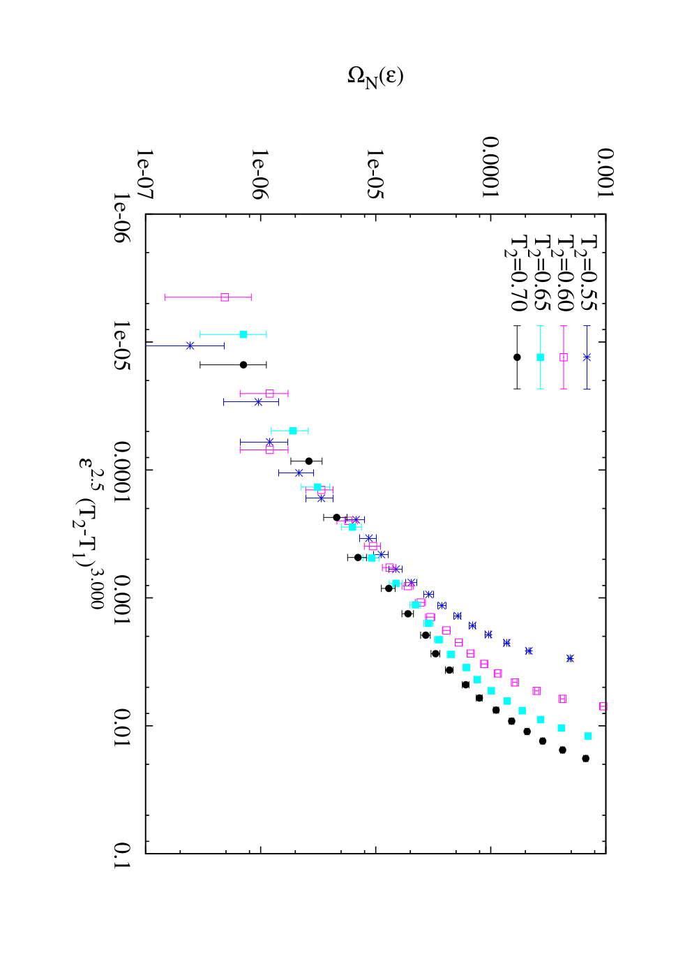
In a finite volume, temperature chaos weakens as $|T_{2}-T_{1}|$ decreases, and the onset of chaos is pushed to higher and higher values of $N$. It has been suggested [11] that for small $\epsilon$ and small temperature difference one has $\Omega^{N}_{0.4,0.6}(\epsilon)\propto\epsilon^{\beta}(T_{2}-T_{1})^{b}$ with $b\approx 1.8$ for the 3D EAI model. Our data for the SK model are compatible with such a scaling and a value $b\approx 3$, as show in Figure 3 for $N=4096$. Due to large statistical errors in the small $\epsilon^{\beta}(T_{2}-T_{1})^{b}$ region where scaling holds, this is only a rough estimate. An extreme numerical effort would be needed in order to pinpoint precisely the value of the exponents $\beta$ and $b$. A method to either enrich the tail of the sample distribution corresponding to low values of $q_{T1;T2}$ or to select the samples belonging to the tail before performing a lengthy Monte Carlo simulation would be of great help in this matter.

The analytical prediction [16, 17] for the SK model coupled replicas large deviation potential $\Delta F(q)$ is that $\beta=7/2$ and $b=2$, but subleading terms are present that cause transient effects in small volumes. This may explain the apparent discrepancy with our numerical results. Another possibility is that the exponents $\beta$ and $b$ are not the same for the potential $\Delta F(q)$ and the potential $\Omega(\epsilon)$ studied here.

In conclusion, we have reanalyzed our SK data using the new rare events based analysis method proposed in [11]. We find a clear signal for temperature chaos in the SK model, at the same evidence level as the results of [11] for the 3D EAI model. In both cases temperature chaos is best seen by analyzing individual quenched disorder samples: As $N$ grows, chaos first appears with rare samples that are very chaotic, chaotic samples are more numerous as $N$ keep on growing, asymptotically, for values of $N$ far beyond numerical reach, all samples are chaotic. The finite size scaling of the distribution of chaotic samples is encoded in a large deviation potential that scales as a function of overlap squared $\epsilon=q^{2}$ and temperature difference as $\Omega^{N}_{0.4,0.6}(\epsilon)\propto\epsilon^{\beta}(T_{2}-T_{1})^{b}$, and we give crude estimates of the values of the exponents $\beta$ and $b$.

References

- [1] A. J. Bray and M. A. Moore, Phys. Rev. Lett. 58, 57 (1987).
- [2] J. R. Banavar and A. J. Bray, Phys. Rev. B35, 8888 (1987).
- [3] D. S. Fisher and D. A. Huse, Phys. Rev. B38, 286 (1988).
- [4] M. Ney-Nifle and H. J. Hilhorst, Physica A193, 48 (1993).
- [5] M. Ney-Nifle and A. P. Young, J. Phys. A30, 5311 (1997).
- [6] M. Ney-Nifle, Phys. Rev. B57, 492 (1998).
- [7] F. Krzakala, Europhys. Lett. 66, 847 (2004).
- [8] M. Sasaki, K.Hukushima., H. Yoshino and H. Takayama, Phys. Rev. Lett. 95, 267203 (2005).
- [9] H. G. Katzgraber and F. Krzakala, Phys. Rev. Lett. 98, 017201 (2007).
- [10] C. Monthus and T. Garel, arXiv:1310.2815.
- [11] L. A. Fernandez, V. Martin-Mayor, G. Parisi and B. Seoane, EPL, 103, 67003 (2013).
- [12] D. Sherrington and S. Kirkpatrick, Phys. Rev. Lett. 35, 1792 (1975).
- [13] S. Kirkpatrick and D. Sherrington, Phys. Rev. B17, 4384 (1978).
- [14] A. Billoire and E. Marinari, J. Phys. A33, L265 (2000).
- [15] A. Billoire and E. Marinari, Europhys. Lett. 60, 775 (2002).
- [16] T. Rizzo and A. Crisanti, Phys. Rev. Lett. 90, 137201 (2003).
- [17] G. Parisi and T. Rizzo, J. Phys. A43, 235003 (2010).
- [18] I. Kondor, J. Phys. A22,L163 (1989).
- [19] I. Kondor and A. Végsö, J. Phys. A26, L641 (1993).
- [20] T Rizzo, J. Phys. A: Math. Gen. 34, 5531 (2001).
- [21] A. Billoire, L. A. Fernandez, A. Maiorano, E. Marinari, V. Martin-Mayor, G. Parisi, F. Ricci-Tersenghi, J. J. Ruiz-Lorenzo, D. Yllanes Phys. Rev. Lett. 110, 219701 (2013).