Bayesian Hypothesis Assessment in Two-arm Trials Using Relative Belief Ratios

Recently, hypothesis testing has been an active research topic in various types of two-arm clinical trials. As an example, a clinician may want to demonstrate whether a new treatment is not worse than that of a reference treatment (also known as active control or standard treatment) by more than a specified margin [1]. This helps in assessing whether a less toxic, easier to administer, or less expensive treatment, is medically noninferior to a reference treatment. This kind of clinical trial, where the intention is to demonstrate that the new treatment is not inferior to the standard treatment by more than a small predefined margin $\delta,$ is known as a noninferiority trial. Here $\delta>0$ is known as the prespecified clinically irrelevant or noninferiority margin. Two-arm noninferiority trials of a new treatment and a well established reference treatment are an attractive option as in certain settings they avoid exposing patients to placebo situations. There has been a series of articles on this topic; see for example, special issues of Statistics in Medicine (Volume 47, Issue 1, 2005) and Journal of Biopharmaceutical Statistics (Volume 14, Number 2, 2004).

Sometimes in clinical trials, the goal is not to show that the new treatment is better, but rather equivalent to the reference treatment. This kind of clinical trial is known as an equivalence trial [2]. In an equivalence trial, the aim is to show that new treatment and the reference treatment have equal efficacy. For practical purposes, one can select a margin $\delta$ such that two treatments can be considered not to differ when their true difference lies in the interval of clinical equivalence $(-\delta,\delta).$ Note that this is different from testing a difference between two treatments which is a two-sided test known as superiority test in clinical literature. In this case $\delta>0$ is called the clinically equivalence margin. Note that in either case, $\delta$ must be defined a priori.

There is a considerable literature on the related problems of hypothesis tests in clinical trials. As a simple frequentist method, one can use the standard $t$ test for testing these hypotheses. At a higher level a generalized p-value approach may be applied using a generalized test function [3]. One can also perform tests using the ratio of the averages instead of the difference between the averages [4, 5]. Bayesian non-inferiority tests for proportions in two-arm trials with a binary primary endpoint [6] and normal means [7] are also considered in recent literature.

This paper considers a novel Bayesian approach for assessing a hypothesis in two-arm trials using relative belief ratios. A relative belief ratio for a hypothesized value of a parameter of interest is interpreted as the evidence that the hypothesized value is correct. We may obtain evidence either for or against the hypothesized value. Associated with a relative belief ratio is a measure of the strength of this evidence and this may be weak, strong or inconclusive. General inferences based on relative belief ratios are developed in [8, 9, 10].

We discuss relative belief ratios and associated theory in Section 2 and illustrate this by application to the problem of interest. In Section 3 we consider the elicitation of the prior and how we can measure the suitability of the prior both with respect to its agreement with what the data say and with respect to measuring the bias a prior puts into the analysis. In Section 4, the approach is applied to a data set obtained from a two-arm clinical trial. We conclude with a short discussion in Section 5.

Suppose we have a statistical model, as given by a collection of densities $\{f_{\theta}:\theta\in\Theta\},$ and a prior $\pi$ on $\Theta.$ After observing data $x,$ the posterior distribution of $\theta$ is given by the density

where $m(x)=\int_{\Theta}\pi(\theta)f_{\theta}(x)\,d\theta.$ For an arbitrary parameter of interest $\psi=\Psi(\theta)$ we denote the prior and posterior densities of $\psi$ by $\pi_{\Psi}$ and $\pi_{\Psi}(\cdot\,|\,x),$ respectively. The relative belief ratio for a hypothesized value $\psi_{0}$ of $\psi$ is defined by

the ratio of the posterior to the prior at $\psi_{0}.$ As such, $RB_{\Psi}(\psi_{0})$ is measuring how beliefs have changed that $\psi_{0}$ is the true value from a priori to a posteriori. Considering the case when the prior for $\psi$ is discrete, we have that $RB_{\Psi}(\psi_{0})>1$ means that the data have lead to an increase in the probability that $\psi_{0}$ is correct, and so we have evidence in favor of $\psi_{0},$ while $RB_{\Psi}(\psi_{0})<1$ means that the data have lead to a decrease in the probability that $\psi_{0}$ is correct, and so we have evidence against $\psi_{0}.$ As discussed in [10], this interpretation is also appropriate in the continuous case via a consideration of limits.

Clearly relative belief ratios are similar to Bayes factors, as they are both measuring change in belief, but the Bayes factor does this by comparing posterior to prior odds while the relative belief ratio compares posterior to prior probabilities and so is somewhat simpler. In fact, in certain circumstances the relative belief ratio and Bayes factor can be considered as equivalent but this is not always true. The full relationship between these quantities is discussed in [10].

One problem that both the relative belief ratio and the Bayes factor share as measures of evidence, is that it is not clear how they should be calibrated. Certainly the bigger $RB_{\Psi}(\psi_{0})$ is than 1, the more evidence we have in favor of $\psi_{0}$ while the smaller $RB_{\Psi}(\psi_{0})$ is than 1, the more evidence we have against $\psi_{0}.$ But what exactly does a value of $RB_{\Psi}(\psi_{0})=20$ mean? It would appear to be strong evidence in favor of $\psi_{0}$ because beliefs have increased by a factor of 20 after seeing the data. But what if other values of $\psi$ had even larger increases? While calibrations of Bayes factors have been suggested [11, 12, 13] the proposed scales seem arbitrary and it is not at all clear that there is a universal scale on which Bayes factors or relative belief ratios can be calibrated.

A more useful calibration of (1) is given by

which is the posterior probability that the true value of $\psi$ has a relative belief ratio no greater than that of the hypothesized value $\psi_{0}.$ If we interpret $RB_{\Psi}(\psi_{0})$ as the measure of the evidence that $\psi_{0}$ is the true value, we see that (2) is the posterior probability that the true value has evidence no greater than that for $\psi_{0}.$

While (2) may look like a p-value, we see that it has a very different interpretation. For when $RB_{\Psi}(\psi_{0})<1,$ so we have evidence against $\psi_{0},$ then a small value for (2) indicates a large posterior probability that the true value has a relative belief ratio greater than $RB_{\Psi}(\psi_{0})$ and so we have strong evidence against $\psi_{0}.$ If $RB_{\Psi}(\psi_{0})>1,$ so we have evidence in favor of $\psi_{0},$ then a large value for (2) indicates a small posterior probability that the true value has a relative belief ratio greater than $RB_{\Psi}(\psi_{0})$ and so we have strong evidence in favor of $\psi_{0}.$ Notice that in the set $\{\psi:RB_{\Psi}(\psi)\leq RB_{\Psi}(\psi_{0})\},$ the ‘best’ estimate of the true value is given by $\psi_{0}$ simply because the evidence for this value is the largest in this set. Various results have been established in [10] supporting both (1), as the measure of the evidence and (2), as the strength of that evidence.

As a measure of the strength of the evidence, (2) seems to work best when the posterior probabilities for all the possible values of $\psi$ are all small or even 0 as in the continuous case. When some of these values have large posterior probabilities we can augment (2) as follows. If the prior $\pi_{\Psi}$ corresponds to a discrete distribution with $\pi_{\Psi}(\psi_{0})>0,$ we have that

The right-hand inequality holds generally, see [10], while the left-hand inequality requires discreteness. Suppose $\pi_{\Psi}(\psi_{0}\,|\,x)$ and (2) are both small and notice that this happens whenever $RB_{\Psi}(\psi_{0})$ is small. In this case we clearly have strong evidence against $\psi_{0}$ when $RB_{\Psi}(\psi_{0})<1$ and weak evidence for $\psi_{0}$ when $RB_{\Psi}(\psi_{0})>1.$ Also, when $\pi_{\Psi}(\psi_{0}\,|\,x)$ and (2) are both big, then we have only weak evidence against $\psi_{0}$ when $RB_{\Psi}(\psi_{0})<1$ and strong evidence for $\psi_{0}$ when $RB_{\Psi}(\psi_{0})>1.$

The other possibility is that the posterior probability $\pi_{\Psi}(\psi_{0}\,|\,x)$ is small and (2) is big. If the prior probability $\pi_{\Psi}(\psi_{0})$ is big and $RB_{\Psi}(\psi_{0})<1,$ then this suggests that we have indeed obtained strong evidence against $\psi_{0}$ because (2) is big only because there are many other values of $\psi$ for which there is evidence against $\psi$ at least as strong as the evidence against $\psi_{0}.$ If, however $\pi_{\Psi}(\psi_{0})$ is small and $RB_{\Psi}(\psi_{0})<1,$ then we have weak evidence against $\psi_{0}$ because $\pi_{\Psi}(\psi_{0}\,|\,x)$ is small due to $\pi_{\Psi}(\psi_{0})$ being small. When $\pi_{\Psi}(\psi_{0})$ is big and $RB_{\Psi}(\psi_{0})>1,$ then we must have $\pi_{\Psi}(\psi_{0}\,|\,x)$ is big as well, so no ambiguity arises, while when $\pi_{\Psi}(\psi_{0})$ is small, then again $\pi_{\Psi}(\psi_{0}\,|\,x)$ is small due to $\pi_{\Psi}(\psi_{0})$ being small and so in both situations we have strong evidence in favor of $\psi_{0}$ via (2). So the only context where (2) might not suffice as a measure of the strength of the evidence given by $RB_{\Psi}(\psi_{0}),$ is when $\psi$ has a discrete prior distribution with $\pi_{\Psi}(\psi_{0})$ a non-neglible size, $\pi_{\Psi}(\psi_{0}\,|\,x)$ small and (2) big. In general there is no harm in the discrete case in quoting (2), $\pi_{\Psi}(\psi_{0}\,|\,x)$ and $\pi_{\Psi}(\psi_{0}),$ as part of the analysis of the strength of the evidence given by $RB_{\Psi}(\psi_{0})$ and we recommend this.

There is another issue associated with using $RB_{\Psi}(\psi_{0})$ to assess the evidence that $\psi_{0}$ is the true value. One of the key concerns with Bayesian inference methods is that the choice of the prior can bias the analysis in various ways. For example, in many problems Bayes factors and relative belief ratios can be made arbitrarily large by choosing the prior to be increasingly diffuse. This phenomenon is known as the Jeffreys-Lindley paradox because a diffuse prior is supposed to represent less information.

An approach to dealing with this paradox is discussed in [10]. Given that we accept that $RB_{\Psi}(\psi_{0})$ is the evidence that $\psi_{0}$ is true, the solution is to measure a priori whether or not the chosen prior induces bias either for or against $\psi_{0}.$ To see how to do this we note first the Savage-Dickey result, see [14] and [10], which says that

where

is the prior-predictive density of the data $x$ given that $\Psi(\theta)=\psi_{0}.$ Actually, it is easy to see that, if $T(x)$ is a minimal sufficient statistic for the full model, then $m(x\,|\,\psi_{0})/m(x)=m_{T}(T(x)\,|\,\psi_{0})/m_{T}(T(x))$ where $m_{T}$ is the prior predictive density of $T$ and $m_{T}(\cdot\,|\,\psi_{0})$ is the prior predictive density of $T$ given that $\Psi(\theta)=\psi_{0}.$

From (4) we can measure the bias in the evidence against $\psi_{0}$ by computing

as this is the prior probability that we will obtain evidence against $\psi_{0}$ when $\psi_{0}$ is true. So when (5) is large we have bias against $\psi_{0}.$ To measure the bias in favor of $\psi_{0}$ we choose values $\psi_{0}^{\prime}\neq\psi_{0}$ such that the difference between $\psi_{0}$ and $\psi_{0}^{\prime}$ represents the smallest difference of practical importance. We then compute

as this is the prior probability that we will obtain evidence in favor of $\psi_{0}$ when $\psi_{0}$ is false. Again, when (6) is large we have bias in favor of $\psi_{0}.$ Note that both (5) and (6) decrease with sample size and so, in design situations, they can be used to set sample size and so control bias.

When we are not able to control sample size, then (5) and (6) can be computed and used to qualify any conclusions we reach about whether $\psi_{0}$ is true or not. For example, if we have evidence against $\psi_{0}$ and (5) is large, this has to be taken with a ‘grain of salt’ as our choices have biased things this way. We draw a similar conclusion if we have evidence in favor of $\psi_{0}$ and (6) is large. Of course, these negative conclusions could also lead us to redo the analysis using a prior that does not induce such biases when this is possible, see Section 3.

A variety of other inferences can be derived from interpreting $RB_{\Psi}(\psi)$ as the evidence that $\psi$ is the true value. For example, the best estimate of $\psi$ is clearly the value for which the evidence is greatest, namely,

and called the least relative surprise estimator in [8, 9, 10]. Associated with this is a $\gamma$-credible region

where

Notice that $\psi_{LRSE}(x)\in C_{\gamma}(x)$ for every $\gamma\in[0,1]$ and so, for selected $\gamma,$ we can take the size of $C_{\gamma}(x)$ as a measure of the accuracy of the estimate $\psi_{LRSE}(x).$ Given the interpretation of $RB_{\Psi}(\psi)$ as the evidence for $\psi,$ we are forced to use the sets $C_{\gamma}(x)$ for our credible regions. For if $\psi_{1}$ is in such a region and $RB_{\Psi}(\psi_{2})\geq RB_{\Psi}(\psi_{1}),$ then we must put $\psi_{2}$ into the region as well as we have at least as much evidence for $\psi_{2}$ as for $\psi_{1}.$

In [8, 9, 10] various optimality properties are established for $\psi_{LRSE}(x)$ and the regions $C_{\gamma}(x)$ in the class of all Bayesian inferences. One notable property is that inferences based on the relative belief ratio are invariant under reparameterizations. This is not the case for Bayesian inferences based on losses, such as the posterior mean or mode and highest probability density regions.

We now consider the application of relative belief inferences to two-arm trials.

Let $x_{E}=(x_{E,1},\ldots,x_{E,n_{E}})$ denote the sample from the experimental treatment and $x_{R}=(x_{R,1},\ldots,x_{R,n_{R}})$ denote the sample from the reference treatment. We assume that these responses are mutually independent with $x_{E,i}\sim N(\mu_{E},\sigma^{2})$ and $x_{R,i}\sim N(\mu_{R},\sigma^{2})$ where $\mu_{E},\mu_{R}\in R^{1}$ and $\sigma^{2}>0$ are all unknown. The information in the data is summarized by the minimal sufficient statistic $T(x_{E},x_{R})=(\bar{x}_{E},\bar{x}_{R},s^{2})$ where $s^{2}=[(n_{E}-1)s_{E}^{2}+(n_{R}-1)s_{R}^{2}]/(n_{E}+n_{R}-2)$ and the likelihood equals

We will use the prior for $(\mu_{E},\mu_{R},\sigma^{2})$ given by

We will discuss elicitation of the hyperparameters $\mu_{0},\tau_{0}^{2},\alpha_{0}$ and $\beta_{0}$ in Section 3. The posterior distribution of $(\mu_{E},\mu_{R},\sigma^{2})$ is then easily obtained and is given by

Note that it is simple to generate values from (8) and (9).

Now suppose we want to assess the hypothesis that the true value of $\mu_{E}-\mu_{R}$ satisfies ${|\mu_{E}-\mu_{R}|<\delta.}$ So ${\delta}$ represents a practically meaningful difference between the means. If the difference is less than this quantity, then we do not distinguish between $\mu_{E}$ and $\mu_{R}$ but otherwise we do. It makes sense then that, if $\mu_{E}$ and $\mu_{R}$ do differ, we would want to know how many units of ${\delta}$ these means differed by. So for the $\psi$ parameter of interest in this problem we will consider $\psi\in\mathbb{Z}$ where $\psi=i$ indicates that ${\mu_{E}-\mu_{R}\in((2i-1)\delta,(2i+1)\delta].}$ So the hypothesis of interest corresponds to $H_{0}:\psi=0.$

To calculate the relative belief ratios for values of $\psi$ we need the prior and posterior distributions of this parameter. These quantities are obtained by discretizing the prior and posterior distributions of ${\mu_{E}-\mu_{R}.}$ We have that the marginal prior distribution of ${\mu_{E}-\mu_{R}}$ is given by

and the marginal posterior distribution of ${\mu_{E}-\mu_{R}}$ is given by

where $\nu=n_{E}+n_{R}+2\alpha_{0}-4$ and

When $\nu$ is large, the posterior distribution is approximately normal, while it has heavy tails when $\nu$ is small.

So to assess $H_{0}$ the evidence is given by

and the strength of the evidence is given by

Both (12) and (13) are easily evaluated using the exact distribution theory given for the prior and posterior distribution of ${\mu_{E}-\mu_{R}.}$ For example, we can use the $t$ distribution function routine in the R software package.

Suppose that we obtain $RB_{\Psi}(0)<1$ and that (13) indicates that this is reasonably strong evidence against $H_{0}.$ From the tabulation of $RB_{\Psi}(i),$ that we computed as part of calculating (13), we easily obtain the optimal estimate of $\psi,$ namely,

If $\psi_{LRSE}(x_{E},x_{R})$ is greater than 0, then we have a clear indication that the experimental treatment is better than the reference treatment. The accuracy of the estimate is assessed by computing the $0.95$-relative belief region

and seeing how large it is. We can convert this into a region for ${\mu_{E}-\mu_{R}}$ via

To assess the bias in the prior we have to compute (5) and (6). From (10) and (11) we can evaluate

and note that $RB_{\Psi}(0)$ depends on the data only through $(\bar{x}_{E}-\bar{x}_{R},s^{2}).$ We then need only simulate from the conditional prior predictive of $(\bar{x}_{E}-\bar{x}_{R},s^{2})$ given that $\psi$ is the true value. Note that, given $(\mu_{E}-\mu_{R},\sigma^{2})$ then

and these quantities are independent.

We can compute (5) by the following simulation process:

1. 1.

   set a counter $C=0,$

2. 2.

   generate $\sigma^{2}$ using (8),

3. 3.

   generate $\mu_{E}-\mu_{R}$ from a $N(0,2\tau_{0}^{2}\sigma^{2})$ distribution conditioned to
   $-{\delta<\mu_{E}-\mu_{R}\leq\delta,}$

4. 4.

   generate $(\bar{x}_{E}-\bar{x}_{R},s^{2})$ using (14),

5. 5.

   compute $RB_{\Psi}(0)$ and add 1 to $C$ if it is less than 1,

6. 6.

   repeat 2-4 $N$ times and record $C/N$ as the estimate of (5).

The only slightly difficult part in this simulation is step 3 and for that we can use an inversion algorithm. For denoting the cdf and inverse cdf of a $N(0,1)$ distribution by $\Phi$ and $\Phi^{-1},$ respectively, we generate $\mu_{E}-\mu_{R}$ in step 3, when conditioning on ${(2i-1)\delta<\mu_{E}-\mu_{R}\leq(2i+1)\delta,}$ by generating $u\sim U(0,1)$ and putting

We can use routines in $R$ for $\Phi$ and $\Phi^{-1}$ to evaluate (15).

In any statistical analysis a statistician chooses a model that supposedly describes the generation of the data and, in a Bayesian analysis, also chooses a prior. As the analysis is typically highly dependent on these subjective choices, it is important that they be checked against what is typically objective, at least if it is collected correctly, namely, the data.

We illustrate the approach described in Sections 2 and 3 using a data set published in [2]. The data come from a comparative trial of moxonodin and captopril in the antihypertensive treatment of patients suffering from major depression. The response variable is the reduction of diastolic blood pressure, measured in millimeters of mercury (mm Hg), of patients suffering from a major depression under two drugs captopril (experimental) and moxonodin (reference). The data is given by

so $n_{E}=n_{R}=12.$ The minimal sufficient statistic of the data is $T(x_{E},x_{R})=(\bar{x}_{E},\bar{x}_{R},s^{2})=(7.21,4.17,46.79).$ We suppose that a practically meaningful difference in the means is given by $\delta=0.5$ mm Hg.

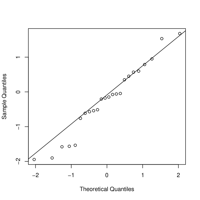
Figure 1 gives the Q-Q plots of the residuals. The Shapiro-Wilks test for normality applied to the residuals gives a p-value of $0.51.$ This indicates that the data is not inconsistent with the normality assumption with constant variance.

For prior elicitation, we initially propose to reflect vague knowledge about the parameters by choosing a very diffuse prior. The values $m_{1}=-100,m_{2}=100,s_{1}^{2}=5$ and $s_{2}^{2}=1000$ lead to the hyperparameter values

The bias in this prior is assessed by computing (4) and (5) with $\psi_{0}=0$. We found that

indicating that there is very little bias against $\psi_{0}.$ We see, however, that

and this indicates that we have considerable bias in favor of $\psi_{0}$. This is undoubtedly because we have chosen the prior to be too diffuse. Using such a prior will lead us to overstate the evidence in favor of the hypothesis or equivalently, understate the evidence against.

So to avoid the bias as much as possible, we chose different values for the hyperparameters. For this we set $m_{1}=-20,m_{2}=20,s_{1}^{2}=10$ and $s_{2}^{2}=600$ which lead to the hyperparameter values

In this case we get

indicating that there is some bias both for and against the hypothesis with this choice of prior. We cannot expect to be able to get both of these values to be low as this is controlled by sample size and we do not have a lot of data.

We checked this prior using (22) and (23). The value $0.15$ was obtained for (22) and the value $0.22$ obtained for (23). This indicates that there is no reason to be concerned about prior-data conflict.

Figure 2 contains a plot of the posterior and relative belief ratio for the continuous parameter. For the discretized parameter $\psi$ we obtained $RB_{\Psi}(0)=0.515$ with a strength of $0.19.$ As such we have only moderately strong evidence against the hypothesis of equivalence. Also

and the $0.95$-relative belief region is given by

The length of this interval indicates a fair degree of uncertainty about the true value but we do have reasonable evidence that the treatments are not equivalent.

Note that $C_{0.95}^{\ast}(x_{E},x_{R})$ includes the value 0 but this is not a contradiction with the fact that we have evidence against $\psi=0.$ These credible regions do not work like confidence intervals do with p-values. It is only the length of $C_{0.95}^{\ast}(x_{E},x_{R})$ that is relevant as a measure of the accuracy of the estimate $\psi_{LRSE}(x_{E},x_{R}).$ It is easily deduced from (7), and as discussed in [10], that there is a relationship between relative belief regions and the strength of the evidence (2). This makes sense as both are measuring the accuracy or reliability of inferences based on the measure of evidence as given by the relative belief ratio.

We investigated the choice of many other priors. The results were fairly consistent in obtaining evidence against $\psi=0$ and with similar strengths. The biases did vary considerably with sometimes there being very low bias against $\psi=0$ but accompanied by high bias in favor or conversely. Interestingly, such extreme cases are often accompanied by prior-data conflict.

Alternatively, we could assess the hypothesis of noninferiority, namely, $H_{0}:\psi\in(-{\delta,\infty)}$ for which $\Pi((-{\delta,\infty)})=0.58$ and $\Pi((-{\delta,\infty)}\,|\,x_{E},x_{R})=0.89.$ Therefore,

indicates evidence in favor of $H_{0}$ being true. Since the posterior probability of $H_{0}$ is large, this indicates strong evidence in favor of the experimental treatment being at least as effective as the reference treatment.

We have considered the application of relative belief inferences to an important inference problem with two-arm clinical trials. This is seen to provide a clear definition of what the evidence is, whether in favor of or against, for a hypothesis. Moreover, with such a definition this allows us to assess the bias introduced into a statistical analysis by a proper prior and so addresses a key concern with the use of Bayesian inference methods. In addition we have provided a methodology for eliciting an appropriate prior in such a context and demonstrated how one checks this prior to see if it is contradicted by the data.

In general, we take the view that all of statistics is subjective as we choose sampling models and priors and possibly even choose other ingredients. Such subjectivity is always present in a statistical analysis. Rather than searching for methods that are supposedly ‘objective’ in some sense, we embrace the subjectivity as allowing us to make judgements that reflect additional information we have about the application. Once the model and prior are chosen, we can go forward and make inference, based on the measure of statistical evidence and its calibration, in an unambiguous way. If we want these inferences to be convincing, however, it is important that we check the ingredients chosen against that aspect of the analysis that can best be claimed to be objective, namely, the data. So model checking and checking for prior-data conflict are essential parts of any statistical analysis. The analysis in this paper is presented as a meaningful application of this approach to statistical analyses.

In Section 3.3 the prior predictive density of $V=(n_{E}+n_{R}-2)s^{2}$ is

Suppose $U=(U_{1},U_{2})\,|\,\sigma^{2}\sim N_{2}(\mu,\sigma^{2}\Sigma)$ where $\sigma^{2}$ is distributed as in (8). Then the marginal density of $U$ is