Is the Higgs Boson Associated with
Coleman-Weinberg Dynamical Symmetry Breaking?
Abstract
The Higgs mechanism may be a quantum phenomenon, i.e., a Coleman-Weinberg potential generated by the explicit breaking of scale symmetry in Feynman loops. We review the relationship of scale symmetry, trace anomalies, and emphasize the role of the renormalization group in determining Coleman-Weinberg potentials. We propose a simple phenomenological model with “maximal visibility” at the LHC containing a “dormant” Higgs doublet (no VEV, coupled to standard model gauge interactions ) with a mass of GeV. We discuss the LHC phenomenology and UV challenges of such a model. We also give a schematic model in which new heavy fermions, with masses GeV, can drive a Coleman-Weinberg potential at two-loops. The role of the “improved stress tensor” is emphasized, and we propose a non-gravitational term, analogous to the -term in QCD, which generates it from a scalar action.
pacs
14.80.Bn,14.80.-j,14.80.-j,14.80.DaI. Introduction
The discovery of a light Higgs boson presents several well-known puzzles: “What mechanism determines the mass of the Higgs boson?” “What is the custodial symmetry that yields a small mass scale for the apparently pointlike particle?” “Is there any new associated dynamics with the Higgs boson?” These questions revolve around the problem of the naturalness of the existence of a low mass fundamental spin- field in quantum field theory.
Supersymmetry offers solutions to these problems. The custodial symmetry of light Higgs bosons could be the chiral symmetry of their superpartners, e.g., the fermionic Higgsinos. This, however, requires proximity in mass scale of SUSY states and, so far, supersymmetry has not emerged in searches. SUSY is also highly constrained by the relatively heavy GeV Higgs boson mass, and indirect measures, such as the electron EDM and , etc.. While SUSY remains a popular candidate for an ultimate solution to these problems, its relevance to the electroweak scale has become somewhat clouded by the necessity of a high degree of fine-tuning [1, 2, 3, 4]. SUSY as the custodial symmetry of the Higgs boson will be subject to more definitive tests in Run-II of the LHC, circa 2015-18.
Strong dynamics also offers natural solutions, by postulating a mechanism similar to that of QCD for electroweak symmetry breaking (see the review, [5]). QCD involves explicit breaking of scale symmetry via the trace anomaly, proportional to the -function of the QCD coupling constant. The QCD mass scale, which accounts for the masses of the nucleons and, hence, most of the visible mass in the universe, is an example of mass generation by “dimensional transmutation.” This is inherently a quantum phenomenon, i.e., it is mass generated from quantum mechanics itself. The QCD hierarchy arises naturally since the ratio of the QCD scale , to any large scale in nature, , is given:
| (1) |
where at one-loop precision. Here one inputs a small dimensionless coupling constant, , at an arbitrary high energy scale, . Quantum loops then generate the small ratio, . Eq.(1) implies that the ’t Hooft naturalness, i.e., the custodial symmetry associated with the smallness of the ratio, , which occurs when , has the interpretation of the classical scale symmetry of QCD in the limit [6, 7].
Straightforward attempts to implement an analogous QCD-like mechanism for generating the weak scale have generally failed. This approach typically yields light boundstates, e.g., Nambu-Goldstone techni-pions. These couple perturbatively to and , through axial anomalies, and therefore cannot be imposters of a Higgs boson which couples at tree level and is consistent with present experimental indications. There is effort underway to construct viable scenarios (for a partial list, see e.g., refs.[8, 9, 10, 11, 12, 13]), but strong dynamical models, as a class, have been even more severely constrained by LHC data than SUSY.
The present evidence from the LHC strongly favors a simple perturbative Higgs boson interpretation of the data as proposed by Weinberg in 1967 [14]. But to date we have no understanding as to the origin of the electroweak scale, first introduced by Fermi in 1934 [15].
Presently we wish to focus upon an alternative approach. We will argue for a quantum origin of the Higgs potential and electroweak scale: We propose that the Higgs potential is a perturbative Coleman-Weinberg potential [16]. As such, we ask what the current data might be telling us and what might be visible consequences of this hypothesis at the LHC in Run-II and beyond [17]. We emphasize at the outset that we will not delve in great detail into the UV completion aspects of this idea. We think the question, “Is the Higgs potential generated by quantum mechanics?” to be sufficiently compelling that it should be posed in a self-contained framework, and addressed experimentally in Run-II and beyond.
Coleman-Weinberg (CW) symmetry breaking is complimentary to a QCD-like, strong dynamical mechanism. It arises from a stress-tensor trace anomaly, i.e., it relies upon scale symmetry breaking by perturbative quantum loops. This means that CW symmetry breaking can be understood entirely in terms of the renormalization group (RG) running of the the Higgs scalar quartic coupling constant, in analogy to QCD. We discuss this in greater formal detail in Section II and Appendices A-C and we’ll introduce a few new ideas.
With a CW potential the custodial symmetry for the weak scale again arises like QCD, as the scale invariance of the action in the limit. In this limit quantum loops are turned off and the trace anomaly goes to zero. The “improved stress tensor,” [18], defines the renormalization group of the CW potential, and the trace anomaly is determined as . We see that is the anomalous dimension of the potential. CW symmetry breaking occurs at a local minimum of the potential, where the anomalous dimension takes on the value and the potential operator becomes pure vacuum energy.
The CW potential, expanded about its minimum, depends only upon the local values of RG -functions and their derivatives. We give an expression valid to all orders in perturbation theory, through quintic order in the Higgs field, for the CW potential. Incidently, in Appendix A we introduce a novel, non-gravitational term, into the scalar field action that is a non-topological analogue of the -term in QCD, but which generates the improved stress tensor from variation of the action.
The idea that classical scale symmetry can arguably serve as a custodial symmetry of a fundamental perturbative Higgs boson has been emphasized by Bardeen [19, 6]. In implementation of the CW mechanism to obtain the observed value of GeV and Higgs boson mass, GeV, we find, in its simplest and most obvious incarnation, that additional large bosonic contributions to the RG equation for the Higgs quartic coupling are required. Recently, various authors have focused on related models, many of which accomplish this with bosonic dark matter fields, [20, 21, 22, 23, 24]. We will presently examine a “maximally visible new physics scenario at LHC” to implement the CW mechanism. We will also propose a novel mechanism for generating a CW potential from fermions that emerges upon a more detailed scrutiny of the RG (see Section V).
In Sections III and IV we consider a bosonic model consisting of a second, “dormant,” Higgs boson as the source of new bosonic contributions to the RG equations to sculpt the CW potential. Here we distinguish the oft-used term “inert doublet,” to imply that the second Higgs doublet does not interact with standard model gauge fields, (e.g., as in the dark matter models of [21, 22, 23, 24]), from the term “dormant Higgs doublet.” By “dormant” we imply that the second doublet does interact with standard interactions, however the second doublet has no VEV. Such dormant Higgs doublet models are valid solutions to the original Weiberg-Glashow natural, [25], two-Higgs doublet schemes [26, 27]. Our question is: “How accessible is the dormant Higgs doublet at the LHC?” We estimate production and decay rates and, modulo a more thorough LHC detector based analysis, the results are encouraging.
Phenomenologically, we find that the new dormant Higgs doublet must have a mass of about GeV. Since we assume standard model couplings, it is guaranteed to be pair-produced, above threshold of GeV, via and at the LHC. Other production and decay channels are likely, but model dependent. We think it is most natural, albeit an additional assumption, that the dormant doublet couples to quarks, with a large coupling constant, . This makes the dormant doublet the natural flavor partner of the Higgs with it’s large coupling to the top quark. These -quark couplings allow enhanced production of single and in association with and or , and would also imply decays like and which become interesting observables at the LHC.
One intriguing corollary associated with the CW potential is that the Higgs potential will have cubic, quadrilinear, even quintic (and higher order) coupling constants, that will be significantly different than those of the standard model [17, 23].
In Section V we also present a schematic model of a Coleman-Weinberg potential for the Higgs generated by new fermions. This is a novel approach, and arises from a two-loop effect in the RG structure of the CW potential. We think this class of models may alleviate some of the potential problems encountered with new heavy bosons in UV completion, which requires further development [32]. While we have not examined the full UV structure or phenomenological implications of this scheme, it suggests pair produced new fermions with masses GeV. These fermions would have their own strong interaction, and may be produced in boundstates with a threshold at GeV, or pairs of new heavy meson-like boundstates at GeV.
We begin by discussing some general theoretical aspects of Coleman-Weinberg symmetry breaking.
II. General Theoretical Considerations
.1 Schematic Analysis
To get a feeling for how Coleman-Weinberg symmetry breaking works, with particular emphasis upon the renormalization group (RG), we consider a Higgs scalar field potential . This classical potential, for has an uninteresting minimum at as in Fig.(1).
A process with Feynman loops is of order in field theory. Quantum loops lead to the RG running of couplings, such as , with scale, . Typically, we might have a one-loop, , solution to the RG equations as in Fig.(2):
| (2) |
where . simply parameterizes the particular RG trajectory of the running , i.e., we would ask our experimental colleagues to measure the dimensionless quantity at some energy scale , and we would then choose so that we fit their result as .


With the running quartic coupling constant, the scale can be set by the vacuum expectation value, , of the field itself. The resulting scalar potential, as a function of , is then:
| (3) |
This potential has a local minimum, as in Fig.(3), at . A stable minimum of the potential, i.e., one with a positive curvature at the minimum, or , occurs just below the zero-crossing of from a negative to a positive value. Hence must be negative and must be positive at the minimum (we’ll see in Section V that there are alternative solutions involving two loops in which the situation is flipped, i.e., () can be negative (positive)).
If continues to run as , we would see that the ratio of the VEV, , to any other scale is then:
| (4) |
A large hierarchy between and can be exponentially controlled by the ratio of dimensionless quantities, . With , the ’t Hooft naturalness of the “small ratio” of , or , would be, in analogy to QCD, associated with the limit , which is again the limit of classical scale invariance, . Of course, the RG running of can be complicated over a large range of .
, which we have approximated as a constant above, is the -function of which defines the Gell-Mann–Low renormalization group equation [28]:
| (5) |
To see the structure of the CW potential in somewhat greater detail we expand the potential of eq.(3) in about a hypothetical vacuum expectation value :
| (6) |
where is a physical Higgs boson field, according to :
| (7) | |||||
We thus have the CW Higgs potential:
| (8) | |||||
The extremum of the potential is given by:
| (9) |
which requires:
| (10) |
The Higgs boson mass is then given by:
| (11) |
If the extremum is to be a minimum we must impose the positivity condition:
| (12) |
Therefore, from equation (10):
| (13) |
This shows that and at the minimum of the potential (we’ll see in Section V that there is a flipped solution arising at two-loops with and ).
The resulting Higgs potential, expanded about the minimum and using eq.(10) through quintic order, is:
| (14) | |||||
.2 All-Orders RG Improved Potentials
The above analysis of the CW Higgs potential is schematic, relying upon a particular solution and expanding in a leading logarithm. In Section II.C we’ll see that the trace anomaly of the “improved stress tensor” implies an exact equation for the Coleman-Weinberg potential of a scalar field :
| (15) |
We can view this as the definition of the CW potential for the VEV of . Here is the all-orders function of . The solution is:
| (16) |
(the normalization is locked to the definition of the classical potential, and defines ). This is formal, but a useful application to the previous model of Section II.A, with , applies to both CW and standard model Higgs potentials, involves the expansion of in terms of the -functions computed to all-orders of perturbation theory in all relevant couplings.
We label all relevant coupling constants that enter in any order of the loop diagrams for the running of (e.g., , , , etc.) as . We denote the scalar quartic (Higgs) coupling as with -function . Each has its own :
| (17) |
The derivatives of about the VEV can be written in terms of the -functions:
| (18) | |||||
| (19) | |||||
| (20) | |||||
| (21) | |||||
(we tabulate the quintic order in Appendix D). Each is a function of the couplings, , evaluated at the scale, . We use the summation convention for repeated indices, .
The leading terms in the CW potential now take the form to all orders in :
| (22) | |||||
The extremum condition is therefore formally the same as in the schematic case:
| (23) |
but note that this is now an all-orders in condition and, likewise, the anomalous dimension of the potential when we impose the extremum is to all orders.
Imposing the extremum condition, eq.(23), we obtain the Coleman-Weinberg potential expanded about the energy minimum:
| (24) | |||||
(the quintic term, , is tabulated in Appendix D). As a check on these results, notice that if we keep only the leading terms, we recover the schematic model case of eq.(8).
Note that we can also apply this expansion to the standard model:
| (25) | |||||
Here we use to designate the SM quantities which generally differ from the CW quantities. Eq.(25) is a “low energy theorem” for the SM Higgs potential in a limit in which the Higgs boson is considered an approximate dilaton [31]. We have retained a quintic term to remind the reader that the standard model will have such terms, and beyond, owing to the RG running of .
Remarkably, we see that the Coleman-Weinberg potential expanded about its minimum, , depends only upon -functions and their derivatives at , i.e., is wholly determined by the renormalization group. Of course, we have swapped for , having used the extremal condition, , to eliminate . The standard model has an input mass, and therefore we cannot eliminate the separate and dependences. We will use the improved potentials for comparson of the trilinear, quartic and qunitic terms below.
.3 Role of the “Improved Stress tensor”
Here we emphasize the underlying canonical aspects of the dynamical Coleman-Weinberg potential and renormalization group, in part to give a formal basis to the idea of couplings that run with field VEVs and a derivation of eq.(15). [A reader interested only in our phenomenological model can skip this section and go directly to Section III. The material is summarized here, and is developed in greater detail in Appendix A.]
The canonical stress tensor of a real scalar theory with potential is:
| (26) |
The “scale current,” the Noether current associated with scale symmetry, takes the form , and divergence is given by . These are defined and derived in Appendix A.
The problem now arises that the canonical stress tensor has a nonvanishing trace, , even for a scale invariant theory. Yet, we see that the trace represents breaking of scale symmetry since it is the divergence of the scale current. Therefore, an “improved” stress-tensor for scalar fields, was introduced by Callan, Coleman and Jackiw [18]:
| (27) | |||||
The scale current now takes the form . and the trace is found to be:
| (28) |
where we’ve used the equation of motion, . Classically, is then traceless for a potential of the form , where is a constant, reflecting the exact classical scale invariance of the theory. The improved stress-tensor is therefore required to discuss the scale symmetry of scalar fields.
The stress tensor is derived canonically from a scalar field action by performing a coordinate variation, called a “diffeomorphism.” It can alternatively be derived by performing a variation of the background metric. The improved stress tensor is generally viewed as emerging from a scalar field action, , which includes the gravitational “conformal coupling term,” with , and is given by . However, there must exist, for symmetry reasons, another way of obtaining the same improved stress tensor without considering the metric variation.
In Appendix A we provide a modified scalar field action which generates while maintaining a fixed flat-space metric. Such a “dual derivation” of exists because of the defining gauge symmetry of general relativity, general (Einstein) covariance: if we simultaneously do the diffeomorphism and the covariant metric variation (i.e., the particular metric variation under the diffeomorphism as dictated by general covariance) then the action must be invariant 11 1 This dual derivation of the conserved current is fundamental to any gauge theory, and is analogous to the fact that the electromagnetic current can be obtained by locally varying the vector potential in the Dirac action, , or by varying the phase of the electron wave-function, . Doing both at the same time with is just a gauge transformation, under which the Dirac action is invariant.. The modifed action that generates the improved stress tensor in flat space has an additional term, one that is a total divergence, . This term, albeit non-topological, is similar to a -term in QCD, undergoes a nontrivial variation when we perform the flat-space diffeomorphism. It generates a correction, which adds to the canonical stress tensor and yields the improved stress tensor. The term remains a surface term when the metric is non-flat, and it does not affect either the equations of motion, or any local variation of a non-flat metric.
When the matrix elements of the operator are evaluated at the quantum loop level for the classically scale invariant theory, they are found to be nonzero at , taking the operator value:
| (29) |
Eq.(29) is the RG equation for the potential . The rhs is the “trace anomaly” and it reflects the breaking of scale symmetry. [We carry out a Feynman loop evaluation of the trace anomaly in Appendix B. We also reproduce the classic Coleman-Weinberg potential for massless scalar electrodynamics using the RG in Appendix C, and discuss some of its subtleties.]
Formally we see that we can represent the trace anomaly when the RG running of as a function of is incorporated. By “” we mean the VEV, or a soft classical field configuration. We have from eq.(28) when combined with eq.(5) with :
| (30) |
The RG running of with is essential to represent the anomalous result in the low energy effective theory. This is much like the representation of the chiral anomaly by shifts in pNGB’s, e.g., the pion or gauge fields, in a Wess-Zumino-Witten (WZW) term: The running coupling constant scalar potential plays the analogous role for scale symmetry anomalies that the WZW term plays for chiral anomalies. In the WZW term the axial anomaly is represented entirely bosonically, i.e., the pion shift under a chiral transformation generates the axial anomaly. We emphasize that the trace anomaly is an explicit, not spontaneous, breaking of scale symmetry and there is no associated Nambu-Goldstone boson, i.e., there need be no dilaton here [31].
.4 The trace anomaly is the “anomalous dimension” of the potential
Eq.(29) informs us that the ratio is indeed the anomalous dimension of the potential. This must become large, to manufacture mass from no mass. In fact, the condition that the induced potential has an extremum, hence a local minimum, is precisely that of eq.(10):
| (31) |
This result is true to all orders in a perturbation theory in as we’ve seen Section II.B. At the extremal point in field space the potential is converted to , which corresponds to vacuum energy, i.e., a cosmological constant.
If dimensional transmutation is to occur, we see that the condition implies that an quantity, , is being equated to an coupling constant . This would seemingly violate perturbation theory. However, if there are additional coupling constants beyond that appear in , e.g., , then the ratio can easily be much greater than unity, while maintaining perturbativity, and the relationship eq.(31) can consistently occur. This is at the heart of the Coleman-Weinberg phenomenon, as emphasized in their paper [16].
III. Phenomenological Model of the Higgs Boson Potential
We now wish to apply the above apparatus to a model of the Higgs potential. For simplicity, first consider the Higgs and top quark subset of the standard model:
| (32) |
where . The one-loop RG equation for is [33]:
| (33) |
where we neglect the electroweak couplings presently (we include these below).
Let us approximate as a constant in the SM. Note that, using the phenomenological values and , we infer from eq.(33):
| (34) |
is positive in the standard model, and is negative. However, as we’ve seen in the previous section, if we want a CW effective potential for the Higgs we require a negative value of and a positive .
Numerically, if a CW potential is to fit the observed Higgs boson, we would require:
| (35) |
To make large and positive to requires more bosonic degrees of freedom [6].
Perhaps the simplest and most natural model for a CW potential of the Higgs boson is to introduce a heavy second Higgs doublet, . With a new Higgs doublet we have additional cross-coupling terms . The most general classically scale invariant potential with two massless Higgs doublets and “Weinberg-Glashow naturalness” is well known [25],[26],[27]:
| (36) | |||||
By judicious choice of parameters we can have one Higgs, develop a VEV, while remains dormant, i.e., no VEV.
The potential of eq.(36) has a “Higgs parity” symmetry . Without couplings to fermions, additional Higgs doublets are therefore stablized by this symmetry, and would become stable dark matter. Our present goal, however, is to maintain reasonable visibility of the second doublet at the LHC and we therefore require that can decay into visible final states.
Weinberg and Glashow [25] noted that such a parity symmetry amongst the Higgs multiplets alone, can be broken by couplings to fermions, but then a larger reflection symmetry can exist where sets of the coupled right-handed fermions are also reflected, e.g., , . The overall symmetry can be maintained if we allow one new doublet per right-handed charge species in the standard model. This suppresses flavor changing neutral Higgs boson couplings at tree-level that would otherwise threaten such things as the small mass difference of the , but it now allows to decay into the fermions it couples to.
For visibility at the LHC the parity symmetry must therefore be broken via coupling to fermions, but the overall symmetry of Weinberg-Glashow maintained as much as possible. However, is dormant, so the fermions coupled to it exclusively cannot then get mass. We therefore ultimately require some small breaking of the overall Weinberg-Glashow symmetry.
There are two possibile schemes: (A) We can have the couple, with possibly a large coupling constant, to , respecting Weinberg-Glashow symmetry, but with its smaller SM coupling to allowing to be generated by the VEV; (B) we can add new “centi-weak” bosonic terms to the Higgs potential that break the parity symmetry.
In scheme (A) all quarks and leptons couple to just as they do to the standard model Higgs, and acquire mass via the VEV. We postulate that the -quark, however, also has a large coupling to ,
| (37) |
where and (the choice of -quark, as opposed to other down quarks, is a modelling assumption, motivated to maintain a symmetry). We are therefore slightly violating the Weinberg-Glashow symmetry. This then raises the question: “Are we now in trouble with flavor constraints, such as ?” Not definitively, but the full analysis of the flavor physics of this scheme is beyond the scope of the present paper. There is, however, always an escape route that was employed in “topcolor” models: we can assume flavor textures, such as in [34], where essentially the CKM matrix arises via the “up” type quarks, and the Higgs couplings of “down” types are diagonal. This suppresses any large flavor changing neutral Higgs mediated transitions. In any case, a more detailed analysis of flavor constraints is warranted. Certainly the model survives in the limit where the Weinberg-Glashow symmetry is recovered, but gluon fusion associated production of at the fb level will then turn off, while EW production at the fb level remains (see IV.(A)).
Alternatively, in scheme (B) all quarks and leptons couple to as in the standard model, and acquire mass via the VEV, but we have no coupling of quarks to to the -quark. Here the down quarks coupled only to , which maintains the Weinberg-Glashow symmetry. We then break this symmetry by introducing a bosonic interaction:
| (38) |
(of course, this new interaction would be induced by fermion loops involving down-quarks, if they coupled to both and ). Since this interaction also breaks Weinberg-Glashow naturalness, we therefore expect to be small.
The bosonic interaction of eq.(38) leads to an interesting effect that may explain the flavor hierarchy between and charge species. When the Higgs acquires a VEV, it induces a tadpole interaction to the neutral component of ,
| (39) |
where . is initially dormant and will acquire a large positive mass from the VEV, . But, through the tadpole, we obtain a small induced VEV for :
| (40) |
The down quarks will then have small induced masses, and . The interaction eq.(38) also splits the neutral and charged members of the dormant doublet.
In scheme (B) the dormant Higgs will have decay modes via eq.(38) such as , and/or , etc., and radiative modes , etc.. These are interesting modes to search for, but their detailed analysis is beyond the scope of the present paper and require further study. We will focus here upon the phenomenology of scheme (A).
The general RG equations for two-doublet models are given in ref.[33]. We introduce fermionic couplings and we choose as a starting point Model IV as defined in [33]. We assume operationally that couples to the top quark via and couples to the quark via (we ignore all other smaller Higgs-Yukawa couplings),
| (41) |
where and .
We’ve analyzed many variations of this model with , , and all active. Presently we’ll discuss only the simplest case with . breaks a global symmetry, , , and is therefore multiplicatively renormalized. Hence, it remains zero once set to zero, and this is evident in the RG equation above for . Moreover, in the absence of and ignoring the the gauge fields, we see that breaks a larger symmetry, , and it too is then multiplicatively renormalized. If is set to zero at some high scale, it therefore remains reasonably small and can be ignored.
Let’s estimate the required effect of needed to create the Coleman-Weinberg potential for . We have at one-loop order from eq.(24):
| (47) |
hence:
| (48) |
From eq.(42) we also have:
| (49) | |||||
which yields:
| (50) |
(We use GeV, GeV, GeV, so ; also , ). While this is a rather large coupling, it is still perturbative, as its contribution to the .
When the Higgs, , acquires its VEV the term of the potential, eq.(36), will induce a mass for , . We require that the dormant doublet have a positive and therefore, is positive. We thus estimate:
| (51) |
With such a large we can improve the prediction by including the two-loop effect of eq.(24). The Higgs mass is given by
| (52) |
where the second term arises at two-loop level. We can use the leading dependence upon the large in the last term. From eq.(42)
| (53) |
hence,
| (54) |
(note that which is the scale of these higher order corrections is small). Solving again for , we now obtain:
| (55) |
Of course, the large leads to a “UV challenge” for this scheme. Since is large, it’s RG running into the UV leads to a Landau pole. Indeed, we see this from a numerical integration of eqs.(42) in Figure (4). We have considered the effects of the additional couplings, and and have not found an elegant or simple remedy to this problem without a significant extension of the model.
We note that we can somewhat improve the UV behavior of this scheme by considering to be a QCD color triplet, , and . In this structure then form a bosonic generation, similar to a lepton-quark generation, with . can then couple to a quark-lepton combination, e.g. or . thus becomes a “lepto-quark.” The case is intriguing, as we would integrate it out as in neutrino Majorana masses, and then becomes dark matter.
We can drastically modify the scheme to push the Landau pole upwards in energy scale, by imbedding at some high energy scale, , below the Landau pole. This is analogous to “top-flavor” models [35], and can be done in a flavor democratic way. The effect is to replace with a larger in the RG equations. This improves the UV behavior. Landau poles generally reflect compositeness of fields [11]. The compositeness conditions are associated with the vanishing of wave-function normalization constants, .

IV. Phenomenology of
(A) Production and Decay of the Dormant Higgs
We have carried out estimates of decay widths and production cross-sections of the dormant doublet, , using CalcHEP. We’ve adapted the “inert doublet model,” with inclusion of the Yukawa couplings to the -quark (see [36]). Since our goal was to maintain “maximal visibility” of the new bosons that allow a Coleman-Weinberg potential for the Higgs, is necessarily coupled to the gauge fields of the standard model. The doublet does not have a VEV, but (ignoring fermion couplings ) the neutral components, which we denote as and , are pair-produced via , ; the charged components are likewise pair-produced via .
We follow the conventional nomenclature of the SUSY two doublet schemes, but we emphasize that the minimal theoretical scheme maintains an approximate degeneracy between and , and , hence the doublet is defined as . The degeneracy is broken by the Yukawa couplings to matter, , where . New quartic interactions that lift the degeneracy by way of the normal Higgs boson VEV (which is the neutral member of ) will be induced by fermion loops. Throughout we have assumed the degenerate doublet with GeV.
| Process | value | comments | |
|---|---|---|---|
| GeV | |||
| GeV | |||
| absent in model | |||
| fb | |||
| absent in model | |||
| fb | |||
| absent in model | |||
| or | fb | ||
| fb | |||
| fb | |||
| fb | |||
| fb | |||
| or | pb | No cuts | |
| fb | and GeV | ||
| fb | and GeV | ||
| fb | No cuts | ||
| fb | , GeV | ||
| fb | , GeV | ||
| fb | No cuts | ||
| fb | GeV | ||
| fb | GeV |
In principle could exist with no coupling to matter. However, as described in the previous section, we will allow a large coupling to the -quark. As such, the neutral and can then be pair produced in association with , and the charged in association with and .
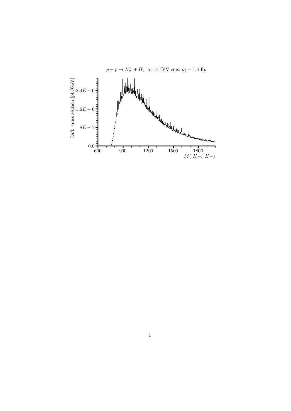
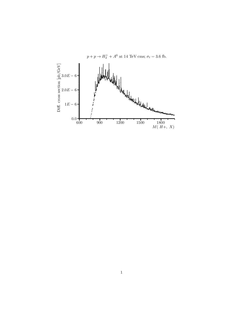
The decay widths , and are then generated and computed in Table I. Note that in our minimal scheme a parity that would make the components stable is broken only by the Yukawa coupling to . Therefore, at tree level the decays , are absent in the model. The decay widths are of order GeV for . The distributions for these processes are indicated in Figs.(5,6).
The SM gauge production cross-sections are computed for the LHC RUN-II at TeV. While small, fb, these may be observable with fb-1 of data and judicious cuts.
We have also computed the model dependent ( associated production rates for , and . These are predominantly gluon fusion processes at the LHC. We have applied various cuts as indicated on final state particles, but we have not done a detailed signal/background analysis, requiring more careful detector dependent study.
(B) Trilinear, Quadrilinear, and Quintic Higgs Coupling
A characteristic feature of the Coleman-Weinberg potential is that the trilinear, quadrilinear and quintic Higgs couplings differ dramatically from that of the standard model [17], [23].
With the standard model polynomial potential we have:
| (56) | |||||
From the Coleman-Weinberg potential expanded to quintic order, keeping the leading two-loop terms, we have:
| (57) | |||||
The ratios of the Coleman-Weinberg to standard model trilinear, quadrilinear and quintic terms are then:
| trilinear | ||||
| quadrilinear | ||||
| quintic |
where is the SM -function for . The leading terms in the above, independent of the new bosonic physics are valid to , while the are the leading largest terms.
The sensitivity at the LHC Run II is expected to be comparable to these departures from the standard model, and in future high-luminosity mode these effects should be observable with precision. Future Higgs factories would have sensitivity at the level of or better.
While this is a model independent check on the “Higgs with CW potential” scheme we are considering, it is not the case in other models. For example, in [21] the second doublet is inert, and does not couple to the standard model . The second doublet couples to a new gauge interaction and develops a large VEV. The new gauge fields together with become a dark matter ecosystem. In this model the Higgs acquires a negative mass2 via a negative (“Higgs portal interaction”), and the resulting potential is classical. There would be no large trilinear effect in this model, and it is presumably hard to test this scheme at the LHC.
V. Fermionic Origin of a CW Higgs Potential
Remarkably, the full structure of eq.(24) admits an alternative origin of a Coleman-Weinberg potential for the Higgs boson via fermions. This exploits the two-loop contribution to the term. We will presently give a schematic discussion of this possibility, but it requires more model building effort which we will pursue elsewhere [32].
Suppose there exists a new fermion doublet , and a pair of singlets . Hence the fermion couples to the standard model , gauge bosons while has only weak hypercharges. We further assume these new fermions are “hyperquarks,” forming an fundamental representation, coupled to an unbroken strong gauge interaction, , “hypercolor,” with coupling constant . We’ll ignore the issue of anomaly cancellation presently.
We assume the charges are so chosen that the interaction with a massless Higgs boson can occur as:
| (59) |
and we’ll assume a common Yukawa coupling (we’ll work in the approximation of custodial invariance).
The Higgs boson is massless but has the usual quartic potential with RG equation for dominated by the Higgs-Yukawa term [33]:
| (60) | |||||
where we’ve neglected the top Yukawa, and electroweak contributions. Likewise, the RG equation for the Yukawa coupling takes the form [33]:
| (61) |
The Higgs potential can develop a dynamical minimum for a VEV, , provided that:
| (62) |
Previously we have studied that case where and . We will now discuss a case with the new fermions in which and , and we assume at some that eq.(62) holds.
A stable minimum of the potential requires . From eq.(24), including the two-loop term, we see that:
| (63) |
Using the approximate form of eq.(60) we have:
| (64) |
hence,
| (65) | |||||
The condition that is positive is now the simultaneous conditions of eq.(62) and:
| (66) |
The latter condition states that the anomalous dimension of the Higgs-Yukawa interactions eq.(59) is less than and thus the dimensionality of this operator is reduced to . Eq.(66) can be realized by
| (67) |
where . The subsequent running of the hypercolor into the infrared is model dependent. With additional inert fermion flavors (not coupled to ), will blow up at a scale , and confine. This could in principle be a walking theory. With the minimal , we see that . We prefer a limit so that the masses of the states are far above the confining scale of hypercolor, and no chiral condensates are formed.
The Higgs mass at the minimum is therefore given by:
| (68) |
If we assume and we find that the masses of the new hyperquarks are GeV.
Note that these objects would appear effectively as new leptons since they do not interact with ordinary QCD , and are not produced in gluon fusion. Hypercolor could be QCD-like and confine at some scale . We assumed that this is less that the inferred Higgs-induced masses, GeV of ; therefore the resulting states are analogues of heavy quark-onium boundstates in QCD, and there are no light pNGB’s.
The new states will be pair produced via a single or at a threshold , into a single heavy meson, (plus recoil jets of conventional quarks). The heavy decays into electroweak gauge bosons. Open requires the the recombination into pairs of mesons, and a threshold energy of .
Using fermions to engineer the CW potential may allow a much more natural UV completion than the bosonic model presented above. The detailed model structures, production and decay phenomenology is beyond the scope of the present discussion. Our interest here is to give a proof of principle of the phenomenon of fermion-driven Coleman-Weinberg potentials.
VI. Conclusions
We have discussed the possibility that the electroweak scale is a quantum phenomenon, i.e., that it arises via particle loops leading to a perturbative Coleman-Weinberg potential. We have developed the renormalization group formalism for the Coleman-Weinberg potential, and its relationship to the trace anomaly of the improved stress tensor for scalar fields. An expansion of the CW potential about its minimum, valid to all orders of perturbation theory, is also described and suggests new possibilities for the underlying dynamics.
We have surveyed the possibility that the observed Higgs boson with a Coleman-Weinberg potential is maximally observable at the LHC. To achieve this we assume a minimal extension of the standard model consisting of a second, “dormant,” Higgs doublet that couples to the standard model gauge fields. The dormant Higgs doublet can sculpt a Coleman-Weinberg potential for the Higgs boson provided it has a mass of about GeV.
The new doublet, coupled to standard model , is pair produced at the LHC in and at the fb level. It can naturally couple strongly to some SM fermions, and we consider the case of coupling to the b-quark. In this case the production can be via gluon fusion with to fb cross-sections. The coupling to the fermions, albeit model dependent, is essential to make visible final states at the LHC. In the cases considered we are encouraged that the new states may be observable in Run-II at the LHC.
The departures from the standard model Higgs potential, the trilinear, quadrilinear and even quintic self-couplings, are fairly significantly modified in this scenario, and may also be addressable at the LHC, and certainly at future Higgs factories.
We have also described a schematic model in which the CW potential arises at the two-loop level via new fermions. These would have masses at the order of GeV, and would be pair produced at the LHC. We will develop this idea further elsewhere.
The general idea that “the Higgs mass comes from quantum mechanics” is, to us, sufficiently compelling to warrant the present phenomenological approach and ask if there is any evidence, potentially visible to experiment, that can determine whether the CW mechanism is operant for the Higgs boson. As such, our focus has presently largely left the UV completion issues untouched.
Yes, there are certainly challenges and difficulties in constructing a UV complete scenario (see, e.g., [29, 30]). The main problem with our simple phenomenological model is the occurance of nearby Landau poles in the running quartic couplings, that are reached at TeV. These are either blemishes on the scheme, or may be harbingers of new physics, such as compositeness of the new bosonic states, [10, 11, 13, 12]. We’ve only briefly discussed UV completion issues, as we feel these issues are secondary. We plan to return to these issues in greater detail elsewhere [32].
If we could establish a Coleman-Weinberg origin of the Higgs boson mass, we would then have two scales in nature generated by quantum loop effects: and . The grand hypothesis that: “all mass in nature comes from quantum mechanics” would gain significant validation. Our view of the UV would then have to accomodate it. This hypothesis may ultimately imply a radically different view of nature than our current “GUTs to strings” philosophy.
Some of these issues and “predictions” have been discussed elsewhere [7]. For example, we live in a universe, and it is striking that is the only possibility for classical scale symmetry given Yang-Mills field theories as an underpinning of nature, since the trace of the Yang-Mills field stress tensor is classically zero only in . Quantum mechanics then supplies the trace anomaly and allows for the generation of mass and large hierarchies through the renormalization group. We see this with QCD and the compelling question is whether it also applies to the weak scale and Higgs boson. Hence, the hypothesis that “all mass in nature comes from quantum mechanics” already seems broadly consistent with our , large universe. The stakes are high: this may ultimately require a classically scale-invariant approach to gravity, such as Weyl gravity with a quantum, QCD-like origin of [37] (see also [7] and references therein).
Acknowledgements
I wish to thank for useful discussions, K. Allison, W. Bardeen, E. Eichten, H. Frisch, G. G. Ross, P. Steinhardt, R. Vidal, C. Wagner, and various members of the ATLAS collaboration, particularly J. Allison and D. Miller.
Appendix A: Scalar Field Stress Tensors
Consider a scalar field theory in flat spacetime with Minkowski metric :
| (A.1) |
where the Euler-Lagrange equation of motion is:
| (A.2) |
We perform an infinitesimal diffeomorphism in the flat space theory holding the metric fixed:
| (A.3) |
where the scalar field is invariant, 22 2 Note that here we can define and hence , and no additional terms are generated; alternatively we can do an active tranformation and additional terms are generated but vanish by integration by parts and use of equations of motion., but the coordinate differentials transform as:
| (A.4) |
The action transforms as:
| (A.5) | |||||
and the resulting canonical stress tensor is:
| (A.6) |
Note the divergence of the stress tensor:
| (A.7) | |||||
The stress tensor is the Noether current associated with translations in space and time. The conservation of the stress tensor is a consequence of these symmetries and implies the equation of motion.
We can choose, however, , corresponding to an infinitesimal scale transformation. The action then varies as:
| (A.8) |
and the scale current is defined by:
| (A.9) |
with divergence:
| (A.10) |
The canonical stress tensor, however, has a nonzero trace, even when is scale invariant.
| (A.11) |
It can be “improved” to yield a vanishing trace in the scale invariant case, e.g., when [18].
Stress Tensor Improvement
We add to the action a total divergence:
| (A.12) |
where can be viewed as an arbitrary function of space-time, but we take the limit (constant) after manipulating the action. With constant this is a surface term and does not affect the equations of motion. However, it varies under the diffeomorphism to produce a nonvanishing result:
| (A.13) | |||||
Note that the second term in the (constant) limit is an irrelevant surface term, but the first and third terms yield:
| (A.14) | |||||
where:
| (A.15) |
has the trace:
| (A.16) |
We thus choose and obtain the “improved stress tensor”:
| (A.17) | |||||
The conservation of the stress tensor is unaffected by adding the conserved improvement term . However, we see that the trace now yields:
| (A.18) |
We can also generate the improved stress tensor by including the“conformal coupling” of the scalar field to gravity, in the action:
| (A.19) |
In weak field gravity the metric is expanded about the flat Minkowski metric:
| (A.20) |
and to :
| (A.21) |
where: (signs are tricky here).
We choose and the first order action becomes:
| (A.22) | |||||
Hence, a small variation in the metric about flat spacetime, , generates the improved stress tensor with the inclusion of the conformal term.
Note that the term does not affect the local metric variation in curved space since:
| (A.23) |
where is the covariant derivative. We see that this is a surface term and is insensitive to a local variation .
We’ve seen that the variation of the action in flat space by the diffeomorphism, generates the improved stress tensor in the presence of the term. Likewise a variation of the metric generates the improvement with the conformal coupling term. An Einstein transformation (general covariance) implies:
| (A.24) |
If we perform both of these transformations together we obtain:
| (A.25) |
which is zero when eq.(A.24) is applied. This is now a gauge transformation. The diffeomorphism on the “matter side” cancels the variation wrt the metric on the “gravity side”, and both transformations generate a conserved improved stress tensor. This is analogous to any gauge theory, such as QED, where we can generate the current by doing a local gauge transformation of the electron wave-function ( “matter side”) or by varying the action wrt the vector potential ( “gravity side”). We can define the Noether current for scale symmetry by either procedure.
Appendix B. Trace Anomaly and Feynman Loops
A classically scale invariant potential is defined by the condition:
| (B.1) |
For a classically scale invariant potential the improved stress tensor trace, eq.(A.18), vanishes, and the associated scale current is conserved.
In general, where is the “anomalous dimension” of the potential. Such is the case for Coleman-Weinberg potentials where the running of the coupling is included. For example, if we choose,
| (B.2) |
then we see:
| (B.3) |
This is called the trace-anomaly; is the anomalous dimension.
Let us examine how the trace anomaly arises at the one-loop level via a direct calculation of the effective potential. Consider the real scalar field theory lagrangian:
| (B.4) |
We define renormalized couplings and counterterms:
| (B.5) |
The counterterms can be computed from the 1PI scattering amplitudes of Figs.(7A, 7B). We obtain:
| (B.6) |
Here we define the Feynman loops with Euclidean momentum space cut-off and neglect external momenta in the loops. There is no wave-function renormalization constant as there is no external momentum flow through the loop of Fig.(7A) i.e., the theory is super-renormalizeable.
We use the expansion and work in a classical background field, . We introduce a classical source term in the lagrangian, . This induces the shift in the field,
| (B.7) |
where satisfies the renormalized equation of motion, 33 3 The reason for introducing the source term is to remove all the linear cross-terms, , arising from the shift. In this perturbative approach there remain terms, . These we ignore since we are working to . We then add back a term which cancels the arising from the shift. The general formalism of the Legendre transformed potential is given in ref.([16]). . The lagrangian becomes:
| (B.8) |
where, to :
| (B.9) |
and:
| (B.10) | |||||
where the refers to terms of higher order in .

We now integrate out the quantum fluctuations, . Let be the path integral. The effective lagrangian becomes , which takes the form:
| (B.11) | |||||
Note that the second term acquires a sign flip since . We drop irrelevant additive constants.
The integral can be done by performing a Wick rotation (, , and ) and we use a Euclidean momentum space cut-off, . Up to additive constants , we obtain:
If we now add in the counterterms of eq.(B.6) as in eq.(B.11) we have:
| (B.13) |
where the effective potential is:
| (B.14) |
where:
| (B.15) |
The classically scale invariant limit corresponds to . The potential then becomes:
Note that there is an infrared divergence in the limit and we retain the in the argument of the log as an infrared regulator.
We can now constuct the improved stress tensor from the full effective lagrangian eq.(B.13):
| (B.17) | |||||
The equation of motion of is now and includes the quantum effects,
| (B.18) |
The trace of the improved stress tensor is therefore:
where the latter term arises from the derivative of the logarithm in eq.(.4).
Note that we can infer the -function of from in eq.(B.6). With our sign convention, , and we can identify the “running RG scale” with , hence :
| (B.20) |
Comparing expressions we thus see that the trace anomaly is:
| (B.21) |
We therefore observe that, for a theory with vanishing renormalized mass, , we have a violation of scale symmetry by the trace anomaly, , which is and represents the RG running ot . We have no other such source of scale violation in this limit. There are, of course, infrared singularities in higher order terms in the expansion, for , but these are associated with the long-distance physics of the matrix element of the trace anomaly operator itself.
The important implication of this result, as emphasized by Bardeen, [6, 19], is that the additive quadratic divergence needed to renormalize the mass is an artifact of our calculational procedure and has nothing to do with the physics of mass generation. The scale current and its divergence controls the physics of mass generation. A scale invariant field theory is one whose scale current is strictly conserved to all orders in perturbation theory; a classically scale invariant theory will typically experience scale breaking by the trace anomaly, but the additive quadratic divergence, , encountered in the calculational procedure is a red herring.
Appendix C: Classic Coleman-Weinberg Potentials from the Renormalization Group
There are various renormalization groups. The relevant RG depends upon the application. For example, running a set of coupling constants in external momenta for scattering amplitudes, such as the QCD coupling with a single scale , is a typical application. Particles such as the top quark then decouple at , and the -function counts only the active light quarks below that scale, and this affects the evolution of and contributes to the value of .
In applications to the CW potential we are interested in running of coupling constants where the scale is replaced by the field, , itself. Here we are only including the low momentum components of , in particular the zero-momentum VEV of . If is the standard model Higgs boson, with its classical mass term set to zero, we want to vary over a large range of scales to find a minimum of the effective potential. Since the top quark receives its mass from this VEV, then the top quark never decouples as we run to lower values. The same is true for any field, such as , that receives its mass from the VEV of .
This is a surprising and counter-intuitive effect: if we were to run down to the QCD scale, for example, the QCD coupling would run with as well, but the top quark (and and quarks as well) would remain active far into the infrared. This has the stunning effect of reducing to about half of its normal value. Of course, the QCD chiral phase transition would still occur, at about GeV, and the resulting chiral breaking would occur, with 35 Nambu-Goldstone pions, and a QCD constituent quark mass would be generated for all 6 quarks. The Higgs doublet has the control VEV, , and this yields three additional massles NGB’s. These would mix with some of the pions, three of which would be eaten to break the electroweak symmetry. This is a dynamically stable “minimum of the Higgs effective potential” and it is similar to the way in which QCD would act as technicolor if there were no Higgs boson in the standard model.
Let’s consider in greater detail the direct derivation of Coleman-Weinberg potentials using the renormalization group. As an exercise, comparing to the derivation of ref.[16], we’ll use the RG method to derive the potential for massless scalar electrodynamics:
| (C.1) |
The RG equation for the quartic coupling is:
| (C.2) |
Note that this is similar to the RG equation for for a single Higgs boson in the standard model, as in [33], eq.(6a). The term, has become since the coefficient is where for a Higgs doublet and for a complex singlet , and for the real scalar field as we discussed above. The other terms are obtained by setting and where the factor is the weak hypercharge.
Consider the classical effective potential:
| (C.3) |
and we again obtain by solving the RG equation. We thus obtain in leading order where on the rhs and are approximated as constants:
| (C.4) |
To compare to ref.[16], eq.(4.5), we note the CW normalization conventions,
| (C.5) |
thus . We are consistent in the and terms with their result, ref.[16] eq.(4.5):
| (C.6) |
where
We see one discrepancy in the presence of the term in eq.(C.4) which is absent in eq.(C.6). The term arises for us because we have enforced the canonical wave-function normalization (kinetic term normalization) in our definition of i.e., canonical wave-function normalization is implict in our RG equation. To this order, however, we can absorb away the term by a field redefinition and it therefore does not affect the potential. We then identically reproduce the exact form of CW eq.(C.6).
We also see, however, that the term is irrelevant since we can absorb an additional factor into . With the net redefinition:
| (C.7) |
the resulting effective potential then contains only two relevant terms, the classical quartic coupling and the interaction term:
| (C.8) |
Indeed, as discussed by ref.[16], the only possible non-trivial perturbative minima of the effective potential involves exclusively these two terms. Moreover, the rescaled RG equation takes the form:
| (C.9) |
We also see that the RG admits a solution in which can be negative and cross to positive values with positive . The Landau pole occurs at and is is determined by the condition that the wave-function of is vanishing:
| (C.10) |
This form of the potential makes contact with the functional integral calculation where the photon mass is :
| (C.11) |
where the sum counts the spin states of the photon. Note that the massive contribution is not counted in this normalization. If we had not absorbed away the term we would find a mismatch in the coefficient of the term with the usual log path integral result. The RG equation is counting degrees of freedom in the symmetric phase, while the result counts only the real scalar (“Higgs”) degree of freedom and not the eaten Nambu-Goldstone modes (which are counted in the factor of 3 for the massive photon). The mismatch is present in general in this term, but is irrelevant for perturbative Coleman-Weinberg potentials.
We finally remark that for applications to dynamical situations, such as slow-roll inflationary models, it would be a blunder to ignore the wave-function renormalization terms, and one should adopt the canonically normalized form of the potential as in eq.(C.4). The slow-roll physical field motion is defined by the canonical normalization, so predictions of obervables may depend upon maintaining the canonical normalization.
Appendix D: Quintic Order terms in the Coleman-Weinberg Potential
The fifth derivative of the quartic coupling is:
| (D.1) | |||||
This leads to the quintic order contribution to the Coleman-Weinberg potential:
| (D.2) | |||||
References
- [1] See e.g., D. M. Ghilencea and G. G. Ross, Nucl. Phys. B 868 (2013) 65.
- [2] S. Cassel, D. M. Ghilencea and G. G. Ross, Nucl. Phys. B 835, 110 (2010).
- [3] A. Delgado, M. Garcia and M. Quiros; arXiv:1312.3235 [hep-ph].
- [4] H. Baer, V. Barger, P. Huang, D. Mickelson, A. Mustafayev and X. Tata, Phys. Rev. D 87, 115028 (2013).
- [5] C. T. Hill and E. H. Simmons, Phys. Rept. 381, 235 (2003) [Erratum-ibid. 390, 553 (2004)].
- [6] W. A. Bardeen, “On naturalness in the standard model,” Fermilab-Conf-95-391-T, and private communication.
- [7] C. T. Hill, “Conjecture on the physical implications of the scale anomaly,” hep-th/0510177, presented at M. Gell-Mann 75th birthday celebration, Santa Fe, (2005).
- [8] T. Appelquist and F. Sannino, Phys. Rev. D 59, 067702 (1999); O. Antipin, M. Mojaza and F. Sannino, “Natural Conformal Extensions of the Standard Model,” arXiv:1310.0957 [hep-ph]; R. Foadi, M. T. Frandsen and F. Sannino, Phys. Rev. D 87, 095001 (2013).
- [9] R. Shrock, “Studies on the UV to IR Evolution of Gauge Theories and Quasiconformal Behavior,” arXiv:1305.4572 [hep-ph].
- [10] V. A. Miransky, M. Tanabashi and K. Yamawaki, Phys. Lett. B 221, 177 (1989); ibid, Mod. Phys. Lett. A 4, 1043 (1989).
- [11] W. A. Bardeen, C. T. Hill and M. Lindner, Phys. Rev. D 41, 1647 (1990).
- [12] H. S. Fukano, M. Kurachi, S. Matsuzaki and K. Yamawaki, “Higgs as a Top-Mode Pseudo,” arXiv:1311.6629 [hep-ph]; Y. Aoki, et al., “A light composite scalar in eight-flavor QCD on the lattice,” arXiv:1309.0711 [hep-lat].
- [13]
H. -C. Cheng, B. A. Dobrescu and J. Gu,
arXiv:1311.5928 [hep-ph],
R. S. Chivukula, B. A. Dobrescu, H. Georgi and C. T. Hill, Phys. Rev. D 59, 075003 (1999),
B. A. Dobrescu and C. T. Hill, Phys. Rev. Lett. 81, 2634 (1998); - [14] S. Weinberg, Phys. Rev. Lett. 19, 1264 (1967).
- [15] E. Fermi, Z. Phys. 88, 161 (1934).
- [16] S. R. Coleman and E. J. Weinberg, Phys. Rev. D 7, 1888 (1973).
- [17] Much of this work was presented by the author in: C. T. Hill, “Profound Implications of the Higgs Boson,” US Atlas Physics Workshop, July 15, 2013, ANL, https://sites.google.com/site/usatlasphysicsworkshop2013/, and seminars at the ANL Theory Group, U. of Chicago, and Fermilab, (Fall, 2013).
- [18] C. G. Callan, Jr., S. R. Coleman and R. Jackiw, Annals Phys. 59, 42 (1970).
- [19] W. A. Bardeen, “Beyond Higgs,” Fermilab-Conf-08-118-T.
- [20] L. Alexander-Nunneley and A. Pilaftsis, JHEP 1009, 021 (2010); J. S. Lee and A. Pilaftsis, Phys. Rev. D 86, 035004 (2012).
- [21] T. Hambye and A. Strumia, Phys. Rev. D 88, 055022 (2013),
- [22] T. Hambye and M. H. G. Tytgat, Phys. Lett. B 659, 651 (2008),
- [23] R. Dermisek, T. Jung, H. Kim, arXiv:1308.0891 [hep-ph].
- [24]
R. Barbieri, L. J. Hall and V. S. Rychkov,
Phys. Rev. D 74, 015007 (2006);
L. Lopez Honorez, E. Nezri, J. F. Oliver and M. H. G. Tytgat,
JCAP 0702, 028 (2007);
J. R. Espinosa and M. Quiros,
Phys. Rev. D 76, 076004 (2007);
A. Arhrib, R. Benbrik and N. Gaur,
Phys. Rev. D 85, 095021 (2012);
K. Ishiwata,
Phys. Lett. B 710, 134 (2012);
C. D. Carone and R. Ramos,
Phys. Rev. D 88, 055020 (2013);
T.G. Steele and Zhi-Wei Wang, Phys. Rev. Lett 110 (2013) 151601,
T. G. Steele, Z. -W. Wang, D. Contreras and R. B. Mann, arXiv:1310.1960 [hep-ph];
V. Elias, R. B. Mann, D. G. C. McKeon and T. G. Steele, Nucl. Phys. B 678 (2004) 147 [Erratum-ibid. B 703 (2004) 413];
F. A. Chishtie, D. G. C. McKeon and T. G. Steele, Phys. Rev. D 77 (2008) 065007;
F. A. Chishtie, T. Hanif, J. Jia, R. B. Mann, D. G. C. McKeon, T. N. Sherry and T. G. Steele, Phys. Rev. D 83 (2011) 105009; A. Farzinnia, H.-J. He and J. Ren, Phys. Lett. B 727, 141 (2013); C. Englert, J. Jaeckel, V. V. Khoze and M. Spannowsky, JHEP 1304, 060 (2013); V. V. Khoze and G. Ro, JHEP 1310, 075 (2013); V. V. Khoze, JHEP 1311, 215 (2013); M. Holthausen, J. Kubo, K. S. Lim and M. Lindner, JHEP 1312, 076 (2013); R. Foot, A. Kobakhidze, K. L. McDonald and R. R. Volkas, arXiv:1310.0223 [hep-ph]; E. Gabrielli, M. Heikinheimo, K. Kannike, A. Racioppi, M. Raidal and C. Spethmann, arXiv:1309.6632 [hep-ph]; M. Aoki, S. Kanemura and H. Yokoya, Phys. Lett. B 725, 302 (2013). - [25] S. L. Glashow and S. Weinberg, Phys. Rev. D 15, 1958 (1977).
- [26] See page 100 of: C. T. Hill, “Higgs Scalars and the Nonleptonic Weak Interactions,” Caltech dissertation, June (1977); http://thesis.library.caltech.edu/4505/; the general non--invariant two-doublet scheme appeared earlier: P. Sikivie, Phys. Lett. B 65, 141 (1976).
- [27] N. G. Deshpande and E. Ma, Phys. Rev. D 18, 2574 (1978).
- [28] M. Gell-Mann and F. E. Low, Phys. Rev. 95, 1300 (1954).
- [29] C. H. Llewellyn Smith and G. G. Ross, Phys. Lett. B 105, 38 (1981).
- [30] G. Marques Tavares, M. Schmaltz, W. Skiba, Phys. Rev. D 89, 015009 (2014).
- [31] W. D. Goldberger, B. Grinstein, W. Skiba, Phys. Rev. Lett. 100, 111802 (2008).
- [32] C. T. Hill, and G. G. Ross, work in progress.
- [33] C. T. Hill, C. N. Leung, and S. Rao, Nucl. Phys. B262, (1985) 517.
- [34] G. Buchalla, G. Burdman, C. T. Hill and D. Kominis, Phys. Rev. D 53, 5185 (1996).
- [35] D. J. Muller and S. Nandi, Nucl. Phys. Proc. Suppl. 52A, 192 (1997); J. C. Lee, K. Y. Lee and J. K. Kim, Phys. Lett. B 424, 133 (1998); H. -J. He, T. M. P. Tait and C. P. Yuan, Phys. Rev. D 62, 011702 (2000); E. Malkawi, T. M. P. Tait and C. P. Yuan, Phys. Lett. B 385, 304 (1996).
- [36] A. Semenov, “LanHEP - a package for automatic generation of Feynman rules from the Lagrangian. Updated version 3.1,” arXiv:1005.1909 [hep-ph].
- [37] see, e.g., S. L. Adler, Rev. Mod. Phys. 54, 729 (1982) and refs. therein; E. Tomboulis, Phys. Lett. B 97, 77 (1980). This is a renormalizeable, theory of gravity that generates in a QCD-like way, where Einstein gravity is recovered as the low energy effective theory, in analogy to a chiral lagrangian of mesons for QCD. Research into Weyl gravity was largely superceded by superstring theory in 1984. String theory, however, assumes a classical input mass, the string constant, and is a priori hard to reconcile with the hypothesis of classical scale invariance and mass generated by quantum loops.