Convex Optimization for Binary Classifier Aggregation in Multiclass Problems
Abstract
Multiclass problems are often decomposed into multiple binary problems that are solved by individual binary classifiers whose results are integrated into a final answer. Various methods, including all-pairs (APs), one-versus-all (OVA), and error correcting output code (ECOC), have been studied, to decompose multiclass problems into binary problems. However, little study has been made to optimally aggregate binary problems to determine a final answer to the multiclass problem. In this paper we present a convex optimization method for an optimal aggregation of binary classifiers to estimate class membership probabilities in multiclass problems. We model the class membership probability as a softmax function which takes a conic combination of discrepancies induced by individual binary classifiers, as an input. With this model, we formulate the regularized maximum likelihood estimation as a convex optimization problem, which is solved by the primal-dual interior point method. Connections of our method to large margin classifiers are presented, showing that the large margin formulation can be considered as a limiting case of our convex formulation. Numerical experiments on synthetic and real-world data sets demonstrate that our method outperforms existing aggregation methods as well as direct methods, in terms of the classification accuracy and the quality of class membership probability estimates.
001 \MLGreportyear2014 Convex Binary Classifier Aggregation \acknowledgement
1 Introduction
Multiclass classification is an important supervised learning problem, the goal of which is to assign data points to a finite set of classes, which is solved by one of two different approaches (direct and indirect methods). Direct approach involves constructing a discriminant function directly for the multiclass problem. For example, the multiclass SVM [1, 2] models a -way classifier which directly separates the correct class label from the rest of class labels in the large margin framework. Alternatively, in indirect approach, one decomposes the multiclass problem into multiple binary classification problems which are solved by individual binary classifiers whose results are integrated into a final answer. All-pairs (APs) and one-versus-all (OVA) are well-known methods for decomposing multiclass problems into binary problems.
In this paper we consider the indirect approach where binary-decomposition methods enjoy several advantages over direct methods in multiclass problems. It is much easier and simpler to learn a set of binary classifiers than to train one unique classifier which separates all classes simultaneously [3]. For example, a digit recognition problem can be decomposed into a set of simpler sub-problems, which can be easily solved by linear classifiers [4]. Even in such a case, the performance is comparable to that obtained by a more complex classifier. A comparison study [5] observed that the direct methods, such as multiclass SVM [1, 2], generally require more training time than binary-decomposition methods. It was also observed in [5] that APs-based decomposition methods show higher predictive accuracy than the multiclass SVM for most of cases. Moreover, in the case of binary-decomposition methods, binary classifiers can be independently trained on different processors, which is well suited to parallel processing in the training phase.
Reducing multiclass problems to multiple binary problems can be viewed as encoding, since binary codewords are assigned to class labels. Several encoding methods are widely used, including APs, OVA, and error correcting output code (ECOC) [6]. Aggregation of binary classifiers involves combining prediction results determined by binary classifiers into a final answer to the multiclass problem. Aggregation methods can be categorized into two types: hard decoding and probabilistic decoding.
In hard decoding, one seeks a codeword which best matches binary predictions, to determine a most probable label. Hamming distance is often used as a discrepancy measure between a codeword and binary predictions, in the case where individual binary classifiers yield binary outputs. Various loss functions (such as exponential loss and logistic loss) are considered in the case where binary classifiers yield a score whose magnitude is a measure of confidence in the prediction, referred to be as loss-based decoding [7]. In many applications, however, class membership probabilities need to be computed, which is not possible in the hard decoding. For instance, in the case of cost-sensitive decision [8, 9, 10], the Bayes optimal prediction is to assign an example to the class label that has a lowest expected cost (which is also called conditional risk [11]). To this end, one needs to correctly calculate class membership probabilities for the given data point.
In probabilistic decoding, we are given binary class membership probability estimates (scores in [0,1]) determined by binary classifiers. One couples these probability estimates to determine a set of class membership probabilities for multiclass problems. In the case of APs, Hastie and Tibshirani [12] developed a method, pairwise coupling, in which pairwise class membership probability estimates are combined to form a joint probability estimates for all classes, fitting the Bradley-Terry model [13] by minimizing a KL-divergence criterion. This was extended for arbitrary code matrix (OVA and ECOC in addition to APs) [14, 15], where a generalized Bradley-Terry model [15] was considered to relate probability estimates obtained by binary classifiers to class membership probability estimates.
The (generalized) Bradley-Terry model provides a natural way to relate probability estimates computed by binary classifiers to class membership probabilities, but there are some drawbacks. Most of aforementioned methods based on the Bradley-Terry model treat all binary classifiers equally, leading to the performance degradation in the presence of bad binary classifiers. This problem is alleviated by introducing confidence weights placed on individual binary classifiers that are optimally tuned based on training data [16]. However, the method in [16] involves a huge number of parameters, , where is the number of training data points and is the number of binary classifiers. In other words, the computational complexity scales linearly with the number of training data points, which makes the method prohibitive even for mid-scale problems. Moreover, additional iterative optimization is required to estimate the class memberships probabilities for test data.
Takenouchi and Ishii [17] proposed a different type of decoding method in which misclassification in binary classifier is formulated as a bit inversion error problem, as in information transmission theory. The dependency between classifiers are directly modeled by Bolzmann machine and the hard decoding problem (which can also be extended to probabilistic decoding) is formulated as a probabilistic inference problem in Bolzmann machine. The method provides a new viewpoint to the multiclass problems in the context of information transmission theory. However it involves exponential-order computational complexity, due to the partition function in the Bolzmann machine, requiring approximate inference techniques such as Monte Carlo Markov Chain (MCMC) or mean filed approximation. It might suffer from multiple local minima and is sensitive to initial conditions.
Recently, we have developed a Bayesian aggregation method [18] for probabilistic decoding. In contrast to most of existing probabilistic decoding methods where the Bradley-Terry model was used to relate binary probability estimates to class membership probabilities, we directly modeled class membership probabilities as softmax function whose input argument is a linear combination of discrepancies induced by binary classifiers. In this way, aggregation weights are the only parameters to be tuned (), while the existing method [16] scales linearly with the number of samples (). Based on the likelihood modeled by the softmax function and the appropriate prior on the aggregation weights, we formulated the problem of estimating aggregation weights as variational logistic regression in which predictive distribution yielded class membership probabilities. In such a case, regularization parameter was learned in Bayesian framework and over-fitting was alleviated, compared to maximum likelihood methods.
There are two computational issues in the Bayesian aggregation framework: (1) the solution suffers from local minima; (2) the evaluation of class membership probabilities for data instances requires additional computations (through variational optimization). To solve these problems, one can consider the maximum likelihood estimation instead of full Bayesian learning [18], in which class membership probabilities can be easily computed by evaluating the softmax function with the learned aggregation weights. In our previous work [19], we proposed the norm regularized maximum likelihood method to determine the optimal aggregation weights, which is a convex problem. We then convert the convex optimization problem to an equivalent geometric programming in order to make use of an off-the-shelf optimization toolbox. With this approach, a global solution is determined and class membership probabilities can be easily evaluated without additional optimizations. However, our previous method [19] still has several limitations: (1) the optimization problem can be directly solved by the standard convex optimization algorithms without transforming it to geometric programming; (2) it only allows norm regularization. In contrast to [19] where the problem was converted to geometric programming, we directly solve the optimization problem using primal-dual interior point method that is an efficient solver for convex optimization problems, which allows us to use various types of regularization. Especially, when norm regularization considered, we can provide an interesting connection of our method to the large margin formulation. The main contribution of this paper is summarized below.
- •
Our method is more computationally efficient than the existing probabilistic decoding methods. In our formulation, the aggregation weights are the only parameters to be tuned (), while the existing method [16] scales linearly with the number of samples ().
- •
We formulate the regularized maximum likelihood estimation as a convex optimization, so a global solution is found. We use the primal-dual interior point method to solve this optimization problem.
- •
Connections of our method to large margin classifiers are presented, showing that the large margin formulation can be considered as a limiting case of our convex formulation. Moreover, we present data-dependent generalization error bound, based on margins and Rademacher complexity, extending existing work on binary problems [20] to our multiclass problems which are solved by aggregating binary solutions.
The rest of this paper is organized as follows. The next section describes notations and preliminaries which are needed to explain our method. Section 3 provides the main contribution, in which we describe our model and show how an optimal aggregation of binary classifiers is formulated as a convex optimization, which is solved by the primal-dual interior point method. Connections to large margin classifiers and generalization error bound are described in Section 4. Experiments on synthetic and real-world data sets are provided in Section 5, demonstrating that our method outperforms existing aggregation methods in terms of the classification accuracy and the quality of class membership probabilities. Finally conclusions are drawn in Section 6. In addition, the appendix provides details about the proof of propositions in Section 4.
2 Preliminaries
We are given training examples , where are data vectors and () are class labels associated with . Multiclass prediction involves estimating the class membership probabilities of ,
| (1) |
for and A class label for is determined by
We denote by the class membership probability vector for data point . We also define the data matrix as and the class label vector as .
Multiclass problems are decomposed into a set of binary problems that are solved by individual binary classifiers. Such decomposition can be viewed as encoding and various methods are widely used:
- •
OVA involves a set of binary functions, each of which discriminates one class from the other classes.
- •
APs learns a set of binary classifiers, each of which distinguishes each pair of classes.
- •
ECOC assigns a binary codeword to each class such that Hamming distances between codewords are maximized (to increase the separability) and the length of codewords determines the number of binary functions to be learned.
Aforementioned encoding methods yield a code matrix where is the number of binary classifiers involved and is the number of class labels. For instance, Table 1 shows the code matrix for a 3-class problem in the case of APs coding. According to the code matrix, multiclass problem is reduced to a set of binary problems that are solved independently. Each column in the code matrix , denoted by , corresponds to codeword, while each row defines a binary problem to be solved by a binary classifier (). For instance, discriminates class 2 from class 3, while samples in class 1 is not used.
| class 1 | class 2 | class 3 | |
|---|---|---|---|
| 1 | 0 | ||
| 1 | 0 | ||
| 1 | 0 |
Given the code matrix , the th binary classifier is trained using examples , where binary values of target , associated with data , are determined by the code matrix. For instance, in the case of the 2nd binary classifier in Table 1, the binary target value for is when belongs to ’class 2’ and is if belongs to ’class 3’.
We assume that each binary classifier yields a probabilistic prediction, the value of which ranges between 0 and 1. For example, we can use probabilistic SVM [21]. We denote by the probabilistic prediction by binary classifier for the class label of :
| (2) |
for and We denote by the probability estimates computed by binary classifiers for data point . In the paper, our goal is to estimate class membership probabilities using a collection of binary classifiers’ probability estimates, .
3 Convex Optimization for Binary Classifier Aggregation
In this section we present our main contribution, convex formulation, where an optimal aggregation of binary classifiers into a final answer to multiclass problems is formulated as a convex optimization, which is solved by the primal-dual interior point method. We make use of the softmax function to relate class membership probabilities with binary probability estimates. The softmax model takes a conic combination the discrepancies between codewords and the probability estimates of binary classifiers, as input arguments, to represent class membership probabilities. This approach provides a simple model to evaluate class membership probabilities, compared to the (generalized) Bradley-Terry model-based method [16].
3.1 Convex Formulation
Given probabilistic predictions of binary classifiers, , for data point , we evaluate which codeword is closest to in the sense of a pre-specified discrepancy measure, in order to guess a class label for . To this end, we define the discrepancy as a conic combination of errors induced by binary classifiers:
| (3) |
where
| (4) |
is the cross-entropy error function for two classes where the model probability for membership of one class is and the corresponding true probability is , while the model probability for membership of the other class is and the corresponding true probability is . Coefficients for are aggregation weights. In the case of , we do not care what a probability estimate of the corresponding binary classifier yields, so we set . Our method to be described below is not restricted to the case of cross-entropy error function. For any proper loss function, it holds. For instance, we can also choose the exponential loss function that was used in loss-based decoding [7]
| (5) |
where =1,-1, or 0, when =1, 0, or , respectively.
We define aggregation weight vector as . Given data point and the probabilistic predictions determined by binary classifiers, we model class membership probability using the softmax function that takes the form:
| (6) |
where is given in (3). The index yielding the smallest leads to the highest class membership probability. The prediction based on the loss-based decoding [7] is a special case of our model. Fixing aggregation weights with , the prediction under the model (6) with the exponential loss function (5) leads to the results determined by the loss-based decoding. In contrast, as will be explained below, we attempt to optimally tune aggregation weights using a convex optimization.
We re-arrange the class membership model probability (6) by multiplying its numerator and denominator by :
| (7) |
where are -dimensional vectors, the th entry of which is given by
| (8) |
That is, contains differences between two discrepancies, each of which is induced when is compared to codewords and , respectively. With these relations (7) and (8), we write the likelihood as
| (9) | |||||
where is the Kronecker delta which equals 1 if and otherwise 0.
We impose norm regularization on the aggregation weight vector and consider the negative log-likelihood, leading to the following minimization problem:
| (10) |
where
where is a regularization parameter. Note that the term associated with data point in the objective function (3.1) is called log-sum-exp which is a well known convex function used for geometric programming [22, 23]. The objective function and constraints for are convex in our formulation (10), so we apply a convex optimization method to determine optimal aggregation weights .
Note that maximum likelihood estimation is often interpreted as the minimization of Kullback-Leibler (KL) divergence between oracle and model. We define the true class label matrix as , where each column vector follows the 1-of- encoding to represent true class label for , such that only element associated with is 1 and all remaining elements equal 0. We denote by the -dimensional class membership model probability vector given the aggregation weight vector , in which the th element is in (6). With these definitions, we write the KL-divergence between the oracle and the model as
| (11) | |||||
It follows from (11) and (9) that the maximization of the likelihood (9) (with the regularization ignored) equals the minimization of the KL-divergence (11). Thus the optimal aggregation weight determined by the maximum likelihood estimation enforces to be as close as to 1 for and 0 for . We can also easily predict class labels for test data points, by evaluating corresponding class membership model probabilities (6) using the optimal aggregation weight vector.
3.2 Primal-Dual Interior Point Method
We make use of the primal-dual interior point method [24, 25, 26, 22] to solve the convex optimization problem (10) to estimate the optimal aggregation weight vector . The primal-dual interior point method exhibits better than linear convergence and outperforms the standard interior point methods in most of applications such as linear, quadratic, geometric and semidefinite programming [22]. We explain the primal-dual interior point method briefly in this section to make our paper self-contained and the algorithm is outlined in Algorithm 1. Readers who are familiar with the primal-dual interior point method can skip this section and more details can be found in [22].
We first examine Karush-Kuhn-Tucker (KKT) optimality conditions for the problem (10). We denote dual variables by ( for ). Then the Lagrangian is written as
| (12) |
KKT optimality conditions are given by
| (13) | |||||
| (14) | |||||
| (15) | |||||
| (16) |
where represents the gradient of with respect to . One can easily see that Slater’s constraint qualification holds for the problem (10), since any point on the positive orthant () could be a strictly feasible solution to the problem [22]. In such a case, there exist optimal primal-dual points satisfying the KKT conditions (13) - (16) and the optimal duality gap is zero. We define and to be optimal primal and dual points, respectively. Then we have
| (17) |
where is the Lagrange dual function, i.e., . The primal-dual interior point method finds the optimal primal solution and dual solution, which satisfy the KKT conditions (13) - (16).
We augment the objective function by a logarithmic barrier [24] such that the constrained optimization problem (10) is converted to an unconstrained optimization:
| (18) |
where is the barrier parameter. The accuracy of approximation increases as the barrier parameter approaches zero. The (primal-dual) interior point methods solve the barrier sub-problems for a sequence of the barrier parameters that converge to 0. The logarithmic barrier penalizes the points that are close to zero, so the primal solution for each barrier sub-problem is strictly feasible, i.e., (where represents the solution to the optimization (18) when a fixed value of is given and means that each entry in vector is greater than 0) and eventually converges to the optimal solution as approaches 0.
The optimality conditions for the barrier sub-problem (18) can be interpreted as the perturbed KKT conditions. Given the barrier parameter , the optimality conditions for (18) are given by
| (19) |
where . Comparing (19) and (15), we have , where is the dual solution for the barrier sub-problem when is given. With , the optimality conditions for the barrier sub-problem (18) are equivalently expressed as
| (20) | |||||
| (21) | |||||
| (22) |
The main difference between these conditions and the KKT conditions (13), (14), (15), and (16) is in complementary slackness conditions, i.e., is replaced with . Furthermore these conditions (20), (21), and (22) can explain that converges to the optimal solution as approaches zero:
| (23) | |||||
where is a dual optimum, . We use to measure the duality gap of the barrier sub-problem with the given .
The iterative update rule for primal-dual interior point method is derived by approximately solving the sequence of the perturbed KKT conditions (20), (21), and (22) using the Newton method. Given the barrier parameter , the method tries to compute the Newton step at the current solutions, and . With abuse of notations, we denote the current primal and dual variables by and without . Then, it follows from the perturbed KKT conditions (20), (21), and (22) that the residual is defined as
| (24) |
where takes a vector and return a diagonal matrix with entries of the vector placed on the diagonal, and is the vector of all ones. The residual is not necessary 0 at each iteration, except in the limits as the algorithm converges [22]. With a first order approximation of =0, we can obtain the Newton step by solving the following linear equations
| (25) |
where is an identity matrix. Calculating the Newton step is further simplified by eliminating the variable that can be expressed as
| (26) |
Substituting this into (25), the linear equations are simplified as
| (27) |
where
Note that the derivations of gradient and Hessian of the objective function (10), and , are provided in Appendix 7.1. We use the preconditioned conjugate gradient (PCG) to solve the linear system (27). Denoting by the pre-conditioning matrix, the PCG algorithm yields an approximate solution within a smaller number of steps than , when has just a few extreme eigenvalues. As proposed in [27], we construct as a diagonal matrix in which the diagonal entries are set to that of .
Given the Newton steps, and , we update the primal-dual variables:
| (28) |
where is a step length and denotes the updated barrier parameter. The step length can be computed by a backtracking line search as described in [22]. It should be carefully chosen so that and are always satisfied. To do this, we first compute to ensure :
| (29) | |||||
Then, we start the backtracking with , and multiply by until we have and
| (30) |
where is a small constant ( was used in our experiments). In order to update the barrier parameter , we use an adaptively strategies that determines it according to the reduction of the duality gap as in [27]:
where we use .
The primal-dual interior point method to solve the convex optimization problem (10) is summarized in Algorithm 1. The most dominant operation in Algorithm 1 is to compute the Newton step at each iteration, which involves calculating Hessian matrix of the objective function, , and solving the linear system (27). Given a set of , whose construction time is , we can form at a cost of . For convenience, we assume that the linear system is solved by the standard matrix inversion at a cost of , while the PCG algorithm generally requires less computational cost. Thus the total cost of computing the Newton direction is , which is the same as when there are more training points than binary classifiers involved into the binary decomposition for a multiclass problem.
4 Connections to Large Margin Classifiers
In this section we show the connections of our convex formulation to large margin classifiers, in which the discrepancy differences induced by binary classifiers (instead of training examples ) are inputs to a large margin classifier. Following the work in [28] where a close relation between large margin and logistic regression formulations is shown in the case of binary classification, we provide its multiclass extension in this section. We emphasize that the large margin formulation can be understood as a limiting case of our convex formulation.
We assume that we assign data point to class if
where is defined in (3). Then the misclassification error is given by
| (34) |
where is the 0-1 loss function which equals 1 if the predicate is true, otherwise 0.
A direct optimization of the misclassification error (34) is not an easy task due to the discrete nature of the 0-1 loss. The multiclass hinge loss function, which is a convex upper bound on the 0-1 loss [2], was considered as a surrogate function:
| (35) |
where the hinge loss function is given by
| (36) | |||||
where and is used to arrive at the second equality. To validate the inequality (35), we define margin as
| (37) |
The multiclass hinge loss function (36) yields 0 only when the margin is greater than or equal to 1. When the margin is between 0 and 1, the predicted class label is still correct, i.e., but the loss (which is less than 1) is produced by the hinge loss function. The negative value of margin, where , implies , leading to (35). Pictorial illustration is shown in Figure 1.


(a) (b) (c)
Thus, the problem of estimating aggregation weights can be formulated as the large margin learning with the nonnegativity constraints on aggregation weights:
| subject to | (38) |
where
In this setting, we seek an aggregation weight vector such that the empirical misclassification is minimized, while the margin is maximized. The projected subgradient methods [29] can be applied to directly solve the primal form (38). Note that the projected subgradient method is a first-order method which exploits the gradient only, thus its performance much depends on the problem scaling or conditioning [30, 26]. On the other hand, the primal-dual interior point method used in our aggregation method is a second-order method where the gradient and Hessian information are exploited, so its performance is not affected by the problem scaling. In general, (projected) subgradient methods are slower than (primal dual) interior point methods [30]. Thus, our convex formulation (10) benefits from (primal-dual) interior point methods, compared to the large margin formulation (38).
We now show a close connection between our convex formulation (10) and the large margin formulation (38). To this end, we slightly modify the class membership model probability (6), introducing misclassification cost and stiffness parameter :
This modification leads to the following minimization problem for estimating aggregation weights:
| (40) |
where
The objective function is nothing but the negative log-likelihood defined by the modification (4), with norm regularization. The parameter controls the stiffness and leads to a shift of the loss function (3.1) by 1 when the Kronecker delta equals 0. Proposition 1 outlines that the large margin formulation can be interpreted as a limiting case of our convex formulation (40).
Proposition 1.
The sequence of functions () uniformly converges to the objective function in the large margin formulation (38). That is, given any , there exists a natural number such that
Proof. See Appendix 7.2.
We would like to point out a few things about our convex formulations (10) and (40), and the large margin formulation (38).
- •
- •
In contrast to the large margin formulation (38), the convex formulation (40) allows us to calculate the gradient and Hessian, so the primal-dual interior point method can be used to find the optimal value of , as in the case of (10), while the subgradient method is used to solve the large margin formulation (38).
- •
Solving (40) requires a successive application of the primal-dual interior point method, gradually increasing the value of . Starting from , the primal-dual interior point method is used to determine the optimal . This optimal value of is used as an initial condition at the next iteration with increasing .
- •
In addition, we present a data-dependent generalization error bound, based on the large margin formulation (38) using the Rademacher complexity [20]. Our result is an extension of existing work on binary problems [20] to the multiclass problems solved by aggregating binary solutions. To this end, we treat the margin (52) as a decision function for multiclass problems, so that a class of functions is given by , where the aggregation weight vector and Note that can be considered as feature mapping, as in kernel methods. Applying Theorem 7 in [20] to our problem, with the empirical Rademacher complexity, yields the following proposition.
Proposition 2.
Proof. See Appendix 7.3.
In Proposition 2, the generalization error is upper-bounded by a sum of three terms, each of which is the average empirical loss, the empirical Rademacher complexity of the function class , and a constant term depending on (confidence parameter) as well as the number of training samples . Lemma 22 in [20] was used to compute the empirical Rademacher complexity in our problem. Note that the average empirical loss in Proposition 2 is not convex. Thus Replacing the ramp loss by the multiclass hinge loss function (36) that is a convex upper bound on , with regularization, yields the large margin formulation (38) which can be solved by convex optimization.
Proposition 2 theoretically supports the validity of our aggregation method, including the large margin formulation (38) and the convex formulation (40). The aggregation weights are determined by minimizing the average multiclass hinge loss, equivalently maximizing the margin. Thus, our aggregation method yields the lower generalization error, since Proposition 2 implies the larger the margin the lower the generalization error of classifiers. This is also applied to our convex formulation (10), due to its strong connection to the formulation (40). Note that our generalization error bound is similar to the ones for boosting with loss-based decoding [7], while the error bound in [7] is based on VC dimension which does not depend on sample distribution in contrast to Rademacher complexity. In addition, it also follows from Proposition 2 that our aggregation method yields the lower generalization error, compared to the loss-based decoding, because our method minimize the average multiclass hinge loss while the loss-based decoding use fixed aggregation weights ( for ).
5 Experiments
We evaluated the performance of our method on several data sets in terms of the classification accuracy and the quality of class membership probability estimates, compared to existing multiclass classification methods. They include two direct methods for multiclass problems, {multiclass SVM (M-SVM) [2] and lasso multinomial regression (LMR) [32]}, and three aggregation methods, {loss-based decoding [7], GBTM in [15] (which is a probabilistic decoding method based on the generalized Bradley-Terry models) and WMAP [16].} We carried out numerical experiments on two synthetic and eight real-world data sets, in order to show the usefulness and high performance of our convex aggregation method.
5.1 Experimental Setting
M-SVM [2] aims to directly construct a K-way classifier which separates the correct class labels from the rest of class labels by maximizing the margin defined as , where are classification functions for each class. Thus the prediction for a new point is made by . In the experiments, we used a linear kernel and the regularization parameter , which trades off the empirical misclassification error and the margin, was obtained by maximizing the classification accuracy on randomly chosen validation set on a parameter space . We used a toolbox available at http://svmlight.joachims.org/svm_multiclass.html.
LMR [32] is a variant of generalized liner model (GML) [33] that generalizes linear regression by allowing a linear model to be related with the response variables (characterized by exponential family distribution) through the response function. Especially, multinomial regression (MR) defines a linear model which is related with the categorical response variable (class labels). In this case, the response function turns out to be the class membership probability in multiclass problems:
| (41) |
where parameters are , , for . LMR [32] determines the parameters by maximum likelihood with the norm (lasso) regularization. We used a Matlab toolbox which is available at http://www-stat.stanford.edu/ tibs/glmnet-matlab/.
For binary-decomposition methods, we used three encoding schemes, OVA, APs and ECOC, where the code matrix is determined as in Section 2. The most simple case is OVA encoding: the code matrix is set to a identity matrix. In APs encoding, we learned a set of binary classifiers, each of which distinguishes each pair of classes. The code matrix for APs is a rectangle matrix in which each column includes only one 1 and 0. In the case of ECOC encoding, we used two strategies to generate the code matrix : complete code and sparse random code [7]. For , we used the complete code, yielding binary classifiers and generating a binary code matrix without don’t care terms (). For , we generated a spare random code matrix as in [7], in which , and entries of the code matrix are chosen as with probability and or with probability for each. To increase the separability between codewords, Hamming distance between each pair of columns in should be large. We selected the matrix with a maximum by generating 20,000 random matrices and ensuring that each column has at least one 0 and one 1.
We used two linear SVMs to implement the base binary classifier, LibSVM and Liblinear [34]. In fact, the loss-based decoding and our method do not require that the binary classifier yields probability estimates. However, for fair comparison with GBTM and WMAP which are based on the probability estimates of binary classifiers, we converted the score obtained by SVM into the probability. In the case of LibSVM, Platt’s sigmoid model [21] is used to calculate the binary class membership probability:
| (42) |
where is the function learned by the th SVM and are parameters are tuned by the regularized maximum likelihood framework [21, 35]. Note that, in the case of Liblinear the binary class membership probabilities are directly calculated by norm regularized logistic regression. For linear kernel case, the regularization parameter , only user parameter to be set, is obtained by maximizing the classification accuracy on randomly chosen validation set on a parameter space .
As mentioned in Section 3.1, the loss-based decoding [7] can be implemented as a special case of our aggregation method, where the aggregation weights are set to . In this setting, the method can be easily extended to probabilistic decoding. The class membership probability of the instance in the loss-based decoding is given by
| (43) |
where and is the exponential loss defined in (5).
WMAP [16] is an existing optimal aggregation method, which also tunes aggregation weights based on training data. The method is also based on the generalized Bradley-Terry models to connect class membership probabilities to the probability estimates obtained by binary classifiers. The aggregation weights are assigned to each classifier an learned by maximizing the objective function which represents the concordance between the class membership probability estimates and the target labels [16]. Note that, since the aggregation weights are indirectly related with the objective function, the calculation of the gradient of the objective function with respect to the aggregation weights is tricky and involves the optimization of class membership probabilities for whole training data. It usually takes too much of time to compute the gradient at each iteration, so WMAP is prohibitive even for mid-scale problems. In the experiments, we estimated the aggregation weights using WMAP only for small datasets, otherwise class membership probabilities for the test data were just estimated with the fixed aggregation weights, , where is the number of training points involved in the th binary classification problem. Some user parameters were manually set, choosing the values yielding the best performance after several trials were made.
GBTM is also a probabilistic decoding method based on generalized Bradely-Terry models [15], which can be understood as a special case of WMAP with the uniform aggregation weighs. Similar to WMAP, class membership probabilities are computed by minimizing KL divergence between the generalized Bradely-Terry models and the probability estimates obtained by binary classifiers. However, the method does not includes the learning procedure of aggregation weights: it only provides the fixed-point type update rule for computing class membership probabilities for test points. We implemented the method according to Algorithm 2 in [15]. Both GBTM and WMAP were implemented in Matlab.
For our method, we need to determine the regularization parameter in (10). To do this, we investigated the regularization path, which explains how the value of affects the optimal solution of aggregation weights. For example, we examined ’Vowel’ dataset from UCI repository [36], which contains 11 classes and about 1000 examples. In this case, we used LibSVM with linear kernel for the base binary classier and ECOC (sparse random code) encoding for binary-decomposition, in which the number of classifiers is , so is the dimension of . The regularization path to this problem is shown in Figure 2. We also reported the training classification accuracy of this dataset: the square in the figure indicates the classification accuracy for the training data at each value of . The method showed reasonable performance for . With extensive numerical experiments, we found that our method shows the stable performance for the wide range of the value of . For simplicity, we set for all experiments. The primal-dual interior point algorithm in Table 1 was implemented in Matlab. All experiments were run on Intel i7 quad-core 2.67GHz cpu with 12GB main memory.

5.2 Synthetic Data
In this subsection, we show that how our method improves the overall classification accuracy of the loss-based decoding by adapting the aggregation weights on the given dataset. We first considered a 3 class problem, in which each class includes training examples. The APs encoding was used for the binary-decomposition, so three binary classification problems were defined based on the code matrix which equals Table 1. We assumed that one of three classifiers fails to correctly separate the given pair of classes. To realize this assumption, we directly generated the probability estimates for three binary classifiers, i.e., for and . Denote by a set of indexes of the training examples with class label . We assumed that the first and second classifiers are well designed for their purposes, but, the third classifier, , was designed to fail to achieve its goal. Thus, were generated as follows
- •
from (the classifier that separates classes 1 and 2):
for , for - •
from (the classifier that separates classes 1 and 3):
for , for - •
from (the classifier that separates classes 2 and 3):
for , for .
Here, and were generated from the uniform distribution, and is a binary function that is 1 if , otherwise -1. For each binary classifier, the probabilistic estimates for the training examples associated with unused class label were assumed to be generated from the uniform distribution. For example, in the case of , for , where . Note that the classifier totally fails to separate classes 2 and 3.
The loss-based decoding method gives undesirable classification results due to the incorrect classifier, . In this case, the training classification accuracy is , and the method often misclassify classes 2 and 3. We can check this point from the confusion matrix of the loss-based decoding method on this dataset, shown in Table 2.
| Predict | ||||
|---|---|---|---|---|
| class 1 | class 2 | class 3 | ||
| True | class 1 | 100 | 0 | 0 |
| class 2 | 2 | 67 | 31 | |
| class 3 | 5 | 28 | 67 | |
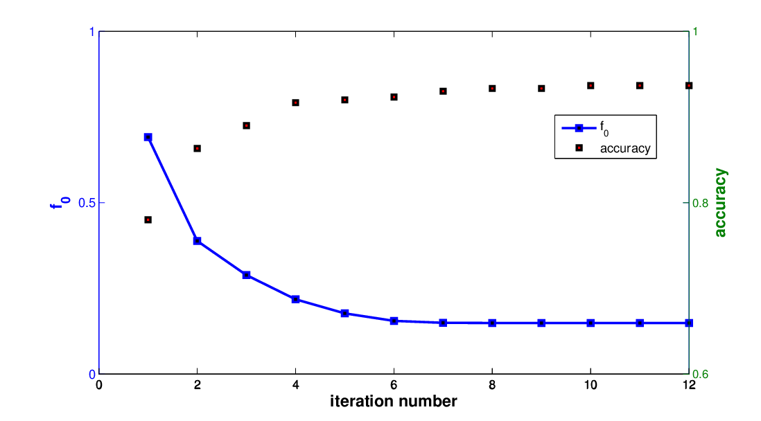
Our method can give the better solution for this problem by adapting the aggregation weights based on the observed data. When the results from a certain classifiers are unreliable, our method can remove the effect of this incorrect classifier on the overall classification accuracy by setting the corresponding aggregation weight to as close as to zero. We obtained the optimal aggregation weight vector by solving the optimization problem (10). Figure 3 shows the progress of primal-dual interior point method for this dataset. As mentioned in Section 3.1, the initial solution of the algorithm was set to a uniform weight vector, , in which our method produces the identical prediction to the loss-based decoding. As the algorithm converges, the classification accuracy evaluated using (the solution of each iteration) increases. The final solution of our method, , is given by
| (44) |
As we expected, the aggregation weight for , , becomes close to zero. With the optimal aggregation weight vector , the training classification accuracy is , which is much higher than that of loss-based decoding. The confusion matrix of our method is also given in Table 3.
| Predict | ||||
|---|---|---|---|---|
| class 1 | class 2 | class 3 | ||
| True | class 1 | 100 | 0 | 0 |
| class 2 | 0 | 92 | 8 | |
| class 3 | 0 | 10 | 90 | |
We further compared the performance of the loss-based decoding and our method, in the case where the number of classes is increased with the fixed number of training data. The data instances evenly sampled from number of 2-dimensional Gaussian distributions, the mean vectors of which are chosen as independent uniform random variables. We allowed the overlap of classes, thus the separation of classes might be harder as the number of classes is increased. For each trial samples were drawn from each Gaussian distribution, in which samples were used for training and 1000 samples for test. As the number of classes increase, the data points in each class became spares. With this synthetic data, we can examine the performance of our method for sparse dataset varying with the number of classes. We used the Liblinear (linear SVM) for the base binary classifier.
Figure 4 (b)-(d) represent the classification accuracy averaged over 20 independent runs, when the number of classes, , varies from 3 to 50 in the cases of APs, OVA and ECOC, respectively. Our method improves the classification accuracy of the loss-based decoding in the all cases. In addition, we can confirm that our method well works for the case where the number of data points in each class is relatively small compared to the number of classes.


(a) (c)


(c) (d)
5.3 Real-World Data
To compare the performance of each method on real-world problems, we used two cancer datasets and six UCI data sets [36]. The cancer data sets are acute lymphoblastic leukemia (ALL) [37] and global cancer map (GCM) [38], which were used to evaluate the performance of WMAP [16]. The detailed descriptions for the datasets are summarized in Table 4. All datasets were pre-processed such that all attributes are normalized to have unit variance, in order for attributes to reside in similar dynamic ranges. Especially, for two cancer datasets, we only selected a subset of genes as classification features: we chose genes as the input features by using a gene ranking based on the ratio of between group- to within group sum of squares. In addition to the cancer datasets, the input dimensionality of ’isolet’ dataset was reduced into 25 (equals to ) by Fisher linear discriminant analysis in order to reduce the computational complexity without loss of classification performance.
| samples | attributes | classes | |
|---|---|---|---|
| ALL | 248 | 12,558 | 6 |
| GCM | 198 | 16,063 | 14 |
| glass | 214 | 9 | 7 |
| segmentation | 2,310 | 19 | 7 |
| satimage | 6,435 | 36 | 7 |
| pendigits | 10,992 | 16 | 10 |
| isolet | 7,797 | 617 | 26 |
| letter | 20,000 | 16 | 26 |
In addition to classification accuracy, we evaluated mean square error (MSE) to examine the quality of class membership probability estimates obtained by the method. For a new test point , we usually have a corresponding true label, but not class membership probabilities. As in [10, 39], we can assume that the class membership probabilities are given by where is defined to be 1 if the label of is and 0 otherwise. Then, MSE is calculated as
| (45) |
where is the class membership probability estimated by the method. Note that MSE is also called Brier score [40], and the lower value the better performance.
For binary-decomposition methods, the base binary classifier was chosen according to the scale of dataset: LibSVM for the datasets {GCM, ALL}, and Liblinear [34] for other datasets. After learning of the binary classifiers, our method and WMAP were applied to learn the aggregation weights. Due to computational complexity, WMAP was applied to the small datasets, {GCM, ALL}. Otherwise, class membership probabilities for test dataset are calculated in the WMAP framework with the fixed aggregation weights. Each experiment was repeated 20 times by the random 10-fold cross-validation, in which the original data are randomly split into 10 subsets with the equal size, and then 1 subset is used for the validation data, and 9 subsets for the training data.
Table 5 summarizes the average accuracy for the different methods, M-SVM, LMR, loss-based decoding, GBTM, WMAP, and our method. The aggregation methods with APs encoding usually show the higher classification accuracy than two direct methods. This result is consistent with the comparison study in [5] which reported that APs-based decomposition methods generally show higher predictive accuracy than the direct methods for multiclass problems, such as M-SVM. In addition, our aggregation method shows superior performance than other methods across most of cases.
Table 6 shows the average MSE, which measures the quality of class membership probability estimate obtained by each method. At first we can check out that our method significantly improves the quality of class membership probability estimates of the loss-based decoding by tuning the aggregation weights. In addition, LMR generally shows high performance for most data sets, however, its performance does not exceed that of our method with APs encoding. We finally conclude that our aggregation method outperforms other methods, including the direct method, LMR, and two aggregation methods, GBTM and WMAP, in terms of the quality of class membership probability estimates. Note that, M-SVM is not considered in these cases due to its deterministic nature.
We also evaluated the performance of our method in terms of training time, reported in Table 7. As mentioned before, WMAP is prohibitive even for medium-scale problems: for GCM dataset, it averagely took 360.297 and 92.971 second to learn the aggregation weights in AP and OVA encodings, respectively. On the other hand, our method was terminated in seconds for most cases. Furthermore, our method has an additional computational advantage over the probabilistic decoding method based on (generalized) Bredely-Terry model, such as GBTM and WMAP, which involve additional optimizations to estimate the class membership probabilities for test data. In our method they are easily calculated by evaluating the softmax function (6) with the learnt aggregation weights. For example, we compared the test time of 3 probabilistic decoding methods, GBTM, WMAP and our method, on 6 UCI datasets. As shown in Table 8, our method is remarkably faster than other methods. As a results, we can confirm the superiority of our method in terms of computational efficiency as well as classification performance. Our method becomes more useful for large-scale multiclass problems which involve evaluating class membership probabilities for the data points.
| Dataset | M-SVM | LMR | Encoding | Loss-based | GBTM | WMAP | Our method |
|---|---|---|---|---|---|---|---|
| GCM | APs | 0.650(0.097) | 0.632(0.092) | 0.695(0.109) | 0.726(0.100) | ||
| 0.708 | 0.684 | OVA | 0.784(0.101) | 0.784(0.101) | 0.784(0.101) | 0.795(0.090) | |
| (0.110) | (0.109) | ECOC | 0.758(0.096) | 0.771(0.101) | 0.721(0.123) | 0.766(0.100) | |
| ALL | APs | 0.978(0.033) | 0.978(0.033) | 0.978(0.033) | 0.972(0.035) | ||
| 0.972 | 0.976 | OVA | 0.978(0.030) | 0.978(0.030) | 0.976(0.030) | 0.978(0.030) | |
| (0.037) | (0.027) | ECOC | 0.980(0.028) | 0.980(0.028) | 0.978(0.027) | 0.980(0.028) | |
| glass | APs | 0.564(0.102) | 0.576(0.094) | 0.564(0.099) | 0.602(0.098) | ||
| 0.638 | 0.631 | OVA | 0.600(0.098) | 0.600(0.098) | 0.598(0.102) | 0.610(0.108) | |
| (0.091) | (0.091) | ECOC | 0.629(0.109) | 0.629(0.109) | 0.626(0.111) | 0.640(0.088) | |
| segment | APs | 0.950(0.017) | 0.947(0.017) | 0.948(0.017) | 0.952(0.017) | ||
| 0.950 | 0.907 | OVA | 0.910(0.024) | 0.910(0.024) | 0.910(0.024) | 0.917(0.022) | |
| (0.020) | (0.019) | ECOC | 0.905(0.022) | 0.905(0.022) | 0.905(0.022) | 0.951(0.016) | |
| satimage | APs | 0.862(0.011) | 0.861(0.011) | 0.861(0.011) | 0.862(0.011) | ||
| 0.847 | 0.846 | OVA | 0.832(0.014) | 0.832(0.014) | 0.832(0.014) | 0.836(0.013) | |
| (0.011) | (0.015) | ECOC | 0.818(0.011) | 0.818(0.011) | 0.818(0.011) | 0.856(0.013) | |
| pendigits | APs | 0.979(0.005) | 0.977(0.006) | 0.977(0.006) | 0.979(0.005) | ||
| 0.956 | 0.934 | OVA | 0.931(0.007) | 0.931(0.007) | 0.931(0.007) | 0.934(0.008) | |
| (0.007) | (0.007) | ECOC | 0.918(0.025) | 0.928(0.009) | 0.928(0.009) | 0.958(0.008) | |
| isolet | APs | 0.974(0.005) | 0.973(0.005) | 0.973(0.005) | 0.978(0.004) | ||
| 0.976 | 0.960 | OVA | 0.972(0.005) | 0.972(0.005) | 0.972(0.005) | 0.972(0.005) | |
| (0.004) | (0.007) | ECOC | 0.959(0.008) | 0.965(0.006) | 0.965(0.006) | 0.969(0.006) | |
| letter | APs | 0.837(0.006) | 0.830(0.007) | 0.831(0.007) | 0.844(0.007) | ||
| 0.784 | 0.748 | OVA | 0.723(0.008) | 0.723(0.008) | 0.723(0.008) | 0.723(0.009) | |
| (0.009) | (0.010) | ECOC | 0.565(0.024) | 0.619(0.016) | 0.618(0.016) | 0.635(0.027) |
| Dataset | LMR | Encoding | Loss-based | GBTM | WMAP | Our method |
|---|---|---|---|---|---|---|
| GCM | 0.476(0.084) | APs | 0.923(0.001) | 0.569(0.068) | 0.553(0.066) | 0.417(0.148) |
| OVA | 0.917(0.002) | 0.322(0.082) | 0.347(0.079) | 0.287(0.125) | ||
| ECOC | 0.910(0.002) | 0.401(0.077) | 0.423(0.084) | 0.340(0.136) | ||
| ALL | 0.068(0.041) | APs | 0.784(0.002) | 0.067(0.048) | 0.060(0.047) | 0.039(0.050) |
| OVA | 0.739(0.005) | 0.042(0.041) | 0.048(0.046) | 0.038(0.049) | ||
| ECOC | 0.680(0.008) | 0.043(0.044) | 0.044(0.044) | 0.037(0.049) | ||
| glass | 0.516(0.116) | APs | 0.799(0.003) | 0.552(0.092) | 0.550(0.089) | 0.554(0.135) |
| OVA | 0.807(0.004) | 0.584(0.070) | 0.585(0.070) | 0.568(0.113) | ||
| ECOC | 0.791(0.006) | 0.568(0.068) | 0.569(0.067) | 0.538(0.116) | ||
| segment | 0.149(0.028) | APs | 0.819(0.000) | 0.107(0.018) | 0.132(0.017) | 0.075(0.023) |
| OVA | 0.798(0.002) | 0.149(0.022) | 0.153(0.022) | 0.112(0.023) | ||
| ECOC | 0.758(0.003) | 0.189(0.021) | 0.190(0.021) | 0.077(0.020) | ||
| satimage | 0.206(0.013) | APs | 0.783(0.000) | 0.192(0.013) | 0.196(0.012) | 0.187(0.015) |
| OVA | 0.764(0.001) | 0.242(0.012) | 0.244(0.012) | 0.224(0.015) | ||
| ECOC | 0.731(0.002) | 0.260(0.010) | 0.261(0.010) | 0.197(0.014) | ||
| pendigits | 0.110(0.009) | APs | 0.880(0.000) | 0.060(0.006) | 0.141(0.006) | 0.033(0.007) |
| OVA | 0.867(0.000) | 0.121(0.009) | 0.128(0.009) | 0.102(0.010) | ||
| ECOC | 0.860(0.002) | 0.162(0.015) | 0.178(0.014) | 0.065(0.011) | ||
| isolet | 0.085(0.007) | APs | 0.959(0.000) | 0.228(0.006) | 0.625(0.002) | 0.035(0.005) |
| OVA | 0.956(0.000) | 0.062(0.006) | 0.165(0.007) | 0.042(0.005) | ||
| ECOC | 0.945(0.001) | 0.114(0.008) | 0.171(0.008) | 0.048(0.007) | ||
| letter | 0.408(0.012) | APs | 0.959(0.000) | 0.339(0.006) | 0.663(0.002) | 0.232(0.007) |
| OVA | 0.959(0.000) | 0.495(0.006) | 0.592(0.005) | 0.396(0.009) | ||
| ECOC | 0.955(0.000) | 0.674(0.011) | 0.697(0.010) | 0.505(0.026) |
| Dataset | Encoding | iter | Time | Dataset | Encoding | iter | Time |
|---|---|---|---|---|---|---|---|
| GCM | APs | 18.5 | 0.114(0.013) | satimage | APs | 11.2 | 0.170(0.008) |
| OVA | 11.0 | 0.022(0.008) | OVA | 9.3 | 0.111(0.012) | ||
| ECOC | 12.6 | 0.053(0.007) | ECOC | 14.0 | 0.392(0.017) | ||
| ALL | APs | 11.0 | 0.021(0.007) | pendigits | APs | 13.8 | 1.350(0.044) |
| OVA | 9.0 | 0.015(0.007) | OVA | 9.0 | 0.313(0.013) | ||
| ECOC | 10.0 | 0.021(0.005) | ECOC | 14.9 | 1.544(0.046) | ||
| glass | APs | 13.7 | 0.032(0.010) | isolet | APs | 23.5 | 41.879(1.490) |
| OVA | 10.9 | 0.017(0.009) | OVA | 13.5 | 1.412(0.059) | ||
| ECOC | 15.0 | 0.043(0.008) | ECOC | 14.3 | 3.903(0.132) | ||
| segment | APs | 12.8 | 0.132(0.122) | letter | APs | 23.5 | 106.299(2.249) |
| OVA | 10.0 | 0.052(0.002) | OVA | 15.0 | 3.916(0.104) | ||
| ECOC | 15.9 | 0.355(0.028) | ECOC | 16.6 | 11.201(0.397) |
| Dataset | Encoding | GBTM | WMAP | Our method |
|---|---|---|---|---|
| APs | 0.178(0.026) | 0.174(0.006) | 0.000(0.000) | |
| glass | OVA | 0.258(0.024) | 0.163(0.005) | 0.000(0.000) |
| () | ECOC | 0.416(0.039) | 0.258(0.009) | 0.000(0.000) |
| APs | 6.286(0.083) | 2.316(0.034) | 0.001(0.000) | |
| segment | OVA | 5.234(0.170) | 2.264(0.052) | 0.001(0.000) |
| () | ECOC | 6.700(0.242) | 5.000(0.032) | 0.004(0.000) |
| APs | 15.331(0.134) | 6.398(0.114) | 0.001(0.000) | |
| satimage | OVA | 8.652(0.270) | 6.027(0.055) | 0.002(0.000) |
| () | ECOC | 11.776(0.582) | 9.247(0.032) | 0.004(0.000) |
| APs | 43.769(0.152) | 14.356(0.115) | 0.007(0.000) | |
| pendigits | OVA | 39.294(0.302) | 10.811(0.192) | 0.004(0.000) |
| () | ECOC | 45.466(0.957) | 28.057(0.873) | 0.008(0.001) |
| APs | 88.248(0.554) | 26.034(0.156) | 0.032(0.002) | |
| isolet | OVA | 68.645(0.210) | 9.614(0.305) | 0.019(0.002) |
| () | ECOC | 84.369(0.263) | 30.492(0.848) | 0.024(0.002) |
| APs | 214.264(2.927) | 94.640(1.006) | 0.133(0.176) | |
| letter | OVA | 167.560(6.766) | 24.462(0.358) | 0.051(0.005) |
| () | ECOC | 206.253(2.420) | 60.249(0.727) | 0.063(0.007) |
We additionally evaluated the classification performance of the aggregation methods with nonlinear binary classifiers. We used the LibSVM with a rbf kernel function for a base binary classifier, where the rbf-kernel width and the regularization parameter were determined by maximizing the classification accuracy of randomly chosen validation set on the 2-dimensional grid space (), and . Note that, the results on 2 cancer datasets (GCM and ALL) are not included in here because the performance on these datasets were considerable worse than using the linear kernel.
The average classification accuracy and MSE are shown in Table 9 and 10, respectively. As similar to the linear kernel case, our method showed the stable performance for the wide range of the value of . However, there was the slight degradation of performance of our method on the datasets {glass, satimage} due to overfitting, so we just increased the regularization parameter as for these datasets. We can see that all probabilistic decoding methods yield the similar classification performance for most cases. Although our method improves the results of the loss-based decoding in terms of MSE, its performance is not significantly better than that of GBTM and WMAP. The reason being is that optimal tuning of aggregation weights favors for good binary classifiers while de-emphasizing no good binary classifiers. When suitably-chosen nonlinear kernels are used, all binary classifiers are already good, so no much performance gain is shown even when optimal tuning of aggregation weights is made.
| Dataset | Encoding | Loss-based | GBTM | WMAP | Our method |
|---|---|---|---|---|---|
| glass () | APs | 0.681(0.090) | 0.681(0.088) | 0.695(0.070) | 0.683(0.094) |
| OVA | 0.676(0.090) | 0.676(0.090) | 0.676(0.090) | 0.681(0.085) | |
| ECOC | 0.683(0.104) | 0.686(0.105) | 0.683(0.096) | 0.695(0.093) | |
| segment | APs | 0.968(0.011) | 0.967(0.012) | 0.967(0.012) | 0.969(0.013) |
| OVA | 0.971(0.012) | 0.971(0.012) | 0.971(0.012) | 0.971(0.012) | |
| ECOC | 0.975(0.009) | 0.975(0.009) | 0.975(0.009) | 0.977(0.010) | |
| satimage () | APs | 0.924(0.009) | 0.924(0.009) | 0.924(0.009) | 0.924(0.010) |
| OVA | 0.925(0.009) | 0.925(0.009) | 0.925(0.009) | 0.925(0.010) | |
| ECOC | 0.927(0.010) | 0.927(0.010) | 0.927(0.010) | 0.927(0.010) | |
| pendigits | APs | 0.995(0.002) | 0.995(0.002) | 0.995(0.002) | 0.995(0.003) |
| OVA | 0.996(0.002) | 0.996(0.002) | 0.996(0.002) | 0.996(0.002) | |
| ECOC | 0.993(0.008) | 0.996(0.002) | 0.996(0.002) | 0.996(0.002) | |
| isolet | APs | 0.971(0.004) | 0.970(0.005) | 0.970(0.005) | 0.977(0.004) |
| OVA | 0.979(0.004) | 0.979(0.004) | 0.979(0.004) | 0.979(0.004) | |
| ECOC | 0.980(0.004) | 0.981(0.003) | 0.981(0.003) | 0.979(0.004) | |
| letter | APs | 0.973(0.004) | 0.973(0.004) | 0.972(0.003) | 0.974(0.003) |
| OVA | 0.978(0.004) | 0.978(0.004) | 0.978(0.004) | 0.977(0.004) | |
| ECOC | 0.976(0.005) | 0.978(0.003) | 0.978(0.003) | 0.978(0.004) |
| Dataset | Encoding | Loss-based | GBTM | WMAP | Our method |
|---|---|---|---|---|---|
| glass () | APs | 0.795(0.002) | 0.441(0.081) | 0.447(0.064) | 0.440(0.082) |
| OVA | 0.787(0.008) | 0.442(0.091) | 0.443(0.089) | 0.442(0.102) | |
| ECOC | 0.762(0.010) | 0.426(0.083) | 0.447(0.079) | 0.472(0.121) | |
| segment | APs | 0.818(0.000) | 0.059(0.015) | 0.075(0.014) | 0.047(0.018) |
| OVA | 0.783(0.001) | 0.043(0.015) | 0.044(0.014) | 0.046(0.017) | |
| ECOC | 0.718(0.002) | 0.037(0.012) | 0.037(0.012) | 0.039(0.017) | |
| satimage () | APs | 0.782(0.000) | 0.115(0.012) | 0.119(0.012) | 0.124(0.011) |
| OVA | 0.744(0.001) | 0.113(0.014) | 0.114(0.014) | 0.115(0.014) | |
| ECOC | 0.692(0.002) | 0.111(0.013) | 0.111(0.013) | 0.114(0.014) | |
| pendigits | APs | 0.881(0.000) | 0.018(0.003) | 0.089(0.003) | 0.008(0.004) |
| OVA | 0.860(0.000) | 0.006(0.003) | 0.009(0.003) | 0.006(0.003) | |
| ECOC | 0.853(0.003) | 0.007(0.003) | 0.011(0.003) | 0.006(0.003) | |
| isolet | APs | 0.959(0.000) | 0.115(0.007) | 0.563(0.002) | 0.036(0.005) |
| OVA | 0.956(0.000) | 0.035(0.005) | 0.114(0.005) | 0.034(0.005) | |
| ECOC | 0.944(0.001) | 0.032(0.004) | 0.067(0.005) | 0.035(0.006) | |
| letter | APs | 0.959(0.000) | 0.112(0.003) | 0.576(0.001) | 0.040(0.005) |
| OVA | 0.956(0.000) | 0.036(0.005) | 0.116(0.004) | 0.035(0.006) | |
| ECOC | 0.943(0.001) | 0.037(0.004) | 0.073(0.005) | 0.036(0.006) |
6 Conclusions
We have presented a method for optimally combining the results of binary classifiers into a final answer to multiclass problems. The softmax function was used to model the class membership probability, taking a conic combination of discrepancies induced by binary classifiers and returning a guess of class membership. The corresponding log-likelihood was a convex function in the form of log-sum-exp, leading to a convex formulation for optimal binary classifier aggregation. The primal-dual interior point method was adopted to solve the convex optimization problem.
Our method has several advantages over an existing optimal aggregation method, WMAP [16] which optimally combines binary class membership probability estimates to form a joint probability estimates for all classes, fitting the generalized Bradley-Terry model. In WMAP, both aggregation weights and class membership probabilities are treated as parameters to be estimated, so the computational complexity grows linearly with the number of training examples. In contrast, our method has a few strong points: (1) aggregation weights are the only parameters to be tuned (low complexity); (2) the convex formulation yields the global solution; (3) class membership probabilities for test data are easily evaluated without further optimizations. In addition, our method is available for any types of discrepancy measures, while the aggregation methods based on the (generalized) Bradley-Terry model always require that the binary classifier yields the probability estimates.
The (primal-dual) interior point method still suffers from computational burden in large scale problems. We may use a stochastic approximation of interior point methods [41] to improve the scalability. It is our future work to adopt more efficient optimization to speed up the computation and to improve the scalability, in our convex aggregation method.
7 Appendix
7.1 Derivations of gradient and Hessian of the objective function (10)
In this section, we include the gradient and Hessian of the objective function (10), which can be easily calculated based on the derivations of gradient and Hessian of the log-sum-exp function, described in Appendix in [22].
We first compute for and by (8). Then we define and for the th data point:
| (46) |
The objective function is given by
| (47) |
The gradient is computed as
The Hessian is obtained by
where .
7.2 Proof of Proposition 1
Proof. Let us define as the modified log-sum-exp function with , such that
We first show that the sequence of functions for uniformly converges to the multiclass hinge loss function . Then, we can easily prove that the sequence of functions also uniformly converges to . This proposition is an extension of the results in [42] which provide a connection between the hinge loss function and logistic loss function (that is a special case of the log-sum-exp function) in the case of binary problems.
For all , we are given the following inequalities for the log-sum-exp function [22]:
| (48) | |||||
Substituting into (48), one can easily see that
| (49) | |||||
It follows from this inequality that we have
| (50) | |||||
Thus, for any given , we can choose sufficiently large such that
Summing over all training data points, we obtain the inequality , which implies the uniform convergence of to .
7.3 Proof of Proposition 2
Proof. We first give the detailed explanations for some notations used in the proof. We can consider the margin of each example, , as a decision function for multiclass problems. For example, the data point is misclassified if and only if . Thus the empirical misclassification error can be defined by
| (51) |
where is the 0-1 loss function which equals 1 if the predicate is true, otherwise 0. In addition, due to the definition of the margin, we have
| (52) | |||||
where . Note that, since can be considered as feature mapping, as in kernel methods, the hypothesis set considered here is defined as a bounded linear function class, i.e., . In this work, we aim at finding an aggregation weight vector among the function class , which minimizes the expected misclassification error (generalization error), . However, a direct optimization involving the 0-1 loss is not an easy task because of its discrete nature. We instead consider a ramp loss , which is a continuous upper bound on 0-1 loss function:
Note that, is a clipped version of hinge loss [31]. Finally, we define the empirical Rademacher complexity [20] of a class of functions we are interested in. Let be a class of functions mapping from to and given samples , the empirical Rademacher complexity of the class is given by [20]
| (57) |
where are independent uniform random variables. Note that, the empirical Rademacher complexity is based on the training examples and thus is practically computable. In addition, it can be viewed as the correlation between a random binary noise and functions in the function class , in the supermum sense. In our case, the empirical Rademacher can be calculated based on Lemma 22 in [20]. Defining a new index , the empirical Rademacher complexity of the class is given by
| (58) | |||||
where Cauchy-Schwarz and Jensen’s inequalities are used to arrive at the second and the third inequalities respectively.
References
- [1] J. Weston and C. Watkins. Support vector machines for multi-class pattern recognition. In Proceedings of the Seventh European Symposium On Artificial Neural Networks, 1999.
- [2] K. Crammer and Y. Singer. On the algorithmic implementation of multiclass kernel-based vector machines. Journal of Machine Learning Research, 2:265–292, 2001.
- [3] A. C. Lorena, A. C. Carvalho, and J. M. Gama. A review on the combination of binary classifiers in multiclass problems. Artificial Intelligence Review, 30:19–37, 2008.
- [4] S. Knerr, L. Personnaz, and G. Dreyfus. Handwritten digit recognition by neural networks with single-layer training. IEEE Transactions on Neural Networks, 3:962–968, 1992.
- [5] C. W. Hsu and C. J. Lin. A comparison of methods for multiclass support vector machines. IEEE Transactions on Neural Networks, 13:415–425, 2002.
- [6] T. G. Dietterich and G. Bakiri. Solving multiclass learning problems via error-correcting output codes. Journal of Artificial Intelligence Research, 2:263–286, 1995.
- [7] E. L. Allwein, R. E. Schapire, and Y. Singer. Reducing multiclass to binary: A unifying approach for margin classifiers. Journal of Machine Learning Research, 1:113–141, 2000.
- [8] P. Domingos. MetaCost: A general method for making classifiers cost-sensitive. In Proceedings of the ACM SIGKDD Conference on Knowledge Discovery and Data Mining (KDD), pages 155–164, 1999.
- [9] D. D. Margineantu. Class probability estimation and cost-sensitive classification decisions. In Proceedings of the European Conference on Machine Learning (ECML), pages 270–281, 2002.
- [10] B. Zadrozny and C. Elkan. Obtaining calibrated probability estimates from decision trees and naive Bayesian classifiers. In Proceedings of the International Conference on Machine Learning (ICML), Williams Town, MA, 2001.
- [11] R. O. Duda, P. E. Hart, and D. G. Stork. Pattern Classification. John Wiely & Sons, 2001.
- [12] T. Hastie and R. Tibshirani. Classification by pairwise coupling. The Annals of Statistics, 26(2):451–471, 1998.
- [13] R. A. Bradley and M. E. Terry. Rank analysis of incomplete block designs: The method of paired comparisons. Biometrika, 39:324–345, 1952.
- [14] B. Zadrozny. Reducing multiclass to binary by coupling probability estimates. In Advances in Neural Information Processing Systems (NIPS), volume 14. MIT Press, 2002.
- [15] T. K. Huang, R. C. Weng, and C. J. Lin. Generalized Bradley-Terry models and multi-class probability estimates. Journal of Machine Learning Research, 7:85–115, 2006.
- [16] N. Yukinawa, S. Oba, K. Kato, and S. Ishii. Optimal aggregation of binary classifiers for multiclass cancer diagnosis using gene expression profiles. IEEE/ACM Transactions on Computational Biology and Bioinformatics, 6(2):333–343, 2009.
- [17] T. Takenouchi and S. Ishii. A multiclass classification method based on decoding of binary classifiers. Neural Computation, 21(7):2049–2081, 2009.
- [18] S. Park and S. Choi. Bayesian aggregation of binary classifiers. In Proceedings of the IEEE International Conference on Data Mining (ICDM), 2010.
- [19] S. Park and S. Choi. Geometric programming for classifier aggregation. In Proceedings of the IEEE International Conference on Acoustics, Speech, and Signal Processing (ICASSP), Prague, Czech Republic, 2011.
- [20] P. L. Bartlett and S. Mendelson. Rademacher and Gaussian complexities: Risk bounds and structural results. Journal of Machine Learning Research, 3:463–482, 2002.
- [21] J. C. Platt. Probabilistic outputs for support vector machines and comparisons to regularized likelihood methods. In Advances in Large Margin Classifiers, pages 61–74. MIT Press, 1999.
- [22] S. Boyd and L. Vandenberghe. Convex Optimization. Cambridge University Press, 2004.
- [23] S. Boyd, S. J. Kim, L. Vandenberghe, and A. Hassibi. A tutorial on geometric programming. Optimization and Engineering, 8(1):67–127, 2007.
- [24] Anthony V. Fiacco and Garth P. McCormick. Nonlinear Programming: Sequential Unconstrained Minimization Techniques. Jhon Wiley and Sons, 1968.
- [25] N. Karmarkar. A new polynomial-time algorithm for linear programming. Combinatorica, 4(4):373–395, December 1984.
- [26] J. Nocedal and S. J. Wright. Numerical Optimization. Springer, 1999.
- [27] K. M. Koh, S. J. Kim, and S. Boyd. An interior-point method for large-scale -regularized logistic regression. Journal of Machine Learning Research, 8:1519–1555, 2007.
- [28] T. Zhang and F. J. Oles. Text categorization based on regularized linear classification methods. Information Retrieval, 4:5–31, 2001.
- [29] D. P. Bertsekas. Nonlinear Programming. Athena Scientific, 1999.
- [30] S. Boyd and A. Mutapcic. Subgradient methods, 2007. Lecture Notes for Winter 2006-07, Stanford University.
- [31] R. Collobert, F. Sinz, J. Weston, and L. Bottou. Large scale transductive SVMs. Journal of Machine Learning Research, 7:1687–1712, 2006.
- [32] J. Friedman, T. Hestie, and R. Tibshirani. Regularization paths for generalized linear models via coordinate descent. Journal of Statistical Software, 33(1), 2010.
- [33] J. Nelder and W. M. Wedderburn. Generalized linear models. Journal of the Royal Statistical Society A, 135:370–384, 1972.
- [34] R. E. Fan, K. W. Chang, C. J. Hsieh, X. R. Wang, and C. J. Lin. LIBLINEAR: A library for large linear classification. Journal of Machine Learning Research, 9:1871–1874, 2008.
- [35] H. T. Lin, C. J. Lin, and R. C. Weng. A note on Platt’s probabilistic outputs for support vector machine. Machine Learning, 68(3):267–276, 2007.
- [36] A. Frank and A. Asuncion. UCI machine learning repository, 2010. URL http://archive.ics.uci.edu/ml.
- [37] E. J. Yeoh, M. E. Ross, S. A. Shurtleff, W. K. Williams, D. Patel, R. Mahfouz, F. G. Behm, S. C. Raimondi, M. V. Relling, A. Patel, C. Cheng, D. Campana, D. Wilkins, X. Zhou, J. Li, H. Liu, C. H. Pui, W. E. Evans, C. Naeve, L. Wong, and J. R. Downing. Classification, subtype discovery, and prediction of outcome in pediatric acute lymphoblastic leukemia by gene expression profiling. Cancer Cell, 1(2):133–143, 2002.
- [38] S. Ramaswamy, P. Tamayo, R. Rifkin, S. Mukherjee, C. H. Yeang, M. Angelo, C. Ladd, M. Reich, E. Latulippe, J. P. Mesirov, T. Poggio, W. Gerald, M. Loda, E. S. Lander, and T. R. Golub. Multiclass cancer diagnosis using tumor gene expression signatures. Proceedings of the National Academy of Sciences, USA, 98(26):15149–15154, 2001.
- [39] B. Zadrozny and C. Elkan. Transforming classifier scores into accurate multiclass probability estimates. In Proceedings of the ACM SIGKDD Conference on Knowledge Discovery and Data Mining (KDD), Edmonton, Canada, 2002.
- [40] G. W. Brier. Verification of forecasts expressed in terms of probability. Monthly Weather Review, 78:1–3, 1950.
- [41] P. Carbonetto, M. Schmidt, and N. de Freitas. An interior-point stochastic approximation method and an L1-regularized delta rule. In Advances in Neural Information Processing Systems (NIPS), volume 21. MIT Press, 2009.
- [42] J. Zhang, R. Jin, Y. Yang, and A. G. Hauptmann. Modified logistic regression: An approximation to SVM and its applications in large-scale text categorization. In Proceedings of the International Conference on Machine Learning (ICML), Washington, DC, 2003.