Inference on Self-Exciting Jumps in Prices and Volatility using High Frequency Measures Thanks: The authors would like to thank three anonymous referees and a co-editor for very detailed and constructive comments on an earlier draft of the paper. We also thank Yacine Aït-Sahalia, John Maheu, Eric Renault, George Tauchen, Victor Todorov and Herman van Dijk for very constructive comments at various stages in the development of the paper, plus the participants at the Society of Financial Econometrics Annual Conference, 2014, the International Association for Applied Econometrics Conference, 2014, and the Econometric Society Australasian Meetings, 2014. The research has been supported by Australian Research Council Discovery Grant DP150101728.
Abstract
Dynamic jumps in the price and volatility of an asset are modelled using a joint Hawkes process in conjunction with a bivariate jump diffusion. A state space representation is used to link observed returns, plus nonparametric measures of integrated volatility and price jumps, to the specified model components; with Bayesian inference conducted using a Markov chain Monte Carlo algorithm. An evaluation of marginal likelihoods for the proposed model relative to a large number of alternative models, including some that have featured in the literature, is provided. An extensive empirical investigation is undertaken using data on the S&P500 market index over the 1996 to 2014 period, with substantial support for dynamic jump intensities - including in terms of predictive accuracy - documented.
Keywords: Dynamic price and volatility jumps; Stochastic volatility; Hawkes process; Nonlinear state space model; Bayesian Markov chain Monte Carlo; Global financial crisis. JEL Classifications: C11, C58, G01.
1 Introduction
Planning for unexpected and large movements in asset prices is central to the management of financial risk. Key to this planning is the ability to distinguish extreme price changes arising from a persistent shift in the asset’s underlying volatility from idiosyncratic movements that occur due to random shocks in the market environment. Making this task more difficult is the fact that volatility itself exhibits discontinuous behaviour which, via the stylized occurrence of feedback from volatility to current and future returns (e.g. Bollerslev, Sizova and Tauchen, 2012), has the potential to cause seemingly discontinuous behaviour in the asset price. Moreover, it is unclear whether the apparent clustering behaviour of asset price jumps during times of market turbulence is evidence of dynamics in the jump intensity of either process (or both), or simply a result of the propagation through time of (independent) variance jumps due to persistence in the level of volatility.
Traditionally, parametric jump diffusion models have been used to capture the discontinuous behaviour in prices and, potentially, in their underlying volatility. Notable in this literature are the studies of Bates (2000) and Pan (2002), which propose models that characterize the intensity of a jump in price as proportional to the level of the underlying (diffusive) variance. In these models, the (price) jump intensity will be high in periods with high volatility and dependent over time as a consequence of the dynamic specification adopted for volatility itself. Duffie, Pan and Singleton (2000), on the other hand, introduce a model with both price and volatility jumps, and where the contemporaneous occurrence of the two types of jumps (i.e. the occurrence of ‘co-jumps’) is imposed. Under this specification, large fluctuations in price tend to occur in successive periods following a (contemporaneous) jump in price and volatility, again due to persistence in the volatility process. This impact is exacerbated by the fact that the expected price jump size is assumed to be conditionally (positively) dependent on the magnitude of the latent variance jump. Broadie, Chernov and Johannes (2007) also specify co-jumps, but impose independence between the sizes of the two different types of jump. Eraker, Johannes and Polson (2003), Chernov, Gallant, Ghysels and Tauchen (2003) and Eraker (2004) use more general specifications, in which both non-contemporaneous jumps and correlated jump sizes are accommodated, although insignificant correlation between the price and variance jump sizes is documented in all cases.
More recently, volatility and jump measures constructed from high frequency data have been used to investigate price and variance jumps, including the relationship between them. For example, the empirical findings of Todorov and Tauchen (2011) indicate the presence of jumps in volatility, whilst those of Jacod and Todorov (2010) provide evidence of both price and variance jumps, with a certain proportion of those jumps occurring simultaneously for the S&P500 market index. Jacod, Klüppelberg and Müller (2013) use high frequency data to explore the correlation between (imposed) co-jumps for several series, but fail to reject the null hypothesis of zero correlation in the majority of cases considered.
As highlighted clearly by Bandi and Reno (2016), however, the use (or otherwise) of option price data (and the associated risk premia specifications) in past analyses, plus the very nature of the volatility filter adopted (and data frequency exploited in the measurement of volatility), is likely to have had an impact on conclusions drawn regarding the joint evolution of a price and its variance, including discontinuities therein; with such considerations possibly underlying the inconclusive results recorded. We speculate that the rather restricted manner in which the dynamics in jumps have been modelled may also have played a role here.
With this background in mind, we propose a very general model for the joint evolution of price and volatility in which both processes are permitted to jump, co-jumps are possible (but not imposed), and both jump processes are allowed to be dynamic. To this end, we adopt a bivariate Hawkes process (Hawkes, 1971a,b) for the intensity of price and variance (accordingly volatility, defined as the square root of the variance) jumps, with both jump processes being (potentially) self-exciting as a consequence; that is, the intensity of each jump process is functionally dependent on the realized past increments of that process. We allow the variance jump intensity to depend on past price jumps, enabling extreme price movements to influence the occurrence of extreme movements in volatility. Possible leverage effects operating at the level of extreme price and volatility movements are also accommodated via the modeling of the differential impacts of negative and positive price jumps on the variance jump intensity.
A multivariate nonlinear state space framework, based on a discrete time representation of the proposed model, is specified. Three measures constructed from high frequency data, in addition to the daily return measure, are used to define the multiple measurement equations. The high frequency measures represent observed (price) jump occurrences and size, plus (logarithmic) bipower variation. A Bayesian analysis of the model is undertaken using a Markov chain Monte Carlo (MCMC) algorithm that accommodates the numerous sources of non-linearity in the state space model, and that samples the latent diffusion variances efficiently in blocks. The conditionally deterministic (Hawkes) specification for the jump intensities is computationally convenient, with the posterior distribution of both intensities at any time point - including future time points - able to be estimated from the MCMC draws of the parameters and latent variables to which the intensities are functionally related.
Application of the methodology to data on the S&P500 index for the period January 1996 to June 2014 is documented in detail. The empirical analysis includes the calculation of marginal likelihoods for evaluating the proposed specification against multiple alternatives, most of which are nested within our general state space model and many of which share features with (or, indeed, coincide with) models that have featured prominently in the literature. Predictive distributions are also computed, for the purpose of out-of-sample assessments. The comparative models include those in which the price and variance jump intensities are dynamic as a consequence of a functional dependence (either linear or non-linear) on the level of volatility. Two realized generalized autoregressive conditional heteroscedasticity (RGARCH) specifications of Hansen, Huang and Shek (2012) are also entertained, as alternatives to the state space form.
As in Bandi and Reno (2016) spot price data only is used to analyse all models, with the results unaffected as a consequence by the nature of - and potential dynamics in - volatility and jump risk premia (see Bollerslev, Gibson and Zhou, 2011, and Maneesoonthorn, Martin, Forbes and Grose, 2012, for analyses in which such specifications do feature). However, and in contrast with Bandi and Reno, data measured at the daily frequency (including that which aggregates to the daily level over intraday observations) underpins the analysis. In common with the large part of the relevant literature (Bollerslev, Kretschmer, Pigorsch and Tauchen, 2009, and Liu, Patton and Sheppard, 2015, amongst many others) we also choose to construct all measures using within-day observations only, thereby avoiding the need to model close-to-open movements in the index (as in, for example, Ahoniemi, Fuertes and Olmo, 2015, and Andersen, Bollerslev and Huang, 2011) and any specific dynamic movements therein. (See Hansen and Lunde, 2005, and Takahashi, Omori and Watanabe, 2009, for earlier discussions on the role played by non-trading periods in the construction of high frequency measures).
The remainder of the paper is organized as follows. Section 2 describes our proposed asset price model and its main properties. The continuous time representation is presented first, followed by the discrete time state space structure adopted for inference. Details are given of the high frequency measures of volatility and price jumps that are used to supplement daily returns in defining the state space model. The Bayesian inferential approach is then outlined in Section 3, including the way in which the alternative specifications are to be assessed, relative to the most general model, both in terms of marginal likelihoods and cumulative log scores. Results from the extensive empirical analysis of the S&P500 index are presented and discussed in Section 4. The benefits of allowing for a very flexible dynamic specification for price and variance jumps are confirmed by both the within-sample and predictive assessments, with the bivariate Hawkes specification given strong support by the data, relative to other more restrictive models. The empirical results also indicate that two jump intensity processes differ in terms of their time series behaviour. Most notably, the variance jump intensity is much more closely aligned with market conditions, exhibiting its most dramatic increase at the peak of the global financial crisis in late 2008. Section 5 provides some conclusions. Certain technical results, including algorithmic and prior specification details, are included in appendices to the paper.
2 An asset price process with stochastic volatility and self-exciting jumps
2.1 The continuous time representation
Let be the natural log of the asset price, at time , whose evolution over time is described by the following bivariate jump diffusion process,
| (1) | ||||
| (2) |
with and denoting standard Brownian motion processes, and , for . Without the discontinuous sample paths and this form of asset pricing process replicates that of the Heston (1993) square root stochastic volatility model, where the parameter restriction ensures the positivity of the variance process, denoted by for . The drift component of (1) contains the additional component , allowing for a volatility feedback effect (that is, the impact of volatility on future returns) to be captured, while in (2) captures the leverage effect (that is, the impact of (negative) returns on future volatility). (See Bollerslev, Livitnova and Tauchen, 2006, who also propose a model that separates volatility feedback from leverage effects.) The , are dependent random jump processes that permit occasional jumps in either or , or both, and have random sizes and , respectively.
A novel contribution of this paper is the specification of a bivariate Hawkes process for the point processes, , which feeds into the bivariate jump process, Specifically, we assume that
| (3) | ||||
| (4) |
and that
| (5) | ||||
| (6) |
where denotes the occurrence of a negative price jump, corresponding to a value of one for the indicator function Due to the inclusion of the terms and in (6), the process defined by (5) is not only ‘self-exciting’, but is also excited by a concurrent price jump. The additional threshold component, , allows a contemporaneous negative price jump to have a differential impact (as compared with a positive price jump) on , thereby serving as an additional channel for leverage, over and above the non-zero correlation between the Brownian motion increments, and The parameters , are the steady state levels of the respective intensity processes to which the intensities revert once the impact of excitation dissipates. See Hawkes (1971a,b) for seminal discussions regarding self-exciting point processes, and Aït-Sahalia, Cacho-Diaz and Laeven (2015) for the introduction of the Hawkes process into asset pricing models.
Our proposed specification can be viewed as a natural extension of the various models in the literature that accommodate both stochastic volatility and jumps. Most notably we relax the strict assumption of contemporaneous price and volatility jumps as imposed, for example, by Duffie et al. (2000), Broadie et al. (2007) and Bandi and Reno (2016). Instead, price and volatility jumps are governed by separate, but dependent, dynamic random processes, such that the two types of jumps may or may not coincide. As detailed below, the probability of co-jumps can be readily computed from the MCMC output, as can the posterior distributions for the magnitude of both types of jumps (whether coincident or not). The specification can also be viewed as an extension of the stochastic volatility model of Aït-Sahalia et al. (2015), in which a Hawkes process is used to characterize multivariate price jump occurrences, but with variance jumps absent from the model. Similarly, it extends the model proposed by Fulop et al. (2014), in which price jump intensity (only) is characterized by a Hawkes process, along with the restrictive assumption that variance jumps occur contemporaneously with negative price jumps.
2.2 A discrete time model for returns
In common with the literature, we undertake inference in the context of a discrete time state space representation of the continuous time model for the asset price, applying an Euler discretization to (1) through (6) with (equivalent to one trading day). Given the complexity of the proposed model, and the multiple features on which we wish to draw inference, we supplement the daily return measure, defined as
where denotes the logarithm of the asset price at the end of day , with three additional measures computed from high frequency (intraday) returns. For expositional clarity we begin, in this section, by focusing on the measurement equation for the return only, describing in detail the latent components that feature therein. In Section 2.3 we then introduce the high frequency quantities that are used to define the three additional measurement equations, making clear the assumed link between observed and latent quantities. In Section 2.4, we collect all components of the model together, introducing appropriate labelling to facilitate subsequent referencing.
We begin then with the measurement equation based on the daily return,
| (7) |
where the variation in is driven by the latent diffusive volatility process and the latent price jump component . The (daily) evolution of diffusive volatility is given by
| (8) |
with the leverage parameter, , taken into account explicitly. The error components and , in (7) and (8), respectively, are defined as marginally serially independent sequences, with for each .
The latent occurrences of price and volatility jumps on day are expressed as
| (9) | ||||
| (10) |
with , and where the probabilities of success are driven (respectively) by the discretized intensity processes,
| (11) | ||||
| (12) |
The discretized jump intensities, and , possess a conditionally deterministic structure that is analogous to that of a generalized autoregressive conditional heteroskedastic (GARCH) model for latent volatility, with the lagged jump occurrences playing a similar role to the lagged (squared) returns in a GARCH model (Bollerslev, 1986). Assuming stationarity, the unconditional mean for the price intensity process is determined by taking expectations through (11) as follows,
and solving for the common value as
| (13) |
Similarly, the unconditional mean of the variance jump intensity process in (12) is given by with
resulting in
| (14) |
where denotes the probability that the price jump is negative. By substituting into equation (14) the expression for in (13), may be re-expressed as the following function of static parameters,
To ensure that and , the restrictions , , and are required. Note that the parameters used in (7)-(12) are the discrete time versions of the corresponding parameters in the continuous time model (1)-(6), but with the same symbols used for notational simplicity.
The size of the latent volatility jump is assumed to be exponentially distributed,
with only positive volatility jumps allowed as a consequence. The latent price jump size, on the other hand, is assumed to be composed of two parts: magnitude and sign, ensuring adequate characterisation of the empirically observed bimodal feature of the measured price jump distribution (see further discussion of this point in Section 4). Specifically, we assume,
where, with as defined earlier, the random variable,
determines the sign of the price jump, and
| (15) |
determines the logarithmic magnitude, with a mean value that is proportional to the underlying volatility
The factors that drive the return in (7) can be interpreted as follows. Consistent with the empirical finance literature (see, for example, Engle and Ng, 1993, Maheu and McCurdy, 2004, and Malik, 2011), the diffusive price shock, and the price jump occurrence, are collectively viewed as ‘news’. Regular modest movements in price, as driven by , are assumed to result from typical daily information flows, with (all else equal) the typical direction of the impact of on the variance of the subsequent period, , captured by the sign of . The occurrence of a price jump however, indicated by , can be viewed as a sizably larger than expected shock that may signal a shift in market conditions, with the probability of subsequent price and/or variance jumps adjusted accordingly, through the model adopted here for the jump intensities. That is, the process can be viewed as being potentially self-exciting: provoking an increase in the future intensity (and thus occurrence) of price jumps (via (11)), as well as provoking (or exciting) an increase in the future intensity of variance jumps (via (12)). The threshold parameter in (12) allows for a possible additional impact of a negative price jump on the variance jump intensity (and, hence, the level of volatility), providing an additional channel for leverage, as noted above.
From the form of (7) and (8), the implications for returns of the occurrence of the two types of jumps are clear. From (7), the direct impact of a given price jump at time , , is felt only at time . However, clusters of price jumps and, hence, successive extreme values in returns, can occur via the dynamic intensity process in (11) that drives subsequent realizations of . The impact of a given (positive) variance jump at time will carry forward through time via the persistence of the process, as governed by . That is, if the return variance jumps in any period, it will tend to remain higher in subsequent periods and, thus, be expected to cause larger movements in successive prices than would otherwise have occurred. In addition, any clustering of variance jumps, driven by the dynamic intensity process in (12), would simply cause an exaggeration of the resultant clustering of extreme returns. Arguably, clusters of jumps in the latent variance would typically be associated with sustained market instability, with the variance jump intensity expected to increase and remain high during periods of heightened market stress. We return to this point in Section 4.
2.3 Incorporating high frequency measurements of volatility and price jumps
In the spirit of Barndorff-Nielsen and Shephard (2002), Creal (2008), Takahashi et al. (2009), Dobrev and Szerszen (2010), Jacquier and Miller (2010), Hansen et al. (2012), Maneesoonthorn et al. (2012), and Koopman and Scharth (2013), amongst others, we exploit high-frequency data to supplement the measurement equation in (7) with additional equations based on nonparametric measures of return variation: both its diffusive and jump components. As is now standard knowledge, realized variance, defined by
| (16) |
where denotes the observed return the over the horizon to , and there being such returns, is a consistent estimator of quadratic variation under the assumption of no microstructure noise. (See, for example, Barndorff-Nielsen and Shephard, 2002 and Andersen, Bollerslev, Diebold and Labys, 2003). Quadratic variation, , in turn, captures the variation in the return over the horizon to due to both the stochastic volatility and price jump components, with where denotes the integrated variance, and denotes the price jump variation. With bipower variation,
| (17) |
being a consistent measure of (again, in the absence of microstructure noise), the discrepancy between in (16) and in (17) serves as a measure of price jump variation, and has, as a consequence, formed the basis of various tests of the significance of jump variation on any particular day; see, for example, Barnorff-Nielsen and Shephard (2004, 2006) and Huang and Tauchen (2005).
Three measurement equations that exploit the information content in and are constructed as follows. First we define a measure that indicates the occurrence or otherwise of a price jump on day ,
| (18) |
where
| (19) |
and is the critical value in a standard normal distribution, associated with significance level The term in the denominator of (19) denotes an estimate of the integrated quarticity, with having a limiting standard normal distribution under the assumption of no jumps, as a result of the particular standardization used in its definition; see Huang and Tauchen (2005) for details. The indicator function in (18) is then viewed as a noisy measure of the latent price jump occurrence in (9). That is, we specify the measurement equation,
with constant probabilities and to be estimated from the data.
Second, we assume that the latent (logarithmic) price jump size in (15) is measured with error by
| (20) |
where
| (21) |
by specifying the measurement equation,
with 11 1 Note that when , which, from (21), occurs when , we do not view the data as providing any information about price jump size, and with being undefined in this case.
Third, as a direct measure of integrated volatility, is assumed to bring noisy information about the diffusive volatility process, including any jumps in such a process. Hence (and utilizing in logarithmic form in order to better justify the assumption of a Gaussian measurement error), we specify a final measurement equation as
where , where is a discretization of and the estimation of and as free parameters allows for to be a biased measure of
2.4 The full discrete time state space model
For expositional clarity, we collect together here all components of the model, beginning with the four measurement equations:
| Daily return | (22) | |||
| Price jump indicator | ||||
| Log price jump size | (25) | |||
| Log bipower variation | (26) |
The stochastic state processes comprise:
| Latent volatility | ||||
| (27) | ||||
| Latent price jump occurrence | (28) | |||
| Latent volatility jump occurence | (29) | |||
| Latent price jump size | (30) | |||
| Latent volatility jump size | (31) |
where the specification of the latent price jump in (30) is given by the product of two random components, with one relating to the jump direction:
and the other relating to the log price jump magnitude:
Finally, the two conditionally deterministic states are given by:
| Price jump intensity | (32) | |||
| Volatility jump intensity | ||||
| (33) |
All subsequent referencing of the model makes use of the equation numbering in this section.
3 Bayesian inference
3.1 Overview
For notational convenience, we collectively denote, at time point , the measurement vector as and the latent state vector as , with the static parameters also collectively denoted by the vector
| (34) |
In addition, we denote time-indexed variables generically as, for example, for , where is empty. The joint posterior density associated with the full model in (22)-(33), denoted subsequently by , satisfies
| (35) |
Note that this joint posterior assumes that and . In the specification of the prior in (35) we use a combination of noninformative and weakly informative distributions for the various elements of . Other than exploiting the natural groupings of parameters that arise from the regression structures embedded within the model, we adopt a priori independence for the individual parameters. The detailed specifications of each component of are documented in Appendix A.
Given the complexity of the state space representation, and the high dimension of the set of unknowns, the posterior indicated by (35) is not available in closed form. Hence, a hybrid of the Gibbs and Metropolis-Hastings (MH) MCMC algorithms is developed to obtain draws of the static parameters and latent variables of interest from the joint posterior distribution, with inference - including the construction of posterior predictive distributions - conducted using those draws. Details of this algorithm, including a reference made to Maneesoonthorn et al. (2012) for a full description of the multi-move algorithm adopted for sampling the variance state vector, , are given in Appendix B.1.
3.2 Models of interest and their marginal likelihoods
As has been highlighted, a novel aspect of our specification is that it allows for dynamic behaviour in both price and variance jumps, as well as various types of dependencies between those extreme movements. It is of interest then to explore whether or not this rich dynamic structure is warranted empirically, through an investigation of various simpler specifications.
To this end, we consider several competing models, summarized in Table 1, most of which are nested in the full model specification in (22) to (33), and all of which are to be evaluated empirically in Section 4. First (and with reference to the labelling of models in the left-most column of the table), a model without a threshold component (that is, without the differential impact on variance jump intensity due to the occurrence of negative price jumps) is specified as . Next, model specifies that the occurrence of price jumps has no impact at all on the variance jump intensity, via the removal of both price jump feedback terms from . That price and variance jumps occur contemporaneously, or that the variance does not jump at all, each correspond to further restrictions specified in and , respectively. Note that shares some features with the model proposed by Aït-Sahalia et al. (2015), albeit in a single asset setting here. In models to , and as an alternative to the use of the bivariate Hawkes process, the jump intensities are specified as various functions (both linear and non-linear) of the latent variance, with sharing some common features with the models adopted in Bates (1996), Pan (2002), and Eraker (2004). In we then specify constant jump intensities, yielding the stochastic volatility with the independent jumps (SVIJ) model of Duffie et al. (2000), whilst in we consider the absence of both price and variance jumps, with the resultant latent process thereby coinciding with that of the conventional Heston (1993) square root model.
Finally, we provide an alternative to the state space form, entertaining the conditionally deterministic RGARCH(1,1) model of Hansen et al. (2012), specified as
| (36) | ||||
| (37) |
where and , with and defining the evolution of the deterministic variance and the bipower variation, respectively. In our comparison, we entertain both the linear and the log-linear specifications of RGARCH, denoted by and respectively, with details given in Table 1. These two models are, of course, not nested in the general state space framework, and details of the separate MCMC algorithm used to estimate the relevant posterior densities are provided in Appendix B.2.
To examine the relative merits of these twelve models of interest, computation of their corresponding marginal likelihood values,
| (38) |
for and is required. Under the assumption that each of the models is a priori equally likely, the posterior odds ratio for the full state space model relative to any restricted model is equivalent to the Bayes factor , given in turn by
| (39) |
Given Bayes factors and , the Bayes factor for model relative to model is obtained simply as
Note that both and the first eight comparator models are estimated using the full set of measurements. However, models and do not exploit observed price jump information, given the absence of any jumps specified in either the price or latent volatility component, with all three models estimated using only observations on and as a consequence. This gives us two possibilities regarding the computation of the Bayes factors for these models. Firstly, we can compute the marginal likelihoods using only observations on and and compare the three marginal likelihoods to each other only. Alternatively, we can augment these marginal likelihoods with an additional factor that caters for the price jump measurements, computed using priors that are consistent with the imposition of no jumps within the models. These latter (expanded) quantities can then be used in a comparison, via the computation of Bayes factors, with the other eight specifications. We record both forms of results in Section 4.
| Model | Restrictions | Description |
|---|---|---|
| None | Full state space model: (22) to (33) | |
| Full model without threshold component | ||
| Full model without price jump feedback | ||
| Full model with contemporaneous jumps | ||
| Hawkes model without volatility jumps | ||
| State dependent jump intensity: linear | ||
| State dependent jump intensity: quadratic | ||
| State dependent jump intensity: logistic | ||
| Constant jump intensity | ||
| Stochastic volatility model without jumps | ||
| RGARCH model: linear | ||
| RGARCH model: log-linear |
The marginal likelihood for model in (38) is challenging to compute, in particular for the state space specifications, which require the calculation of an integral over a very large dimension due to the number of latent variables present. As per Chib (1995) and Chib and Jeliazkov (2001), we estimate the marginal likelihood of each model using the output of a series of auxiliary MCMC algorithms, in addition to the full MCMC algorithm associated with estimation of the given model. Specific details of this computation are provided in Appendix C. A brief explanation of the computation of the marginal likelihoods for the three restricted models ( and ) is also provided in this appendix.
3.3 Predictive performance
With reference to the joint measurement vector at time , and model , and , the one-step-ahead predictive distribution as based on information up to time is given by
| (40) | ||||
where denotes the vector of static parameters associated with model , and represents the full set of latent variables that feature therein. For the RGARCH models, of course, is an empty set, so that the integration occurs over only. As is well known (see, for example, Geweke, 2001) the log marginal likelihood for any model , and , computed over the entire sample period 1 to , may be expressed as the sum of log marginal predictive densities, each associated with , and evaluated ex-post at the corresponding observed values:
| (41) |
It follows that the Bayes factor in (39) may actually be interpreted as providing a measure of predictive accuracy for model , relative to that of model , over the entire sample period. Importantly, the component predictive distributions in (41) do not rely upon any unknown parameters, and reflect the evaluation of predictions made without reference to any future information.
What is absent from the computation of the full sample Bayes factor, however, is any information on the change over the sample period in the predictive performance relative to . To better capture this dynamic predictive behaviour, we compute the cumulative difference in log score (CLS) over an evaluation (sub-) period of trading days, according to
| (42) |
for . An increase in the value of , relative to indicates an improvement in the performance of the reference model, relative to , in terms of predicting all four elements of , with a persistent positive level in indicating sustained predictive superiority of relative to , over that period. Note that for the early values in this set of sequential calculations to be reliable, an initial sample consisting of observations, , is used to initialise the computation. (See also Geweke and Amisano, 2010). Estimation of (40) and, subsequently, computation of (42), occurs via a combination of MCMC and particle filtering algorithms, with further details provided in Section 4.4.
To complement the CLS results as they pertain to the joint measurement vector , in Section 4.4 we also report predictive performance as it relates to certain individual sub-vectors of . Denote any sub-vector of by . Then we define the marginal CLS for as
| (43) |
again for . Specifically, we report predictive results for the return, where and the log bipower variation, where , as well as for the bi-variate subvector containing the price jump indicator and size components, where
| (44) |
Computation of the terms comprising the marginal CLS in (43) for a given requires a relatively small modification of the methodology used to compute the joint quantities in (40) and (42), with details provided in Section 4.4. Isolation of the predictives for individual elements of also enables us to directly compare the predictive performance of models and with , in terms of the accuracy with which these two models forecast future values of and specifically. In the case of and , given the absence of stochastic latent variables, computation of the predictive quantities using the MCMC draws from the joint posterior is standard, without there being any need for additional filtering steps.
4 Empirical application
4.1 Data description and preliminary analysis
For the empirical analysis documented below, 4598 observations on the open-to-close logarithmic S&P500 return (), price jump indicator (), logarithmic price jump size and logarithmic bipower variation () were analyzed, over the period January 3, 1996 to June 23, 2014. The index data has been supplied by the Securities Industries Research Centre of Asia Pacific (SIRCA) on behalf of Reuters, with the raw intraday index data having been cleaned using methods similar to those of Brownlees and Gallo (2006). The measures constructed from high-frequency data are based on fixed five minute sampling, with a ‘nearest price’ method (Andersen, Bollerslev and Diebold, 2007) applied to construct the relevant returns five minutes apart, and only index values recorded within the New York Stock Exchange market trading hours. The numerical results reported in this empirical section have been produced using a combination of the JAVA and MATLAB programming languages. Marginal posterior point and interval summaries for the static parameters are reported in Section 4.2 for the full model only, with results pertaining to all competing models recorded in Table 1 provided in the on-line supplementary appendix.

In Figure 1 we provide a graphical representation of two of the four measures, and (the latter in both raw and logarithmic form) for the entire sample period, recorded in annualized form. As is evident in both panels of Figure 1, and as is completely expected in this setting, volatility clustering is a marked feature. The most extreme variation in returns, along with the occurrence of values of unprecedented magnitude, is observed towards the end of 2008. The large jumps observed periodically in , in addition to the jumps in evidence in the return series itself, plus the tendency for both types of jumps to cluster, all provide motivation for the specification of a dynamic model for both price and volatility jumps.
In Panel A of Figure 2 we plot the time series of the signed jump size measure , with and as defined in (18) and (21) respectively, with the data indicating that price jump intensity is 10.64% on average.22 2 With reference to (18), is defined using a significance level of , as recommended by Tauchen and Zhou (2011). Values of the combined measure are indicated on the left-hand-side axis.33 3 We reiterate that the sign of the price jump is modelled as a latent process only (in (30)), and is estimated along with all other unknowns in the model. We do not assume that the sign of the price jump coincides exactly with the sign of the return on that day. We represent the direction of the price jump by the sign of the return for the purpose of this preliminary diagnostic exercise only. Distinct variation in the observed price jump size over the sample period, including clusterings of both small and large jumps, is evident, with there being no particular tendency for negative price jumps (as identified here simply by the occurrence of a negative return) to predominate over this extended period. Clusters of large jumps appear intermittently over the sample period; however, the clusters that are largest in magnitude occur during three of the most volatile market periods: late 2001 and throughout 2002 following the September 11 terrorist attacks; the global financial crisis period in 2008 and 2009; and the culmination of the period of Euro-zone debt crises, in 2011. The logarithmic measure of price jump magnitude, , (as defined in (20)), is also included in Panel A, with values indicated on the right-hand-side axis. The fluctuations in this variable reflect (via the logarithmic transformation of ) the changes in the observed price jump size, with changes that are large in magnitude producing large positive values for , and very small magnitude changes in yielding negative values for
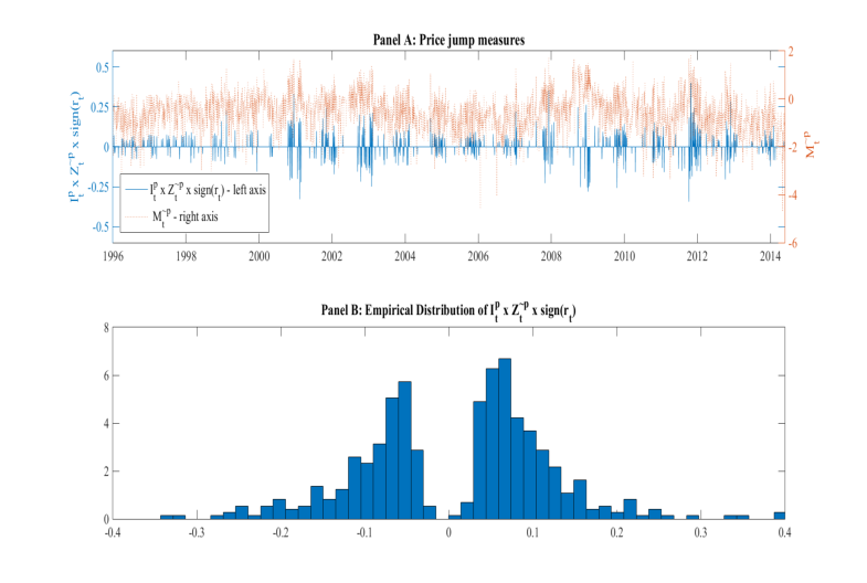
Panel B of Figure 2 depicts the histogram of the signed jump size measure, . As is consistent with the time series plot in Panel A, there is no evidence of negative jumps occurring more frequently than positive jumps throughout the entire sample period. In addition, the empirical distribution is seen to be bimodal, with the very small probability mass in the neighbourhood of zero reflecting the fact that, conditional on a significant jump occurring, the size of that jump is, necessarily, bounded away from zero. This bimodal feature of the observed price jump magnitude does not appear to have been recognized in the literature, with a Gaussian distribution typically adopted for the latent variable . (See Eraker et al., 2003, and Tauchen and Zhou, 2011, for example). In contrast, our approach adopts as a (noisy) measure of the latent (log) jump size, , only when is non-zero, and thereby both accommodates this observed bimodality and avoids a Gaussian assumption for itself.44 4 We are grateful to an anonymous referee who highlighted the need to accommodate this non-Gaussianity in our modelling of the price jump size.
4.2 The implied Hawkes dynamics
To illustrate the dynamic structure implied by our full state space model , we provide here posterior summary information relating to the static parameters, including the parameters of the two jump intensity processes, corresponding to the full sample period. Reported in Table 2 are the marginal posterior means (MPMs) and 95% highest posterior density (HPD) intervals for the static parameters in (34), calculated from 30,000 MCMC draws (following a 30,000 draw burn-in period) of which every 5th draw is saved. Inefficiency factors computed from the retained posterior draws are also reported in the table, estimated as the ratio of the variance of the sample mean of a set of MCMC draws of a given unknown, to the variance of the sample mean from a hypothetical independent sample. All parameter summaries are reported in annualized terms where appropriate. For example, the magnitude of the parameter accords with an annualized variance quantity, whilst reflects the daily persistence in that annualized variance. We also record point and interval estimates of the probability of simultaneous and sequential price and volatility jumps, in the last two lines in the table.
The inefficiency factors reported in Table 2 (for the static parameters) range from 1 to 150, with certain parameters associated with the variance jump intensity producing the highest values. The inefficiency factors for all latent variables, computed at selected time points (and not reported here), range from 3 to 5. The acceptance rates for all parameters drawn using MH schemes range from 15-30%, with the acceptance rate for drawing (in blocks) - computed as the proportion of times that at least one block of is updated over the entire MCMC chain - being approximately 99%. The convergence of the MCMC chains for all unknowns is also confirmed via inspection of graphical CUSUM plots (Yu and Mykland, 1998), and using the convergence diagnostics prescribed by Heidelberger and Welch (1983) and Geweke (1992).
| Parameter | MPM | 95% HPD interval | Inefficiency Factor |
|---|---|---|---|
| 0.199 | (0.139,0.256) | 1.59 | |
| -8.628 | (-9.955,-5.679) | 1.10 | |
| -0.357 | (-0.421,-0.289) | 6.54 | |
| -0.419 | (-0.435,-0.403) | 6.43 | |
| 10.955 | (9.967,11.970) | 22.83 | |
| 0.207 | (0.187,0.226) | 13.84 | |
| 0.382 | (0.297,0.470) | 12.76 | |
| 8.99 | (2.39,3.33) | 1.82 | |
| 0.814 | (0.633,0.956) | 17.17 | |
| 0.183 | (0.162,0.203) | 13.47 | |
| 0.970 | (0.796,1.142) | 116.60 | |
| 1.290 | (1.255,1.325) | 81.16 | |
| 0.436 | (0.423,0.450) | 5.75 | |
| 0.116 | (0.092,0.167) | 45.97 | |
| 8.19 | (7.41,9.11) | 15.79 | |
| 0.016 | (0.014,0.017) | 19.25 | |
| 9.66 | (8.21,0.012) | 48.48 | |
| 0.132 | (0.108,0.170) | 14.96 | |
| 0.097 | (0.072,0.127) | 9.18 | |
| 0.062 | (0.047,0.079) | 12.12 | |
| 0.121 | (0.082,0.158) | 41.23 | |
| 0.035 | (0.024,0.050) | 149.68 | |
| 0.030 | (0.021,0.043) | 134.58 | |
| 5.51 | (1.33,2.00) | 1.77 | |
| 1.14 | (3.11,3.84) | 2.34 | |
| 0.097 | (0.059,0.139) | 20.35 | |
| 0.107 | (0.066,0.149) | 30.12 |
The parameters associated with the two jump intensity processes are, of course, our primary interest. The dynamic price jump intensity, , possesses a reasonably strong degree of persistence, as indicated by the relatively low MPM of , and an HPD interval for that is well above zero, consistent with the presence of self-excitation. The magnitudes of and reported here, once annualized, are consistent with the parameters reported by Aït-Sahalia et al. (2015), who (as noted earlier) propose a Hawkes process for price jumps, but omit variance jumps in their stochastic volatility specification.
The MPM of the long-run variance jump intensity, , is relatively high compared with previously reported (comparable) quantities (Eraker et al., 2003, Eraker, 2004 and Broadie et al., 2007). The variance jump intensity process is also more persistent than the price jump intensity process, with the MPM of being lower in magnitude than that of In addition there is evidence of self-exciting dynamics, as indicated by the non-zero MPM of . The self-exciting dynamics in , measured by , are much stronger than the feedback from the previous price jump occurrence, measured by , and its threshold component, measured by with the marginal posterior densities for both and being highly concentrated around mean values close to zero. The probability of instantaneous co-jumps, measured by the MCMC-based estimate of , is 9.7%, whilst the probability that a volatility jump will follow in the period subsequent to a price jump is 10.7%. Thus, whilst the estimated model discounts the importance of feedback from observed price jumps to volatility jump intensity, it remains flexible enough to capture the phenomenon of both simultaneous - and close to simultaneous - price and volatility jumps, with such events estimated to happen with nearly 20% probability. Further assessment of the importance of the dynamic structures specified for price and variance jumps, and of the presence of jumps per se, is conducted in Section 4.3, via a comparison of marginal likelihoods.
It is interesting to note that the value of is rather high compared to other estimates reported in the literature, with a possible explanation being that the degree of persistence in the latent variance process is partially captured by the dynamic model for the variance jump intensity in our specification55 5 This observation is further supported by the posterior results (recorded in the on-line supplementary appendix) for the alternative models listed in Table 1. In brief, diffusive volatility under those specifications with restrictive assumptions about the dynamics in volatility jumps ( and ) is more persistent than otherwise. The unconditional diffusive variance is also larger in magnitude in these cases.. The MPM of the other parameters associated with stochastic volatility, for examples , , and , are broadly consistent with those reported in the literature (see, for example, Broadie et al., 2007 Maneesoonthorn et al., 2012 and Aït-Sahalia, Fan and Li, 2013), albeit differing slightly in magnitude presumably due to the varying sample periods.

Time series plots of the MPMs and the 95% HPD intervals of both jump intensity processes, and , computed at every time point over the estimation period, are displayed in Panels A and B, respectively, of Figure 3. As is evident from a comparison of the two panels, the dynamics of the price and volatility jumps are quite distinct. Price jump clustering - associated with sustained periods of high values for - occurs intermittently throughout the sample period, and without any obvious tracking of market conditions. An increase in the intensity of price jumps is both relatively short-lived (compared to that of variance jumps) and associated with periods in which the magnitude of the observed jumps (Figure 2, Panel A) is either large or small. That is, an increase in price jump intensity does not appear to correlate with a period of large price jumps only. The magnitude of price jumps, however, is found to be associated with the level of volatility, with the MPM and 95% HPD interval of the parameter being in the highly positive region.
In contrast, the variance jumps tend to cluster during high volatility periods specifically, with an increase in marginal posterior mean and 95% HPD intervals associated with coinciding with the rises in the observed volatility measure , as recorded in Panel B of Figure 1. Some of the sharpest rises in are either synchronous with, or occur soon after, certain key events, as illustrated in Figure 4, in which the MPM of is plotted over the 2007-2014 period. In particular, the collapse of the Lehman Brothers (September, 2008) and the subsequent intervention by the US Federal Reserve (December, 2008) are followed closely by the largest variance jump intensity levels observed throughout the entire sample period (the MPM reaching a peak of 47% on March 18th, 2009). During the various phases of the recent US debt ceiling concerns and the Euro-zone debt crisis (starting from late 2009), sharp increases in the MPM of are also evident, albeit with the magnitude of these being less than the rises observed during the global financial crisis. Once a period of multiple variance jumps has passed, the value of declines rather slowly, with this high level of persistence being consistent with the point and interval estimates of recorded in Table 2.66 6 The dynamics of volatility jump intensity implied by models to are not dissimilar to those presented here, as all three models assume that the jump intensity is driven by the latent volatility process. The key difference is in the dynamics of the price jump intensity, with the MPMs and 95% HPD intervals of implied by these three models (and as reported in the on-line supplementary document) indicating that the price jump intensity is roughly constant. Such a model-implied feature is obviously inconsistent with the empirical characteristics of the price jump indicator evident in Figure 2 (Panel A).

4.3 Model ranking
Table 3 reports the log marginal likelihood of each of the eleven models, to , as well as that of the full model , and as computed over the entire sample period. The Bayes factor for each of to relative to are also computed, as per (39), as the ratio of the marginal likelihood of to that of , , and are recorded in logarithmic form. We also report the ranking (from one to twelve) of all of these models, as based on their marginal likelihoods values.77 7 As noted in Section 3.2, a series of auxiliary MCMC algorithms is required to compute any given Bayes factor, in addition to the full MCMC algorithm associated with the two models in question. All auxiliary algorithms produce 10,000 draws, after a 10,000 draw burn-in period. As noted earlier, the marginal likelihoods of to , are directly comparable to those of the other models only if an extra component (based on the two jump measures) is used to supplement the marginal likelihoods computed directly from the and measures. These augmented figures are recorded in the middle panel of Table 3. For completeness, we also record in the bottom panel of the table the marginal likelihood based on the and measures only, with these figures not allowing for a direct comparison with the remaining nine models.
The key message from the results recorded in Table 3 is that the proposed Hawkes specification for both price and volatility jumps is strongly supported by the data. The log marginal likelihood of the full dynamic model is only inferior when compared against its slightly more restrictive alternatives, and , which assume no threshold effect and no feedback effect from price to volatility jumps, respectively. This support for and is consistent with the fact that most of the posterior mass associated with each of and is near zero in the full dynamic model, , as indicated by the MPM and 95% HPD intervals reported in Table 2. The model that imposes contemporaneous price and variance jumps () performs poorly, with the model ranked ninth overall, indeed ranked more lowly than the model in which no volatility jumps at all are allowed (, ranked sixth) and the model in which jumps have a constant intensity (, ranked eight). All three models that avoid the Hawkes structure in modelling the dynamic intensities (, and ) are ranked below both and its two closest restricted versions, and , and the Heston and RGARCH models (, and ) are the most poorly performing models of all. Of the latter three, when considered in isolation from the remaining models, the logarithmic RGARCH specification ranks the highest but does not provide an explanation of the sample data that is close to any of the models that accommodate jumps.
| Model | Ranking | |||
| -10024 | 0 | 3 | ||
| -9861 | 1 | |||
| -9957 | 2 | |||
| -12868 | 9 | |||
| -10639 | 6 | |||
| -10686 | 7 | |||
| -10618 | 5 | |||
| -10076 | 4 | |||
| -10773 | 8 | |||
| with | -27793 | 10 | ||
| price jump | -33486 | 12 | ||
| measures | -26830 | 11 | ||
| without | -12521 | N/A | N/A | |
| price jump | -18214 | N/A | N/A | |
| measures | -11558 | N/A | N/A |
4.4 Predictive comparison
The exercise conducted in the previous section documents the relative performance of the alternative models over the full sample period. In the current section, we compute the ‘joint’ CLS in (42) and the three marginal CLS values discussed in Section 3.3, over a more recent period only, with a training sample used to initialize the computation. Once again we use the full model as the reference model, but this time conduct a comparison of it only against those alternative models that are most distinct from it, namely: , in which a Hawkes structure is adopted for price jumps but volatility jumps are omitted; , in which a linear (non-Hawkes) dynamic structure is adopted for the intensities;88 8 The relative predictive performances of models and , in which non-linear functions of were used for the jump intensities, were very similar to that of , in which the jump intensities are constant; , in which no jumps at all are modelled within the state space structure; and and , which adopt conditionally deterministic specifications for the variance and also eschew jumps.
The first observations in the data set are used to produce, for each model considered, the initial predictive distributions (for ) in both (42) and (43). To reduce the computational burden in obtaining all subsequent predictive distributions, the posterior distributions for the relevant collection of static parameters are updated only every 250 observations thereafter. For the state space models, draws of the one-step-ahead latent vector, , are produced recursively for each of the 2098 trading days, from February 22, 2006 to June 23, 2014, of which the evaluation period is comprised. A particle filtering algorithm is adopted for this purpose, conditional on the draws of the static parameters. The candidate state particles are sampled from the relevant state transition density as the proposal, with the latter being prescribed by the model in Section 2.4 and the restrictions detailed in Table 1. The predictive ability of the four models under investigation is evaluated in two ways: in terms of the accuracy of the probabilistic forecasts of all relevant measurements, assessed by the joint and marginal cumulative log scores; and in terms of the accuracy of highest posterior predictive (HPP) interval coverage and Value at Risk (VaR) prediction for the return measurement alone.
4.4.1 Cumulative log score assessment
Panels A to D in Figure 5 depict, in turn, the joint score associated with the full measurement vector , and the marginal scores of , and , as given in (44). From Panel A it is clear that the full dynamic model, , dominates all three of the models that exploit the full set of measurements, , and , over the assessment period. The positive CLS scores throughout are consistent with positive log Bayes factors recorded for the full sample period in Table 3. The results in Panel C are very much in line with those in Panel A, with continuing to dominate the comparator models (now expanded to include to ) in terms of the accuracy with which it predicts alone. Somewhat in contrast with these two sets of results, in Panels B and D the relative performance of in predicting returns and price jumps respectively is seen to fluctuate throughout the evaluation period, with sometimes being dominated by certain alternative specifications, despite still being the best model overall (as indicated by positive final values for both scores). It is interesting to note (in Panel B) that in terms of predicting returns, performs the best, amongst all of the state space models, during high volatility periods - both over the depth of the GFC in the second half of 2008, and during the Euro-zone debt crisis in 2011 - with all four curves seen to have strong positive slopes at those points. Clearly the dynamic specifications incorporated in have particular predictive power (for returns) during these turbulent periods. When compared to the conditionally deterministic RGARCH specifications, and , the full state space model outperforms the linear specification overall, but under-performs relative to the log-linear specification, . In predicting the measures related to price jumps alone (Panel D), performs roughly on par with and , both of which employ some sort of dynamic structure for price jump intensity. However, when compared to , the model with constant jump intensity, clearly dominates.
4.4.2 Value at risk prediction and HPP coverage
As a final exercise, we assess the ability of the five alternative models entertained in Section 4.4.1 both to accurately estimate predictive tail quantiles and to produce 95% HPP intervals with accurate empirical coverage. We focus here only on the predictive distribution for the return, with the quantile estimation coinciding with the prediction of 1% and 5% VaRs. The empirical coverage statistics associated with both the VaRs and the HPP intervals, for all five competing models, are reported Table 4. We also report the results of the Christoffersen (1998) tests of correct unconditional coverage and independence of exceedances of the (predicted) intervals. Models that produce forecasts that fail to reject both of these tests are deemed adequate in predicting VaR.
The results indicate that all seven models being assessed have empirical coverage that is significantly different from the nominal coverage of the 95% HPP intervals over the assessment period. That said, the coverages are all quite reasonable (in an absolute sense) and performs on par with , with empirical coverages that are quite close to the 95% level, as well as being the only models that do not reject the null hypothesis of independent violations. In all but two cases - the 1% VaR prediction from and the 5% VaR prediction from - the competing models produce VaR predictions with independent exceedences, with being one of the three models with the empirical tail coverage closest to the nominal quantile probabilities. Perhaps not surprisingly, the worst performance (in terms of both HPP and tail coverage) is exhibited by the (Heston) model, , in which no price or volatility jump components feature.
In summary then, these results are consistent with the rankings produced by the marginal CLS computations for the return, as reported in the previous section. They confirm the importance of including both price and variance jumps in this empirical setting and, moreover, highlight the added value of augmenting the basic stochastic volatility structure with the particular dynamic structure for the price and volatility jumps as represented by a Hawkes process.

| Empirical tail coverage | Empirical coverage | ||
|---|---|---|---|
| 5% VaR | 1% VaR | 95% HPP interval | |
| 7.34%∗ | 2.86%∗ | 91.94%∗ | |
| 8.58%∗ | 3.91%∗ | 90.18%∗+ | |
| 8.06%∗ | 3.05%∗+ | 90.75%∗+ | |
| 7.96%∗ | 2.81%∗ | 91.09%∗+ | |
| 9.01%∗ | 4.62%∗ | 89.37%∗+ | |
| 4.62%+ | 1.67%∗ | 96.38%∗+ | |
| 8.91%∗ | 4.36%∗ | 91.28%∗ | |
5 Conclusions
In this paper a very flexible stochastic volatility model is proposed, in which dynamic behaviour in price and variance (and, hence, volatility) jumps is accommodated via a bivariate Hawkes process for the two jump intensities. The model allows both price and variance jumps to cluster over time, for the two types of jump to occur simultaneously, or otherwise, and for the occurrence of a price jump to impact on the likelihood of a subsequent variance jump. A nonlinear state space model that uses daily returns on the S&P500 market index, in addition to nonparametric measures of volatility and price jumps, is constructed, with a hybrid Gibbs-MH MCMC algorithm used to estimate the model and compute marginal likelihoods and various predictive quantities. As remains standard in the literature, given that within-day index data informs the analysis, the conclusions we draw regarding the dynamics in asset prices pertain to within-day movements only, with the inclusion of overnight movements potentially requiring a modified set of assumptions to be adopted regarding the factors driving the dynamics therein.
A large number of alternative models, many of which impose restrictions on the general state space specification, are explored using Bayes factors, with the overall conclusion being in favour of the models that specify Hawkes dynamics in both price and variance jump intensity. Based on the most general specification, the probability of price and volatility jumps occurring either on the same day or on successive days is estimated to be close to 20% and the price jump size is found to be associated with the latent volatility itself. The dynamic structures imposed on the occurrences of price and variance jumps are also shown to add value to the predictions of returns on the index (including VaR predictions), as well as to the prediction of the nonparametric measures of volatility and jumps. One particular (conditionally deterministic) alternative - the logarithmic form of RGARCH - performs the best of all models in terms of the CLS for the return, but does not dominate the more complex state space specifications in terms of predicting (logarithmic) bipower variation, and is unable to be used to predict jumps of any sort.
Perhaps not surprisingly, our investigation suggests that the price jump intensity possesses qualitatively different time series behaviour from that of the variance jump intensity. Clusters of inflated price jump intensities are relatively short-lived and scattered throughout the sample period, whilst clusters of high variance jump intensities occur less frequently but persist for longer when they do occur. Furthermore, rises in the intensity of variance jumps are very closely associated with negative market events, whereas as no corresponding link is evident for the price jump intensity.
Having thus quantified the importance of dynamic jumps - and of respecting the particular nature of the interaction between price and volatility jumps - in the modelling of index returns, such features would appear to deserve more careful attention in future risk management strategies. Importantly though, further work is also required to ascertain the robustness of our qualitative results to the manner in which high frequency data is used to measure the occurrence and size of jumps (see Dumitru and Urga, 2012) and to the use of observed quarticity measures in the modelling of integrated variance (see, for example, Dobrev and Szerszen, 2010, and Bollerslev, Patton and Quaedvlieg, 2016). Extensive work along these lines is currently being undertaken by the authors.
Appendix A: Prior specification
Uniform priors are assumed for the parameters and truncated from below at zero, while the parameter is blocked with the leverage parameter, , via the reparameterization: and ; see Jacquier, Polson and Rossi (2004). This reparameterization is convenient as, given , it allows and to be treated respectively as the slope and error variance coefficients in a normal linear regression model. Direct sampling of and is then conducted using standard posterior results, based on conjugate prior specifications in the form of conditional normal and inverse gamma distributions, respectively, given by and , where denotes the scale parameter in the context of the inverse gamma distributions discussed here. The prior specifications for and are chosen such that the implied prior distributions for and are relatively diffuse, with the ranges being broadly in line with the range of the empirical values of these parameters reported in the literature.
Truncated uniform priors are specified for the parameters and . Very wide ranges of values for these parameters, over both the negative and positive regions of the real line, are thus specified a priori. The volatility feedback parameter is assumed a priori to be bounded from above at zero, which is consistent with recent findings of negative volatility feedback in the high frequency literature. (See, for example, Bollerslev et al. 2006, and Jensen and Maheu 2014). Conjugate inverse gamma priors are applied to the parameters and , with both prior distributions being centred around a mean of 0.5, and with (a relatively large) standard deviation of 0.5.
Conjugate beta priors are employed for the unconditional jump intensities, and The hyperparameters of these priors are chosen such that the prior mean of 0.1 matches the sample mean of the observed . The prior distribution of is, in turn, equated with that of , stemming from the prior belief that if there is a price jump (), then it is likely (albeit not strictly necessary) that the variance process also contains a jump (that is, ). A conjugate inverse gamma prior is employed for , implying a prior mean of 0.007 and prior standard deviation of 0.002, where this prior mean is a proportion of the average of The initial stochastic variance is assumed to be degenerate, with . Uniform priors are employed for the jump intensity parameters, and , conforming to the theoretical restrictions listed in Section 2.2, and the prior belief that and The prior mean and standard deviation for each parameter is documented in Table 5.
| Parameter | Prior Spec | Mean | Stdev |
|---|---|---|---|
| joint | |||
| joint | |||
Appendix B.1: MCMC algorithm for
The MCMC algorithm for sampling from the joint posterior in (35) can be broken down into seven main steps, as outlined below:
Algorithm 1
At each iteration:
- 1.
Sample in blocks of random length from using MH sampling as described below
- 2.
Sample in a single block from using the conditionally independent Bernoulli structure
- 3.
Sample in a single block from using the conditionally independent truncated normal structure
- 4.
Sample in a single block from using the conditionally independent Bernoulli structure
- 5.
Sample in a single block from using the conditionally independent normal structure
- 6.
Sample in a single block from using the conditionally independent Bernoulli structure
- 7.
Sample from as described below
The most challenging part of the algorithm is step 1, namely the generation of the variance process , due to the nonlinear functions of that feature in the measurement equations (22) and (26), and in the state equation (27). As in Maneesoonthorn et al. (2012) - in which a nonlinear state space model is specified for both option- and spot-price based measures, and forecasting risk premia is the primary focus - we adopt a multi-move algorithm for the latent volatility that extends an approach suggested by Stroud, Müller and Polson (2003). In the current context this involves augmenting the state space model with mixture indicator vectors corresponding to the latent variance vector and the two observation vectors and . Conditionally, the mixture indicators define suitable linearizations of the relevant state or observation equation and are used to establish a linear Gaussian candidate model for use within an MH subchain. Candidate vectors of are sampled and evaluated in blocks. With due consideration taken of the different model structure and data types, Appendix A of Maneesoonthorn et al. provides sufficient information for the details of this component of the algorithm applied herein to be extracted.
The elements of are sampled in step 7 using MH subchains wherever necessary. Given the draws of and , and all of the unknowns that appear in (22) - (33), the parameters , , , , and can be treated as regression coefficients, with exact draws produced in the standard manner from Gaussian conditional posterior distributions, appropriately truncated as a consequence of the previously specified priors. The sampling schemes of the conditional variance terms , and are standard, with inverse gamma conditional posteriors. Similarly, parameters , and are sampled using Gibbs schemes, as all three have closed form conditional beta posteriors. As described in Appendix A, the parameters and are sampled indirectly via the conditionals of and , which take the form of normal and inverse gamma distributions, respectively. Conditional upon the draws of , and , the parameters , , and are drawn in blocks, taking advantage of the (conditionally) linear regression structure with truncated Gaussian errors, and with the constraint imposed.
The static parameters associated with the price and variance jump processes are dealt with as follows. The mean of the variance jump size, , is sampled directly from an inverse gamma distribution, and the unconditional jump intensities, and are sampled directly from beta posteriors. Each of the parameters, , is sampled using an appropriate candidate beta distribution in an MH algorithm, subject to restrictions that ensure that (32) and (33) define stationary processes, and that (13) and (14) are defined on the interval. The intensity parameters and , are then computed using the explicit relationships in (13) and (14), and the vectors and updated deterministically based on (32) and (33).
The algorithms for all comparator state space models described in Section 3.2, , for , proceed in an analogous way.
Appendix B.2: MCMC algorithm for the RGARCH models
The joint posterior for the RGARCH models and satisfies with for and for . For the purpose of estimation, we employ the variance targeting approach, and reparameterize , with denoting the unconditional variance of the return. The elements of the parameter vector are identical for the two models: . We impose noninformative priors on : inverse gamma priors, , are employed for both and ; uniform priors on the unit interval are employed for and ; and the priors for and are uniform between and . Since there are no latent variables involved in the model, the MCMC algorithm to sample from the joint posterior is quite straightforward, with MH steps required only for and .
Appendix C: Marginal likelihood computation
The basic idea underlying the evaluation of (38) is the recognition that it can be re-expressed as
| (45) |
for any point in the posterior support of model , where denotes the vector of static parameters associated with model . The first component of the numerator on the right-hand-side of (45) is the likelihood, conditional on , marginal of the latent variables. That is,
| (46) |
The denominator on the right-hand-side of (45) is simply the conditional posterior density of the (static) parameter vector, also marginalized over the latent variables,
| (47) |
The evaluation of (46) at a high density posterior point (say, the vector of marginal posterior means for the elements of ) is straightforward, using the output of a full MCMC run for model ; namely, the closed form representation of is averaged over the draws of the latent states, , and computed at the given point Evaluation of (47) is more difficult, in particular when a combination of Gibbs and MH algorithms needs to be employed in the production of draws of . Exploiting the structure of the posterior density, we decompose into five constituent densities as:
| (48) |
where and Following the methods outlined by Chib (1995) and Chib and Jeliazkov (2001), five additional auxiliary MCMC chains, each of which involves a different level of conditioning and, hence, a reduced number of free parameters, are then run to estimate each of the last five components of (48), in turn evaluated at The first component on the right hand side of (48), involving no such conditioning, is estimated from the output of the full MCMC chain, in the usual way.
Calculation of the marginal likelihoods of the RGARCH models follows similarly, albeit without the latent variables playing a role, and with the choice of the auxiliary chains being determined by nature of the parameter sets for these models. The marginal likelihood for also includes a Jacobian factor that accounts for the fact that specifies a model for the raw measure , whereas all others are specified in terms of the transformed measure, .
Finally, two versions of the marginal likelihood for models and are produced: one that only considers measurements that are directly used in the model, with ; and one that employs the full measurement set, . The second form of marginal likelihood allows for the comparison across all models considered in the paper. Since the possibility of price jumps is actually excluded in each of and , we employ the specifications: for the price jump occurrence and for the log price jump size, with the priors for and defined in Appendix A. The specification for is nested in (2.4), associated with for all . The prior expectation of is assumed to be a large negative value as this reflects a price jump magnitude that is close to zero. The marginal likelihood components related to these measures are straightforward to evaluate, with the closed form expressions of and being available analytically for and .
References
- [1] Ahoniemi, K., Fuertes, A. and Olmo, J. (2015), “Overnight News and Daily Equity Trading Risk Limits,” Journal of Financial Econometrics, 14, 1-27.
- [2] Aït-Sahalia, Y., Cacho-Diaz, J. and Laeven, R.J.A. (2015), “Modeling Financial Contagion Using Mutually Exciting Jump Processes,” Journal of Financial Economics, 117, 585-606.
- [3] Aït-Sahalia, Y., Fan, J. and Li, Y. (2013), “The Leverage Effect Puzzle: Disentangling Sources of Bias at High Frequency,” Journal of Financial Economics, 109, 224-249.
- [4] Andersen, T.G., Bollerslev, T. and Diebold, F.X. (2007), “Roughing It Up: Including Jump Components in the Measurement, Modeling and Forecasting of Return Volatility,” The Review of Economics and Statistics, 89, 701-720.
- [5] Andersen, T.G., Bollerslev, T. and Huang X. (2011), “A Reduced Form Framework for Modeling Volatility of Speculative Prices Based on Realized Variation Measures,” Journal of Econometrics, 160, 176-189.
- [6] Bandi, F.M. and Reno, R. (2016), “Price and Volatility Co-Jumps,” Journal of Financial Economics, 119, 107-146.
- [7] Barndorff-Nielsen, O.E. and Shephard, N. (2002), “Econometric Analysis of Realized Volatility and Its Use in Estimating Stochastic Volatility Models,” Journal of the Royal Statistical Society B, 64, 253-280.
- [8] ———– (2004), “Power and Bipower Variation with Stochastic Volatility and Jumps,” Journal of Financial Econometrics, 2, 1-37.
- [9] ———– (2006), “Econometrics of Testing for Jumps in Financial Economics Using Bipower Variation,” Journal of Financial Econometrics, 4, 1-30.
- [10] Bates, D.S. (1996), “Jumps and Stochastic Volatility: Exchange Rate Processes Implicit in Deutsche Mark Options,” Review of Financial Studies, 9, 69-107.
- [11] ———– (2000), “Post-87 Crash Fears in the S&P 500 Futures Option Market,” Journal of Econometrics, 94, 181-238.
- [12] Bollerslev, T. (1986), “Generalized Autoregressive Conditional Heteroskedasticity,” Journal of Econometrics, 31, 307-327.
- [13] Bollerslev, T., Gibson, M. and Zhou, H. (2011), “Dynamic Estimation of Volatility Risk Premia and Investor Risk Aversion from Option-Implied and Realized Volatilities,” Journal of Econometrics, 160, 235-245.
- [14] Bollerslev, T., Kretschmer, U., Pigorsch, C. and Tauchen, G. (2009), “A Discrete-Time Model for Daily S&P 500 Returns and Realized Variations: Jumps and Leverage Effects,” Journal of Econometrics, 150, 151-166.
- [15] Bollerslev, T., Litvinova, J. and Tauchen, G. (2006), “Leverage and Volatility Feedback Effects in High-Frequency Data,” Journal of Financial Econometrics, 4, 353-384.
- [16] Bollerslev, T., Patton, A. and Quaedvlieg, R. (2016), “Exploiting the Errors: A Simple Approach for Improved Volatility Forecasting,” Journal of Econometrics, 192, 1-18.
- [17] Bollerslev, T., Sizova, N. and Tauchen, G. (2012), “Volatility in Equilibrium: Asymmetries and Dynamic Dependencies,” Review of Finance, 16, 31-80.
- [18] Broadie, M., Chernov, M. and Johannes, M. (2007), “Model Specification and Risk Premia: Evidence from Futures Options,” The Journal of Finance, LXII, 1453-1490.
- [19] Brownlees, C.T. and Gallo, G.M. (2006), “Financial Econometric Analysis at Ultra-High Frequency: Data Handling Concerns,” Computational Statistics and Data Analysis, 51, 2232-2245.
- [20] Chib, S. (1995), “Marginal Likelihood from the Gibbs Output,” Journal of the American Statistical Association, 90, 1313-1321.
- [21] Chib, S. and Jeliazkov, I. (2001), “Marginal Likelihood from the Metropolis-Hastings Output,” Journal of the American Statistical Association, 96, 270-281.
- [22] Christoffersen, P. F. (1998), “Evaluating Interval Forecasts,” International Economic Review, 39, 841-862.
- [23] Creal, D.D. (2008), “Analysis of Filtering and Smoothing Algorithms for Levy-driven Stochastic Volatility Models,” Computational Statistics and Data Analysis, 52, 2863-2876.
- [24] Dobrev, D. and Szerszen, P. (2010), “The Information Content of High-Frequency Data for Estimating Equity Return Models and Forecasting Risk,” Working Paper, SSRN.
- [25] Duffie, D., Pan J. and Singleton, K. (2000), “Transform Analysis and Asset Pricing for Affine Jump-Diffusions,” Econometrica, 68, 1343-1376.
- [26] Dumitru, A.M. and Urga, G. (2012), “Identifying Jumps in Financial Assets: A Comparison Between Nonparametric Jump Tests,” Journal of Business and Economic Statistics, 30, 242-255.
- [27] Engle, R.F. and Ng, V.K. (1993), “Measuring and Testing the Impact of News on Volatility,” The Journal of Finance, 48, 1749-1778.
- [28] Eraker, B. (2004), “Do Stock Prices and Volatility Jump? Reconciling Evidence from Spot and Option Prices,” The Journal of Finance, LIX, 1367-1403.
- [29] Eraker, B., Johannes, M. and Polson, N. (2003), “The Impact of Jumps in Volatility and Returns,” The Journal of Finance, LVIII, 1269-1300.
- [30] Fulop, A., Li, J. and Yu, J. (2014), “Self-Exciting Jumps, Learning, and Asset Pricing Implications,” Review of Financial Studies, 28, 876-912.
- [31] Geweke, J. (1992), “Evaluating the Accuracy of Sampling-Based Approaches to the Calculation of Posterior Moments,” in Bayesian Statistics, Vol. 4 (eds Bernardo, J.M., Berger, J.O., Dawid, A.P. and Smith, A.F.M.), Clarendon Press, Oxford, UK.
- [32] Geweke, J. (2001), “Bayesian Econometrics and Forecasting,” Journal of Econometrics, 100, 11-15.
- [33] Geweke, J. and Amisano, G. (2010), “Comparing and Evaluating Bayesian Prediction Distributions of Asset Returns,” International Journal of Forecasting, 26, 216-230.
- [34] Hansen, P.R., Huang, Z. and Shek, H.H. (2012), “Realized GARCH: A Joint Model for Returns and Realized Measures of Volatility,” Journal of Applied Econometrics, 27, 877-906.
- [35] Hansen, P.R. and Lunde, A. (2005), “A Realized Variance for the Whole day Based on Intermittent High-Frequency Data,” Journal of Financial Econometrics, 3, 525–554.
- [36] Hawkes, A.G. (1971a), “Spectra of Some Self-Exciting and Mutually Exciting Point Processes,” Biometrika, 58, 83-90.
- [37] ——– (1971b), “Point Spectra of Some Mutually Exciting Point Processes,” Journal of the Royal Statistical Society: Series B (Statistical Methodology), 33, 438-443.
- [38] Heidelberger, P., and Welch, P.D. (1983), “Simulation Run Length Control in the Presence of an Initial Transient,” Operations Research, 31, 1109-1144.
- [39] Heston, S.L. (1993), “A Closed-form Solution for Options with Stochastic Volatility with Applications to Bond and Currency Options,” The Review of Financial Studies, 6, 327-343.
- [40] Huang, X. and Tauchen, G. (2005), “The Relative Contribution of Jumps to Total Price Variance,” Journal of Financial Econometrics, 3, 456-499.
- [41] Jacod, J., Klüppelberg C. and Müller G. (2012), “Functional Relationships Between Price and Volatility Jumps and Their Consequences for Discretely Observed Data,” Journal of Applied Probability, 49, 901-914.
- [42] Jacod, J. and Todorov, V. (2010), “Do Price and Volatility Jump Together?,” Annals of Applied Probability, 20, 1425-1469.
- [43] Jacod, J., Klüppelberg, C. and Müller, G. (2013), “Testing for Non-Correlation Between Price and Volatility Jumps,” Draft paper.
- [44] Jacquier, E. and Miller, S. (2010), “The Information Content of Realized Volatility,” Working Paper, HEC, University of Montreal.
- [45] Jacquier, E., Polson, N.G. and Rossi, P.E. (2004), “Bayesian Analysis of Stochastic Volatility Model with Fat-tails and Correlated Errors,” Journal of Econometrics, 122, 185-212.
- [46] Jensen, M.J. and Maheu, J.M. (2014), “Risk, Return and Volatility Feedback: A Bayesian Nonparametric Analysis,” Working Paper. SSRN.
- [47] Koopman, S.J. and Scharth, M. (2013), “The Anallysis of Stochastic Volatility in the Presence of Daily Realized Measure,” Journal of Financial Econometrics, 11, 76-115.
- [48] Liu, L. Y., Patton, A. J., and Sheppard, K. (2015), “Does Anything Beat 5-Minute RV? A Comparison of Realized Measures Across Multiple Asset Classes,” Journal of Econometrics, 187, 293-311.
- [49] Maheu, J.M. and McCurdy, T.H. (2004), News Arrival, Jump Dynamics, and Volatility Components for Individual Stock Returns, The Journal of Finance, LIX, 755-793.
- [50] Malik, F. (2011), “Estimating the Impact of Good News on Stock Market Volatility,” Applied Financial Economics, 21, 545-554.
- [51] Maneesoonthorn, W., Martin, G.M., Forbes, C.S. and Grose, S. (2012), “Probabilistic Forecasts of Volatility and its Risk Premia,” Journal of Econometrics, 171, 217-236.
- [52] Pan, J. (2002), “The Jump-risk Premia Implicit in Options: Evidence from an Integrated Time-series Study,” Journal of Financial Economics, 63, 3-50.
- [53] Stroud, J.R., Müller, P. and Polson, N.G. (2003), “Nonlinear State-space Models with State-Dependent Variances,” Journal of the American Statistical Association, 98, 377-386.
- [54] Takahashi, M., Omori, Y. and Watanabe, T. (2009), “Estimating Stochastic Volatility Models Using Daily Returns and Realized Volatility Simultaneously”, Computational Statistics and Data Analysis, 53, 2404-2426.
- [55] Tauchen G. and Zhou, H. (2011), “Realized Jumps on Financial Markets and Predicting Credit Spreads,” Journal of Econometrics, 160, 102–118
- [56] Todorov, V. and Tauchen, G. (2011), “Volatility Jumps,” Journal of Business and Economic Statistics, 29, 356-371.
- [57] Yu, B. and Mykland, P. (1998), “Looking at Markov Samplers through CUSUM Path Plots: A Simple Diagnostic Idea,” Statistics and Computing, 8, 275-286.