Playing jeu de taquin on d-complete posetsThanks: E-Mail: lukas.riegler@univie.ac.at. Supported by the Austrian Science Foundation FWF, START grant Y463.Thanks: E-Mail: christoph.neumann@univie.ac.at. Supported by the Austrian Science Foundation FWF, Wittgenstein grant Z130-N13.
Abstract.
Using a modified version of jeu de taquin, Novelli, Pak and Stoyanovskii gave a bijective proof of the hook-length formula for counting standard Young tableaux of fixed shape. In this paper we consider a natural extension of jeu de taquin to arbitrary posets. Given a poset , jeu de taquin defines a map from the set of bijective labelings of the poset elements with to the set of linear extensions of the poset. One question of particular interest is for which posets this map yields each linear extension equally often. We analyze the double-tailed diamond poset and show that uniform distribution is obtained if and only if is d-complete. Furthermore, we observe that the extended hook-length formula for counting linear extensions on d-complete posets provides a combinatorial answer to a seemingly unrelated question, namely: Given a uniformly random standard Young tableau of fixed shape, what is the expected value of the left-most entry in the second row?
Key words and phrases:
Jeu de taquin, d-complete poset, double-tailed diamond poset, linear extensions, uniform distribution1. Introduction
1.1. Jeu de taquin on posets
Jeu de taquin (literally translated ’teasing game’) is a board game (also known as -puzzle) where fifteen square tiles numbered with are arranged inside a square. The goal of the game is to sort the tiles by consecutively sliding a square into the empty spot (see Figure 1). In combinatorics the concept of jeu de taquin was originally introduced by Schützenberger [13] on skew standard Young tableaux. Two related operations called promotion and evacuation, which act bijectively on the set of linear extensions of a poset, were also defined by Schützenberger [12].


A modified version of jeu de taquin [8] has an obvious extension to arbitrary posets, which we describe first: The goal of jeu de taquin on an -element poset is to transform any (bijective) labeling of the poset elements with into a dual linear extension, i.e. a labeling such that whenever in the poset. For this, we first fix a linear extension of the poset, which defines the order in which the labels are sorted (see Figure 2).

The sorting procedure consists of rounds where after the first rounds the poset elements have dually ordered labels. To achieve this, we compare in round the current label of with the labels of all poset elements covered by . If the current label is the smallest of them, we are done with round . Else, let be the poset element with the smallest label. Swap the labels of and and repeat with the new label of . An example can be seen in Figure 3. The fact that is a linear extension together with the minimality condition in the sorting procedure ensures that after rounds the poset elements have dually ordered labels. In particular, the sorting procedure transforms each labeling of the poset into a dual linear extension.


The question we are interested in is: Given a uniformly random labeling of the poset elements, does jeu de taquin output a uniformly random dual linear extension of the poset? More specifically, given a poset, is there an order such that playing jeu de taquin with all possible labelings yields each dual linear extension equally often? If yes, then jeu de taquin allows us to immediately extend each algorithm for creating uniformly random permutations to an algorithm creating uniformly random linear extensions of the poset.
1.2. (Shifted) standard Young tableaux & the hook-length formula
For certain classes of posets we know the answer: Most famously, the Young diagram of an integer partition can be considered as a poset (see Figure 4).

A Young tableau is a bijective filling of the boxes with and thus corresponds to a labeling of the poset. A standard Young tableau is a filling of the boxes where entries in each row (left-to-right) and column (top-down) are strictly increasing. Hence, standard Young tableaux correspond to the dual linear extensions of the respective poset. Novelli, Pak and Stoyanovskii gave a bijective proof [8] of the fact that jeu de taquin with column-wise order (as in Figure 2) yields uniform distribution among standard Young tableaux. Their bijective proof can actually be extended to work for orders different from column-wise order (see also [11]).
A second class of posets where we know the answer corresponds to shifted Young diagrams of strict integer partitions, i.e. partitions where . In this case, the boxes of the shifted Young diagram are indented (see Figure 5).

It was shown by Fischer [2] that row-wise order yields uniform distribution among shifted standard Young tableaux (however column-wise order fails for the partition ).
What both classes have in common is that the number of different standard fillings of fixed shape can be obtained with a simple product formula, called hook-length formula: In the case of Young diagrams the hook of a cell consists of all cells to the right in the same row, all cells below in the same column and the cell itself. The hook-length of a cell is the number of cells in its hook (see Figure 6).


The number of standard Young tableaux of fixed shape is then given by ([3], [4])
| (1.1) |
where the product is taken over all cells in the Young diagram. For shifted Young diagrams the number of standard fillings can be obtained with the same hook-formula (1.1) by modifying the definition of the hooks: the shifted hook of a cell contains the same cells as the hook before, and additionally, if the hook contains the left-most cell in row , then the shifted hook is extended to all cells in row (see Figure 6).
1.3. d-complete posets
The definition of the hook-lengths can be generalized so that the hook-length formula extends to further classes of posets, called d-complete posets [10].
For the poset consists of elements for which the Hasse diagram is obtained by taking a diamond of four elements and appending a chain of elements at the top element of the diamond and a chain of elements at the bottom element of the diamond (see Figure 7). The poset is referred to as double-tailed diamond.

As elementary building blocks the double-tailed diamonds play a fundamental role in the definition of d-complete posets [10]: Given a poset and , an interval in the poset is called -interval if . An interval is called -interval if (in the special case let us abuse notation and say that a -interval is a diamond with top element removed). A poset is called -complete if it satisfies the following three conditions:
- (1)
is -interval is -interval,
- (2)
is -interval does not cover an element outside of and
- (3)
is -interval there exists no such that is -interval.
A poset is called d-complete if and only if is -complete for all . The posets corresponding to Young diagrams and shifted Young diagrams are examples of d-complete posets (see Figure 8).

A full classification of d-complete posets can be found in [10].
Recall that for any poset a map is called -partition of if is order-reversing and satisfies . Let denote the corresponding generating function, i.e.
where denotes the number of -partitions of . As a result by R.P. Stanley [15]*Theorem 3.15.7 the generating function can be factorized into
| (1.2) |
with a polynomial such that is the number of linear extensions of . A poset is called hook-length poset if there exists a map such that
| (1.3) |
The number of linear extensions of a hook-length poset can be obtained by equating (1.2) and (1.3), and taking the limit :
| (1.4) |
Every d-complete poset is a hook-length poset [9]. In fact, d-complete posets were generalized to so-called leaf posets [5], which are also hook-length posets. The hook-lengths for d-complete posets can be obtained in the following way:
- (1)
Assign all minimal elements of the poset the hook-length .
- (2)
Repeat until all elements have their hook-length assigned: Choose a poset element where all smaller elements have their hook-length assigned. Check whether is the top element of a -interval .
- •
If no, set .
- •
If yes, set , where and are the two incomparable elements of the double-tailed diamond .
- •
By definition of d-complete posets the procedure is well-defined (there exists at most one -interval with as top element). Moreover, it is a nice exercise to check that this definition is equivalent to the previous definition of hook-lengths for Young diagrams (which only contain intervals) and shifted Young diagrams (which additionally contain intervals along the left rim). As an example compare Figure 6 and Figure 8.
1.4. Jeu de taquin on the double-tailed diamond
Since there is exactly one pair of incomparable elements in the double-tailed diamond , there are two different dual linear extensions and of (see Figure 9).


For jeu de taquin we choose w.l.o.g. the order that corresponds to the reverse order of . In Section 2 we show that jeu de taquin yields uniform distribution if and only if . We proceed by defining a related statistic on permutations generalising right-to-left minima. In terms of this statistic we can analyze a refined counting problem, namely counting the number of permutations for which jeu de taquin swaps the order between the labels of the two incomparable elements exactly times. As it turns out this counting problem has a nice closed solution (Proposition 2.2) as well as the resulting difference between the number of permutations yielding and :
Theorem 1.1.
Let (resp. ) denote the number of permutations in which jeu de taquin on with order maps to (resp. ). Then
| (1.5) |
In particular, if and only if .
What is interesting about the result is that the poset is d-complete if and only if . Together with Young diagrams and shifted Young diagrams (two further classes of d-complete posets) this hints towards a connection between d-completeness of a poset and the property that jeu de taquin w.r.t. an appropriate order yields uniform distribution.
1.5. Jeu de taquin on insets
The class of insets (fourth class in the classification of d-complete posets in [10]) can be defined in terms of the shape of its corresponding diagram. For and the inset is obtained by taking the Young diagram corresponding to and adding boxes at the left end of the first row and one box at the left end of the second row (see Figure 10).

The hook-lengths of the cells in can be computed like for Young diagrams. The additional box in the second row is not the maximum of a double-tailed diamond interval, whereas each of the additional boxes in the first row is the top element of a double-tailed diamond interval. The resulting hook-lengths are depicted in Figure 11.

The hook-length formula (1.4) implies that the number of standard fillings is given by
| (1.6) |
Computational experiments indicate that jeu de taquin on with row-wise order again yields uniform distribution. Even though we were so far not able to modify the techniques of [8] and [2] to prove that jeu de taquin indeed yields uniform distribution, a quick analysis of insets yields a solution to a different, nice problem:
Fix an integer partition and consider uniform distribution on the set of standard Young tableaux of shape . What is the expected value of the left-most entry in the second row? Three examples are depicted in Figure 12.


Corollary 1.2.
Fix a partition . Let be the probability space containing the different standard Young tableaux of shape and uniform probability measure . Let denote the random variable measuring the left-most entry in the second row. Then
| (1.7) |
Take for example the partition from Figure 6 which has according to the hook-length formula different standard Young tableaux. The corresponding inset has standard fillings. Hence, (1.7) tells us that in a standard Young tableau of shape the left-most entry in the second row is on average
The expected value could also be expressed as a sum of determinants by Aitken’s determinant formula for skew standard Young tableaux [1] [14]*Corollary 7.16.3. While it should be possible to derive the same product formula (1.7) from this expression, the simplicity of the combinatorial argument given in Section 4 is somewhat appealing.
A different approach for generating uniformly random linear extensions was taken by Nakada and Okamura [6] [7]. They use a probabilistic algorithm for generating linear extensions and compute the probability that a fixed linear extension is generated by the algorithm. Since they show that actually does not depend on their statement not only implies that the algorithm yields uniform distribution among linear extensions but also that the number of linear extensions is given by .
2. Jeu de taquin on the double-tailed diamond
2.1. Reducing the problem to understanding a permutation statistic
For the purpose of this section let us visualize the elements of the double-tailed diamond as boxes and labelings as fillings of the boxes. Let denote the box in row and column and given a filling of the boxes let denote the entry in box (see Figure 13).


We perform modified jeu de taquin on with respect to the linear extension satisfying and . Given a permutation we start jeu de taquin by assigning , , , to the boxes in reverse order of (see Figure 14).


Let (resp. ) denote the entry (resp. ) after rounds of jeu de taquin. So, the initial values are and and we know that in the end we have . As in Theorem 1.1 we denote by the number of permutations with and by the number of permutations with .
In the first rounds of jeu de taquin the elements are simply sorted in increasing order (cf. Insertion-Sort algorithm). Therefore
In the following we are no longer interested in the exact values of and but only whether or : If , then , so nothing happens in the -st round of jeu de taquin and . If on the other hand , then may or may not be swapped with (and further entries), but in any case . Therefore, if and only if , i.e. if is a right-to-left minimum of .
For the remaining rounds we observe the following: Before moving at the start of round the boxes contain the smallest elements of . We have to distinguish between two cases, namely whether is among the smallest elements of or not.
If on the one hand , then jeu de taquin first moves to and then swaps with , which – by assumption – changes the order between and . After that may or may not move further, but in any case the order between and is exactly the opposite of the order between and . If on the other hand , then jeu de taquin moves at most to or and – by assumption – does not change the order. Thus and are in the same order as and .
Summed up, we have observed that if and only if is a right-to-left minimum. After that, the order between and is kept the same in the round starting with if and only if is among the smallest elements of . Therefore, we have reduced the problem to understanding a corresponding statistic on permutations.
2.2. Definition and analysis of a statistic on permutations
The previous observations motivate the following definition generalizing right-to-left-minima of permutations:
Definition 2.1 ().
Let . We say that is a if and only if is among the smallest elements of .
To solve our counting problem, we need to understand the distribution of
| (2.1) |
where the square brackets denote Iverson brackets, i.e. if is true, and otherwise. As it turns out the distribution of can be simply expressed:
Proposition 2.2.
Let
Then
| (2.2) |
where denotes the unsigned Stirling numbers of first kind, i.e. the number of permutations of elements with disjoint cycles.
Remark 2.3.
From the previous observations it follows that counts the number of for which the order between and in jeu de taquin is changed exactly times (with contributing to if and only if is not a right-to-left minimum). In particular, if and only if is even.
Proof of Proposition 2.2.
The proof is split into the two edge cases and and the case .
- •
: Let us show that
Assume for all . Then implies . Suppose there exists such that . It then follows from that none of can be greater than , i.e. . But this contradicts being a . The reverse direction is obvious. Since there are exactly permutations in consisting of one cycle, we obtain
- •
: In this case let us observe that
Suppose . Then there exists an such that . But this implies that is a , so . If we conversely assume that for all , it follows that is not among the smallest elements of , and therefore .
Therefore we have exactly possibilities to choose the preimage of and for each such choice the preimages of can be chosen in any order, i.e.
- •
: We proceed by induction on . From the recurrence relation and the induction hypothesis (resp. the edge cases) it follows that
So it only remains to show that
(2.3) For a bijective proof of (2.3) consider the position of in . Let denote the permutation with removed and each number reduced by , so that .
If on the one hand , note that and thus if and only if . For each this establishes a one-to-one correspondence between the permutations with that are counted by and permutations counted by .
If on the other hand , note that and therefore if and only if . For each this is a one-to-one correspondence between the permutations with that are counted by and permutations counted by .
∎
Proof of Theorem 1.1.
So, in particular jeu de taquin yields uniform distribution on the double-tailed diamond if and only if .
Let us close this section by noting that the if-direction can also be obtained by a simple inductive argument, which can be extended to general posets: If we play jeu de taquin on with all permutations where has a fixed value and stop the sorting procedure before is moved, then we obtain a (non-uniform) distribution with and , independent from . As previously observed does not change the order between and if and only if is a , i.e. . After completing jeu de taquin by moving , we therefore obtain the distribution if and the distribution if . In total each of the two standard fillings occurs times, i.e. jeu de taquin yields a uniform distribution on . In the same way we can now fix in jeu de taquin on with . Inductively we obtain a uniform distribution on for each fixed . Since each fixed either always or never changes the order of the entries in the incomparable boxes, we also obtain a uniform distribution on .
Given an -element poset and an order such that jeu de taquin yields uniform distribution, we can extend this property to the poset obtained by adding a maximum element to : First it is clear that the total number of (dual) linear extensions remains the same, i.e. . As order for jeu de taquin choose and . Now consider all labelings of where is fixed. If we play jeu de taquin with all such labelings and stop before moving we obtain (restricted to ) a uniform distribution among the different dual linear extensions (with entries ). Note that in each dual linear extension of the label has a unique reverse path back to the top. Thus, moving in the last step of jeu de taquin preserves the uniform distribution. Having a uniform distribution for each implies uniform distribution in total.
Since jeu de taquin with row-wise order on Young tableaux yields a uniform distribution [8], it follows from the previous observation that the poset obtained from removing the top row of has the same property. It remains an open problem to understand why the uniform distribution is also preserved when adding the top row.
3. A combinatorial proof of Theorem 1.1
In this section we give a bijective proof of Theorem 1.1. For this purpose we define the type for each permutation by setting if jeu de taquin with input permutation yields the output tableau , and if the output tableau is (see Figure 9 and Figure 14). Given two subsets we say that is type-inverting if for all . To give a combinatorial proof of Theorem 1.1 we define a type-inverting involution for all . In the case we identify a set of exceptional permutations in of the same type. On the remaining set we then define a type-inverting involution .
As in Section 2 let and denote the entries and after rounds of jeu de taquin. Before giving the formal definition of let us first state the basic ideas:
First, if the last entries of are in the same relative order as the last entries of , then if and only if . This means that whether or not for depends on the relative order of , , , but not the absolute values.
Second, we have noted in Section 2 that does not change the order between and if and only if is among the smallest elements of . This implies that whether or not changes the order only depends on the set of elements , but not their relative order. In particular, changes the order between and if and only if .
In the case we therefore construct an involution on such that the relative order of all entries in and the relative order of all entries in is the same if we exclude and . In the case we let fix the first entries of each permutation and apply the type-inverting involution to the bottom entries. If we apply to the smallest entries if . Else, we apply to the smallest entries if , and so on. Either one of the first entries is small enough to apply the type-inverting involution or , , , are all too large. In the latter case we call the permutation exceptional and exclude it from the involution . As it turns out there are exactly exceptional permutations all having the same type, thus proving Theorem 1.1.
Let us now formally define the involution in all three cases, prove the correctness and give examples.
3.1. Case
For and define the permutation by
| (3.1) |
| (3.2) |
For all we have
and is order-preserving. The desired involution is
| (3.3) |
An example can be seen in Figure 15.
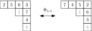
As composition of permutations it is clear that , and from it follows that
i.e. is an involution. Since is order-preserving except for the entries of and have the same relative order except for and . Therefore
As exactly one of or holds, and thus the two permutations and are of different type, i.e. is a type-inverting involution on .
3.2. Case
Given two subsets with , let denote the unique order-preserving bijection between and , i.e. the bijection satisfying for all . Obviously, we have .
If and set , and . The type-inverting involution in this case is
| (3.4) |
Note that is well-defined and an element of (see Figure 16 for an example).
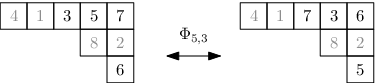
Moreover we have
Therefore and . It follows that
and
i.e. . As in the case the relative order of the last entries of and is the same. The entry is among the smallest elements of if and only if is not among the smallest elements of . Therefore
Since for all , the permutations and are of different type.
3.3. Case
In the case let us define a subset of exceptional permutations which we exclude from the involution: We say that is exceptional if and only if for all . Note that the number of exceptional permutations is . Given , let minimal such that . Define
| (3.5) |
An example can be seen in Figure 17.

Note that is well-defined and since we have and . With it follows that
and
i.e. is an involution. The relative order of the entries in and is the same except for and . Since is among the smallest elements of if and only if is not among the smallest elements of the involution is type-inverting. We can conclude the proof by noting that all exceptional permutations are of the same type, since for all implies that is not among the smallest elements of .
4. Proof of Corollary 1.2 & Examples
The statement of Corollary 1.2 can be observed by computing the number of standard fillings of in two different ways. On the one hand we can use the hook-length formula (1.6) for insets. On the other hand we could refine the counting w.r.t. the left-most entry in the second row: In each standard filling of the left-most entries in the first row are . For let denote the number of standard fillings of where the left-most entry in the second row is (see Figure 18).

Now note that for each fixed the standard fillings counted by are in one-to-one correspondence with standard Young tableaux of shape where the left-most entry in the second row is at least (by considering the entries in and the order-preserving map). Together with , (1.1) and (1.6) we obtain
Let us apply this result to the three families of partitions in Figure 12.
Example 4.1.
Consider the partition . From Corollary 1.2 we obtain
Of course, this could also be obtained by the elementary observation that and
Example 4.2.
Fix and consider the partition . For it follows that
Example 4.3.
Let be of staircase shape. After a short computation one obtains
where denotes the double factorial, i.e. and . By applying Stirling’s formula one can show that asymptotically .
References
- [AIT43] (1943) The monomial expansion of determinantal symmetric functions. Proc. Royal Soc. Edinburgh (A) 61, pp. 300–310. Cited by: §1.5.
- [FIS01] (2001) A bijective proof of the hook-length formula for shifted standard tableaux. arXiv:math. External Links: ISSN 0112261 [ Cited by: §1.2, §1.5.
- [FRT54] (1954) The hook graphs of the symmetric group. Canad. J. Math. 6, pp. 316–324. Cited by: §1.2.
- [GAN78] (1978) Matrix correspondences and the enumeration of plane partitions. Ph.D. Thesis. Cited by: §1.2.
- [IT07] (2007) Schur Function Identities and Hook Length Posets. Note: http://www.fpsac.org/FPSAC07/SITE07/PDF-Proceedings/Posters/55.pdf Cited by: §1.3.
- [NO10] (2010) An algorithm which generates linear extensions for a generalized Young diagram with uniform probability. DMTCS, pp. 801–808. Cited by: §1.5.
- [NAK12] (2012) An algorithm which generates linear extensions for a non-simply laced d-complete poset with uniform probability. DMTCS, pp. 661–666. Cited by: §1.5.
- [NPS97] (1997) A direct bijective proof of the hook-length formula. DMTCS 1, pp. 53–67. Cited by: §1.1, §1.2, §1.5, §2.2.
- [9] http://www.unc.edu/math/Faculty/rap/ (unpublished). Cited by: §1.3.
- [PRO99] (1999) Dynkin Diagram Classification of -Minuscule Bruhat Lattices and of d-Complete Posets. J. Alg. Combin. 9, pp. 61–94. Cited by: §1.3, §1.3, §1.3, §1.5.
- [SAG01] (2001) The symmetric group: representations, combinatorial algorithms, and symmetric functions. Springer. Cited by: §1.2.
- [SCH72] (1972) Promotion des morphismes d’ensembles ordonnés. Discrete Math. 2, pp. 73 –94. Cited by: §1.1.
- [SCH76] (1976) La correspondance de Robinson. Combinatoire et représentation du groupe symétrique (D. Foata), Springer, pp. 59–113. Cited by: §1.1.
- [STA01] (2001) Enumerative Combinatorics, Volume 2. Cambridge University Press. Cited by: §1.5.
- [STA11] (2011) Enumerative Combinatorics, Volume 1, Second Edition. Cambridge University Press. Cited by: §1.3.