On the Design of LIL Tests for (Pseudo) Random Generators and Some Experimental Results
Abstract
Random numbers have been one of the most useful objects in statistics, computer science, cryptography, modeling, simulation, and other applications though it is very difficult to construct true randomness. Many solutions (e.g., cryptographic pseudorandom generators) have been proposed to harness or simulate randomness and many statistical testing techniques have been proposed to determine whether a pseudorandom generator produces high quality randomness. NIST SP800-22 (2010) proposes the state of art testing suite for (pseudo) random generators to detect deviations of a binary sequence from randomness. On the one hand, as a counter example to NIST SP800-22 test suite, it is easy to construct functions that are considered as GOOD pseudorandom generators by NIST SP800-22 test suite though the output of these functions are easily distinguishable from the uniform distribution. Thus these functions are not pseudorandom generators by definition. On the other hand, NIST SP800-22 does not cover some of the important laws for randomness. Two fundamental limit theorems about random binary strings are the central limit theorem and the law of the iterated logarithm (LIL). Several frequency related tests in NIST SP800-22 cover the central limit theorem while no NIST SP800-22 test covers LIL.
This paper proposes techniques to address the above challenges that NIST SP800-22 testing suite faces. Firstly, we propose statistical distance based testing techniques for (pseudo) random generators to reduce the above mentioned Type II errors in NIST SP800-22 test suite. Secondly, we propose LIL based statistical testing techniques, calculate the probabilities, and carry out experimental tests on widely used pseudorandom generators by generating around 30TB of pseudorandom sequences. The experimental results show that for a sample size of 1000 sequences (2TB), the statistical distance between the generated sequences and the uniform distribution is around 0.07 (with for statistically indistinguishable and for completely distinguishable) and the root-mean-square deviation is around 0.005. Though the statistical distance 0.07 and RMSD 0.005 are acceptable for some applications, for a cryptographic “random oracle”, the preferred statistical distance should be smaller than 0.03 and RMSD be smaller than 0.001 at the sample size 1000. These results justify the importance of LIL testing techniques designed in this paper. The experimental results in this paper are reproducible and the raw experimental data are available at author’s website.
I Introduction
Secure cryptographic hash functions such as SHA1, SHA2, and SHA3 and symmetric key block ciphers (e.g., AES and TDES) have been commonly used to design pseudorandom generators with counter modes (e.g., in Java Crypto Library and in NIST SP800-90A standards). Though security of hash functions such as SHA1, SHA2, and SHA3 has been extensively studied from the one-wayness and collision resistant aspects, there has been limited research on the quality of long pseudorandom sequences generated by cryptographic hash functions. Even if a hash function (e.g., SHA1) performs like a random function based on existing statistical tests (e.g., NIST SP800-22 Revision 1A [17]), when it is called many times for a long sequence generation, the resulting long sequence may not satisfy the properties of pseudorandomness and could be distinguished from a uniformly chosen sequence. For example, the recent reports from New York Times [16] and The Guardian [1] show that NSA has included back doors in NIST SP800-90A pseudorandom bit generators (on which our experiments are based on) to get online cryptanalytic capabilities.
Statistical tests are commonly used as a first step in determining whether or not a generator produces high quality random bits. For example, NIST SP800-22 Revision 1A [17] proposed the state of art statistical testing techniques for determining whether a random or pseudorandom generator is suitable for a particular cryptographic application. NIST SP800-22 includes 15 tests: frequency (monobit), number of 1-runs and 0-runs, longest-1-runs, binary matrix rank, discrete Fourier transform, template matching, Maurer’s “universal statistical” test, linear complexity, serial test, the approximate entropy, the cumulative sums (cusums), the random excursions, and the random excursions variants. In a statistical test of [17], a significance level is chosen for each test. For each input sequence, a -value is calculated and the input string is accepted as pseudorandom if -value . A pseudorandom generator is considered good if, with probability , the sequences produced by the generator fail the test. For an in-depth analysis, NIST SP800-22 recommends additional statistical procedures such as the examination of P-value distributions (e.g., using -test).
NIST SP800-22 test suite has inherent limitations with straightforward Type II errors. For example, for a function that mainly outputs “random strings” but, with probability , outputs biased strings (e.g., strings consisting mainly of 0’s), will be considered as a “good” pseudorandom generator by NIST SP800-22 test though the output of could be distinguished from the uniform distribution (thus, is not a pseudorandom generator by definition). In the following, we use two examples to illustrate this kind of Type II errors. Let be the sets of Kolmogorov -random binary strings of length , where . That is, for a universal Turing machine , let
| (1) |
Let be a given significance level of NIST SP800-22 test and where is a size subset of and is a size subset of . Furthermore, let be an ensemble of random functions (not necessarily computable) such that is chosen uniformly at random from . Then for each -bit string , with probability , is Kolmogorov 2-random and with probability , . Since all Kolmogorov -random strings are guaranteed to pass NIST SP800-22 test at significance level (otherwise, they are not Kolmogorov -random by definition) and all strings in fail NIST SP800-22 test at significance level for large enough , the function ensemble is considered as a “good” pseudorandom generator by NIST SP800-22 test suite. On the other hand, Theorem 3.2 in Wang [24] shows that (and ) could be efficiently distinguished from the uniform distribution with a non-negligible probability. A similar argument could be used to show that could be efficiently distinguished from the uniform distribution with a non-negligible probability. In other words, is not a cryptographically secure pseudorandom generator.
As another example, let be a pseudorandom generator with where . Assume that is a good pseudorandom generator by NIST SP800-22 in-depth statistical analysis of the P-value distributions (e.g., using -test). Define a new pseudorandom generators as follows:
| (2) |
Then it is easy to show that is also a good pseudorandom generator by NIST SP800-22 in-depth statistical analysis of the P-value distributions (e.g., using -test). However, the output of is trivially distinguishable from the uniform distribution.
The above two examples show the limitation of testing approaches specified in NIST SP800-22. The limitation is mainly due to the fact that NIST SP800-22 does not fully realize the differences between the two common approaches to pseudorandomness definitions as observed and analyzed in Wang [24]. In other words, the definition of pseudorandom generators is based on the indistinguishability concepts though techniques in NIST SP800-22 mainly concentrate on the performance of individual strings. In this paper, we propose testing techniques that are based on statistical distances such as root-mean-square deviation or Hellinger distance. The statistical distance based approach is more accurate in deviation detection and avoids above type II errors in NIST SP800-22. Our approach is illustrated using the LIL test design.
Feller [6] mentioned that the two fundamental limit theorems of random binary strings are the central limit theorem and the law of the iterated logarithm. Feller [6] also called attention to the study of the behavior of the maximum of the absolute values of the partial sums and Erdos and Kac [5] obtained the limit distribution of . NIST SP800-22 test suite includes several frequency related tests that cover the first central limit theorem and the cusum test, “the cumulative sums (cusums) test”, that covers the limit distribution of . However it does not include any test for the important law of the iterated logarithm. Thus it is important to design LIL based statistical tests. The law of the iterated logarithm (LIL) says that, for a pseudorandom sequence , the value (this value is defined in Theorem III.3) should stay in and reach both ends infinitely often when increases. It is known [21, 22, 23] that polynomial time pseudorandom sequences follow LIL. It is also known [7] that LIL holds for uniform distributions. Thus LIL should hold for both Kolmogorov complexity based randomness and for “behavioristic” approach based randomness.
This paper designs LIL based weak, strong, and snapshot statistical tests and obtains formulae for calculating the probabilities that a random sequence passes the LIL based tests. We have carried out some experiments to test outcomes of several commonly used pseudorandom generators. In particular, we generated 30TB of sequences using several NIST recommended pseudorandom generators. Our results show that at the sample size 1000 (or 2TB of data), sequences produced by several commonly used pseudorandom generators have a LIL based statistical distance 0.07 from true random sources. On the other hand, at the sample size 10000 (20TB of data), sequences produced by NIST-SHA256 based pseudorandom generators have a LIL based statistical distance 0.02 from true random sources. These distances are larger than expected for cryptographic applications.
The paper is organized as follows. Section II introduces notations. Section III discusses the law of iterated logarithms (LIL). Section IV reviews the normal approximation to binomial distributions. Sections V, VI, and VII propose weak and strong LIL tests. Section VIII describes the steps to evaluate a pseudorandom generator. Section introduces Snapshot LIL tests. Section X reports experimental results and we conclude with Section XI.
II Notations and pseudorandom generators
In this paper, and denotes the set of natural numbers (starting from ) and the set of non-negative real numbers, respectively. is the binary alphabet, is the set of (finite) binary strings, is the set of binary strings of length , and is the set of infinite binary sequences. The length of a string is denoted by . is the empty string. For strings , is the concatenation of and , denotes that is an initial segment of . For a sequence and a natural number , denotes the initial segment of length of ( if ) while denotes the th bit of , i.e., . For a set C of infinite sequences, denotes the probability that when is chosen by a uniform random experiment. Martingales are used to describe betting strategies in probability theory.
Definition II.1
(Ville [19]) A martingale is a function such that, for all ,
We say that a martingale succeeds on a sequence if .
The concept of “effective similarity” by Goldwasser and Micali [10] and Yao [25] is defined as follows: Let and be two probability ensembles such that each of and is a distribution over . We say that and are computationally (or statistically) indistinguishable if for every feasible algorithm (or every algorithm ), the total variation difference between and is a negligible function in .
Definition II.2
Let and be two probability ensembles. and are computationally (respectively, statistically) indistinguishable if for any polynomial time computable set (respectively, any set ) and any polynomial , the inequality (3) holds for almost all .
| (3) |
Let with for all and be a polynomial-time computable algorithm such that for all .
Definition II.3
Let with for all , and be the uniform distribution. A pseudorandom generator is a polynomial-time algorithm with the following properties:
- 1.
for all .
- 2.
The ensembles and are computationally indistinguishable.
Let where is the set of Kolmogorov -random sequences that is defined in equation (1). Then we have
Theorem II.4
([24, Theorem 3.2]) The ensemble is not pseudorandom.
Theorem II.4 shows the importance for a good pseudorandom generator to fail each statistical test with certain given probability.
III Stochastic Properties of Long Pseudorandom Sequences
Classical infinite random sequences were first introduced as a type of disordered sequences, called “Kollektivs", by von Mises [20] as a foundation for probability theory. The two features characterizing a Kollektiv are: the existence of limiting relative frequencies within the sequence and the invariance of these limits under the operation of an “admissible place selection". Here an admissible place selection is a procedure for selecting a subsequence of a given sequence in such a way that the decision to select a term does not depend on the value of . Ville [19] showed that von Mises’ approach is not satisfactory by proving that: for each countable set of “admissible place selection" rules, there exists a “Kollektiv" which does not satisfy the law of the iterated logarithm (LIL). Later, Martin-Löf [14] developed the notion of random sequences based on the notion of typicalness. A sequence is typical if it is not in any constructive null sets. Schnorr [18] introduced -randomness concepts by defining the constructive null sets as polynomial time computable measure sets. The law of the iterated logarithm (LIL) plays a central role in the study of the Wiener process and Wang [23] showed that LIL holds for -random sequences.
Computational complexity based pseudorandom sequences have been studied extensively in the literature. For example, -random sequences are defined by taking each polynomial time computable martingale as a statistical test.
Definition III.1
(Schnorr [18]) An infinite sequence is p-random (polynomial time random) if for any polynomial time computable martingale , does not succeed on .
A sequence is Turing machine computable if there exists a Turing machine to calculate the bits , , . In the following, we prove a theorem which says that, for each Turing machine computable non -random sequence , there exists a martingale such that the process of succeeding on can be efficiently observed in time . The theorem is useful in the characterizations of -random sequences and in the characterization of LIL-test waiting period.
Theorem III.2
([23]) For a sequence and a polynomial time computable martingale , succeeds on if and only if there exists a martingale and a non-decreasing -time computable (with respect to the unary representation of numbers) function from such that for all .
It is shown in [23] that -random sequences are stochastic in the sense of von Mises and satisfy common statistical laws such as the law of the iterated logarithm. It is not difficult to show that all -random sequences pass the NIST SP800-22 [17] tests for significance level since each test in [17] could be converted to a polynomial time computable martingale which succeeds on all sequences that do not pass this test. However, none of the sequences generated by pseudorandom generators are -random since from the generator algorithm itself, a martingale can be constructed to succeed on sequences that it generates.
Since there is no efficient mechanism to generate -random sequences, pseudorandom generators are commonly used to produce long sequences for cryptographic applications. While the required uniformity property (see NIST SP800-22 [17]) for pseudorandom sequences is equivalent to the law of large numbers, the scalability property (see [17]) is equivalent to the invariance property under the operation of “admissible place selection” rules. Since -random sequences satisfy common statistical laws, it is reasonable to expect that pseudorandom sequences produced by pseudorandom generators satisfy these laws also (see, e.g., [17]).
The law of the iterated logarithm (LIL) describes the fluctuation scales of a random walk. For a nonempty string , let
where denotes the number of 1s in and denotes the reduced number of 1s in . amounts to measuring the deviations of from in units of .
The law of large numbers says that, for a pseudo random sequence , the limit of is , which corresponds to the frequency (Monobit) test in NIST SP800-22 [17]. But it says nothing about the reduced deviation . It is intuitively clear that, for a pseudorandom sequence , will sooner or later take on arbitrary large values (though slowly). The law of the iterated logarithm (LIL), which was first discovered by Khintchine [12], gives an optimal upper bound for the fluctuations of . It was showed in Wang [23] that this law holds for -random sequences also.
Theorem III.3
(LIL for -random sequences [23]) For a sequence , let
| (4) |
Then for each -random sequence we have both
IV Normal Approximations to
In this section, we provide several results on normal approximations to the function that will be used in next sections. The DeMoivre-Laplace theorem is a normal approximation to the binomial distribution, which says that the number of “successes” in independent coin flips with head probability is approximately a normal distribution with mean and standard deviation . We first review a few classical results on the normal approximation to the binomial distribution.
Definition IV.1
The normal density function with mean and variance is defined as
| (5) |
For and , we have the standard normal density function
| (6) |
its integral
| (7) |
is the standard normal distribution function.
Lemma IV.2
([7, Chapter VII.1, p175]) For every , we have
| (8) |
The following DeMoivre-Laplace limit theorem is derived from the approximation Theorem on page 181 of [7].
Theorem IV.3
For fixed , we have
| (9) |
The growth speed for the above approximation is bounded by where .
The following lemma is useful for interpreting based approximation results into based approximation. It is obtained by noting the fact that .
Lemma IV.4
For any , we have
In this paper, we only consider tests for and . That is, . Thus
Hence, we have
By Theorem IV.3, the approximation probability calculation errors in this paper will be less than which is negligible. Unless stated otherwise, we will not mention the approximation errors in the remainder of this paper.
V Weak-LIL test and design
Theorem III.3 shows that pseudorandom sequences should satisfy the law of the iterated logarithm (LIL). Thus we propose the following weak LIL test for random sequences.
Weak LIL Test: Let and be a subset of natural numbers, we say that a sequence does not pass the weak )-LIL test if for all . Furthermore, denotes the probability that a random sequence passes the weak -LIL test, and is the set of sequences that pass the weak -LIL test.
By the definition, a sequence passes the weak )-LIL test if reaches either or at some points in . In practice, it is important to choose appropriate test point set and calculate the probability for a random sequence to pass the weak -LIL test. In this section we calculate the probability for a sequence to pass the weak -LIL test with the following choices of :
for given and . Specifically, we will consider the cases for and .
Theorem V.1
Let . Then we have
| (10) |
Proof. By (4), we have
| (11) |
Theorem V.1 can be generalized as follows.
Theorem V.2
Let and . Then we have
| (12) |
Proof. We first note that
| (13) |
| (14) |
By adding equations (13) and (14) together, we get (12). The theorem is proved.
Corollary V.3
Let and . For given with and randomly chosen ,
| (15) |
Proof. By Theorem V.2, we have
| (16) |
Thus if, and only if,
| (17) |
By Lemma IV.4, (17) is equivalent to (18).
| (18) |
In other words, (15) holds.
After these preliminary results, we will begin to calculate the probability for a random sequence to pass the weak -LIL test.
| 0.03044 | 0.05085 | 0.05441 | 0.05540 | 0.05544 | 0.05507 | 0.05453 | 0.05394 | 0.05334 | |
| 0.02938 | 0.04918 | 0.05263 | 0.05361 | 0.05365 | 0.05331 | 0.05281 | 0.05226 | ||
| 0.02838 | 0.04762 | 0.05097 | 0.05193 | 0.05199 | 0.05168 | 0.05121 | |||
| 0.02746 | 0.04616 | 0.04942 | 0.05036 | 0.05043 | 0.05014 | ||||
| 0.02661 | 0.04479 | 0.04797 | 0.04888 | 0.04897 | |||||
| 0.02580 | 0.04351 | 0.04660 | 0.04750 | ||||||
| 0.02505 | 0.04230 | 0.04531 | |||||||
| 0.02434 | 0.04116 | ||||||||
| 0.02367 | |||||||||
| 0.02234 | 0.03770 | 0.04016 | 0.04074 | 0.04065 | 0.04029 | 0.03983 | 0.03935 | 0.03886 | |
| 0.02148 | 0.03633 | 0.03871 | 0.03928 | 0.03921 | 0.03888 | 0.03845 | 0.03799 | ||
| 0.02068 | 0.03506 | 0.03737 | 0.03792 | 0.03786 | 0.03756 | 0.03716 | |||
| 0.01995 | 0.03387 | 0.03611 | 0.03666 | 0.03661 | 0.03632 | ||||
| 0.01926 | 0.03277 | 0.03494 | 0.03547 | 0.03544 | |||||
| 0.01862 | 0.03173 | 0.03384 | 0.03437 | ||||||
| 0.01802 | 0.03076 | 0.03281 | |||||||
| 0.01746 | 0.02985 | ||||||||
| 0.01693 | |||||||||
Example V.4
For , , and with , the entry at in Table I list the probability that a random sequence passes the weak -LIL test.
Proof. Let . By Theorem IV.3 and Lemma IV.4,
| (19) |
By substituting (respectively ), and into (19), we obtain the value (respectively ) at the entry in Table I. This completes the proof of the Theorem.
Now we consider the probability for a random sequence to pass the weak -LIL test with as the union of two . First we present the following union theorem.
Theorem V.5
For fixed and , let , , , . We have
| (20) |
Alternatively, we have
| (21) |
Proof. Since we have
where
By symmetry, it suffices to show that
| (22) |
Let . By Corollary V.3, the probability that and is approximately
| (23) |
By substituting and integrating the equation (23) over the interval , we get the equation (22).
The equation (21) could be proved similarly by the following observation: a sequence passes the weak -LIL test if it passes the weak LIL test at point or at point . Thus the total probability is the sum of these two probabilities minus the probability that the sequence passes the weak LIL test at both points at the same time. The theorem is then proved.
Example V.6
For (respectively ) and with , the entry at in Table I is the probability that a random sequence passes the weak -LIL test (respectively, -LIL test).
Proof. The probability could be calculated using either equation (20) or (21) in Theorem V.5 with . Our analysis shows that results from (20) and (21) have a difference smaller than which is negligible. The values in Table I are computed using the equation (20) and then verified using the equation (21).
VI Weak-LIL test design II
In this section, we consider the design of weak -LIL test with consisting at least three points. To be consistent with Section V, we use the following notations: , and for given and . In particular, we will consider the cases for .
Theorem VI.1
For fixed and , let , , and . Then we have
| (24) |
where
Proof. By symmetry, it suffices to show that
| (25) |
By Corollary V.3, the probability that and is approximately
| (26) |
where is the probability that . Let . By equation (22) in the proof of Theorem V.5, the probability under the conditional event “” is approximately
| (27) |
By substituting (27) into (26), replacing with , and integrating the obtained equation (27) over the interval , and finally replacing the variable back to , equation (25) is obtained. The theorem is then proved.
Example VI.2
Theorem VI.1 provides an algorithm for computing the probability when contains three points. By recursively applying Corollary V.3 as in the proof of Theorem VI.1, we can obtain algorithms for calculating the probability when contains more than three points. The process is straightforward though tedious and the details are omitted here. In the following, we give an alternative approach to approximate the probability with by using Theorems V.5 and VI.1.
We show the approximation technique with the example of and . First we note that
| (28) |
Since
we have
| (29) |
Let . By substituting (29) into (28) and simplifying it, we get
| (30) |
On the other hand, we have
Thus we have In other words, a random sequence passes the weak -LIL test with approximately probability.
VII Strong LIL test design
This section considers the following strong LIL tests.
Strong LIL Test: Let and be subsets of natural numbers. We say that a sequence passes the strong )-LIL test if there exist and such that
| (31) |
Alternatively, we say that a sequence passes the strong )-LIL test if there exist such that (31) holds. Furthermore, and denote the probability that a random sequence passes the strong )-LIL and )-LIL tests respectively.
Theorem VII.1
For fixed and , let , , and . We have
| (32) |
Proof. The theorem could be proved in a similar way as in the proof of Theorem V.5.
Example VII.2
Let , , , and . Then we have and
In the following, we provide another approach for obtaining better probability bounds for strong LIL tests. In a negative binomial distribution denote the probability that the th one appears at the position . It is well known that for this distribution, we have mean and variance . Thus the probability that the ’s one appears before the th position is approximated by the following probability:
| (33) |
For and , assume that for given . Then we have
| (34) |
By (34), in order for , we need to have
| (35) |
Let , , and . Using the same argument as in the proof of Theorem V.5 (in particular, the arguments for integrating equation (23)) and the negative binomial distribution equation (33), the probability that a sequence passes the strong -LIL test can be calculated with the following equation.
| (36) |
By substituting the values of , , and , (36) evaluates to 0.0002335. In other words, a random sequence passes the strong -LIL test with probability (this value is same as the value in Example VII.2).
VIII Evaluating Pseudorandom Generators
In order to evaluate the quality of a pseudorandom generator , we first choose a fixed of sequence length, a value , and mutually distinct subsets of . It is preferred that the values on these subsets are as independent as possible (though they are impossible to be independent). For example, we may choose as in Section VI. Then we can carry out the following steps.
- 1.
Set for all .
- 2.
Use to construct a set of binary sequences of length .
- 3.
For each , calculate probability that these sequences pass the weak -LIL test via (respectively, for ).
- 4.
Calculate the average absolute probability distance
and the root-mean-square deviation
where and
- 5.
Decision criteria: the smaller and , the better generator .
IX Snapshot LIL tests and random generator evaluation
We have considered statistical tests based on the limit theorem of the law of the iterated logarithm. These tests do not take full advantage of the distribution , which defines a probability measure on the real line . Let be a set of sequences with a standard probability definition on it. That is, for each , let . Then each set induces a probability measure on by letting
for each Lebesgue measurable set on . For , we use to denote the corresponding probability measure induced by the uniform distribution. By Definition II.2, if is the collection of all length sequences generated by a pseudorandom generator, then the difference between and is negligible.
By Theorem IV.3 and Lemma IV.4, for a uniformly chosen , the distribution of could be approximated by a normal distribution of mean and variance , with error bounded by (see [7]). In other words, the measure can be calculated as
| (37) |
Table V in the Appendix lists values for -length intervals with .
In order to evaluate a pseudorandom generator , first choose a sequence of testing points (e.g., ). Secondly use to generate a set of sequences. Lastly compare the distances between the two probability measures and for .
A generator is considered “good”, if for sufficiently large , the distances between and are negligible (or smaller than a given threshold). There are various definitions of statistical distances for probability measures. In our analysis, we will consider the total variation distance [4]
| (38) |
Hellinger distance [11]
| (39) |
and the root-mean-square deviation
| (40) |
where is a partition of the real line that is defined as
In Section X, we will present some examples of using these distance to evaluate several pseudorandom generators.
X Experimental results
As an example to illustrate the importance of LIL tests, we carry out weak LIL test experiments on pseudorandom generators SHA1PRNG (Java) and NIST DRBG [17] with parameters (and ) and (note that bitsMB and bitsGB).
Before carrying out LIL based tests, we run NIST SP800-22 test tool [15] on sequences that have been generated. The test tool [15] only checks the first 1,215,752,192 bits (145MB) of a sequences since the software uses 4-byte int data type for integer variables. The initial 145MB of each sequence that we have generated passes NIST tests with P-values larger than except for the “longest run of ones in a block” test which failed for several sequences.
X-A Java SHA1PRNG API based sequences


The pseudorandom generator SHA1PRNG API in Java generates sequences , where is an optional seeding string of arbitrary length, the counter is 64 bits long, and is the first 64 bits of . In the experiment, we generated one thousand of sequences with four-byte seeds of integers respectively. For each sequence generation, the “random.nextBytes()” method of SecureRandom Class is called times and a -byte output is requested for each call. This produces sequences of bits long. The LIL test is then run on these sequences and the first picture in Figure 1 shows the LIL-test result curves for the first 100 sequences. To reduce the size of the figure, we use the scale for the -axis. In other words, Figure 1 shows the values for . At this scale, the points are mapped to 82, 116, 164, 232, 328, 463, 655, 927, and 1310 respectively. Table II shows the number of sequences that reach the value 0.9, -0.9, 0.95, and -0.95 at corresponding testing points respectively.
| 82 | 116 | 164 | 232 | 328 | 463 | 655 | 927 | 1310 | |
| Java SHA1PRNG | |||||||||
| 20 | 16 | 20 | 20 | 16 | 14 | 17 | 11 | 11 | |
| 18 | 20 | 18 | 17 | 14 | 11 | 12 | 11 | 9 | |
| 14 | 12 | 13 | 18 | 12 | 10 | 15 | 7 | 8 | |
| 13 | 13 | 14 | 9 | 10 | 7 | 9 | 8 | 6 | |
| NIST SP800 90A SHA1-DRBG at sample size 1000 | |||||||||
| 15 | 16 | 15 | 12 | 8 | 9 | 17 | 10 | 8 | |
| 15 | 19 | 12 | 18 | 10 | 16 | 14 | 9 | ‘2 | |
| 10 | 9 | 12 | 10 | 5 | 5 | 11 | 6 | 6 | |
| 11 | 12 | 8 | 13 | 8 | 10 | 10 | 7 | 12 | |
| NIST SP800 90A SHA256-DRBG at sample size 1000 | |||||||||
| 13 | 16 | 14 | 20 | 13 | 15 | 21 | 16 | 9 | |
| 16 | 13 | 14 | 5 | 13 | 9 | 11 | 13 | 10 | |
| 9 | 10 | 12 | 15 | 9 | 10 | 16 | 14 | 3 | |
| 13 | 9 | 8 | 4 | 8 | 6 | 9 | 12 | 9 | |
| NIST SP800 90A SHA256-DRBG at sample size 10000 | |||||||||
| 164 | 157 | 162 | 145 | 128 | 128 | 133 | 121 | 114 | |
| 154 | 142 | 142 | 130 | 123 | 128 | 123 | 120 | 107 | |
| 120 | 107 | 127 | 110 | 89 | 93 | 93 | 84 | 70 | |
| 107 | 106 | 92 | 99 | 91 | 93 | 95 | 84 | 78 | |
Using the partition set , the probability distributions with are presented in the Appendix Table VI. Figure 2 compares these distributions.
X-B NIST SP800 90A DRBG pseudorandom generators
NIST SP800.90A [2] specifies three types of DRBG generators: hash function based, block cipher based, and ECC based. For DRBG generators, the maximum number of calls between reseeding is for hash function and AES based generators (the number is for T-DES and ECC-DRBG generators). In our experiment, we used hash function based DRBG. where a hash function is used to generate sequences with being seedlen-bit counter that is derived from the secret seeds. The seedlen is for SHA1 and SHA-256 and the value of is revised after at most bits are output. We generated 10000 sequences nistSHADRBG0, , nistSHADRBG9999. For each sequence nistSHADRBG, the seed “th secret seed for NIST DRBG" is used to derive the initial DRBG state and . Each sequence is of the format , where is derived from the value of and . In other words, each is used times before it is revised. The second picture (respectively, the third picture) in Figure 1 shows the LIL-test result curves for the first 100 sequences when SHA1 (respectively, SHA256) is used as the hash function and Table II shows the number of sequences that reach the value 0.9, -0.9, 0.95, and -0.95 at corresponding testing points respectively.
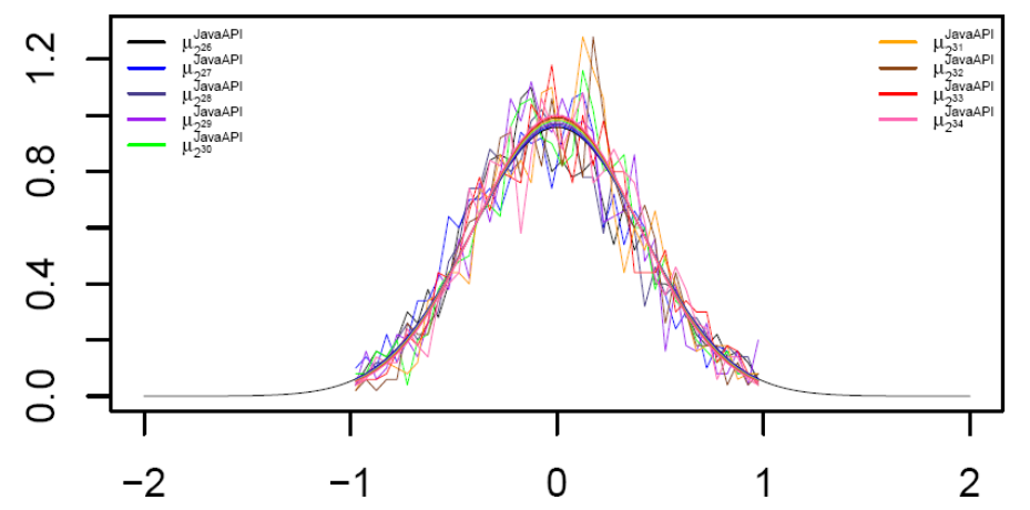
The probability distributions , , and on partition are presented in Appendix Tables VII, VIII, IX respectively. Figure 3 compares the distributions at the sample size 1000. The comparisons for are presented in Appendix Figure 5 and 6.

X-C Comparison and Discussion
Based on Table II, the average absolute probability distance and the root-mean-square deviation at the sample size 1000 (for DRBG-SHA256, we also include results for sample size 10000) are calculated and shown in Table III. These values are quite large.
| Java SHA1PRNG | DRBG-SHA1 | DRBG-SHA256 (1000) | DRBG-SHA256 (10000) | |
| 0.140 | 0.194 | 0.200 | 0.045 | |
| 0.276 | 0.224 | 0.289 | 0.063 | |
| 0.004647 | 0.003741 | 0.004984 | 0.00118 | |
| 0.004042 | 0.003023 | 0.004423 | 0.001107 |
Based on snapshot LIL tests at points , the corresponding total variation distance , Hellinger distance , and the root-mean-square deviation at sample size 1000 (also DRBG-SHA256 at sample size 10,000) are calculated and shown in Table IV, where subscripts are for JavaSHA1, nistDRBGsha1, nistDRBGsha256 (sample size 1000), and nistDRBGsha256 (sample size 10000) respectively. It is observed that at the sample size 1000, the average distance between and is larger than 0.06 and the root-mean-square deviation is around 0.005.
| .074 | .704 | .064 | .085 | .067 | .085 | .074 | .069 | .071 | |
| .062 | .067 | .063 | .089 | .066 | .078 | .077 | .061 | .068 | |
| .005 | .005 | .004 | .005 | .004 | .006 | .005 | .005 | .005 | |
| .066 | .072 | .079 | .067 | .084 | .073 | .065 | .078 | .083 | |
| .060 | .070 | .073 | .062 | .077 | .066 | .067 | .070 | .087 | |
| .004 | .005 | .005 | .004 | .005 | .004 | .004 | .005 | .005 | |
| .076 | .069 | .072 | .093 | .071 | .067 | .078 | .081 | .066 | |
| .082 | .064 | .068 | .088 | .079 | .073 | .076 | .074 | .080 | |
| .005 | .004 | .004 | .006 | .004 | .004 | .005 | .005 | .005 | |
| .021 | .022 | .026 | .024 | .022 | .024 | .026 | .024 | .021 | |
| .019 | .021 | .024 | .024 | .022 | .023 | .025 | .022 | .021 | |
| .001 | .001 | .002 | .001 | .001 | .002 | .002 | .002 | .001 |
Though the statistical distances in Tables III and IV may be acceptable for various applications, for a cryptographic random source at the sample size “1000 of 2GB-long sequences”, it is expected to have a statistical distance smaller than 0.03 and an RMSD smaller than 0.001 for the standard normal distribution (see, e.g., [8]). At sample size 10000 of 2GB sequences, the statistical distance is reduced to 0.02 which is still more than acceptable for cryptographic applications.
One could also visually analyze the pictures in Figure 1. For example, from three pictures in Figure 1, we may get the following impression: sequences generated by Java SHA1PRNG have a good performance to stay within the interval though there is a big gap between 400 and 900 in the bottom area that is close to the line . Among the three pictures, sequences generated by SHA1-DRBG have a better performance that looks more close to a true random source. For sequences generated by SHA2-DRBG, too many sequences reach or go beyond and lines.
XI Conclusion
This paper proposed statistical distance based LIL testing techniques and showed that, at sample size 1000, the collection of sequences generated by several commonly used pseudorandom generators has a statistical distance 0.06 and root-mean-square deviation 0.005 from a true random source. These values are larger than expected for various cryptographic applications. This paper also calculated the probability for weak LIL tests on sequences of less than 2GB. For longer sequences, the corresponding probabilities decrease significantly. Thus large sample sizes of sequences are needed for better LIL testing. Alternatively, one may also split longer sequences into independent sub-sequences of 2GB each and then use the probabilities calculated in this paper to carry out LIL testing on them. For strong LIL tests, this paper obtained a preliminary result with a very small probability for a random sequence to pass. It would be interesting to calculate the exact probability for continuous interval (e.g., ). We believe that is large enough for a reasonable interval such as . When the probability becomes larger, the required sample size for the strong LIL testing will be smaller. It would also be very important to find new techniques that could be used to design pseudorandom generators with smaller statistical distance and smaller root-mean-square deviation from a true random source.
References
- [1] J. Ball, J. Borger, and G. Greenwald. Revealed: how US and UK spy agencies defeat internet privacy and security. http://www.theguardian.com/world/2013/sep/05/nsa-gchq-encryption-codes-security, Sept. 13, 2013.
- [2] E. Barker and J. Kelsey. NIST SP 800-90A: Recommendation for Random Number Generation Using Deterministic Random Bit Generators. NIST, 2012.
- [3] M. Blum and S. Micali. How to generate cryptographically strong sequences of pseudorandom bits. SIAM J. Comput., 13:850–864, 1984.
- [4] J.A. Clarkson and C.R. Adams. On definitions of bounded variation for functions of two variables. Tran. AMS, 35(4):824–854, 1933.
- [5] P. Erdös and M. Kac. On certain limit theorems of the theory of probability. Bulletin of AMS, 52(4):292–302, 1946.
- [6] W. Feller. The fundamental limit theorems in probability. Bulletin of AMS, 51(11):800–832, 1945.
- [7] W. Feller. Introduction to probability theory and its applicatons, volume I. John Wiley Sons, Inc., New York, 1968.
- [8] D. Freedman, R. Pisani, and R. Purves. Statistics. Norton & Company, 2007.
- [9] O. Goldreich. Foundations of cryptography: a primer. Now Publishers Inc, 2005.
- [10] S. Goldwasser and S. Micali. Probabilistic encryption. J. Comput. Sys. Sci., 28(2):270–299, 1984.
- [11] E. Hellinger. Neue begründung der theorie quadratischer formen von unendlichvielen veränderlichen. J. für die reine und angewandte Mathematik, 136:210–271, 1909.
- [12] A. Khintchine. Über einen satz der wahrscheinlichkeitsrechnung. Fund. Math, 6:9–20, 1924.
- [13] A. N. Kolmogorov. Three approaches to the definition of the concept “quantity of information". Problems Inform. Transmission, 1:3–7, 1965.
- [14] P. Martin-Löf. The definition of random sequences. Inform. and Control, 9:602–619, 1966.
- [15] NIST. Test suite, http://csrc.nist.gov/groups/ST/toolkit/rng/, 2010.
- [16] N. Perlroth, J. Larson, and S. Shane. NSA able to foil basic safeguards of privacy on web. http://www.nytimes.com/2013/09/06/us/nsa-foils-much-internet-encryption.html, Sep. 5, 2013.
- [17] A. Rukhin, J. Soto, J. Nechvatal, M. Smid, E. Barker, S. Leigh, M. Levenson, M. Vangel, D. Banks, A. Heckert, J. Dray, and S. Vo. A Statistical Test Suite for Random and Pseudorandom Number Generators for Cryptographic Applications. NIST SP 800-22, 2010.
- [18] C. P. Schnorr. Zufälligkeit und Wahrscheinlichkeit. Lecture Notes in Math. 218. Springer Verlag, 1971.
- [19] J. Ville. Étude Critique de la Notion de Collectif. Gauthiers-Villars, Paris, 1939.
- [20] R. von Mises. Grundlagen der wahrscheinlichkeitsrechung. Math. Z., 5:52–89, 1919.
- [21] Yongge Wang. The law of the iterated logarithm for p-random sequences. In IEEE Conf. Comput. Complexity, pages 180–189, 1996.
- [22] Yongge Wang. Randomness and complexity. PhD Thesis, University of Heidelberg, 1996.
- [23] Yongge Wang. Resource bounded randomness and computational complexity. Theoret. Comput. Sci., 237:33–55, 2000.
- [24] Yongge Wang. A comparison of two approaches to pseudorandomness. Theoretical computer science, 276(1):449–459, 2002.
- [25] A. C. Yao. Theory and applications of trapdoor functions. In Proc. 23rd IEEE FOCS, pages 80–91, 1982.
XII Appendix
Figure 4 shows the distributions of for

and Table V lists values on with . Since is symmetric, it is sufficient to list the distribution in the positive side of the real line.
| .047854 | .048164 | .048460 | .048745 | .049018 | .049281 | .049534 | .049778 | .050013 | |
| .047168 | .047464 | .047748 | .048020 | .048281 | .048532 | .048773 | .049006 | .049230 | |
| .045825 | .046096 | .046354 | 0.04660 | .046839 | .047067 | .047287 | .047498 | .047701 | |
| .043882 | .044116 | .044340 | .044553 | .044758 | .044953 | .045141 | .045322 | .045496 | |
| .041419 | .041609 | .041789 | .041961 | .042125 | .042282 | .042432 | .042575 | .042713 | |
| .038534 | .038674 | .038807 | .038932 | .039051 | .039164 | .039272 | .039375 | .039473 | |
| .035336 | .035424 | .035507 | .035584 | .035657 | .035725 | 0.03579 | .035850 | .035907 | |
| .031939 | .031976 | .032010 | .032041 | .032068 | .032093 | .032115 | .032135 | .032153 | |
| .028454 | .028445 | .028434 | .028421 | .028407 | .028392 | .028375 | .028358 | .028340 | |
| .024986 | .024936 | .024886 | .024835 | .024785 | .024735 | .024686 | .024637 | .024588 | |
| .021627 | .021542 | .021460 | .021379 | .021300 | .021222 | .021146 | .021072 | .020999 | |
| .018450 | .018340 | .018234 | .018130 | .018029 | .017931 | .017836 | .017743 | .017653 | |
| .015515 | .015388 | .015265 | .015146 | .015032 | .014921 | .014813 | .014709 | .014608 | |
| .012859 | .012723 | .012591 | .012465 | .012344 | .012227 | .012114 | .012004 | .011899 | |
| .010506 | .010367 | .010234 | .010106 | .009984 | .009867 | .009754 | .009645 | .009541 | |
| .008460 | .008324 | .008195 | .008072 | .007954 | .007841 | .007733 | .007629 | .007530 | |
| .006714 | .006587 | .006466 | .006351 | .006241 | .006137 | .006037 | .005941 | .005850 | |
| .005253 | .005137 | .005027 | .004923 | .004824 | .004730 | .004640 | .004555 | .004474 | |
| .004050 | .003948 | .003851 | .003759 | .003672 | .003590 | .003512 | .003438 | .003368 | |
| .003079 | .002990 | .002906 | .002828 | .002754 | .002684 | .002617 | .002555 | .002495 | |
| .008090 | .007750 | .007437 | .007147 | .006877 | .006627 | .006393 | .006175 | .005970 |
Table VI lists values on with .
| .011 | .008 | .012 | .007 | .006 | .006 | .008 | .006 | .004 | |
| .002 | .005 | .002 | .002 | .004 | .001 | .001 | .002 | .002 | |
| .005 | .007 | .004 | .008 | .004 | .004 | .003 | .003 | .003 | |
| .008 | .005 | .006 | .003 | .008 | .005 | .001 | .003 | .007 | |
| .007 | .011 | .006 | .005 | .007 | .006 | .003 | .004 | .006 | |
| .010 | .006 | .010 | .011 | .010 | .005 | .003 | .008 | .006 | |
| .015 | .010 | .013 | .010 | .002 | .004 | .013 | .011 | .012 | |
| .013 | .017 | .010 | .007 | .010 | .006 | .011 | .009 | .009 | |
| .019 | .017 | .013 | .013 | .011 | .017 | .011 | .013 | .007 | |
| .014 | .021 | .015 | .022 | .019 | .018 | .017 | .022 | .017 | |
| .020 | .032 | .024 | .019 | .022 | .022 | .021 | .021 | .020 | |
| .030 | .030 | .027 | .028 | .024 | .022 | .027 | .025 | .022 | |
| .034 | .035 | .037 | .021 | .025 | .020 | .031 | .033 | .037 | |
| .036 | .035 | .037 | .038 | .033 | .037 | .032 | .039 | .032 | |
| .042 | .037 | .044 | .031 | .034 | .035 | .035 | .033 | .042 | |
| .043 | .033 | .042 | .039 | .032 | .043 | .046 | .040 | .041 | |
| .042 | .039 | .040 | .053 | .048 | .039 | .047 | .039 | .048 | |
| .053 | .047 | .042 | .049 | .052 | .042 | .039 | .038 | .029 | |
| .055 | .045 | .049 | .056 | .053 | .038 | .048 | .052 | .043 | |
| .047 | .046 | .051 | .049 | .046 | .054 | .041 | .049 | .053 | |
| .040 | .037 | .048 | .047 | .045 | .055 | .053 | .059 | .048 | |
| .042 | .046 | .050 | .053 | .041 | .041 | .041 | .045 | .044 | |
| .039 | .053 | .048 | .048 | .043 | .050 | .049 | .038 | .049 | |
| .040 | .054 | .039 | .049 | .058 | .064 | .039 | .050 | .054 | |
| .042 | .047 | .039 | .047 | .051 | .058 | .064 | .041 | .038 | |
| .034 | .030 | .029 | .031 | .040 | .053 | .050 | .049 | .040 | |
| .027 | .036 | .040 | .032 | .041 | .033 | .039 | .040 | .044 | |
| .034 | .027 | .034 | .033 | .043 | .022 | .033 | .040 | .040 | |
| .026 | .033 | .030 | .043 | .030 | .030 | .030 | .022 | .038 | |
| .030 | .030 | .016 | .024 | .030 | .026 | .034 | .022 | .031 | |
| .020 | .021 | .023 | .028 | .019 | .033 | .028 | .022 | .021 | |
| .020 | .018 | .018 | .008 | .025 | .024 | .013 | .026 | .018 | |
| .019 | .012 | .020 | .020 | .017 | .020 | .022 | .015 | .023 | |
| .015 | .015 | .014 | .009 | .015 | .015 | .015 | .017 | .019 | |
| .011 | .013 | .014 | .008 | .010 | .008 | .009 | .015 | .013 | |
| .009 | .005 | .011 | .013 | .008 | .009 | .009 | .015 | .012 | |
| .011 | .009 | .007 | .004 | .006 | .009 | .009 | .006 | .003 | |
| .007 | .008 | .009 | .004 | .008 | .009 | .002 | .009 | .007 | |
| .008 | .004 | .007 | .008 | .004 | .003 | .006 | .008 | .007 | |
| .006 | .004 | .007 | .002 | .004 | .004 | .002 | .004 | .003 | |
| .003 | .004 | .002 | .010 | .002 | .004 | .004 | .002 | .002 | |
| .011 | .008 | .011 | .008 | .010 | .006 | .011 | .005 | .006 |
Table VII lists values on with .
| .009 | .008 | .007 | .008 | .006 | .007 | .007 | .006 | .007 | |
| .002 | .004 | .001 | .005 | .002 | .003 | .003 | .001 | .005 | |
| .004 | .007 | .004 | .005 | .002 | .006 | .004 | .002 | .000 | |
| .009 | .006 | .011 | .008 | .005 | .003 | .006 | .006 | .009 | |
| .005 | .010 | .004 | .010 | .008 | .003 | .004 | .010 | .003 | |
| .007 | .004 | .010 | .011 | .006 | .008 | .011 | .005 | .002 | |
| .009 | .005 | .014 | .008 | .011 | .017 | .007 | .013 | .011 | |
| .019 | .014 | .014 | .011 | .026 | .015 | .012 | .013 | .009 | |
| .013 | .020 | .010 | .012 | .018 | .011 | .014 | .012 | .011 | |
| .016 | .021 | .019 | .014 | .019 | .022 | .021 | .018 | .017 | |
| .022 | .018 | .022 | .027 | .028 | .022 | .023 | .023 | .023 | |
| .027 | .025 | .020 | .033 | .021 | .029 | .025 | .026 | .034 | |
| .028 | .030 | .024 | .027 | .025 | .033 | .034 | .028 | .035 | |
| .030 | .036 | .031 | .026 | .027 | .026 | .037 | .041 | .036 | |
| .041 | .032 | .037 | .035 | .032 | .026 | .040 | .039 | .038 | |
| .034 | .043 | .052 | .038 | .039 | .032 | .034 | .032 | .048 | |
| .045 | .031 | .048 | .038 | .038 | .046 | .036 | .030 | .044 | |
| .055 | .044 | .048 | .039 | .039 | .042 | .046 | .051 | .050 | |
| .056 | .058 | .046 | .046 | .041 | .050 | .046 | .050 | .042 | |
| .046 | .048 | .048 | .044 | .044 | .051 | .046 | .059 | .039 | |
| .045 | .050 | .035 | .051 | .040 | .053 | .048 | .059 | .048 | |
| .045 | .040 | .051 | .052 | .047 | .041 | .033 | .044 | .042 | |
| .058 | .038 | .060 | .047 | .056 | .044 | .044 | .056 | .051 | |
| .042 | .044 | .035 | .041 | .057 | .047 | .050 | .040 | .048 | |
| .037 | .040 | .040 | .051 | .039 | .049 | .045 | .038 | .033 | |
| .034 | .050 | .037 | .056 | .045 | .039 | .046 | .039 | .033 | |
| .042 | .041 | .034 | .046 | .042 | .032 | .037 | .039 | .035 | |
| .036 | .036 | .040 | .035 | .036 | .031 | .043 | .037 | .040 | |
| .022 | .038 | .028 | .033 | .045 | .029 | .043 | .032 | .038 | |
| .029 | .020 | .026 | .023 | .037 | .036 | .031 | .018 | .034 | |
| .025 | .026 | .028 | .023 | .019 | .029 | .020 | .019 | .026 | |
| .024 | .025 | .034 | .019 | .012 | .031 | .024 | .023 | .031 | |
| .020 | .012 | .016 | .015 | .023 | .020 | .019 | .022 | .014 | |
| .010 | .016 | .011 | .014 | .013 | .019 | .011 | .011 | .015 | |
| .012 | .013 | .011 | .008 | .015 | .012 | .010 | .013 | .013 | |
| .006 | .012 | .011 | .008 | .012 | .011 | .011 | .014 | .006 | |
| .010 | .011 | .005 | .012 | .009 | .006 | .009 | .006 | .011 | |
| .006 | .005 | .006 | .005 | .006 | .005 | .002 | .008 | .006 | |
| .005 | .003 | .006 | .003 | .002 | .005 | .001 | .007 | .005 | |
| .005 | .007 | .003 | .002 | .003 | .004 | .006 | .004 | .002 | |
| .002 | .004 | .003 | .004 | .001 | .001 | .003 | .001 | .001 | |
| .008 | .005 | .010 | .007 | .004 | .004 | .008 | .005 | .005 |
Table VIII lists values on with .
| .007 | .005 | .005 | .002 | .004 | .003 | .003 | .009 | .006 | |
| .006 | .004 | .003 | .002 | .004 | .003 | .006 | .003 | .003 | |
| .003 | .004 | .006 | .001 | .005 | .003 | .002 | .001 | .001 | |
| .004 | .006 | .003 | .005 | .004 | .005 | .002 | .005 | .003 | |
| .007 | .006 | .002 | .013 | .005 | .007 | .011 | .005 | .004 | |
| .008 | .010 | .007 | .006 | .004 | .008 | .013 | .007 | .004 | |
| .007 | .010 | .010 | .013 | .005 | .004 | .009 | .010 | .006 | |
| .021 | .013 | .012 | .015 | .006 | .018 | .011 | .010 | .008 | |
| .009 | .008 | .012 | .015 | .021 | .009 | .014 | .019 | .022 | |
| .016 | .019 | .019 | .018 | .016 | .008 | .020 | .012 | .015 | |
| .025 | .013 | .021 | .016 | .017 | .023 | .021 | .013 | .020 | |
| .014 | .033 | .026 | .023 | .018 | .015 | .025 | .034 | .025 | |
| .028 | .024 | .033 | .023 | .034 | .034 | .030 | .026 | .022 | |
| .021 | .025 | .031 | .034 | .029 | .036 | .032 | .033 | .022 | |
| .034 | .031 | .039 | .043 | .037 | .040 | .024 | .031 | .037 | |
| .042 | .041 | .036 | .027 | .033 | .031 | .036 | .041 | .036 | |
| .043 | .046 | .035 | .030 | .045 | .039 | .039 | .037 | .042 | |
| .040 | .042 | .051 | .047 | .042 | .044 | .036 | .042 | .046 | |
| .039 | .042 | .038 | .050 | .055 | .044 | .053 | .043 | .046 | |
| .048 | .046 | .042 | .055 | .045 | .050 | .045 | .042 | .049 | |
| .049 | .045 | .044 | .043 | .045 | .049 | .040 | .063 | .055 | |
| .055 | .059 | .050 | .062 | .049 | .054 | .056 | .040 | .043 | |
| .043 | .041 | .049 | .044 | .049 | .045 | .059 | .060 | .047 | |
| .046 | .045 | .036 | .038 | .045 | .045 | .042 | .052 | .052 | |
| .049 | .046 | .052 | .040 | .045 | .049 | .048 | .047 | .050 | |
| .054 | .043 | .033 | .046 | .046 | .047 | .033 | .037 | .043 | |
| .044 | .050 | .046 | .041 | .052 | .039 | .038 | .040 | .047 | |
| .037 | .030 | .032 | .033 | .035 | .037 | .034 | .036 | .054 | |
| .033 | .028 | .030 | .040 | .039 | .033 | .036 | .049 | .032 | |
| .025 | .030 | .036 | .027 | .024 | .026 | .029 | .025 | .033 | |
| .022 | .031 | .025 | .043 | .025 | .032 | .027 | .028 | .022 | |
| .023 | .026 | .021 | .016 | .027 | .023 | .018 | .019 | .020 | |
| .017 | .017 | .020 | .012 | .019 | .017 | .028 | .020 | .019 | |
| .024 | .016 | .018 | .014 | .025 | .022 | .018 | .011 | .015 | |
| .008 | .016 | .017 | .009 | .013 | .017 | .014 | .007 | .012 | |
| .013 | .007 | .016 | .014 | .006 | .007 | .014 | .008 | .016 | |
| .002 | .009 | .011 | .010 | .009 | .011 | .004 | .008 | .004 | |
| .011 | .011 | .012 | .007 | .001 | .004 | .005 | .007 | .007 | |
| .010 | .006 | .007 | .003 | .004 | .004 | .004 | .004 | .003 | |
| .004 | .006 | .002 | .005 | .004 | .005 | .005 | .002 | .006 | |
| .002 | .003 | .002 | .007 | .001 | .002 | .005 | .003 | .000 | |
| .007 | .007 | .010 | .008 | .008 | .008 | .011 | .011 | .003 |
Figure 5 compared the distributions .

Table VIII lists values on with .
| .0071 | .0070 | .0062 | .0067 | .0061 | .0066 | .0069 | .0053 | .0055 | |
| .0036 | .0036 | .0030 | .0032 | .0030 | .0027 | .0026 | .0031 | .0023 | |
| .0047 | .0036 | .0050 | .0031 | .0032 | .0035 | .0028 | .0036 | .0029 | |
| .0044 | .0057 | .0060 | .0035 | .0039 | .0047 | .0038 | .0043 | .0035 | |
| .0063 | .0068 | .0058 | .0085 | .0057 | .0062 | .0066 | .0062 | .0050 | |
| .0089 | .0078 | .0090 | .0082 | .0071 | .0057 | .0083 | .0071 | .0070 | |
| .0112 | .0102 | .0103 | .0094 | .0096 | .0097 | .0108 | .0081 | .0099 | |
| .0126 | .0128 | .0118 | .0118 | .0118 | .0113 | .0104 | .0123 | .0120 | |
| .0149 | .0147 | .0166 | .0166 | .0151 | .0147 | .0185 | .0144 | .0147 | |
| .0180 | .0217 | .0179 | .0181 | .0191 | .0180 | .0165 | .0169 | .0199 | |
| .0216 | .0197 | .0215 | .0217 | .0201 | .0247 | .0243 | .0186 | .0188 | |
| .0228 | .0275 | .0245 | .0228 | .0226 | .0220 | .0250 | .0246 | .0255 | |
| .0274 | .0303 | .0310 | .0309 | .0292 | .0283 | .0319 | .0302 | .0287 | |
| .0302 | .0298 | .0322 | .0331 | .0315 | .0326 | .0323 | .0354 | .0336 | |
| .0353 | .0346 | .0344 | .0341 | .0361 | .0385 | .0331 | .0361 | .0329 | |
| .0394 | .0385 | .0365 | .0379 | .0391 | .0408 | .0381 | .0375 | .0387 | |
| .0435 | .0405 | .0391 | .0425 | .0462 | .0375 | .0454 | .0442 | .0446 | |
| .0419 | .0436 | .0430 | .0430 | .0450 | .0488 | .0431 | .0429 | .0453 | |
| .0439 | .0475 | .0446 | .0475 | .0506 | .0450 | .0464 | .0466 | .0491 | |
| .0474 | .0426 | .0516 | .0484 | .0480 | .0499 | .0474 | .0511 | .0501 | |
| .0488 | .0489 | .0473 | .0447 | .0474 | .0471 | .0465 | .0501 | .0481 | |
| .0497 | .0478 | .0499 | .0460 | .0499 | .0505 | .0495 | .0507 | .0485 | |
| .0466 | .0460 | .0470 | .0493 | .0512 | .0465 | .0474 | .0476 | .0469 | |
| .0436 | .0478 | .0479 | .0455 | .0475 | .0481 | .0466 | .0468 | .0494 | |
| .0450 | .0455 | .0467 | .0438 | .0436 | .0459 | .0487 | .0472 | .0469 | |
| .0435 | .0411 | .0389 | .0440 | .0418 | .0466 | .0407 | .0460 | .0431 | |
| .0393 | .0395 | .0392 | .0406 | .0414 | .0390 | .0407 | .0381 | .0405 | |
| .0370 | .0351 | .0325 | .0377 | .0334 | .0341 | .0357 | .0348 | .0352 | |
| .0319 | .0304 | .0323 | .0321 | .0289 | .0300 | .0290 | .0363 | .0347 | |
| .0308 | .0286 | .0295 | .0309 | .0264 | .0274 | .0271 | .0300 | .0293 | |
| .0239 | .0235 | .0249 | .0252 | .0251 | .0243 | .0243 | .0241 | .0257 | |
| .0203 | .0229 | .0184 | .0219 | .0213 | .0226 | .0219 | .0201 | .0202 | |
| .0166 | .0177 | .0166 | .0154 | .0192 | .0168 | .0189 | .0158 | .0178 | |
| .0162 | .0150 | .0160 | .0163 | .0167 | .0154 | .0138 | .0127 | .0144 | |
| .0137 | .0143 | .0145 | .0119 | .0120 | .0122 | .0123 | .0123 | .0111 | |
| .0102 | .0103 | .0111 | .0092 | .0109 | .0103 | .0104 | .0088 | .0091 | |
| .0074 | .0087 | .0089 | .0074 | .0082 | .0079 | .0084 | .0080 | .0070 | |
| .0081 | .0070 | .0075 | .0068 | .0060 | .0063 | .0069 | .0050 | .0067 | |
| .0059 | .0057 | .0047 | .0058 | .0033 | .0050 | .0037 | .0050 | .0040 | |
| .0044 | .0050 | .0035 | .0035 | .0039 | .0035 | .0040 | .0037 | .0044 | |
| .0032 | .0037 | .0033 | .0024 | .0021 | .0027 | .0026 | .0023 | .0015 | |
| .0088 | .0070 | .0094 | .0086 | .0068 | .0066 | .0067 | .0061 | .0055 |
Figure 6 compared the distributions .