跳到论文正文
W Papers独立论文阅读器 arXiv:1401.3301 论文正文 计算阅读时间 · 0%
引用这篇论文根据当前论文元数据生成,正式投稿前建议核对。


License: arXiv.org perpetual non-exclusive license
arXiv:1401.3301v2 [cs.MS] 19 Jun 2015

∎

An efficient way to assemble finite element matrices in vector languages Thanks: This work was partially funded by GNR MoMaS, CoCOA LEFE project, ANR DEDALES and MathSTIC (University Paris 13)

Journal: BIT
François Cuvelier    Caroline Japhet    Gilles Scarella Affiliation: F. Cuvelier Affiliation: Université Paris 13, Sorbonne Paris Cité, LAGA, CNRS UMR 7539, 99 Avenue J-B Clément, F-93430 Villetaneuse, France, E-mail: cuvelier@math.univ-paris13.fr, scarella@math.univ-paris13.fr Affiliation: Université Paris 13, Sorbonne Paris Cité, LAGA, CNRS UMR 7539, 99 Avenue J-B Clément, F-93430 Villetaneuse, France. INRIA Paris-Rocquencourt, BP 105, F-78153 Le Chesnay, France, E-mail: japhet@math.univ-paris13.fr
Received: date / Accepted: date
Abstract

Efficient Matlab codes in 2D and 3D have been proposed recently to assemble finite element matrices. In this paper we present simple, compact and efficient vectorized algorithms, which are variants of these codes, in arbitrary dimension, without the use of any lower level language. They can be easily implemented in many vector languages (e.g. Matlab, Octave, Python, Scilab, R, Julia, C++​ ​ with STL,…). The principle of these techniques is general, we present it for the assembly of several finite element matrices in arbitrary dimension, in the ℙ1{\mathbb{P}_{1}} finite element case. We also provide an extension of the algorithms to the case of a system of PDE’s. Then we give an extension to piecewise polynomials of higher order. We compare numerically the performance of these algorithms in Matlab, Octave and Python, with that in FreeFEM++ and in a compiled language such as C. Examples show that, unlike what is commonly believed, the performance is not radically worse than that of C : in the best/worst cases, selected vector languages are respectively 2.3/3.5 and 2.9/4.1 times slower than C in the scalar and vector cases. We also present numerical results which illustrate the computational costs of these algorithms compared to standard algorithms and to other recent ones.

Keywords: 
finite elements, matrix assembly, vectorization, vector languages, Matlab, Octave, Python
MSC
65N30, 65Y20, 74S05

1 Introduction

Vector languages11 1 which contain usual element-wise operators and functions on multidimensional arrays such as Matlab [27], GNU Octave [30], Python [13], R [14], Scilab [12], Julia [22], C++​ with STL,…, are very widely used for scientific computing (see for example [3, 25, 20, 24, 32]) and there is significant interest in programming techniques in these languages for two reasons. The first concerns how to make clear, compact code to ease implementation and understanding, which is important for teaching and rapid-prototyping in research and industry. The second concerns how to make this compact code fast enough for realistic simulations.

On the other hand, in finite element simulations [4, 5, 21, 33, 35], the need for efficient algorithms for assembling the matrices may be crucial, especially when the matrices may need to be assembled several times. This is the case for example when simulating time-dependent problems with explicit or implicit schemes with time-dependent coefficients (e.g. in ocean-atmosphere coupling or porous medium applications). Other examples are computations with a posteriori estimates when one needs to reassemble the matrix equation on a finer mesh, or in the context of eigenvalue problems where assembling the matrix may be costly. In any event, assembly remains a critical part of code optimization since solution of linear systems, which asymptotically dominates in large-scale computing, could be done with the linear solvers of the different vector languages.

In a vector language, the inclusion of loops is a critical performance degrading aspect and removing them is known as a vectorization. In finite element programming, the classical finite element assembly is based on a loop over the elements (see for example [26]). In [9] T. Davis describes different assembly techniques applied to random matrices of finite element type. A first vectorization technique is proposed in [9]. Other more efficient algorithms in Matlab have been proposed recently in [1, 2, 3, 8, 15, 17, 23, 34].

In this paper we describe vectorized algorithms, which are variants of the codes in [2, 3, 15, 23], extended to arbitrary dimension d≥1d\geq 1, for assembling large sparse matrices in finite element computations. A particular strength of these algorithms is that they make using, reading and extending the codes easier while achieving performance close to that of C.

The aim of this article is the quantitative studies for illustrating the efficiency of the vector languages and the various speed-up of the algorithms, relatively to each other, to C and to FreeFem++ [19]. We also propose a vectorized algorithm in arbitrary dimension which is easily transposable to matrices arising from PDE’s such as (see [33])

−∇⋅(𝔸∇u)+∇⋅(𝒃u)+𝒄⋅∇u+a0u=fin Ω,-\nabla\cdot\left(\mathbb{A}\nabla u\right)+\nabla\cdot\left(\boldsymbol{b}u\right)+\boldsymbol{c}\cdot\nabla u+a_{0}u=f\quad\mbox{in }\Omega, (1)

where Ω\Omega is a bounded domain of ℝd\mathbb{R}^{d} (d≥1d\geq 1), 𝔸∈(L∞​(Ω))d×d,\mathbb{A}\in(L^{\infty}(\Omega))^{d\times d}, 𝒃∈(L∞​(Ω))d,\boldsymbol{b}\in(L^{\infty}(\Omega))^{d}, 𝒄∈(L∞​(Ω))d,\boldsymbol{c}\in(L^{\infty}(\Omega))^{d}, a0∈L∞​(Ω)a_{0}\in L^{\infty}(\Omega) and f∈L2​(Ω)f\in L^{2}(\Omega) are given functions. The description of the vectorized algorithm is done in three steps: we recall (non-vectorized) versions called base and OptV1. The latter requires sparse matrix tools found in most of the languages used for computational science and engineering. Then we give vectorized algorithms which are much faster: OptV2 (memory consuming), OptV (less memory consuming) and OptVS (a symmetrized version of OptV). These algorithms have been tested for several matrices (e.g. weighted mass, stiffness and elastic stiffness matrices) and in different languages. We also provide an extension to the vector case in arbitrary dimension, where the algorithm is applied to the elastic stiffness matrix with variable coefficients, in 2D and 3D.

For space considerations, we restrict ourselves in this paper to ℙ1{\mathbb{P}_{1}} Lagrange finite elements. However, in the appendix we show that with slight modification, the algorithm is valid for piecewise polynomials of higher order.

These algorithms can be efficiently implemented in many languages if the language has a sparse matrix implementation. For the OptV1, OptV2, OptV and OptVS versions, a particular sparse matrix constructor is also needed (see Section 3) and these versions require that the language supports element-wise array operations. Examples of languages for which we obtained an efficient implementation of these algorithms are

  • ∙\bullet

    Matlab,

  • ∙\bullet

    Octave,

  • ∙\bullet

    Python with NumPy and SciPy modules,

  • ∙\bullet

    Scilab,

  • ∙\bullet

    Thrust and Cusp, C++ libraries for CUDA

This paper is organized as follows: in Section 2 we define two examples of finite element matrices. Then we introduce the notation associated to the mesh and to the algorithmic language used in this article. In Section 3 we give the classical and OptV1 algorithms. In Section 4 we present the vectorized OptV2 and OptV algorithms for a generic sparse matrix and ℙ1{\mathbb{P}_{1}} finite elements, with the application to the assemblies of the matrices of Section 2. A similar version called OptVS for symmetric matrices is also given. A first step towards finite elements of higher order is deferred to Appendix B. In Section 5 we consider the extension to the vector case with an application to linear elasticity. In Section 6, benchmark results illustrate the performance of the algorithms in the Matlab, Octave and Python languages. First, we show a comparison between the classical, OptV1, OptV2, OptV and OptVS versions. Then we compare the performances of the OptVS version to those obtained with a compiled language (using SuiteSparse [10] in C language), the latter being well-known to run at high speed and serving as a reference. A comparison is also given with FreeFEM++ [18] as a simple and reliable finite element software. We also show in Matlab and Octave a comparison of the OptVS algorithm and the codes given in [2, 3, 17, 34].

All the computations are done on our reference computer22 2 2 x Intel Xeon E5-2630v2 (6 cores) at 2.60Ghz, 64Go RAM with the releases R2014b for Matlab, 3.8.1 for Octave, 3.4.0 for Python and 3.31 for FreeFEM++. The Matlab/Octave and Python codes may be found in [7].

2 Statement of the problem and notation

In this article we consider the assembly of the standard sparse matrices (e.g. weighted mass, stiffness and elastic stiffness matrices) arising from the ℙ1{\mathbb{P}_{1}} finite element discretization of partial differential equations (see e.g. [5, 33]) in a bounded domain Ω\Omega of ℝd\mathbb{R}^{d} (d≥1d\geq 1).

We suppose that Ω\Omega is equipped with a mesh 𝒯h{\mathcal{T}_{h}} (locally conforming) as described in Table 1. We suppose that the elements belonging to the mesh are dd-simplices . We introduce the finite dimensional space Xh1={v∈𝒞0(Ωh¯),v|K∈ℙ1(K),∀K∈𝒯h}{X_{h}^{1}}=\{v\in{\cal C}^{0}(\overline{{\Omega_{h}}}),\ \ {v}_{|K}\in{\mathbb{P}_{1}}(K),\ \forall K\in{\mathcal{T}_{h}}\} where Ωh=⋃K∈𝒯hK{\Omega_{h}}=\bigcup_{K\in{\mathcal{T}_{h}}}K and ℙ1​(K){\mathbb{P}_{1}}(K) denotes the space of all polynomials over KK and of total degree less than or equal to 11. Let qj{\rm q}^{j}, j=1,…,nqj=1,...,{\mathop{\rm n_{q}}\nolimits} be a vertex of Ωh{\Omega_{h}}, with nq=dim(Xh1){\mathop{\rm n_{q}}\nolimits}=dim({X_{h}^{1}}). The space Xh1{X_{h}^{1}} is spanned by the ℙ1{\mathbb{P}_{1}} Lagrange basis functions {φi}i∈{1,…,nq}\{\varphi_{i}\}_{i\in\left\{{{1},\ldots,{{\mathop{\rm n_{q}}\nolimits}}}\right\}} in ℝd\mathbb{R}^{d}, where φi​(qj)=δi​j\varphi_{i}({\rm q}^{j})=\delta_{ij}, with δi​j\delta_{ij} the Kronecker delta.
We consider two examples of finite element matrices: the weighted mass matrix 𝕄[w]\mathbb{M}^{[w]}, with w∈L∞​(Ω)w\in{L^{\infty}}({\Omega}), defined by

𝕄i,j[w]=∫Ωhwφjφidq,∀(i,j)∈{1,…,nq}2,\mathbb{M}^{[w]}_{i,j}=\int_{\Omega_{h}}w\varphi_{j}\varphi_{i}d{\rm q},\quad\forall(i,j)\in\{1,...,{\mathop{\rm n_{q}}\nolimits}\}^{2}, (2)

and the stiffness matrix 𝕊\mathbb{S} given by

𝕊i,j=∫Ωh⟨∇φj,∇φi⟩dq,∀(i,j)∈{1,…,nq}2.\mathbb{S}_{i,j}=\int_{\Omega_{h}}\left\langle\mathop{\rm\nabla}\nolimits\varphi_{j},\mathop{\rm\nabla}\nolimits\varphi_{i}\right\rangle d{\rm q},\quad\forall(i,j)\in\{1,...,{\mathop{\rm n_{q}}\nolimits}\}^{2}. (3)

Note that on the kk-th element K=TkK=T_{k} of 𝒯h{\mathcal{T}_{h}} we have

∀α∈{1,…,d+1},φi|Tk=λα,with i=me(α,k),\forall{\rm\alpha}\in\left\{{{1},\ldots,{d+1}}\right\},\ \ \ {\varphi_{i}}_{|T_{k}}=\lambda_{\rm\alpha},\ \text{with }i=\mathop{\rm me}\nolimits(\alpha,k), (4)

where (λα)α∈{1,…,d+1}(\lambda_{\rm\alpha})_{{\rm\alpha}\in\left\{{{1},\ldots,{d+1}}\right\}} are the barycentric coordinates (i.e the local ℙ1{\mathbb{P}_{1}} Lagrange basis functions) of KK, and me\mathop{\rm me}\nolimits is the connectivity array (see Table 1). The matrices 𝕄[w]\mathbb{M}^{[w]} and 𝕊\mathbb{S} can be assembled efficiently with a vectorized algorithm proposed in Section 4, which uses the following formula (see e.g. [31])

∫K∏i=1d+1λini​𝑑q=d!​|K|​∏i=1d+1ni!(d+∑i=1d+1ni)!\int_{K}\prod_{i=1}^{d+1}\lambda_{i}^{n_{i}}d{\rm q}=\displaystyle d!|K|\frac{\displaystyle\prod_{i=1}^{d+1}n_{i}!}{\displaystyle(d+\sum_{i=1}^{d+1}n_{i})!} (5)

where |K||K| is the volume of KK and ni∈ℕn_{i}\in\mathbb{N}.

Remark 1

The (non-vectorized or vectorized) finite element assembly algorithms presented in this article may be adapted to compute matrices associated to the bilinear form (1).

Remark 2

These algorithms apply to finite element methods of higher order. Indeed, one can express the ℙk{\mathbb{P}_{k}}-Lagrange basis functions (k≥2k\geq 2) as polynomials in λi\lambda_{i} variable and then use formula (5). In Appendix D we give a first step to obtain a vectorized algorithm for ℙk{\mathbb{P}_{k}} finite elements.

In the remainder of this article, we will use the following notations to describe the triangulation 𝒯h{\mathcal{T}_{h}} of Ω\Omega:

name type dimension description
dd integer 1 dimension of simplices of 𝒯h{\mathcal{T}_{h}}
nq{\mathop{\rm n_{q}}\nolimits} integer 1 number of vertices of 𝒯h{\mathcal{T}_{h}}
nme{\mathop{\rm n_{me}}\nolimits} integer 1 number of mesh elements in 𝒯h{\mathcal{T}_{h}}
q{\rm q} double d×nqd\times{\mathop{\rm n_{q}}\nolimits} array of vertex coordinates
me\mathop{\rm me}\nolimits integer (d+1)×nme(d+1)\times{\mathop{\rm n_{me}}\nolimits} connectivity array
vols{\mathop{\rm vols}\nolimits} double 1×nme1\times{\mathop{\rm n_{me}}\nolimits} array of simplex volumes

Table 1: Data structure associated to the mesh 𝒯h{\mathcal{T}_{h}}

In Table 1, for 𝜈∈{1,…,d}\mathop{\rm\nu}\nolimits\in\{1,\ldots,d\}, q(𝜈,j){{\rm q}}(\mathop{\rm\nu}\nolimits,j) represents the 𝜈\mathop{\rm\nu}\nolimits-th coordinate of the jj-th vertex, j∈{1,…,nq}.j\in\{1,\ldots,{\mathop{\rm n_{q}}\nolimits}\}. The jj-th vertex will be also denoted by qj{\rm q}^{j}. The term me(β,k)\mathop{\rm me}\nolimits({\rm\beta},k) is the storage index of the β{\rm\beta}-th vertex of the kk-th element, in the array qq, for β∈{1,…,d+1}{\rm\beta}\in\{1,...,d+1\} and k∈{1,…,nme}k\in\{1,\ldots,{\mathop{\rm n_{me}}\nolimits}\}.

We also provide below some common functions and operators of the vectorized algorithmic language used in this article which generalize the operations on scalars to higher dimensional arrays, matrices and vectors:

𝔸←𝔹\mathbb{A}\leftarrow\mathbb{B} Assignment
𝔸∗𝔹\mathbb{A}*\mathbb{B} matrix multiplication,
𝔸.∗𝔹\mathbb{A}\boldsymbol{.*}\mathbb{B} element-wise multiplication,
𝔸./𝔹\mathbb{A}\,\boldsymbol{./}\mathbb{B} element-wise division,
𝔸(:)\mathbb{A}(:) all the elements of 𝔸\mathbb{A}, regarded as a single column.
[,][,] Horizontal concatenation,
[;][;] Vertical concatenation,
𝔸(:,J)\mathbb{A}(:,J) JJ-th column of 𝔸\mathbb{A},
𝔸(I,:)\mathbb{A}(I,:) II-th row of 𝔸\mathbb{A},
Sum​(𝔸,d​i​m){\footnotesize{\color[rgb]{0,0,1}\textsc{Sum}}}(\mathbb{A},dim) sums along the dimension d​i​mdim,
𝕀n\mathbb{I}_{n} nn-by-nn identity matrix,
𝟙m×n\mathds{1}_{m\times n} (or 𝟙n\mathds{1}_{n}) mm-by-nn (or nn-by-nn) matrix or sparse matrix of ones,
𝕆m×n\mathds{O}_{m\times n} (or 𝕆n\mathds{O}_{n}) mm-by-nn (or nn-by-nn) matrix or sparse matrix of zeros,
ones​(n1,n2,…,nℓ){\footnotesize{\color[rgb]{0,0,1}\textsc{ones}}}(n_{1},n_{2},...,n_{\ell}) ℓ\ell dimensional array of ones,
zeros​(n1,n2,…,nℓ){\footnotesize{\color[rgb]{0,0,1}\textsc{zeros}}}(n_{1},n_{2},...,n_{\ell}) ℓ\ell dimensional array of zeros.

3 Standard finite element assemblies

In this section we consider the ℙ1{\mathbb{P}_{1}} finite element assembly of a generic nq{\mathop{\rm n_{q}}\nolimits}-by-nq{\mathop{\rm n_{q}}\nolimits} sparse matrix 𝕄\mathbb{M} with its corresponding (d+1)(d+1)-by-(d+1)(d+1) local matrix 𝔼\mathbb{E} (also denoted by 𝔼⁡(K)\mathbb{E}(K) when referring to an element K∈𝒯hK\in{\mathcal{T}_{h}}). For K=TkK=T_{k}, the (α,β)({\rm\alpha},{\rm\beta})-th entry of 𝔼⁡(Tk)\mathbb{E}(T_{k}) is denoted by eα,βke^{k}_{{\rm\alpha},{\rm\beta}}.

In Algorithm 3.1, we recall the classical finite element assembly method for calculating 𝕄\mathbb{M}. In this algorithm, an nq{\mathop{\rm n_{q}}\nolimits}-by-nq{\mathop{\rm n_{q}}\nolimits} sparse matrix 𝕄\mathbb{M} is first declared, then the contribution of each element Tk∈𝒯hT_{k}\in{\mathcal{T}_{h}}, given by a function ElemMat, is added to the matrix 𝕄\mathbb{M}. These successive operations are very expensive due to a suboptimal use of the sparse function.

A first optimized, non-vectorized, version (called OptV1), suggested in [9], is based on the use of the sparse function:

M ←\leftarrow sparse(Ig,Jg,Kg,m,n);


This command returns an m ×\timesn sparse matrix MM such that

M(Ig(k),Jg(k)) ←\leftarrow M(Ig(k),Jg(k)) + Kg(k).


The vectors Ig, Jg and Kg have the same length. The zero elements of K are not taken into account and the elements of Kg having the same indices in Ig and Jg are summed.
Examples of languages containing a sparse function are given below

  • ∙\bullet

    Python (scipy.sparse module) :

    M=sparse.<format>_matrix((Kg,(Ig,Jg)),shape=(m,n))

    where <format> is the sparse matrix format (e.g. csc, csr, lil, …),

  • ∙\bullet

    Matlab : M=sparse(Ig,Jg,Kg,m,n), only csc format,

  • ∙\bullet

    Octave : M=sparse(Ig,Jg,Kg,m,n), only csc format,

  • ∙\bullet

    Scilab : M=sparse([Ig,Jg],Kg,[m,n]), only row-by-row format.

  • ∙\bullet

    C with SuiteSparse [10]

  • ∙\bullet

    CUDA with Thrust [29] and Cusp [28] libraries

The OptV1 version consists in computing and storing all elementary contributions first and then using them to generate the sparse matrix 𝕄\mathbb{M}. The main idea is to create three global 1d-arrays 𝑲g\boldsymbol{K}_{g}, 𝑰g\boldsymbol{I}_{g} and 𝑱g\boldsymbol{J}_{g} of length (d+1)2nme(d+1)^{2}{\mathop{\rm n_{me}}\nolimits}, which store the local matrices as well as the position of their elements in the global matrix as shown on Figure 1. To create the arrays 𝑲g\boldsymbol{K}_{g}, 𝑰g\boldsymbol{I}_{g} and 𝑱g\boldsymbol{J}_{g}, we define three local arrays 𝑲ke,\boldsymbol{K}^{e}_{k}, 𝑰ke\boldsymbol{I}^{e}_{k} and 𝑱ke\boldsymbol{J}^{e}_{k} of length (d+1)2(d+1)^{2} obtained from the (d+1)(d+1)-by-(d+1)(d+1) local matrix 𝔼⁡(Tk)\mathbb{E}(T_{k}) as follows:

𝑲ke\boldsymbol{K}^{e}_{k} : elements of the matrix 𝔼⁡(Tk)\mathbb{E}(T_{k}) stored column-wise,
𝑰ke\boldsymbol{I}^{e}_{k} : global row indices associated to the elements stored in 𝑲ke\boldsymbol{K}^{e}_{k},
𝑱ke\boldsymbol{J}^{e}_{k} : global column indices associated to the elements stored in 𝑲ke.\boldsymbol{K}^{e}_{k}.

Using 𝑲ke\boldsymbol{K}^{e}_{k}, 𝑰ke\boldsymbol{I}^{e}_{k}, 𝑱ke\boldsymbol{J}^{e}_{k} and a loop over the mesh elements Tk,T_{k}, one may calculate the global arrays 𝑰g\boldsymbol{I}_{g}, 𝑱g\boldsymbol{J}_{g} and 𝑲g\boldsymbol{K}_{g}. The corresponding OptV1 algorithm is given in Algorithm 3.2.

Numerical experiments in Section 6.1 and in Tables 9 and 10 show that the OptV1 algorithm is more efficient than the classical one. The inefficiency of the classical (base) version compared to the OptV1 version is mainly due to the repetition of element insertions into the sparse structure and to some dynamic reallocation troubles that may also occur.

However, the OptV1 algorithm still uses a loop over the elements. To improve the efficiency of this algorithm, we propose in the next section other optimized versions, in a vectorized form: the main loop over the elements, which increases with the size of the mesh, is vectorized. The other loops (which are independent of the mesh size and with few iterations) will not necessarily be vectorized.

Refer to caption
Figure 1: Insertion of a local matrix into global 1d-arrays - OptV1 version, where m=d+1,m=d+1, ℐlk=me(l,k)\mathcal{I}^{k}_{l}=\mathop{\rm me}\nolimits(l,k).
Algorithm 3.1 (base) - Classical assembly
1: 𝕄←𝕆nq\mathbb{M}\leftarrow\mathds{O}_{{\mathop{\rm n_{q}}\nolimits}} ⊳\vartriangleright Sparse matrix
2: for k←1k\leftarrow 1 to nme{\mathop{\rm n_{me}}\nolimits} do
3:  𝔼←\mathbb{E}\leftarrow ElemMat(vols(k),…{\mathop{\rm vols}\nolimits}(k),\ldots)
4:  for α←1{\rm\alpha}\leftarrow 1 to d+1d+1 do
5:   i←me(α,k)i\leftarrow\mathop{\rm me}\nolimits({\rm\alpha},k)
6:   for β←1{\rm\beta}\leftarrow 1 to d+1d+1 do
7:    j←me(β,k)j\leftarrow\mathop{\rm me}\nolimits({\rm\beta},k)
8:    𝕄i,j←𝕄i,j+𝔼α,β\mathbb{M}_{i,j}\leftarrow\mathbb{M}_{i,j}+\mathbb{E}_{{\rm\alpha},{\rm\beta}}
9:   end for
10:  end for
11: end for
Algorithm 3.2 (OptV1) - Optimized and non-vectorized assembly
1: 𝑲g←𝑰g←𝑱g←zeros((d+1)2nme,1)\boldsymbol{K}_{g}\leftarrow\boldsymbol{I}_{g}\leftarrow\boldsymbol{J}_{g}\leftarrow{\footnotesize{\color[rgb]{0,0,1}\textsc{zeros}}}((d+1)^{2}{\mathop{\rm n_{me}}\nolimits},1)
2: l←1l\leftarrow 1
3: for k←1k\leftarrow 1 to nme{\mathop{\rm n_{me}}\nolimits} do
4:  𝔼←\mathbb{E}\leftarrow ElemMat(vols(k),…{\mathop{\rm vols}\nolimits}(k),\ldots)
5:  for β←1{\rm\beta}\leftarrow 1 to d+1d+1 do
6:   for α←1{\rm\alpha}\leftarrow 1 to d+1d+1 do
7:    𝑰g​(l)←me(α,k)\boldsymbol{I}_{g}(l)\leftarrow\mathop{\rm me}\nolimits({\rm\alpha},k)
8:    𝑱g​(l)←me(β,k)\boldsymbol{J}_{g}(l)\leftarrow\mathop{\rm me}\nolimits({\rm\beta},k)
9:    𝑲g​(l)←𝔼⁡(α,β)\boldsymbol{K}_{g}(l)\leftarrow\mathbb{E}({\rm\alpha},{\rm\beta})
10:    l←l+1l\leftarrow l+1
11:   end for
12:  end for
13: end for
14: 𝕄←\mathbb{M}\leftarrowsparse(𝑰g\boldsymbol{I}_{g},𝑱g\boldsymbol{J}_{g},𝑲g\boldsymbol{K}_{g},nq{\mathop{\rm n_{q}}\nolimits},nq{\mathop{\rm n_{q}}\nolimits})

4 Optimized finite element assembly

In this section we present optimized algorithms, only available in vector languages. In the first algorithm, OptV2, the idea is to vectorize the main loop over the elements by defining the two-dimensional arrays 𝕂g,\mathbb{K}_{g}, 𝕀g\mathbb{I}_{g} and 𝕁g\mathbb{J}_{g} of size (d+1)2(d+1)^{2}-by-nme{\mathop{\rm n_{me}}\nolimits} which store all the local matrices as well as their positions in the global matrix. Then, as for the OptV1 version, the matrix assembly is obtained with the sparse function:

M ←\leftarrow sparse(𝕀g(:)\mathbb{I}_{g}(:),𝕁g(:)\mathbb{J}_{g}(:),𝕂g(:)\mathbb{K}_{g}(:),nq{\mathop{\rm n_{q}}\nolimits},nq{\mathop{\rm n_{q}}\nolimits});

A non-vectorized approach inspired by OptV1 is as follows: for each mesh element TkT_{k}, the kk-th column of the global arrays 𝕂g,\mathbb{K}_{g}, 𝕀g\mathbb{I}_{g} and 𝕁g\mathbb{J}_{g} is filled with the local arrays 𝑲ke,\boldsymbol{K}^{e}_{k}, 𝑰ke\boldsymbol{I}^{e}_{k}, 𝑱ke\boldsymbol{J}^{e}_{k} respectively, as shown in Figure 2.

Refer to caption
Figure 2: Insertion of a local matrix into global 2D-arrays

Thus, 𝕂g,\mathbb{K}_{g}, 𝕀g\mathbb{I}_{g} and 𝕁g\mathbb{J}_{g} are defined by: ∀k∈{1,…,nme},\forall k\in\left\{{{1},\ldots,{{\mathop{\rm n_{me}}\nolimits}}}\right\}, ∀l∈{1,…,(d+1)2}\forall l\in\left\{{{1},\ldots,{(d+1)^{2}}}\right\},

𝕂g​(l,k)=𝑲ke​(l),𝕀g​(l,k)=𝑰ke​(l),𝕁g​(l,k)=𝑱ke​(l).\displaystyle\mathbb{K}_{g}(l,k)=\boldsymbol{K}^{e}_{k}(l),\quad\quad\mathbb{I}_{g}(l,k)=\boldsymbol{I}^{e}_{k}(l),\quad\quad\mathbb{J}_{g}(l,k)=\boldsymbol{J}^{e}_{k}(l).

A natural way to calculate these three arrays is column-wise. In that case, for each array one needs to compute nme{\mathop{\rm n_{me}}\nolimits} columns.

The OptV2 method consists in calculating these arrays row-wise. In that case, for each array one needs to calculate (d+1)2(d+1)^{2} rows (where dd is independent of the number of mesh elements). This vectorization method is represented in Figure 3.

Refer to caption
Figure 3: Row-wise operations on global 2D-arrays

We first suppose that for α{\rm\alpha} and β{\rm\beta} fixed, we can vectorize the computation of eα,βk,e^{k}_{{\rm\alpha},{\rm\beta}}, for all k∈{1,…,nme}.k\in\left\{{{1},\ldots,{{\mathop{\rm n_{me}}\nolimits}}}\right\}. This vectorization procedure, denoted by vecElem​(α,β,…){\footnotesize\color[rgb]{0.545,0,0}\textsc{vecElem}}({\rm\alpha},{\rm\beta},\ldots), returns a 1d-array containing these nme{\mathop{\rm n_{me}}\nolimits} values. We will describe it in detail for some examples in Sections 4.1 and 4.2. Then we obtain the following algorithm

Algorithm 4.1 (OptV2) - Optimized and vectorized assembly
1: Function 𝕄←\mathbb{M}\leftarrow AssemblyGenP1OptV2(me,nq,…\mathop{\rm me}\nolimits,{\mathop{\rm n_{q}}\nolimits},\ldots)
2:  𝕂g←𝕀g←𝕁g←zeros((d+1)2,nme)\mathbb{K}_{g}\leftarrow\mathbb{I}_{g}\leftarrow\mathbb{J}_{g}\leftarrow{\footnotesize{\color[rgb]{0,0,1}\textsc{zeros}}}((d+1)^{2},{\mathop{\rm n_{me}}\nolimits})⊳\vartriangleright (d+1)2(d+1)^{2}-by-nme{\mathop{\rm n_{me}}\nolimits} 2d-arrays
3:  l←1l\leftarrow 1
4:  for β←1{\rm\beta}\leftarrow 1 to d+1d+1 do
5:   for α←1{\rm\alpha}\leftarrow 1 to d+1d+1 do
6:    𝕂g(l,:)←vecElem(α,β,…)\mathbb{K}_{g}(l,:)\leftarrow{\footnotesize\color[rgb]{0.545,0,0}\textsc{vecElem}}({\rm\alpha},{\rm\beta},\ldots)
7:    𝕀g(l,:)←me(α,:)\mathbb{I}_{g}(l,:)\leftarrow\mathop{\rm me}\nolimits({\rm\alpha},:)
8:    𝕁g(l,:)←me(β,:)\mathbb{J}_{g}(l,:)\leftarrow\mathop{\rm me}\nolimits({\rm\beta},:)
9:    l←l+1l\leftarrow l+1
10:   end for
11:  end for
12:  𝕄←Sparse(𝕀g(:),𝕁g(:),𝕂g(:),nq,nq)\mathbb{M}\leftarrow{\footnotesize{\color[rgb]{0,0,1}\textsc{Sparse}}}(\mathbb{I}_{g}(:),\mathbb{J}_{g}(:),\mathbb{K}_{g}(:),{\mathop{\rm n_{q}}\nolimits},{\mathop{\rm n_{q}}\nolimits})
13: end Function

Algorithm 4.1 is efficient in terms of computation time (see Section 6.1). However it is memory consuming due to the size of the arrays 𝕀g\mathbb{I}_{g}, 𝕁g\mathbb{J}_{g} and 𝕂g\mathbb{K}_{g}. Thus a variant (see [3, 23] for dimension 2 or 3 in Matlab) consists in using the sparse command inside the loops (i.e. for each component of all element matrices). This method, called OptV, is given in Algorithm 4.2.

Algorithm 4.2 (OptV) - Optimized and vectorized assembly (less memory consuming)
1: Function 𝕄←\mathbb{M}\leftarrow AssemblyGenP1OptV(me,nq,…\mathop{\rm me}\nolimits,{\mathop{\rm n_{q}}\nolimits},\ldots)
2:  𝕄←𝕆nq\mathbb{M}\leftarrow\mathbb{O}_{{\mathop{\rm n_{q}}\nolimits}} ⊳\vartriangleright nq{\mathop{\rm n_{q}}\nolimits}-by-nq{\mathop{\rm n_{q}}\nolimits} sparse matrix
3:  for β←1{\rm\beta}\leftarrow 1 to d+1d+1 do
4:   for α←1{\rm\alpha}\leftarrow 1 to d+1d+1 do
5:    𝑲g←vecElem​(α,β,…)\boldsymbol{K}_{g}\leftarrow{\footnotesize\color[rgb]{0.545,0,0}\textsc{vecElem}}({\rm\alpha},{\rm\beta},\ldots)
6:    𝕄←𝕄+Sparse(me(α,:),me(β,:),𝑲g,nq,nq)\mathbb{M}\leftarrow\mathbb{M}+{\footnotesize{\color[rgb]{0,0,1}\textsc{Sparse}}}(\mathop{\rm me}\nolimits({\rm\alpha},:),\mathop{\rm me}\nolimits({\rm\beta},:),\boldsymbol{K}_{g},{\mathop{\rm n_{q}}\nolimits},{\mathop{\rm n_{q}}\nolimits})
7:   end for
8:  end for
9: end Function

For a symmetric matrix, the performance can be improved by using a symmetrized version of OptV (called OptVS), given in Algorithm 4.3. More precisely, in the lines 3-8 of this algorithm, we build a non-triangular sparse matrix which contains the contributions of the strictly upper parts of all the element matrices. In line 9 the strictly lower part contributions are added using the symmetry of the element matrices. Then in lines 10-13 the contributions of the diagonal parts of the element matrices are added.

Algorithm 4.3 (OptVS) - Symmetrized version of OptV
1: Function 𝕄←\mathbb{M}\leftarrow AssemblyGenP1OptVS(me,nq,…\mathop{\rm me}\nolimits,{\mathop{\rm n_{q}}\nolimits},\ldots)
2:  𝕄←𝕆nq\mathbb{M}\leftarrow\mathbb{O}_{{\mathop{\rm n_{q}}\nolimits}} ⊳\vartriangleright nq{\mathop{\rm n_{q}}\nolimits}-by-nq{\mathop{\rm n_{q}}\nolimits} sparse matrix
3:  for α←1{\rm\alpha}\leftarrow 1 to d+1d+1 do
4:   for β←α+1{\rm\beta}\leftarrow{\rm\alpha}+1 to d+1d+1 do
5:    𝑲g←vecElem​(α,β,…)\boldsymbol{K}_{g}\leftarrow{\footnotesize\color[rgb]{0.545,0,0}\textsc{vecElem}}({\rm\alpha},{\rm\beta},\ldots)
6:    𝕄←𝕄+Sparse(me(α,:),me(β,:),𝑲g,nq,nq)\mathbb{M}\leftarrow\mathbb{M}+{\footnotesize{\color[rgb]{0,0,1}\textsc{Sparse}}}(\mathop{\rm me}\nolimits({\rm\alpha},:),\mathop{\rm me}\nolimits({\rm\beta},:),\boldsymbol{K}_{g},{\mathop{\rm n_{q}}\nolimits},{\mathop{\rm n_{q}}\nolimits})
7:   end for
8:  end for
9:  𝕄←𝕄+𝕄t\mathbb{M}\leftarrow\mathbb{M}+\mathbb{M}^{t}
10:  for α←1{\rm\alpha}\leftarrow 1 to d+1d+1 do
11:   𝑲g←vecElem​(α,α,…)\boldsymbol{K}_{g}\leftarrow{\footnotesize\color[rgb]{0.545,0,0}\textsc{vecElem}}({\rm\alpha},{\rm\alpha},\ldots)
12:   𝕄←𝕄+Sparse(me(α,:),me(α,:),𝑲g,nq,nq)\mathbb{M}\leftarrow\mathbb{M}+{\footnotesize{\color[rgb]{0,0,1}\textsc{Sparse}}}(\mathop{\rm me}\nolimits({\rm\alpha},:),\mathop{\rm me}\nolimits({\rm\alpha},:),\boldsymbol{K}_{g},{\mathop{\rm n_{q}}\nolimits},{\mathop{\rm n_{q}}\nolimits})
13:  end for
14: end Function

In the following, our objective is to show using examples how to vectorize the computation of 𝑲g\boldsymbol{K}_{g} (i.e. how to obtain the vecElem function in algorithms OptV2, OptV and OptVS). More precisely for the examples derived from (1), the calculation of 𝑲g\boldsymbol{K}_{g} only depends on the local basis functions and/or their gradients and one may need to calculate them on all mesh elements. For ℙ1{\mathbb{P}_{1}} finite elements, these gradients are constant on each dd-simplex K=Tk.K=T_{k}. Let 𝔾\mathbb{G} be the 3D array of size nme{\mathop{\rm n_{me}}\nolimits}-by-(d+1)(d+1)-by-dd defined by

𝔾(k,α,:)=∇φαk(q),∀α∈{1,…,d+1},∀k∈{1,…,nme}.\displaystyle\mathbb{G}(k,{\rm\alpha},:)=\mathop{\rm\nabla}\nolimits\varphi_{{\rm\alpha}}^{k}({\rm q}),\ \ \forall{\rm\alpha}\in\left\{{{1},\ldots,{d+1}}\right\},\ \forall k\in\left\{{{1},\ldots,{{\mathop{\rm n_{me}}\nolimits}}}\right\}. (6)

In Appendix C, we give a vectorized function called GradientVec (see Algorithm C.1) which computes 𝔾\mathbb{G} in arbitrary dimension. Once the gradients are computed, the local matrices are calculated using the formula (5). For simplicity, in the following we consider the OptV version. The vectorization of the computation of 𝑲g\boldsymbol{K}_{g} is shown using the two examples introduced in Section 2.

4.1 Weighted mass matrix assembly

The local weighted mass matrix 𝕄[w],e​(K)\mathbb{M}^{[w],e}(K) is given by

𝕄α,β[w],e​(K)=∫Kw​λβ​λα​𝑑q,∀(α,β)∈{1,…,d+1}2,\mathbb{M}^{[w],e}_{{\rm\alpha},{\rm\beta}}(K)=\int_{K}w\lambda_{\rm\beta}\lambda_{\rm\alpha}d{\rm q},\quad\forall({\rm\alpha},{\rm\beta})\in\{1,...,d+1\}^{2}, (7)

with w∈L∞​(Ω)w\in{L^{\infty}}({\Omega}). Generally, this matrix cannot be computed exactly and one has to use a quadrature formula. In the following, we choose to approximate ww by wh=πK1⁡(w)w_{h}=\mathop{\pi_{K}^{1}}(w) where πK1⁡(w)=∑γ=1d+1w⁡(qγ)​λγ\mathop{\pi_{K}^{1}}(w)=\sum_{\gamma=1}^{d+1}w({\rm q}^{\gamma})\lambda_{\gamma} is the ℙ1{\mathbb{P}_{1}} Lagrange interpolation of ww. Then using (5), we have the quadrature formula for (7)

∫KπK1⁡(w)​λα​λβ​𝑑q=d!(d+3)!​|K|​(1+δα,β)​(ws+w⁡(qα)+w⁡(qβ)),\int_{K}\mathop{\pi_{K}^{1}}(w)\lambda_{\alpha}\lambda_{\beta}d{\rm q}=\frac{d!}{(d+3)!}|K|(1+\delta_{{\rm\alpha},{\rm\beta}})(w^{s}+w({\rm q}^{{\rm\alpha}})+w({\rm q}^{{\rm\beta}})), (8)

where ws=∑γ=1d+1w⁡(qγ)w^{s}=\sum_{\gamma=1}^{d+1}w({\rm q}^{\gamma}). Using (8) we vectorize the assembly of the approximate weighted mass matrix (2) as shown in Algorithm 4.4.

Algorithm 4.4 (OptV) - Weighted mass matrix assembly
1: Function 𝕄←\mathbb{M}\leftarrow AssemblyMassWP1OptV(me,q,vols,w\mathop{\rm me}\nolimits,{\rm q},{\mathop{\rm vols}\nolimits},w)
2:  𝒘←w⁡(q)\boldsymbol{w}\leftarrow w({\rm q}) ⊳\vartriangleright 1d-array of size nq{\mathop{\rm n_{q}}\nolimits}
3:  𝕎←𝒘⁡(me)\mathbb{W}\leftarrow\boldsymbol{w}(\mathop{\rm me}\nolimits) ⊳\vartriangleright (d+1)(d+1)-by-nme{\mathop{\rm n_{me}}\nolimits} 2d-array
4:  𝒘s←Sum​(𝕎,1)\boldsymbol{w}^{s}\leftarrow{\footnotesize{\color[rgb]{0,0,1}\textsc{Sum}}}(\mathbb{W},1) ⊳\vartriangleright 1d-array of size nme{\mathop{\rm n_{me}}\nolimits}
5:  𝕄←𝕆nq\mathbb{M}\leftarrow\mathbb{O}_{{\mathop{\rm n_{q}}\nolimits}} ⊳\vartriangleright nq{\mathop{\rm n_{q}}\nolimits}-by-nq{\mathop{\rm n_{q}}\nolimits} sparse matrix
6:  for α←1{\rm\alpha}\leftarrow 1 to d+1d+1 do
7:   for β←1{\rm\beta}\leftarrow 1 to d+1d+1 do
8:    𝑲g←d!(d+3)!(1+δα,β)∗vols.∗(𝒘s+𝕎(α,:)+𝕎(β,:))\boldsymbol{K}_{g}\leftarrow\frac{d!}{(d+3)!}(1+\delta_{{\rm\alpha},{\rm\beta}})*{\mathop{\rm vols}\nolimits}\boldsymbol{.*}(\boldsymbol{w}^{s}\boldsymbol{+}\mathbb{W}({\rm\alpha},:)\boldsymbol{+}\mathbb{W}({\rm\beta},:))
9:    𝕄←𝕄+Sparse(me(α,:),me(β,:),𝑲g,nq,nq)\mathbb{M}\leftarrow\mathbb{M}+{\footnotesize{\color[rgb]{0,0,1}\textsc{Sparse}}}(\mathop{\rm me}\nolimits({\rm\alpha},:),\mathop{\rm me}\nolimits({\rm\beta},:),\boldsymbol{K}_{g},{\mathop{\rm n_{q}}\nolimits},{\mathop{\rm n_{q}}\nolimits})
10:   end for
11:  end for
12: end Function

Line 8 of Algorithm 4.4 corresponds to the vectorization of formula (8) and is carried out as follows: first we set 𝒘∈ℝnq\boldsymbol{w}\in\mathbb{R}^{\mathop{\rm n_{q}}\nolimits} such that 𝒘⁡(i)=w⁡(qi),\boldsymbol{w}(i)=w({\rm q}^{i}), 1≤i≤nq1\leq i\leq{\mathop{\rm n_{q}}\nolimits}, or in a vectorized form 𝒘←w⁡(q)\boldsymbol{w}\leftarrow w({\rm q}). Then we compute the array 𝕎\mathbb{W} of size (d+1)(d+1)-by-nme{\mathop{\rm n_{me}}\nolimits} containing, for each dd-simplex, the values of ww at its vertices: 𝕎⁡(α,k)=w⁡(qme(α,k))\mathbb{W}({\rm\alpha},k)=w({\rm q}^{\mathop{\rm me}\nolimits({\rm\alpha},k)}) or in vectorized form 𝕎←𝒘⁡(me).\mathbb{W}\leftarrow\boldsymbol{w}(\mathop{\rm me}\nolimits). We now calculate 𝒘s∈ℝnme\boldsymbol{w}^{s}\in\mathbb{R}^{\mathop{\rm n_{me}}\nolimits} which contains, for each dd-simplex, the sum of the values of ww at its vertices, i.e. we sum 𝕎\mathbb{W} over the rows and obtain line 4 of Algorithm 4.4. Then, formula (8) may be vectorized to obtain line 8 in Algorithm 4.4.

Remark 3

Note that formula (8) is exact if ww is a polynomial of degree 11 on KK. Moreover, if ww is constant, we get the mass matrix (up to the constant ww). Other quadrature rules could be used to approximate the integral in (7) without changing the principle of Algorithm 4.4.

Remark 4

Algorithm 4.4 can be applied to meshes composed of nn-simplices (for n≤dn\leq d) and may be used to compute Neumann or Robin boundary terms.

4.2 Stiffness matrix assembly

The local stiffness matrix 𝕊e​(K)\mathbb{S}^{e}(K) is given, for all (α,β)∈{1,…,d+1}2({\rm\alpha},{\rm\beta})\in\{1,...,d+1\}^{2}, by

𝕊α,βe​(K)=∫K⟨∇λβ,∇λα⟩​𝑑q=|K|​⟨∇λβ,∇λα⟩.\mathbb{S}^{e}_{{\rm\alpha},{\rm\beta}}(K)=\int_{K}\left\langle\mathop{\rm\nabla}\nolimits\lambda_{\rm\beta},\mathop{\rm\nabla}\nolimits\lambda_{\rm\alpha}\right\rangle d{\rm q}=|K|\left\langle\mathop{\rm\nabla}\nolimits\lambda_{\rm\beta},\mathop{\rm\nabla}\nolimits\lambda_{\rm\alpha}\right\rangle. (9)

To obtain the right-hand side of (9) we use the fact that the gradients of the local basis functions are constant on each dd-simplex. The gradients are computed with the vectorized function GradientVec of Algorithm C.1. Then the vectorized assembly Algorithm 4.5 easily follows.

Algorithm 4.5 (OptV) - Stiffness matrix assembly
1: Function 𝕄←\mathbb{M}\leftarrow AssemblyStiffP1OptV(me,q,vols\mathop{\rm me}\nolimits,{\rm q},{\mathop{\rm vols}\nolimits})
2:  𝔾←GradientVec(q,me)\mathbb{G}\leftarrow{\footnotesize\color[rgb]{0.545,0,0}\textsc{GradientVec}}({\rm q},\mathop{\rm me}\nolimits)
3:  𝕄←𝕆nq\mathbb{M}\leftarrow\mathbb{O}_{{\mathop{\rm n_{q}}\nolimits}} ⊳\vartriangleright nq{\mathop{\rm n_{q}}\nolimits}-by-nq{\mathop{\rm n_{q}}\nolimits} sparse matrix
4:  for α←1{\rm\alpha}\leftarrow 1 to d+1d+1 do
5:   for β←1{\rm\beta}\leftarrow 1 to d+1d+1 do
6:    𝑲g←zeros(1,nme)\boldsymbol{K}_{g}\leftarrow{\footnotesize{\color[rgb]{0,0,1}\textsc{zeros}}}(1,{\mathop{\rm n_{me}}\nolimits})
7:    for i←1i\leftarrow 1 to dd do
8:      𝑲g←𝑲g+𝔾(:,β,i).∗𝔾(:,α,i)\boldsymbol{K}_{g}\leftarrow\boldsymbol{K}_{g}\boldsymbol{+}\mathbb{G}(:,{\rm\beta},i)\boldsymbol{.*}\mathbb{G}(:,{\rm\alpha},i)
9:    end for
10:    𝑲g←𝑲g.∗vols\boldsymbol{K}_{g}\leftarrow\boldsymbol{K}_{g}\boldsymbol{.*}{\mathop{\rm vols}\nolimits}
11:    𝕄←𝕄+Sparse(me(α,:),me(β,:),𝑲g,nq,nq)\mathbb{M}\leftarrow\mathbb{M}+{\footnotesize{\color[rgb]{0,0,1}\textsc{Sparse}}}(\mathop{\rm me}\nolimits({\rm\alpha},:),\mathop{\rm me}\nolimits({\rm\beta},:),\boldsymbol{K}_{g},{\mathop{\rm n_{q}}\nolimits},{\mathop{\rm n_{q}}\nolimits})
12:   end for
13:  end for
14: end Function

We will now adapt these methods to the vector case with an application to the assembly of the elastic stiffness matrix in two and three dimensions.

5 Extension to the vector case

In this section we present an extension of Algorithms 4.1 and 4.2 to the vector case, i.e for a system of mm (m>1m>1) partial differential equations such as in elasticity. First, we need to introduce some notation: the space (Xh1)m({X_{h}^{1}})^{m} (where Xh1{X_{h}^{1}} is defined in Section 2), is of dimension ndof=mnq{\mathop{\rm n_{dof}}\nolimits}=m\,{\mathop{\rm n_{q}}\nolimits} and spanned by the vector basis functions {𝝍l,i}1≤i≤nq1≤l≤m\{\boldsymbol{\psi}_{l,i}\}_{\begin{subarray}{c}1\leq i\leq{\mathop{\rm n_{q}}\nolimits}\\ 1\leq l\leq m\end{subarray}}, given by

𝝍l,i=φi​𝒆l,\boldsymbol{\psi}_{l,i}=\varphi_{i}\boldsymbol{e}_{l}, (10)

where {𝒆1,⋯,𝒆m}\{\boldsymbol{e}_{1},\cdots,\boldsymbol{e}_{m}\} is the standard basis of ℝm.\mathbb{R}^{m}. The alternate numbering is chosen for the basis functions. We use either 𝝍l,i\boldsymbol{\psi}_{l,i} or 𝝍s\boldsymbol{\psi}_{s} with s=(i−1)​m+ls=(i-1)m+l to denote them. We will consider the assembly of a generic sparse matrix of dimension ndof{\mathop{\rm n_{dof}}\nolimits}-by-ndof{\mathop{\rm n_{dof}}\nolimits} defined by

ℍr,s=∫Ωhℋ⁡(𝝍s,𝝍r)​𝑑q,\mathbb{H}_{r,s}=\int_{\Omega_{h}}\mathcal{H}(\boldsymbol{\psi}_{s},\boldsymbol{\psi}_{r})d{\rm q},

where ℋ\mathcal{H} is a bilinear differential operator of order one.

As in the scalar case, in order to vectorize the assembly of the matrix, one has to vectorize the computation of the local matrices. To define the local matrix, we introduce the following notation: on the kk-th element K=TkK=T_{k} of 𝒯h{\mathcal{T}_{h}} we denote by {𝝀ł,α}1≤l≤m1≤α≤d+1\{\boldsymbol{\lambda}_{\l,{\rm\alpha}}\}_{\begin{subarray}{c}1\leq l\leq m\\ 1\leq{\rm\alpha}\leq d+1\end{subarray}} the ndfe=m(d+1){\mathop{\rm n_{dfe}}\nolimits}=m(d+1) local basis functions defined by

𝝀ł,α=λα​𝒆l.\boldsymbol{\lambda}_{\l,{\rm\alpha}}=\lambda_{\rm\alpha}\boldsymbol{e}_{l}. (11)

We also use notation 𝝀i\boldsymbol{\lambda}_{i} with i=(α−1)​m+li=({\rm\alpha}-1)m+l to denote 𝝀l,α.\boldsymbol{\lambda}_{l,{\rm\alpha}}. By construction, we have ∀l∈{1,…,m},\forall l\in\left\{{{1},\ldots,{m}}\right\}, ∀α∈{1,…,d+1}\forall{\rm\alpha}\in\left\{{{1},\ldots,{d+1}}\right\}

𝝍l,me(α,k)=𝝀ł,αon​K=Tk.\boldsymbol{\psi}_{l,\mathop{\rm me}\nolimits({\rm\alpha},k)}=\boldsymbol{\lambda}_{\l,{\rm\alpha}}\ \ \mbox{on}\ K=T_{k}.

Thus, the local matrix ℍe\mathbb{H}^{e} on the dd-simplex KK is of size ndfe{\mathop{\rm n_{dfe}}\nolimits}-by-ndfe{\mathop{\rm n_{dfe}}\nolimits}, and is given by

ℍi,je=∫Kℋ⁡(𝝀j,𝝀i)​𝑑q.\mathbb{H}^{e}_{i,j}=\int_{K}\mathcal{H}(\boldsymbol{\lambda}_{j},\boldsymbol{\lambda}_{i})d{\rm q}.

Then, a classical non-vectorized algorithm is given in Algorithm 5.1. The function  ElemH is used to calculate the matrix ℍe\mathbb{H}^{e} for a given dd-simplex KK. As in the scalar case, the vectorized assembly algorithm is based on the use of a function called vecHe which returns the values corresponding to the (i,j)(i,j)-th entry (with (i,j)=(m⁡(α−1)+l,m⁡(β−1)+n)(i,j)=(m({\rm\alpha}-1)+l,m({\rm\beta}-1)+n)) of the local matrices ℍe​(K),\mathbb{H}^{e}(K), for all K∈𝒯hK\in{\mathcal{T}_{h}} and for all l,α,n,β.l,{\rm\alpha},n,{\rm\beta}. We suppose that this function can be vectorized. Then we obtain the OptV2 vectorized assembly of the matrix ℍ\mathbb{H} given in Algorithm 5.2.

Algorithm 5.1 (base) - Classical assembly in vector case (m>1m>1)
1: ndof←m∗nq{\mathop{\rm n_{dof}}\nolimits}\leftarrow m*{\mathop{\rm n_{q}}\nolimits}
2: ℍ←𝕆ndof\mathbb{H}\leftarrow\mathds{O}_{{\mathop{\rm n_{dof}}\nolimits}} ⊳\vartriangleright Sparse matrix
3: for k←1k\leftarrow 1 to nme{\mathop{\rm n_{me}}\nolimits} do
4:  ℍe←\mathbb{H}^{e}\leftarrow ElemH(vols(k),…{\mathop{\rm vols}\nolimits}(k),\ldots)
5:  for l←1l\leftarrow 1 to mm do
6:   for n←1n\leftarrow 1 to mm do
7:    for α←1{\rm\alpha}\leftarrow 1 to d+1d+1 do
8:      r←m∗(me(α,k)−1)+lr\leftarrow m*(\mathop{\rm me}\nolimits({\rm\alpha},k)-1)+l
9:      i←m∗(α−1)+li\leftarrow m*({\rm\alpha}-1)+l
10:      for β←1{\rm\beta}\leftarrow 1 to d+1d+1 do
11:       s←m∗(me(β,k)−1)+ns\leftarrow m*(\mathop{\rm me}\nolimits({\rm\beta},k)-1)+n
12:       j←m∗(β−1)+nj\leftarrow m*({\rm\beta}-1)+n
13:       ℍr,s←ℍr,s+ℍi,je\mathbb{H}_{r,s}\leftarrow\mathbb{H}_{r,s}+\mathbb{H}^{e}_{i,j}
14:      end for
15:    end for
16:   end for
17:  end for
18: end for
Algorithm 5.2 (OptV2) - Optimized assembly in vector case (m>1m>1)
1: ndfe←m∗(d+1){\mathop{\rm n_{dfe}}\nolimits}\leftarrow m*(d+1)
2: 𝕂g←𝕀g←𝕁g←zeros(ndfe2,nme)\mathbb{K}_{g}\leftarrow\mathbb{I}_{g}\leftarrow\mathbb{J}_{g}\leftarrow{\footnotesize{\color[rgb]{0,0,1}\textsc{zeros}}}({\mathop{\rm n^{2}_{dfe}}\nolimits},{\mathop{\rm n_{me}}\nolimits})
3: p←1p\leftarrow 1
4: for l←1l\leftarrow 1 to mm do
5:  for n←1n\leftarrow 1 to mm do
6:   for β←1{\rm\beta}\leftarrow 1 to d+1d+1 do
7:    for α←1{\rm\alpha}\leftarrow 1 to d+1d+1 do
8:      𝕂g(p,:)←vecHe(l,α,n,β,…)\mathbb{K}_{g}(p,:)\leftarrow{\footnotesize\color[rgb]{0.545,0,0}\textsc{vecHe}}(l,{\rm\alpha},n,{\rm\beta},\ldots)
9:      𝕀g(p,:)←m∗(me(α,:)−1)+l\mathbb{I}_{g}(p,:)\leftarrow m*(\mathop{\rm me}\nolimits({\rm\alpha},:)-1)+l
10:      𝕁g(p,:)←m∗(me(β,:)−1)+n\mathbb{J}_{g}(p,:)\leftarrow m*(\mathop{\rm me}\nolimits({\rm\beta},:)-1)+n
11:      p←p+1p\leftarrow p+1
12:    end for
13:   end for
14:  end for
15: end for
16: ndof←m∗nq{\mathop{\rm n_{dof}}\nolimits}\leftarrow m*{\mathop{\rm n_{q}}\nolimits}
17: ℍ←sparse(𝕀g(:),𝕁g(:),𝕂g(:),ndof,ndof)\mathbb{H}\leftarrow\tiny{{\footnotesize{\color[rgb]{0,0,1}\textsc{sparse}}}(\mathbb{I}_{g}(:),\mathbb{J}_{g}(:),\mathbb{K}_{g}(:),{\mathop{\rm n_{dof}}\nolimits},{\mathop{\rm n_{dof}}\nolimits})}

As in Section 4, although Algorithm 5.2 is efficient in terms of computation time, it is memory consuming due to the size of the arrays 𝕀g\mathbb{I}_{g}, 𝕁g\mathbb{J}_{g} and 𝕂g\mathbb{K}_{g}. Thus a variant consists in using the sparse command inside the loops, which leads to the extension of the OptV algorithm to the vector case, given in Algorithm 5.3.

Algorithm 5.3 (OptV) - Optimized assembly in vector case (m>1m>1)
1: Function 𝕄←\mathbb{M}\leftarrow AssemblyVecGenP1OptV(me,nq,…\mathop{\rm me}\nolimits,{\mathop{\rm n_{q}}\nolimits},\ldots)
2:  ndof←m∗nq{\mathop{\rm n_{dof}}\nolimits}\leftarrow m*{\mathop{\rm n_{q}}\nolimits}
3:  𝕄←𝕆ndof\mathbb{M}\leftarrow\mathbb{O}_{{\mathop{\rm n_{dof}}\nolimits}} ⊳\vartriangleright ndof{\mathop{\rm n_{dof}}\nolimits}-by-ndof{\mathop{\rm n_{dof}}\nolimits} sparse matrix
4:  for l←1l\leftarrow 1 to mm do
5:   for α←1{\rm\alpha}\leftarrow 1 to d+1d+1 do
6:    𝑰g←m∗(me(α,:)−1)+l\boldsymbol{I}_{g}\leftarrow m*(\mathop{\rm me}\nolimits({\rm\alpha},:)-1)+l
7:    for n←1n\leftarrow 1 to mm do
8:      for β←1{\rm\beta}\leftarrow 1 to d+1d+1 do
9:       𝑲g←vecHe​(l,α,n,β,…)\boldsymbol{K}_{g}\leftarrow{\footnotesize\color[rgb]{0.545,0,0}\textsc{vecHe}}(l,{\rm\alpha},n,{\rm\beta},\ldots)
10:       𝑱g←m∗(me(β,:)−1)+n\boldsymbol{J}_{g}\leftarrow m*(\mathop{\rm me}\nolimits({\rm\beta},:)-1)+n
11:       𝕄←𝕄+Sparse(𝑰g,𝑱g,𝑲g,ndof,ndof)\mathbb{M}\leftarrow\mathbb{M}+{\footnotesize{\color[rgb]{0,0,1}\textsc{Sparse}}}(\boldsymbol{I}_{g},\boldsymbol{J}_{g},\boldsymbol{K}_{g},{\mathop{\rm n_{dof}}\nolimits},{\mathop{\rm n_{dof}}\nolimits})
12:      end for
13:    end for
14:   end for
15:  end for
16: end Function

For a symmetric matrix, the performance can be improved by using a symmetrized version of Algorithm 5.3 (as in Section 4), given in Algorithm C.2.

In the following the vectorized function vecHe is detailed for the elastic stiffness matrix in 2D and 3D.

5.1 Elastic stiffness matrix assembly

Here we consider sufficiently regular vector fields 𝒖=(u1,…,ud):Ω→ℝd\boldsymbol{u}=(u_{1},\ldots,u_{d}):\Omega\rightarrow\mathbb{R}^{d}, with the associated discrete space (Xh1)d({X_{h}^{1}})^{d}, d=2d=2 or 33 (i.e. m=dm=d in that case).

We consider the elastic stiffness matrix arising in linear elasticity when Hooke’s law is used and the material is isotropic, under small strain hypothesis (see for example [11]). This sparse matrix 𝕂\mathbb{K} is defined by

𝕂l,n=∫Ωhϵ¯t(𝝍n)ℂϵ¯(𝝍l)dq,∀(l,n)∈{1,…,ndof}2,\mathbb{K}_{l,n}=\int_{{\Omega_{h}}}\underline{\boldsymbol{\epsilon}}^{t}(\boldsymbol{\psi}_{n})\mathbb{C}\underline{\boldsymbol{\epsilon}}(\boldsymbol{\psi}_{l})d{\rm q},\ \ \forall(l,n)\in\left\{{{1},\ldots,{{\mathop{\rm n_{dof}}\nolimits}}}\right\}^{2}, (12)

where ϵ¯\underline{\boldsymbol{\epsilon}} is the linearized strain tensor given by

ϵ¯​(𝒖)=12​(∇(𝒖)+∇t(𝒖)),\underline{\boldsymbol{\epsilon}}(\boldsymbol{u})=\frac{1}{2}\left(\boldsymbol{\mathop{\rm\nabla}\nolimits}(\boldsymbol{u})+\boldsymbol{\mathop{\rm\nabla}\nolimits}^{t}(\boldsymbol{u})\right),

with ϵ¯=(ϵ11,ϵ22,2​ϵ12)t\underline{\boldsymbol{\epsilon}}=(\epsilon_{11},\epsilon_{22},2\epsilon_{12})^{t} in 2D and ϵ¯=(ϵ11,ϵ22,ϵ33,2​ϵ12,2​ϵ23,2​ϵ13)t\underline{\boldsymbol{\epsilon}}=(\epsilon_{11},\epsilon_{22},\epsilon_{33},2\epsilon_{12},2\epsilon_{23},2\epsilon_{13})^{t} in 3D, with ϵi​j​(𝒖)=12​(∂ui∂xj+∂uj∂xi)\epsilon_{ij}(\boldsymbol{u})=\frac{1}{2}\left(\frac{\partial u_{i}}{\partial x_{j}}+\frac{\partial u_{j}}{\partial x_{i}}\right). The elasticity tensor ℂ\mathbb{C} depends on the Lamé parameters λ\lambda and μ\mu satisfying λ+μ>0,\lambda+\mu>0, and possibly variable in Ω\Omega. For d=2d=2 or d=3d=3, the matrix ℂ\mathbb{C} is given by

ℂ=(λ​𝟙2+2​μ​𝕀2𝕆2×1𝕆1×2μ)3×3,ℂ=(λ​𝟙3+2​μ​𝕀3𝕆3×3𝕆3×3μ​𝕀3)6×6.\mathbb{C}=\begin{pmatrix}\lambda\mathds{1}_{2}+2\mu\mathbb{I}_{2}&\ \mathds{O}_{2\times 1}\\ \mathds{O}_{1\times 2}&\mu\end{pmatrix}_{3\times 3},\qquad\mathbb{C}=\begin{pmatrix}\lambda\mathds{1}_{3}+2\mu\mathbb{I}_{3}&\ \mathds{O}_{3\times 3}\\ \mathds{O}_{3\times 3}&\mu\mathbb{I}_{3}\end{pmatrix}_{6\times 6}.

Formula (12) is related to the Hooke’s law

𝝈¯=ℂ​ϵ¯,\underline{\boldsymbol{\sigma}}=\mathbb{C}\underline{\boldsymbol{\epsilon}},

where 𝝈¯\underline{\boldsymbol{\sigma}} is the elastic stress tensor.

The vectorization of the assembly of the elastic stiffness matrix (12) will be carried out as in Section 4, through the vectorization of the local elastic stiffness matrix 𝕂e\mathbb{K}^{e} given for all (i,j)∈{1,…,ndfe}2(i,j)\in\left\{{{1},\ldots,{{\mathop{\rm n_{dfe}}\nolimits}}}\right\}^{2} by

𝕂i,je​(K)=∫Kϵ¯t​(𝝀j)​ℂ​ϵ¯​(𝝀i)​𝑑q,\mathbb{K}^{e}_{i,j}(K)=\int_{K}\underline{\boldsymbol{\epsilon}}^{t}(\boldsymbol{\lambda}_{j})\mathbb{C}\underline{\boldsymbol{\epsilon}}(\boldsymbol{\lambda}_{i})d{\rm q}, (13)

or equivalently, using (11), we have for 1≤α,β≤d+11\leq{\rm\alpha},{\rm\beta}\leq d+1 and 1≤l,n≤m1\leq l,n\leq m

𝕂i,je​(K)=∫Kϵ¯t​(𝝀n,β)​ℂ​ϵ¯​(𝝀l,α)​𝑑q,\mathbb{K}^{e}_{i,j}(K)=\int_{K}\underline{\boldsymbol{\epsilon}}^{t}(\boldsymbol{\lambda}_{n,\beta})\mathbb{C}\underline{\boldsymbol{\epsilon}}(\boldsymbol{\lambda}_{l,{\rm\alpha}})d{\rm q}, (14)

with i=(α−1)​d+li=({\rm\alpha}-1)d+l and j=(β−1)​d+nj=({\rm\beta}-1)d+n. The vectorization of 𝕂e\mathbb{K}^{e} is based on the following result:

Lemma 1

There exist two matrices ℚn,l\mathbb{Q}^{n,l} and 𝕊n,l\mathbb{S}^{n,l} of size dd-by-dd depending only on nn and ll such that

ϵ¯t​(𝝀n,β)​ℂ​ϵ¯​(𝝀l,α)\displaystyle\underline{\boldsymbol{\epsilon}}^{t}(\boldsymbol{\lambda}_{n,{\rm\beta}})\mathbb{C}\underline{\boldsymbol{\epsilon}}(\boldsymbol{\lambda}_{l,{\rm\alpha}}) =λ⁡⟨∇λβ,ℚn,l​∇λα⟩+μ⁡⟨∇λβ,𝕊n,l​∇λα⟩.\displaystyle=\lambda\left\langle\mathop{\rm\nabla}\nolimits\lambda_{\rm\beta},\mathbb{Q}^{n,l}\mathop{\rm\nabla}\nolimits\lambda_{\rm\alpha}\right\rangle+\mu\left\langle\mathop{\rm\nabla}\nolimits\lambda_{\rm\beta},\mathbb{S}^{n,l}\mathop{\rm\nabla}\nolimits\lambda_{\rm\alpha}\right\rangle. (15)

The proof of Lemma 1 is given in Appendix B.
Using (15) in (14), we have

𝕂i,je​(K)\displaystyle\mathbb{K}^{e}_{i,j}(K) =⟨∇λβ,ℚn,l​∇λα⟩​∫Kλ​𝑑q+⟨∇λβ,𝕊n,l​∇λα⟩​∫Kμ​𝑑q.\displaystyle=\left\langle\mathop{\rm\nabla}\nolimits\lambda_{\rm\beta},\mathbb{Q}^{n,l}\mathop{\rm\nabla}\nolimits\lambda_{\rm\alpha}\right\rangle\int_{K}\lambda d{\rm q}+\left\langle\mathop{\rm\nabla}\nolimits\lambda_{\rm\beta},\mathbb{S}^{n,l}\mathop{\rm\nabla}\nolimits\lambda_{\rm\alpha}\right\rangle\int_{K}\mu d{\rm q}.

One possibility is to approximate the Lamé parameters λ\lambda and μ\mu by their ℙ1{\mathbb{P}_{1}} finite element interpolation πK1⁡(λ)\mathop{\pi_{K}^{1}}(\lambda) and πK1⁡(μ)\mathop{\pi_{K}^{1}}(\mu), respectively (we consider ℙ1{\mathbb{P}_{1}} instead of ℙ0{\mathbb{P}_{0}} to illustrate better the vectorization, the latter being a special case of the former). Then we have

𝕂i,je​(K)\displaystyle\mathbb{K}^{e}_{i,j}(K) ≈|K|d+1​(⟨∇λβ,ℚn,l​∇λα⟩​λs+⟨∇λβ,𝕊n,l​∇λα⟩​μs),\displaystyle\approx\frac{|K|}{d+1}\left(\left\langle\mathop{\rm\nabla}\nolimits\lambda_{\rm\beta},\mathbb{Q}^{n,l}\mathop{\rm\nabla}\nolimits\lambda_{\rm\alpha}\right\rangle\lambda^{s}+\left\langle\mathop{\rm\nabla}\nolimits\lambda_{\rm\beta},\mathbb{S}^{n,l}\mathop{\rm\nabla}\nolimits\lambda_{\rm\alpha}\right\rangle\mu^{s}\right), (16)

with λs=∑γ=1d+1λ⁡(qγ)\lambda^{s}=\sum_{{\rm\gamma}=1}^{d+1}\lambda({\rm q}^{\rm\gamma}) and μs=∑γ=1d+1μ⁡(qγ).\mu^{s}=\sum_{{\rm\gamma}=1}^{d+1}\mu({\rm q}^{\rm\gamma}). The previous formula may now be vectorized as shown in Algorithm 5.4. This algorithm is based on the vectorization of the computation of the terms ⟨∇λβ,𝔸​∇λα⟩\left\langle\mathop{\rm\nabla}\nolimits\lambda_{\rm\beta},\mathbb{A}\mathop{\rm\nabla}\nolimits\lambda_{\rm\alpha}\right\rangle, which is carried out with the function dotMatVecG in Algorithm 5.5, for any dd-by-dd matrix 𝔸\mathbb{A} independent of the dd-simplices of the mesh. In this algorithm, 𝔾\mathbb{G} is the array of gradients defined in (6), α{\rm\alpha} and β{\rm\beta} are indices in {1,…,d+1}\left\{{{1},\ldots,{d+1}}\right\}, and 𝑿\boldsymbol{X} is a 11-by-nme{\mathop{\rm n_{me}}\nolimits} array such that 𝑿⁡(k)=⟨∇λβ,𝔸​∇λα⟩\boldsymbol{X}(k)=\left\langle\mathop{\rm\nabla}\nolimits\lambda_{\rm\beta},\mathbb{A}\mathop{\rm\nabla}\nolimits\lambda_{\rm\alpha}\right\rangle on K=Tk.K=T_{k}.

Algorithm 5.4 Elastic stiffness matrix assembly - OptV version
1: Function 𝕄←\mathbb{M}\leftarrow AssemblyStiffElasP1OptV(me,q,vols,lamb,mu\mathop{\rm me}\nolimits,{\rm q},{\mathop{\rm vols}\nolimits},{\texttt{lamb}},{\texttt{mu}})
2:  [ℚ,𝕊]←MatQS​(d)[\mathbb{Q},\mathbb{S}]\leftarrow{\footnotesize\color[rgb]{0.545,0,0}\textsc{MatQS}}(d) ⊳\vartriangleright ℚ\mathbb{Q},𝕊\mathbb{S} : 2d array of matrices with ℚ⁡(l,n)=ℚl,n\mathbb{Q}(l,n)=\mathbb{Q}^{l,n}
3:  Lambs←sum(lamb(me),1).∗vols/(d+1){\texttt{Lambs}}\ \leftarrow{\footnotesize{\color[rgb]{0,0,1}\textsc{sum}}}({\texttt{lamb}}(\mathop{\rm me}\nolimits),1)\boldsymbol{.*}{\mathop{\rm vols}\nolimits}/(d+1)
4:  Mus←sum(mu(me),1).∗vols/(d+1){\texttt{Mus}}\leftarrow{\footnotesize{\color[rgb]{0,0,1}\textsc{sum}}}({\texttt{mu}}(\mathop{\rm me}\nolimits),1)\boldsymbol{.*}{\mathop{\rm vols}\nolimits}/(d+1)
5:  𝔾←GradientVec(q,me)\mathbb{G}\leftarrow{\footnotesize\color[rgb]{0.545,0,0}\textsc{GradientVec}}({\rm q},\mathop{\rm me}\nolimits)
6:  ndof←m∗nq,𝕄←𝕆ndof{\mathop{\rm n_{dof}}\nolimits}\leftarrow m*{\mathop{\rm n_{q}}\nolimits},\ \ \mathbb{M}\leftarrow\mathbb{O}_{{\mathop{\rm n_{dof}}\nolimits}} ⊳\vartriangleright ndof{\mathop{\rm n_{dof}}\nolimits}-by-ndof{\mathop{\rm n_{dof}}\nolimits} sparse matrix
7:  for l←1l\leftarrow 1 to dd do
8:   for α←1{\rm\alpha}\leftarrow 1 to d+1d+1 do
9:    𝑰g←m∗(me(α,:)−1)+l\boldsymbol{I}_{g}\leftarrow m*(\mathop{\rm me}\nolimits({\rm\alpha},:)-1)+l
10:    for n←1n\leftarrow 1 to dd do
11:      for β←1{\rm\beta}\leftarrow 1 to d+1d+1 do
12:       𝑲g←Lambs.∗dotMatVecG(ℚ(l,n),𝔾,α,β)\boldsymbol{K}_{g}\leftarrow{\texttt{Lambs}}\boldsymbol{.*}{\footnotesize\color[rgb]{0.545,0,0}\textsc{dotMatVecG}}(\mathbb{Q}(l,n),\mathbb{G},{\rm\alpha},{\rm\beta})
13:           +Mus.∗dotMatVecG(𝕊(l,n),𝔾,α,β)+{\texttt{Mus}}\boldsymbol{.*}{\footnotesize\color[rgb]{0.545,0,0}\textsc{dotMatVecG}}(\mathbb{S}(l,n),\mathbb{G},{\rm\alpha},{\rm\beta})
14:       𝑱g←m∗(me(β,:)−1)+n\boldsymbol{J}_{g}\leftarrow m*(\mathop{\rm me}\nolimits({\rm\beta},:)-1)+n
15:       𝕄←𝕄+Sparse(𝑰g,𝑱g,𝑲g,ndof,ndof)\mathbb{M}\leftarrow\mathbb{M}+{\footnotesize{\color[rgb]{0,0,1}\textsc{Sparse}}}(\boldsymbol{I}_{g},\boldsymbol{J}_{g},\boldsymbol{K}_{g},{\mathop{\rm n_{dof}}\nolimits},{\mathop{\rm n_{dof}}\nolimits})
16:      end for
17:    end for
18:   end for
19:  end for
20: end Function
Algorithm 5.5 Vectorization of 𝑿\boldsymbol{X} in dimension dd
1: Function 𝑿←dotMatVecG\footnotesize\boldsymbol{X}\leftarrow{\footnotesize{\color[rgb]{1,0,0}\textsc{dotMatVecG}}}(𝔸,𝔾,α,β\mathbb{A},\mathbb{G},{\rm\alpha},{\rm\beta})
2:  𝑿←zeros(1,nme)\boldsymbol{X}\leftarrow{\footnotesize{\color[rgb]{0,0,1}\textsc{zeros}}}(1,{\mathop{\rm n_{me}}\nolimits})
3:  for i←1i\leftarrow 1 to dd do
4:   for j←1j\leftarrow 1 to dd do
5:    𝑿←𝑿+𝔸(j,i)∗(𝔾(:,α,i).∗𝔾(:,β,j))\boldsymbol{X}\leftarrow\boldsymbol{X}+\mathbb{A}(j,i)*(\mathbb{G}(:,{\rm\alpha},i)\boldsymbol{.*}\mathbb{G}(:,{\rm\beta},j))
6:   end for
7:  end for
8: end Function

From Algorithm 5.4, it is straightforward to derive Algorithm C.2 which uses the symmetry when the assembly matrix is symmetric.

We now present numerical results that illustrate the performance of the finite element assembly methods presented in this article.

6 Benchmark results

We consider the assembly of the stiffness and elastic stiffness matrices in 2D and 3D, in the following vector languages

  • •

    Matlab (R2014b),

  • •

    Octave (3.8.1),

  • •

    Python 3.4.0 with NumPy[1.8.2] and SciPy[0.13.3].

We first compare the computation times of the different codes (base, OptV1, OptV2, OptV and OptVS), for each language considered. Then we compare OptVS code with a C implementation of the assembly using the SuiteSparse library 4.2.1 [10] (“CXSparse”) and with FreeFEM++. A comparison of the performance of the OptVS code with recent and efficient Matlab/Octave codes is also given. In every benchmark the domain Ω\Omega is the unit disk in 2D and the unit sphere in 3D. For each result we present the average computation time for at least five finite element assembly calculations.

6.1 Comparison of the base, OptV1, OptV2, OptV and OptVS assembly codes

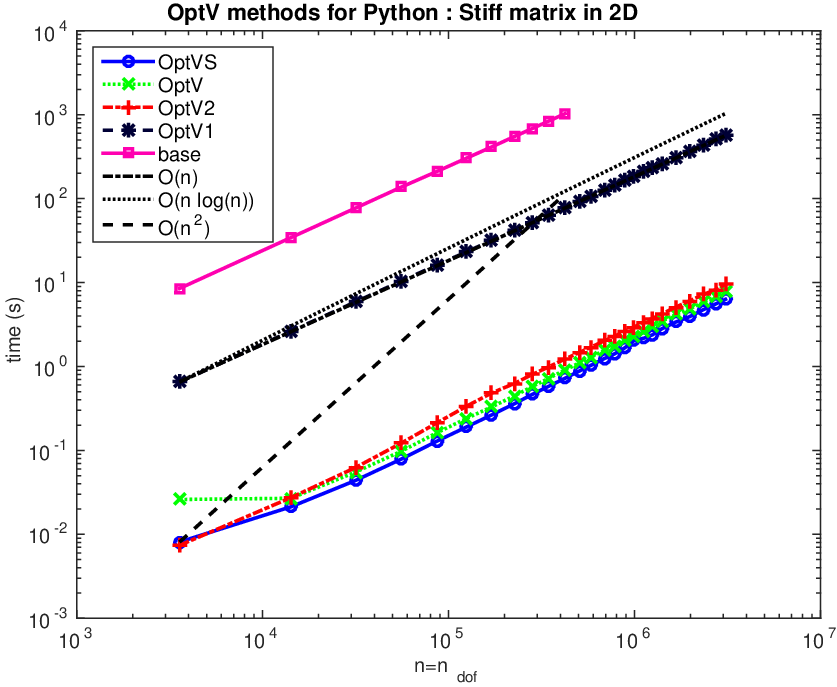
We show in Figures 4 and 5, in logarithmic scales and for each vector language, the performance of the assembly codes versus the matrix dimension ndof,{\mathop{\rm n_{dof}}\nolimits}, for the 2D stiffness and 3D elastic stiffness matrices respectively. We observe that the OptVS version is the fastest one and its complexity is 𝒪⁡(ndof)\mathcal{O}\left({{\mathop{\rm n_{dof}}\nolimits}}\right).

Refer to captionRefer to captionRefer to caption
Figure 4: Stiffness matrix (2D): comparison of base, OptV1, OptV2, OptV and OptVS codes in Matlab (top left), Octave (top right) and Python (bottom).
Refer to captionRefer to captionRefer to caption
Figure 5: Elastic stiffness matrix (3D): comparison of base, OptV1, OptV2, OptV and OptVS codes in Matlab (top left), Octave (top right) and Python (bottom).

For the stiffness matrix in 2D, the OptV1 version is about 4040, 9595 and 550550 times slower in Matlab, Python and Octave respectively. Its numerical complexity is 𝒪⁡(ndof)\mathcal{O}\left({{\mathop{\rm n_{dof}}\nolimits}}\right). The complexity of the less performing method, the base version, is 𝒪⁡(ndof2)\mathcal{O}\left({{\mathop{\rm n^{2}_{dof}}\nolimits}}\right) in Matlab and Octave, while it seems to be 𝒪⁡(ndof)\mathcal{O}\left({{\mathop{\rm n_{dof}}\nolimits}}\right) in Python. This is partly due to the use of the LIL format in the sparse matrix assembly in Python, the conversion to the CSC format being included in the computation time. We obtain similar results for the stiffness matrix in 3D and the elastic stiffness matrices in 2D and 3D. Computation times and OptVS speedup are given in Tables 2 and 3 for the 2D stiffness and 3D elastic stiffness matrices respectively. For the 3D stiffness and the 2D elastic stiffness matrices one can refer respectively to Tables 9 and 10. We observe that the performance differences of the stiffness and elastic stiffness matrix assemblies in 2D and 3D are partly due to the increase of the data: on the unit disk (2D) and the unit sphere (3D), we have nme≈2nq{\mathop{\rm n_{me}}\nolimits}\approx 2{\mathop{\rm n_{q}}\nolimits} and nme≈6nq{\mathop{\rm n_{me}}\nolimits}\approx 6{\mathop{\rm n_{q}}\nolimits} respectively. For matrices of the same size (i.e. for an equal ndof{\mathop{\rm n_{dof}}\nolimits}), in comparison to the 2D stiffness matrix, the number of local values to be computed are 2, 4 and 16 times larger for the 2D elastic stiffness, the 3D stiffness and the 3D elastic stiffness matrices respectively.

StiffAssembling2DP1 - Matlab StiffAssembling2DP1 - Octave nd​o​fn_{dof} OptVS OptV OptV2 OptV1 base 1422214222 .063 (s) x 1 .044 (s) x .692 .053 (s) x .833 1.70 (s) x 26.8 6.79 (s) x 107 125010125010 .411 (s) x 1 .617 (s) x 1.5 .553 (s) x 1.35 14.4 (s) x 35.1 226 (s) x 550 343082343082 .985 (s) x 1 1.37 (s) x 1.39 1.36 (s) x 1.38 39.1 (s) x 39.7 1873 (s) x 1902 885521885521 2.34 (s) x 1 3.24 (s) x 1.39 3.29 (s) x 1.41 99.7 (s) x 42.7 - 19786021978602 5.45 (s) x 1 7.60 (s) x 1.40 7.28 (s) x 1.34 223 (s) x 40.9 - nd​o​fn_{dof} OptVS OptV OptV2 OptV1 base 1422214222 .017 (s) x 1 .058 (s) x 3.36 .036 (s) x 2.09 14.3 (s) x 826 15.4 (s) x 888 125010125010 .167 (s) x 1 .218 (s) x 1.31 .221 (s) x 1.33 124 (s) x 742 255 (s) x 1533 343082343082 .499 (s) x 1 .656 (s) x 1.32 .835 (s) x 1.67 340 (s) x 681 1458 (s) x 2923 885521885521 1.47 (s) x 1 1.91 (s) x 1.30 2.43 (s) x 1.65 899 (s) x 613 - 19786021978602 3.64 (s) x 1 4.63 (s) x 1.27 5.44 (s) x 1.49 2007 (s) x 551 - StiffAssembling2DP1 - Python nd​o​fn_{dof} OptVS OptV OptV2 OptV1 base 1422214222 .021 (s) x 1 .027 (s) x 1.26 .027 (s) x 1.29 2.64 (s) x 124 34.4 (s) x 1614 125010125010 .190 (s) x 1 .241 (s) x 1.26 .336 (s) x 1.77 23.2 (s) x 122 303 (s) x 1594 343082343082 .576 (s) x 1 .716 (s) x 1.24 .980 (s) x 1.70 63.5 (s) x 110 833 (s) x 1445 885521885521 1.66 (s) x 1 2.05 (s) x 1.23 2.62 (s) x 1.58 164 (s) x 98.9 - 19786021978602 3.92 (s) x 1 4.85 (s) x 1.24 6.04 (s) x 1.54 368 (s) x 93.9 -

Table 2: Stiffness matrix (2D) : comparison of OptVS, OptV, OptV1 and base codes in Matlab (top left), Octave (top right) and Python (bottom) giving time in seconds (top value) and OptVS speedup (bottom value).

StiffElasAssembling3DP1 - Matlab StiffElasAssembling3DP1 - Octave nd​o​fn_{dof} OptVS OptV OptV2 OptV1 base 1677316773 .560 (s) x 1 .971 (s) x 1.73 .924 (s) x 1.65 67.6 (s) x 121 236 (s) x 422 4412444124 1.70 (s) x 1 3.45 (s) x 2.03 2.60 (s) x 1.52 184 (s) x 108 1427 (s) x 837 121710121710 4.43 (s) x 1 8.12 (s) x 1.83 7.55 (s) x 1.70 540 (s) x 122 1E+4 (s) x 2716 601272601272 27.5 (s) x 1 47.4 (s) x 1.72 41.5 (s) x 1.51 2765 (s) x 101 - 11446801144680 51.5 (s) x 1 89.4 (s) x 1.74 84.2 (s) x 1.64 5254 (s) x 102 - nd​o​fn_{dof} OptVS OptV OptV2 OptV1 base 1677316773 .364 (s) x 1 .628 (s) x 1.73 .569 (s) x 1.56 255 (s) x 701 321 (s) x 882 4412444124 .993 (s) x 1 1.69 (s) x 1.71 1.49 (s) x 1.50 698 (s) x 703 1314 (s) x 1323 121710121710 3.03 (s) x 1 5.13 (s) x 1.69 4.19 (s) x 1.38 1976 (s) x 651 9338 (s) x 3078 601272601272 18.9 (s) x 1 31.7 (s) x 1.68 25.5 (s) x 1.35 9853 (s) x 521 - 11446801144680 40.9 (s) x 1 69.1 (s) x 1.69 55.6 (s) x 1.36 2E+4 (s) x 471 - StiffElasAssembling3DP1 - Python nd​o​fn_{dof} OptVS OptV OptV2 OptV1 base 1677316773 .391 (s) x 1 .622 (s) x 1.59 .486 (s) x 1.24 122 (s) x 312 784 (s) x 2004 4412444124 .954 (s) x 1 1.56 (s) x 1.63 1.32 (s) x 1.38 333 (s) x 349 2141 (s) x 2243 121710121710 2.55 (s) x 1 4.21 (s) x 1.65 3.79 (s) x 1.49 946 (s) x 372 6071 (s) x 2384 601272601272 16.4 (s) x 1 27.6 (s) x 1.68 24.9 (s) x 1.52 4850 (s) x 296 - 11446801144680 36.4 (s) x 1 61.5 (s) x 1.69 54.2 (s) x 1.49 - -

Table 3: Elastic stiffness matrix (3D) : comparison of OptVS, OptV, OptV2, OptV1 and base codes in Matlab (top left), Octave (top right) and Python (bottom) giving time in seconds (top value) and OptVS speedup (bottom value).

In Figure 6 we compare the maximum of memory for OptVS, OptV and OptV2 codes. The OptV2 method is more consuming than OptVS and OptV respectively by a factor between 5 and 6.3 and between 6 and 8.9 depending on the language.

Refer to caption
Figure 6: Elastic stiffness matrix (3D): memory usage in MB and ratio between the slope of each method and OptV in Python (in the caption)

6.2 Comparison of the OptVS version with CXSparse and FreeFEM++

In Tables 4 the OptVS codes in Matlab/Octave/Python are compared with a C implementation of the assembly (OptV1 version) using the SuiteSparse library [10] (“CXSparse”) and with a FreeFEM++ code for the stiffness matrix in 2D and the elastic stiffness matrix in 3D.

The computation cost for the stiffness matrix in 3D and the elastic stiffness matrix in 2D are given in Tables 7 and 8. We observe that OptVS version is approximately 1.5 and 5.5 times in Matlab, 2 and 7.5 times in Octave, and 2.1 and 8.5 times in Python faster than FreeFEM++. Compared to C, computation times are multiplied by a factor between 2.5 and 4.7 in Matlab, 1.9 and 3.7 in Octave, and 1.8 and 3.2 in Python. Unlike what is commonly believed the performance is not radically worse than that of C.

nd​o​fn_{dof} CXSparse (4.2.1) Matlab (2014b) Octave (3.8.1) Python (3.4.0) FreeFEM (3.31) 1422214222 0.014 (s) x 1.00 0.063 (s) x 4.64 0.017 (s) x 1.26 0.021 (s) x 1.56 0.071 (s) x 5.16 125010125010 0.073 (s) x 1.00 0.411 (s) x 5.62 0.167 (s) x 2.28 0.190 (s) x 2.60 0.501 (s) x 6.85 343082343082 0.221 (s) x 1.00 0.985 (s) x 4.46 0.499 (s) x 2.26 0.576 (s) x 2.61 1.421 (s) x 6.43 885521885521 0.606 (s) x 1.00 2.337 (s) x 3.86 1.467 (s) x 2.42 1.660 (s) x 2.74 3.692 (s) x 6.10 19786021978602 1.354 (s) x 1.00 5.446 (s) x 4.02 3.644 (s) x 2.69 3.920 (s) x 2.89 8.305 (s) x 6.13

nd​o​fn_{dof} CXSparse (4.2.1) Matlab (2014b) Octave (3.8.1) Python (3.4.0) FreeFEM (3.31) 1677316773 0.137 (s) x 1.00 0.560 (s) x 4.09 0.364 (s) x 2.66 0.391 (s) x 2.86 3.827 (s) x 27.95 4412444124 0.398 (s) x 1.00 1.705 (s) x 4.29 0.993 (s) x 2.50 0.954 (s) x 2.40 10.440 (s) x 26.26 121710121710 1.193 (s) x 1.00 4.433 (s) x 3.72 3.034 (s) x 2.54 2.547 (s) x 2.13 29.914 (s) x 25.08 601272601272 6.386 (s) x 1.00 27.482 (s) x 4.30 18.894 (s) x 2.96 16.359 (s) x 2.56 152.553 (s) x 23.89 11446801144680 12.477 (s) x 1.00 51.465 (s) x 4.12 40.940 (s) x 3.28 36.392 (s) x 2.92 293.307 (s) x 23.51

Table 4: 2D Stiffness matrix (top table) and 3D elastic stiffness matrix (bottom table) : computational cost versus nd​o​f,n_{dof}, with the OptVS Matlab/Octave/Python version (2nd/3rd/4th2^{\mbox{nd}}/3^{\mbox{rd}}/4^{\mbox{th}} columns), with CXSparse (1st1^{\mbox{st}} column) and FreeFEM++ (5th5^{\mbox{th}} column); time in seconds (top value) and CXSparse speedup (bottom value).

6.3 Comparison with other matrix assemblies in Matlab and Octave

In Matlab/Octave other efficient algorithms have been proposed recently in [2, 3, 17, 34]. More precisely, in [17], a vectorization is proposed, based on the permutation of two local loops with the one through the elements. This technique allows to easily assemble different matrices, from a reference element by affine transformation and by using a numerical integration. In [34], the implementation is based on extending element operations on arrays into operations on arrays of matrices, calling them matrix-array operations. The array elements are matrices instead of scalars and the operations are defined by the rules of linear algebra. Thanks to these new tools and a quadrature formula, different matrices are computed without any loop. In [3], for the assembly of the stiffness matrix in 2D associated to ℙ1{\mathbb{P}_{1}} finite elements, L. Chen constructs vectorially the nine sparse matrices corresponding to the nine elements of the local stiffness matrix in 2D and adds them to obtain the global matrix. The restriction to d=2d=2 or 33 of Algorithm 4.2 corresponds to the method in [3].

We compare these codes to OptVS for the assembly of the stiffness matrix in 2D. In Tables 5 and 6, using Matlab and Octave respectively, computation times versus the number of vertices are given for the different codes. OptVS speedup is between 11 and 2.52.5 in comparison with the other vectorized codes for sufficiently fine meshes.

nd​o​fn_{dof} OptVs Chen iFEM HanJun RahVal 125010125010 0.411 (s) x 1.00 0.616 (s) x 1.50 0.693 (s) x 1.69 0.646 (s) x 1.57 0.664 (s) x 1.61 343082343082 0.985 (s) x 1.00 1.464 (s) x 1.49 1.257 (s) x 1.28 1.989 (s) x 2.02 2.096 (s) x 2.13 885521885521 2.337 (s) x 1.00 3.307 (s) x 1.41 2.966 (s) x 1.27 4.372 (s) x 1.87 4.721 (s) x 2.02 19786021978602 5.446 (s) x 1.00 9.286 (s) x 1.71 7.221 (s) x 1.33 9.813 (s) x 1.80 9.123 (s) x 1.68 30856283085628 8.644 (s) x 1.00 12.332 (s) x 1.43 11.444 (s) x 1.32 14.562 (s) x 1.68 14.841 (s) x 1.72

Table 5: Stiffness matrix (2D): computational cost in Matlab (R2014b) versus nq,{\mathop{\rm n_{q}}\nolimits}, with the OptVS version (column 22) and with the codes in [2, 3, 17, 34] (columns 33-66) : time in seconds (top value) and speedup (bottom value). The speedup reference is OptVS version.

nd​o​fn_{dof} OptVs Chen iFEM HanJun RahVal 125010125010 0.167 (s) x 1.00 0.305 (s) x 1.83 0.288 (s) x 1.73 0.417 (s) x 2.50 0.486 (s) x 2.92 343082343082 0.499 (s) x 1.00 0.823 (s) x 1.65 0.644 (s) x 1.29 1.299 (s) x 2.60 1.245 (s) x 2.50 885521885521 1.467 (s) x 1.00 2.123 (s) x 1.45 1.663 (s) x 1.13 3.720 (s) x 2.54 3.221 (s) x 2.20 19786021978602 3.644 (s) x 1.00 4.674 (s) x 1.28 3.832 (s) x 1.05 8.279 (s) x 2.27 7.164 (s) x 1.97 30856283085628 6.457 (s) x 1.00 7.786 (s) x 1.21 6.642 (s) x 1.03 13.523 (s) x 2.09 11.583 (s) x 1.79

Table 6: Stiffness matrix (2D): computational cost in Octave (3.8.1) versus nq,{\mathop{\rm n_{q}}\nolimits}, with the OptVS version (column 22) and with the codes in [2, 3, 17, 34] (columns 33-66) : time in seconds (top value) and speedup (bottom value). The speedup reference is OptVS version.

In Figure 7 we compare the memory costs in Matlab of our assembly codes with the other ones. As expected the consumption of OptVS and OptV methods are observed to be close to that of iFEM and lower than that of the other codes.

Refer to caption
Figure 7: Stiffness matrix (2D): memory usage in MB and ratio between the slope of each method and OptVS (in the caption)

7 Conclusion and work in progress

We presented vectorized algorithms for the assembly of ℙ1{\mathbb{P}_{1}} finite element matrices in arbitrary dimension. The implementation of these algorithms has been done in different vector languages such as Matlab, Octave and Python to calculate the stiffness and elastic stiffness matrices. Computation times of different versions (vectorized or not) have been compared in several interpreted languages and C. Numerical examples show the efficiency of the OptV2, OptV and OptVS algorithms. More precisely, for the OptVS method, the assembly of the stiffness matrix in 2D of size 10610^{6} is performed in 2.62.6, 1.751.75 and 22 seconds with Matlab, Octave and Python respectively and in 0.750.75 seconds with C. Less performance is obtained for the assembly of the elastic stiffness matrix in 3D: a matrix of size 10610^{6} is computed in 4545, 35.835.8 and 31.831.8 seconds, with Matlab, Octave and Python respectively and in 10.910.9 seconds with C. Moreover we observed that OptVS is about 1.4 times faster than the non-symmetrized versions OptV and OptV2. OptV and OptVS methods are less memory consuming than OptV2. Preliminary results towards the extension to ℙk{\mathbb{P}_{k}} finite elements are given in the Appendix. The algorithms in arbitrary dimension for piecewise polynomials of higher order, is the subject of a future paper. The OptV2 algorithm has been also implemented with a NVIDIA GPU33 3 GeForce GTX Titan Black, 2880 CUDA Core, 6Go Memory, using the Thrust and Cusp libraries. For the 2D elastic stiffness and 3D stiffness matrices, the OptV2 code is respectively 3.5 and 7 times faster on GPU than the C code (the time for GPU/CPU data and matrix transfers is taken into account).

Vectorization gave good performance and the vectorized code can be used for other matrices or discretizations, the only part of the code that have to be reviewed (which is probably the most difficult part) is the vectorization of the element matrix computation. We have seen that it is possible to efficiently assemble matrices of large size in interpreted languages. In this framework Python showed some very good performance even though Octave seems to be more efficient in some cases. Moreover the performance of our vectorized codes was better in Octave than in Matlab. The Python and Matlab/Octave codes are available online (see [7]).

Appendix A Additional benchmark results

In this section, we consider the assembly of the 3D stiffness and 2D elastic stiffness matrices. In Tables 7 and 8 we compare the OptVS versions in Matlab/Octave/Python with a C implementation of the assembly (OptV1 version) using the SuiteSparse library [10] (“CXSparse”), and with a FreeFEM++ version. In Tables 9 and 10 the computation times of OptVS, OptV, OptV2, OptV1 and base versions are compared in Matlab, Octave and Python. We observe similar results as in Section 6.

nd​o​fn_{dof} CXSparse (4.2.1) Matlab (2014b) Octave (3.8.1) Python (3.4.0) FreeFEM (3.31) 1470814708 0.087 (s) x 1.00 0.135 (s) x 1.55 0.143 (s) x 1.64 0.191 (s) x 2.19 0.545 (s) x 6.26 4057040570 0.155 (s) x 1.00 0.461 (s) x 2.97 0.293 (s) x 1.89 0.377 (s) x 2.43 1.571 (s) x 10.12 200424200424 1.014 (s) x 1.00 3.457 (s) x 3.41 1.911 (s) x 1.88 1.935 (s) x 1.91 8.742 (s) x 8.62 580975580975 3.844 (s) x 1.00 9.767 (s) x 2.54 7.193 (s) x 1.87 6.804 (s) x 1.77 26.970 (s) x 7.02 17478611747861 10.752 (s) x 1.00 31.203 (s) x 2.90 31.008 (s) x 2.88 26.069 (s) x 2.42 84.698 (s) x 7.88

Table 7: Stiffness matrix (3D) : computational cost versus nd​o​f,n_{dof}, with the OptVS Matlab/Octave/Python version (2nd/3rd/4th2^{\mbox{nd}}/3^{\mbox{rd}}/4^{\mbox{th}} columns), with CXSparse (1st1^{\mbox{st}} column) and FreeFEM++ (5th5^{\mbox{th}} column) : time in seconds (top value) and speedup (bottom value). The speedup reference is CXSparse code.

nd​o​fn_{dof} CXSparse (4.2.1) Matlab (2014b) Octave (3.8.1) Python (3.4.0) FreeFEM (3.31) 2844428444 0.023 (s) x 1.00 0.139 (s) x 5.92 0.115 (s) x 4.88 0.076 (s) x 3.25 0.762 (s) x 32.47 111838111838 0.107 (s) x 1.00 0.412 (s) x 3.84 0.321 (s) x 2.99 0.288 (s) x 2.69 2.865 (s) x 26.75 250020250020 0.267 (s) x 1.00 1.046 (s) x 3.92 0.727 (s) x 2.73 0.662 (s) x 2.48 6.432 (s) x 24.11 10134121013412 1.133 (s) x 1.00 5.000 (s) x 4.41 4.238 (s) x 3.74 3.377 (s) x 2.98 26.301 (s) x 23.20 28022582802258 3.142 (s) x 1.00 14.867 (s) x 4.73 11.483 (s) x 3.65 10.036 (s) x 3.19 72.561 (s) x 23.10

Table 8: Elastic stiffness matrix (2D) : computational cost versus nd​o​f,n_{dof}, with the OptVS Matlab/Octave/Python version (2nd/3rd/4th2^{\mbox{nd}}/3^{\mbox{rd}}/4^{\mbox{th}} columns), with CXSparse (1st1^{\mbox{st}} column) and FreeFEM++ (5th5^{\mbox{th}} column) : time in seconds (top value) and speedup (bottom value). The speedup reference is CXSparse code.

StiffAssembling3DP1 - Matlab StiffAssembling3DP1 - Octave nd​o​fn_{dof} OptVS OptV OptV2 OptV1 base 1470814708 .135 (s) x 1 .409 (s) x 3.03 .442 (s) x 3.27 5.07 (s) x 37.5 25.6 (s) x 189 4057040570 .461 (s) x 1 .827 (s) x 1.80 .775 (s) x 1.68 14.0 (s) x 30.3 112 (s) x 244 200424200424 3.46 (s) x 1 4.69 (s) x 1.36 4.74 (s) x 1.37 69.6 (s) x 20.1 3255 (s) x 942 580975580975 9.77 (s) x 1 13.2 (s) x 1.35 14.1 (s) x 1.44 204 (s) x 20.9 - 17478611747861 31.2 (s) x 1 40.4 (s) x 1.29 44.5 (s) x 1.42 623 (s) x 20.0 - nd​o​fn_{dof} OptVS OptV OptV2 OptV1 base 1470814708 .143 (s) x 1 .177 (s) x 1.24 .146 (s) x 1.02 76.0 (s) x 531 77.3 (s) x 540 4057040570 .293 (s) x 1 .446 (s) x 1.52 .488 (s) x 1.66 216 (s) x 737 248 (s) x 844 200424200424 1.91 (s) x 1 2.37 (s) x 1.24 3.15 (s) x 1.65 1120 (s) x 586 3041 (s) x 1592 580975580975 7.19 (s) x 1 9.15 (s) x 1.27 10.6 (s) x 1.47 3264 (s) x 454 - 17478611747861 31.0 (s) x 1 38.0 (s) x 1.22 40.5 (s) x 1.31 - - StiffAssembling3DP1 - Python nd​o​fn_{dof} OptVS OptV OptV2 OptV1 base 1470814708 .191 (s) x 1 .207 (s) x 1.08 .258 (s) x 1.35 12.8 (s) x 67.0 172 (s) x 903 4057040570 .377 (s) x 1 .530 (s) x 1.41 .823 (s) x 2.19 36.0 (s) x 95.5 488 (s) x 1295 200424200424 1.93 (s) x 1 2.50 (s) x 1.29 4.15 (s) x 2.14 182 (s) x 94.0 2480 (s) x 1282 580975580975 6.80 (s) x 1 8.89 (s) x 1.31 12.4 (s) x 1.83 541 (s) x 79.5 - 17478611747861 26.1 (s) x 1 34.2 (s) x 1.31 40.3 (s) x 1.55 - -

Table 9: Stiffness matrix (3D) : comparison of OptVS, OptV, OptV2, OptV1 and base codes in Matlab (top left), Octave (top right) and Python (bottom) giving time in seconds (top value) and OptVS speedup (bottom value).

StiffElasAssembling2DP1 - Matlab StiffElasAssembling2DP1 - Octave nd​o​fn_{dof} OptVS OptV OptV2 OptV1 base 2844428444 .114 (s) x 1 .272 (s) x 2.39 .185 (s) x 1.63 16.9 (s) x 148 67.8 (s) x 594 250020250020 1.01 (s) x 1 1.68 (s) x 1.65 1.91 (s) x 1.88 150 (s) x 148 6156 (s) x 6073 686164686164 3.20 (s) x 1 5.28 (s) x 1.65 5.42 (s) x 1.70 414 (s) x 129 - 17710421771042 8.97 (s) x 1 14.7 (s) x 1.64 15.2 (s) x 1.69 1090 (s) x 122 - 39572043957204 21.6 (s) x 1 34.1 (s) x 1.58 33.1 (s) x 1.53 - - nd​o​fn_{dof} OptVS OptV OptV2 OptV1 base 2844428444 .082 (s) x 1 .129 (s) x 1.57 .091 (s) x 1.11 63.7 (s) x 777 88.6 (s) x 1080 250020250020 .726 (s) x 1 1.26 (s) x 1.74 .915 (s) x 1.26 564 (s) x 777 4485 (s) x 6176 686164686164 2.21 (s) x 1 3.57 (s) x 1.61 3.36 (s) x 1.52 1550 (s) x 701 - 17710421771042 6.85 (s) x 1 10.7 (s) x 1.56 9.39 (s) x 1.37 - - 39572043957204 16.2 (s) x 1 25.8 (s) x 1.59 22.0 (s) x 1.36 - - StiffElasAssembling2DP1 - Python nd​o​fn_{dof} OptVS OptV OptV2 OptV1 base 2844428444 .136 (s) x 1 .207 (s) x 1.53 .202 (s) x 1.49 30.0 (s) x 221 183 (s) x 1348 250020250020 .721 (s) x 1 1.08 (s) x 1.50 1.22 (s) x 1.7 277 (s) x 384 1639 (s) x 2274 686164686164 2.05 (s) x 1 3.06 (s) x 1.50 3.55 (s) x 1.73 761 (s) x 372 - 17710421771042 6.06 (s) x 1 9.12 (s) x 1.50 9.58 (s) x 1.58 - - 39572043957204 14.0 (s) x 1 21.2 (s) x 1.52 21.5 (s) x 1.54 - -

Table 10: Elastic stiffness matrix (2D): comparison of OptVS, OptV, OptV2 , OptV1 and base codes in Matlab (top left), Octave (top right) and Python (bottom) giving time in seconds (top value) and OptVS speedup (bottom value).

Appendix B Proof of Lemma 1

To prove Lemma 1, we introduce the following matrix 𝔹l\mathbb{B}_{l} :

𝔹l=(δl,100δl,2δl,2δl,1)if​d=2,and𝔹l=(δl,1000δl,2000δl,3δl,2δl,100δl,3δl,2δl,30δl,1)if​d=3.\mathbb{B}_{l}=\begin{pmatrix}\delta_{l,1}&0\\ 0&\delta_{l,2}\\ \delta_{l,2}&\delta_{l,1}\end{pmatrix}\ \ \mbox{if}\ d=2,\ \ \mbox{and}\ \ \mathbb{B}_{l}=\begin{pmatrix}\delta_{l,1}&0&0\\ 0&\delta_{l,2}&0\\ 0&0&\delta_{l,3}\\ \delta_{l,2}&\delta_{l,1}&0\\ 0&\delta_{l,3}&\delta_{l,2}\\ \delta_{l,3}&0&\delta_{l,1}\end{pmatrix}\ \ \mbox{if}\ d=3.

Thus we have ϵ¯​(𝝀l,α)=𝔹l​∇λα\underline{\boldsymbol{\epsilon}}(\boldsymbol{\lambda}_{l,{\rm\alpha}})=\mathbb{B}_{l}\mathop{\rm\nabla}\nolimits\lambda_{\rm\alpha} and then

ϵ¯t​(𝝀n,β)​ℂ​ϵ¯​(𝝀l,α)=∇λβt​𝔹nt​ℂ​𝔹l​∇λα.\underline{\boldsymbol{\epsilon}}^{t}(\boldsymbol{\lambda}_{n,{\rm\beta}})\mathbb{C}\underline{\boldsymbol{\epsilon}}(\boldsymbol{\lambda}_{l,{\rm\alpha}})=\mathop{\rm\nabla}\nolimits\lambda_{\rm\beta}^{t}\mathbb{B}_{n}^{t}\mathbb{C}\mathbb{B}_{l}\mathop{\rm\nabla}\nolimits\lambda_{\rm\alpha}.

Moreover we have ℂ=λ​ℂ0+μ​ℂ1\mathbb{C}=\lambda\mathbb{C}_{0}+\mu\mathbb{C}_{1} with

ℂ0=(𝟙d𝕆d,2​d−3𝕆2​d−3,d𝕆2​d−3)3​(d−1)×3​(d−1)andℂ1=(2​𝕀d𝕆d,2​d−3𝕆2​d−3,d𝕀2​d−3)3​(d−1)×3​(d−1)\mathbb{C}_{0}=\begin{pmatrix}\mathds{1}_{d}&\mathds{O}_{d,2d-3}\\ \mathds{O}_{2d-3,d}&\mathds{O}_{2d-3}\end{pmatrix}_{3(d-1)\times 3(d-1)}\ \ \mbox{and}\ \ \mathbb{C}_{1}=\begin{pmatrix}2\mathbb{I}_{d}&\mathds{O}_{d,2d-3}\\ \mathds{O}_{2d-3,d}&\mathbb{I}_{2d-3}\end{pmatrix}_{3(d-1)\times 3(d-1)}

Thus we obtain

ϵ¯t​(𝝀n,β)​ℂ​ϵ¯​(𝝀l,α)=λ​∇λβt​𝔹nt​ℂ0​𝔹l​∇λα+μ​∇λβt​𝔹nt​ℂ1​𝔹l​∇λα.\underline{\boldsymbol{\epsilon}}^{t}(\boldsymbol{\lambda}_{n,{\rm\beta}})\mathbb{C}\underline{\boldsymbol{\epsilon}}(\boldsymbol{\lambda}_{l,{\rm\alpha}})=\lambda\mathop{\rm\nabla}\nolimits\lambda_{\rm\beta}^{t}\mathbb{B}_{n}^{t}\mathbb{C}_{0}\mathbb{B}_{l}\mathop{\rm\nabla}\nolimits\lambda_{\rm\alpha}+\mu\mathop{\rm\nabla}\nolimits\lambda_{\rm\beta}^{t}\mathbb{B}_{n}^{t}\mathbb{C}_{1}\mathbb{B}_{l}\mathop{\rm\nabla}\nolimits\lambda_{\rm\alpha}.

Denoting ℚn,l=𝔹nt​ℂ0​𝔹l\mathbb{Q}^{n,l}=\mathbb{B}_{n}^{t}\mathbb{C}_{0}\mathbb{B}_{l} and 𝕊n,l=𝔹nt​ℂ1​𝔹l\mathbb{S}^{n,l}=\mathbb{B}_{n}^{t}\mathbb{C}_{1}\mathbb{B}_{l} we obtain (15) which ends the proof of Lemma 1.

Appendix C Remaining routines

C.1 Gradients of the barycentric coordinates

Let TkT_{k} be a dd-simplex of ℝd\mathbb{R}^{d} with vertices q0,…,qd{\rm q}^{0},\ldots,{\rm q}^{d}, and T^\hat{T} be the reference dd-simplex with vertices q^0,…,q^d\hat{{\rm q}}^{0},\ldots,\hat{{\rm q}}^{d} where q^0=𝟎d\hat{{\rm q}}^{0}=\boldsymbol{0}_{d} and q^i=𝒆i,\hat{{\rm q}}^{i}=\boldsymbol{e}_{i}, ∀i∈{1,…,d}.\forall i\in\left\{{{1},\ldots,{d}}\right\}.

Let ℱk\mathcal{F}_{k} be the bijection from T^\hat{T} to TkT_{k} defined by q=ℱk​(q^)=𝔹k​q^+q0{\rm q}=\mathcal{F}_{k}(\hat{{\rm q}})=\mathbb{B}_{k}\hat{{\rm q}}+{\rm q}^{0} where 𝔹k∈ℳd​(ℝ)\mathbb{B}_{k}\in\mathcal{M}_{d}(\mathbb{R}) is such that its ii-th column is equal to qi−q0,{\rm q}^{i}-{\rm q}^{0}, for all i∈{1,…,d}.i\in\left\{{{1},\ldots,{d}}\right\}.

The barycentric coordinates of q^=(x^1,…,x^d)∈T^\hat{{\rm q}}=(\hat{x}_{1},\ldots,\hat{x}_{d})\in\hat{T} are given by λ^0=1−∑i=1dx^i,\hat{\lambda}_{0}=1-\sum_{i=1}^{d}\hat{x}_{i}, and λ^i=x^i,\hat{\lambda}_{i}=\hat{x}_{i}, ∀i∈{1,…,d}.\forall i\in\left\{{{1},\ldots,{d}}\right\}. The barycentric coordinates of q=(x1,…,xd)∈Tk{\rm q}=(x_{1},\ldots,x_{d})\in T_{k} are given by λk,i​(q)=λ^i∘ℱk−1​(q)\lambda_{k,i}({\rm q})=\hat{\lambda}_{i}\circ\mathcal{F}^{-1}_{k}({\rm q}) and we have

∇λk,i​(q)=𝔹k−t​∇^​λ^i​(q^),∀i∈{0,…,d},\mathop{\rm\nabla}\nolimits\lambda_{k,i}({\rm q})=\mathbb{B}_{k}^{-t}\hat{\mathop{\rm\nabla}\nolimits}\hat{\lambda}_{i}(\hat{{\rm q}}),\ \forall i\in\left\{{{0},\ldots,{d}}\right\}, (17)

with ∇^​λ^0​(q^)=(−1…−1),\hat{\mathop{\rm\nabla}\nolimits}\hat{\lambda}_{0}(\hat{{\rm q}})=\begin{pmatrix}-1\\ \ldots\\ -1\end{pmatrix}, ∇^​λ^i=𝒆i,\hat{\mathop{\rm\nabla}\nolimits}\hat{\lambda}_{i}=\boldsymbol{e}_{i}, ∀i∈{1,…,d}.\forall i\in\left\{{{1},\ldots,{d}}\right\}. Note that gradients are constant. Let

𝔾^=(∇^​λ^0,…,∇^​λ^d)=(−110…0−101⋱⋱⋱0−10…01).\hat{\mathbb{G}}=\begin{pmatrix}\hat{\mathop{\rm\nabla}\nolimits}\hat{\lambda}_{0},&\ldots,&\hat{\mathop{\rm\nabla}\nolimits}\hat{\lambda}_{d}\end{pmatrix}=\begin{pmatrix}-1&1&0&\ldots&0\\ -1&0&1&\ddots&\vdots\\ \vdots&\vdots&\ddots&\ddots&0\\ -1&0&\ldots&0&1\end{pmatrix}.

Then computing the gradients of the barycentric coordinates is equivalent to solve (d+1)(d+1) linear systems, written in matrix form as follows:

𝔹kt​𝔾k=𝔾^,\mathbb{B}_{k}^{t}\mathbb{G}_{k}=\hat{\mathbb{G}}, (18)

where 𝔾k=(∇λk,0​(q),…,∇λk,d​(q))∈ℳd,d+1​(ℝ).\mathbb{G}_{k}=\begin{pmatrix}\mathop{\rm\nabla}\nolimits\lambda_{k,0}({\rm q}),&\ldots,&\mathop{\rm\nabla}\nolimits\lambda_{k,d}({\rm q})\end{pmatrix}\in\mathcal{M}_{d,d+1}(\mathbb{R}).

For each dd-simplex one has to calculate (d+1)(d+1) gradients and thus to determine (d+1)nme(d+1){\mathop{\rm n_{me}}\nolimits} vectors of dimension dd.

The vectorization of the calculation of the gradients is done by rewriting the equations (18), for k=1,…,nmek=1,...,{\mathop{\rm n_{me}}\nolimits}, under an equivalent form of a large block diagonal sparse system of size N=d×nmeN=d\times{\mathop{\rm n_{me}}\nolimits}, with dd-by-dd diagonal blocks given by:

(𝔹1t𝕆…𝕆𝕆⋱⋱⋱⋱𝕆𝕆…𝕆𝔹nmet)N×N​(𝔾1𝔾2𝔾nme)N×(d+1)=(𝔾^𝔾^𝔾^)N×(d+1)\begin{pmatrix}\mathbb{B}_{1}^{t}&\mathbb{O}&\ldots&\mathbb{O}\\ \mathbb{O}&\ddots&\ddots&\vdots\\ \vdots&\ddots&\ddots&\mathbb{O}\\ \mathbb{O}&\ldots&\mathbb{O}&\mathbb{B}_{{\mathop{\rm n_{me}}\nolimits}}^{t}\end{pmatrix}_{N\times N}\begin{pmatrix}\mathbb{G}_{1}\\ \mathbb{G}_{2}\\ \vdots\\ \mathbb{G}_{{\mathop{\rm n_{me}}\nolimits}}\\ \end{pmatrix}_{N\times(d+1)}=\begin{pmatrix}\hat{\mathbb{G}}\\ \hat{\mathbb{G}}\\ \vdots\\ \hat{\mathbb{G}}\\ \end{pmatrix}_{N\times(d+1)} (19)
Algorithm C.1 Vectorized computation of gradients of the basis functions in dimension dd
Function 𝑮←GradientVec\footnotesize\boldsymbol{G}\leftarrow{\footnotesize{\color[rgb]{1,0,0}\textsc{GradientVec}}}(q,me{\rm q},\mathop{\rm me}\nolimits)
 𝕂←𝕀←𝕁←zeros(d,d,nme)\mathbb{K}\leftarrow\mathbb{I}\leftarrow\mathbb{J}\leftarrow{\footnotesize{\color[rgb]{0,0,1}\textsc{zeros}}}(d,d,{\mathop{\rm n_{me}}\nolimits})
 ii←d∗[0:(nme−1)]{\texttt{ii}}\leftarrow d*[0:({\mathop{\rm n_{me}}\nolimits}-1)]
 for i←1i\leftarrow 1 to dd do
  for j←1j\leftarrow 1 to dd do
   𝕂(i,j,:)←q(i,me(j+1,:))−q(i,me(1,:))\mathbb{K}(i,j,:)\leftarrow{\rm q}(i,\mathop{\rm me}\nolimits(j+1,:))-{\rm q}(i,\mathop{\rm me}\nolimits(1,:))
   𝕀(i,j,:)←ii+j,𝕁(i,j,:)←ii+i\mathbb{I}(i,j,:)\leftarrow{\texttt{ii}}+j,\ \mathbb{J}(i,j,:)\leftarrow{\texttt{ii}}+i
  end for
 end for
 𝕊←sparse(𝕀(:),𝕁(:),𝕂(:),d∗nme,d∗nme)\mathbb{S}\leftarrow{\footnotesize{\color[rgb]{0,0,1}\textsc{sparse}}}(\mathbb{I}(:),\mathbb{J}(:),\mathbb{K}(:),d*{\mathop{\rm n_{me}}\nolimits},d*{\mathop{\rm n_{me}}\nolimits})
 ℝ←zeros(d∗nme,d+1)\mathbb{R}\leftarrow{\footnotesize{\color[rgb]{0,0,1}\textsc{zeros}}}(d*{\mathop{\rm n_{me}}\nolimits},d+1) ⊳\vartriangleright Build RHS
 𝔾^←[−𝟙d×1,𝕀d]\hat{\mathbb{G}}\leftarrow[-\mathds{1}_{d\times 1},\mathbb{I}_{d}]
 ℝ←copymat(𝔾^,nme,1)\mathbb{R}\leftarrow{\footnotesize{\color[rgb]{0,0,1}\textsc{copymat}}}(\hat{\mathbb{G}},{\mathop{\rm n_{me}}\nolimits},1)
 𝔾←solve​(𝕊,ℝ)\mathbb{G}\leftarrow{\footnotesize{\color[rgb]{0,0,1}\textsc{solve}}}(\mathbb{S},\mathbb{R}) ⊳\vartriangleright 𝔾(d(k−1)+i,α)=∂λα∂xi|Tk\mathbb{G}(d(k-1)+i,{\rm\alpha})=\frac{\partial\lambda_{\rm\alpha}}{\partial x_{i}}_{|T_{k}}
 𝔾←transform​(𝔾,…)\mathbb{G}\leftarrow{\footnotesize{\color[rgb]{0,0,1}\textsc{transform}}}(\mathbb{G},...) ⊳\vartriangleright such that 𝔾(k,α,i)=∂λα∂xi|Tk\mathbb{G}(k,{\rm\alpha},i)=\frac{\partial\lambda_{\rm\alpha}}{\partial x_{i}}_{|T_{k}}
end Function

The performance of this algorithm may be improved by writing specific algorithms in each dimension d=1,2d=1,2 or 33 (see Appendix A in [6]).

C.2 Elastic stiffness matrix assembly : algorithm using the symmetry

When the assembly matrix is symmetric, one may improve the performance of Algorithm 5.3 by using the symmetry of the element matrices (see Section 4), which leads to the following algorithm:

Algorithm C.2 (OptVS) - Optimized assembly in vector case (m>1m>1)
1: Function 𝕄←\mathbb{M}\leftarrow AssemblyVecGenP1OptVS(me,nq,…\mathop{\rm me}\nolimits,{\mathop{\rm n_{q}}\nolimits},\ldots)
2:  ndof←m∗nq{\mathop{\rm n_{dof}}\nolimits}\leftarrow m*{\mathop{\rm n_{q}}\nolimits}
3:  𝕄←𝕆ndof\mathbb{M}\leftarrow\mathbb{O}_{{\mathop{\rm n_{dof}}\nolimits}} ⊳\vartriangleright ndof{\mathop{\rm n_{dof}}\nolimits}-by-ndof{\mathop{\rm n_{dof}}\nolimits} sparse matrix
4:  for l←1l\leftarrow 1 to mm do
5:   for α←1{\rm\alpha}\leftarrow 1 to d+1d+1 do
6:    𝑰g←m∗(me(α,:)−1)+l\boldsymbol{I}_{g}\leftarrow m*(\mathop{\rm me}\nolimits({\rm\alpha},:)-1)+l
7:    i​i←m⁡(α−1)+lii\leftarrow m({\rm\alpha}-1)+l
8:    for n←1n\leftarrow 1 to mm do
9:      for β←1{\rm\beta}\leftarrow 1 to d+1d+1 do
10:       j​j←m⁡(β−1)+njj\leftarrow m({\rm\beta}-1)+n
11:       if i​i>j​jii>jj then
12:        𝑲g←vecHe​(l,α,n,β,…)\boldsymbol{K}_{g}\leftarrow{\footnotesize\color[rgb]{0.545,0,0}\textsc{vecHe}}(l,{\rm\alpha},n,{\rm\beta},\ldots)
13:        𝑱g←m∗(me(β,:)−1)+n\boldsymbol{J}_{g}\leftarrow m*(\mathop{\rm me}\nolimits({\rm\beta},:)-1)+n
14:        𝕄←𝕄+Sparse(𝑰g,𝑱g,𝑲g,ndof,ndof)\mathbb{M}\leftarrow\mathbb{M}+{\footnotesize{\color[rgb]{0,0,1}\textsc{Sparse}}}(\boldsymbol{I}_{g},\boldsymbol{J}_{g},\boldsymbol{K}_{g},{\mathop{\rm n_{dof}}\nolimits},{\mathop{\rm n_{dof}}\nolimits})
15:       end if
16:      end for
17:    end for
18:   end for
19:  end for
20:  𝕄←𝕄+𝕄′\mathbb{M}\leftarrow\mathbb{M}+\mathbb{M}^{\prime}
21:  for l←1l\leftarrow 1 to mm do
22:   for α←1{\rm\alpha}\leftarrow 1 to d+1d+1 do
23:    𝑰g←m∗(me(α,:)−1)+l\boldsymbol{I}_{g}\leftarrow m*(\mathop{\rm me}\nolimits({\rm\alpha},:)-1)+l
24:    𝑲g←vecHe​(l,α,l,α,…)\boldsymbol{K}_{g}\leftarrow{\footnotesize\color[rgb]{0.545,0,0}\textsc{vecHe}}(l,{\rm\alpha},l,{\rm\alpha},\ldots)
25:    𝕄←𝕄+Sparse(𝑰g,𝑰g,𝑲g,ndof,ndof)\mathbb{M}\leftarrow\mathbb{M}+{\footnotesize{\color[rgb]{0,0,1}\textsc{Sparse}}}(\boldsymbol{I}_{g},\boldsymbol{I}_{g},\boldsymbol{K}_{g},{\mathop{\rm n_{dof}}\nolimits},{\mathop{\rm n_{dof}}\nolimits})
26:   end for
27:  end for
28: end Function

Appendix D Extension to ℙk{\mathbb{P}_{k}}-Lagrange finite elements

In this section we adapt the optimized algorithm of Section 4 to the case of finite elements of higher order. For simplicity, we consider the assembly algorithm on the example of the mass matrix.

The mesh used is adapted to ℙk{\mathbb{P}_{k}} finite elements and is called a“ℙk{\mathbb{P}_{k}}-mesh”. Only arrays q{\rm q} and me\mathop{\rm me}\nolimits differ between the usual mesh and the ℙk{\mathbb{P}_{k}}-mesh. In the ℙk{\mathbb{P}_{k}}-mesh, q{\rm q} contains the coordinates of the nodal points associated to the ℙk{\mathbb{P}_{k}} finite elements and me\mathop{\rm me}\nolimits is of dimension ndfe{\mathop{\rm n_{dfe}}\nolimits}-by-nme{\mathop{\rm n_{me}}\nolimits}, where ndfe{\mathop{\rm n_{dfe}}\nolimits} is the local number of ℙk{\mathbb{P}_{k}}-nodes in a dd-simplex KK : ndfe=(d+k)!d!​k!{\mathop{\rm n_{dfe}}\nolimits}=\frac{(d+k)!}{d!k!}, as shown in the table below.

name type dimension description
ndfe{\mathop{\rm n_{dfe}}\nolimits} integer 1 local number of ℙk{\mathbb{P}_{k}}-nodes in a dd-simplex
nq{\mathop{\rm n_{q}}\nolimits} integer 1 number of ℙk{\mathbb{P}_{k}}-nodes
q{\rm q} double d×nq{\rm d}\times{\mathop{\rm n_{q}}\nolimits} array of ℙk{\mathbb{P}_{k}}-node coordinates
me\mathop{\rm me}\nolimits integer ndfe×nme{\mathop{\rm n_{dfe}}\nolimits}\times{\mathop{\rm n_{me}}\nolimits} (ℙk{\mathbb{P}_{k}}) connectivity array

By construction, the total number of degrees of freedom of a ℙk{\mathbb{P}_{k}}-mesh is its number of nodal points. One may use for example gmsh [16] to generate a ℙk{\mathbb{P}_{k}}-mesh in 2D or in 3D.

First, we need to introduce some notations: let 𝒮dk\mathcal{S}_{d}^{k} be the set of multi-indices given by

𝒮dk={𝜶=(α1,…,αd+1)∈ℕd+1such that|𝜶|:=∑i=1d+1αi=k},\mathcal{S}_{d}^{k}=\left\{\boldsymbol{\alpha}=(\alpha_{1},\ldots,\alpha_{d+1})\in\mathbb{N}^{d+1}\ \mbox{such that}\ |\boldsymbol{\alpha}|:=\sum_{i=1}^{d+1}\alpha_{i}=k\right\}, (20)

with #​𝒮d=N\#\mathcal{S}_{d}=N. Then the ℙk\mathbb{P}_{k} basis functions φ𝜶\varphi_{\boldsymbol{\alpha}} on a dd-simplex KK may be deduced from the barycentric coordinates {λj}j=1d+1\{\lambda_{j}\}_{j=1}^{d+1}

φ𝜶=∏l=1d+1∏j=0αl−1k​λl−jj+1,∀𝜶∈𝒮dk,\varphi_{\boldsymbol{\alpha}}=\prod_{l=1}^{d+1}\prod_{j=0}^{\alpha_{l}-1}\frac{k\lambda_{l}-j}{j+1},\ \ \ \forall\boldsymbol{\alpha}\in\mathcal{S}_{d}^{k}, (21)

or equivalently, noticing that φ𝜶\varphi_{\boldsymbol{\alpha}} is a polynomial in the variable (λ1,…,λd+1)(\lambda_{1},\ldots,\lambda_{d+1}) and introducing a multi-index 𝝁=(μ1,…,μd+1)∈ℕd+1\boldsymbol{\mu}=(\mu_{1},\ldots,\mu_{d+1})\in\mathbb{N}^{d+1}, we have

φ𝜶\displaystyle\varphi_{\boldsymbol{\alpha}} =∑|𝝁|≤ka𝝁​(𝜶)​(∏j=1d+1λjμj).\displaystyle=\sum_{|\boldsymbol{\mu}|\leq k}a_{\boldsymbol{\mu}}(\boldsymbol{\alpha})\left(\prod_{j=1}^{d+1}\lambda_{j}^{\mu_{j}}\right). (22)

All the non-zero a𝝁​(𝜶)a_{\boldsymbol{\mu}}(\boldsymbol{\alpha}) values can be computed from (21) and depend only on 𝜶,\boldsymbol{\alpha}, dd and kk.

As in the previous sections, the assembly algorithm of the mass matrix is based on the vectorization of the local mass matrix 𝕄e\mathbb{M}^{e} on KK, which is an NN-by-NN matrix given by

𝕄I⁡(𝜶),I⁡(𝜷)e​(K)=∫Kφ𝜶​φ𝜷​𝑑q,∀(𝜶,𝜷)∈𝒮dk×𝒮dk,\mathbb{M}_{I(\boldsymbol{\alpha}),I(\boldsymbol{\beta})}^{e}(K)=\int_{K}\varphi_{\boldsymbol{\alpha}}\varphi_{\boldsymbol{\beta}}d{\rm q},\ \ \forall(\boldsymbol{\alpha},\boldsymbol{\beta})\in\mathcal{S}_{d}^{k}\times\mathcal{S}_{d}^{k},

where I:𝒮dk⟶{1,…,N}{I}:{\mathcal{S}_{d}^{k}}\longrightarrow{\left\{{{1},\ldots,{N}}\right\}} is the local numbering choice.

We then introduce a formula of the same type as (8) to vectorize the computation of 𝕄e\mathbb{M}^{e}. Using (22), we have for all (𝜶,𝜷)∈𝒮dk×𝒮dk(\boldsymbol{\alpha},\boldsymbol{\beta})\in\mathcal{S}_{d}^{k}\times\mathcal{S}_{d}^{k}

∫Kφ𝜶​φ𝜷​𝑑q=∑|𝝁|≤k∑|𝝂|≤ka𝝁​(𝜶)​a𝝂​(𝜷)​∫K∏j=1d+1λjμj+νj​𝑑q.\displaystyle\int_{K}\varphi_{\boldsymbol{\alpha}}\varphi_{\boldsymbol{\beta}}d{\rm q}=\sum_{|\boldsymbol{\mu}|\leq k}\sum_{|\boldsymbol{\nu}|\leq k}a_{\boldsymbol{\mu}}(\boldsymbol{\alpha})a_{\boldsymbol{\nu}}(\boldsymbol{\beta})\int_{K}\prod_{j=1}^{d+1}\lambda_{j}^{\mu_{j}+\nu_{j}}d{\rm q}.

Then, using formula (5) we obtain

∫Kφ𝜶​φ𝜷​𝑑q=d!​|K|​C𝜶,𝜷,\int_{K}\varphi_{\boldsymbol{\alpha}}\varphi_{\boldsymbol{\beta}}d{\rm q}=d!|K|C_{\boldsymbol{\alpha},\boldsymbol{\beta}}, (23)

where the constant C𝜶,𝜷C_{\boldsymbol{\alpha},\boldsymbol{\beta}} does not depend on KK and is given by

C𝜶,𝜷=∑|𝝁|≤k∑|𝝂|≤ka𝝁​(𝜶)​a𝝂​(𝜷)​∏i=1d+1(μi+νi)!(d+|𝝁|+|𝝂|)!.C_{\boldsymbol{\alpha},\boldsymbol{\beta}}=\sum_{|\boldsymbol{\mu}|\leq k}\sum_{|\boldsymbol{\nu}|\leq k}a_{\boldsymbol{\mu}}(\boldsymbol{\alpha})a_{\boldsymbol{\nu}}(\boldsymbol{\beta})\frac{\prod\limits_{i=1}^{d+1}(\mu_{i}+\nu_{i})!}{(d+|\boldsymbol{\mu}|+|\boldsymbol{\nu}|)!}. (24)

Using (23), we can now extend Algorithm 4.4 (with w=1w=1) to the ℙk{\mathbb{P}_{k}} finite element case. This leads to the vectorized algorithm of the mass matrix given in Algorithm D.1.

Remark 5

We have considered the extension of the OptV2 algorithm to finite elements of higher order. The main idea is that all the steps of Section 4 remain valid for ℙk{\mathbb{P}_{k}} finite elements, if one replaces (d+1)(d+1) by ndfe{\mathop{\rm n_{dfe}}\nolimits}, and with q{\rm q} and me\mathop{\rm me}\nolimits defined above. Then, one may derive from Algorithm D.1 the other optimized versions OptV and OptVS for the ℙk{\mathbb{P}_{k}} case, as in Section 4.

Algorithm D.1 (OptV2) - Mass matrix in ℙk{\mathbb{P}_{k}} case
1: Function 𝕄←\mathbb{M}\leftarrow AssemblyMassPk(me,vols,nq,d,k\mathop{\rm me}\nolimits,{\mathop{\rm vols}\nolimits},{\mathop{\rm n_{q}}\nolimits},d,k)
2:  ℂ←coeffMass​(d,k)\mathbb{C}\leftarrow{\footnotesize\color[rgb]{0.545,0,0}\textsc{coeffMass}}(d,k) ⊳\vartriangleright Get coefficients C𝜶,𝜷C_{\boldsymbol{\alpha},\boldsymbol{\beta}}
3:  𝕂g←𝕀g←𝕁g←zeros(ndfe2,nme)\mathbb{K}_{g}\leftarrow\mathbb{I}_{g}\leftarrow\mathbb{J}_{g}\leftarrow{\footnotesize{\color[rgb]{0,0,1}\textsc{zeros}}}({\mathop{\rm n^{2}_{dfe}}\nolimits},{\mathop{\rm n_{me}}\nolimits})⊳\vartriangleright ndfe2{\mathop{\rm n^{2}_{dfe}}\nolimits}-by-nme{\mathop{\rm n_{me}}\nolimits} 2d-arrays
4:  l←1l\leftarrow 1
5:  for β←1{\rm\beta}\leftarrow 1 to ndfe{\mathop{\rm n_{dfe}}\nolimits} do
6:   for α←1{\rm\alpha}\leftarrow 1 to ndfe{\mathop{\rm n_{dfe}}\nolimits} do
7:    𝕂g(l,:)←d!∗ℂ(α,β)∗vols\mathbb{K}_{g}(l,:)\leftarrow d!*\mathbb{C}({\rm\alpha},{\rm\beta})*{\mathop{\rm vols}\nolimits}
8:    𝕀g(l,:)←me(α,:)\mathbb{I}_{g}(l,:)\leftarrow\mathop{\rm me}\nolimits({\rm\alpha},:)
9:    𝕁g(l,:)←me(β,:)\mathbb{J}_{g}(l,:)\leftarrow\mathop{\rm me}\nolimits({\rm\beta},:)
10:    l←l+1l\leftarrow l+1
11:   end for
12:  end for
13:  𝕄←Sparse(𝕀g,𝕁g,𝕂g,nq,nq)\mathbb{M}\leftarrow{\footnotesize{\color[rgb]{0,0,1}\textsc{Sparse}}}(\mathbb{I}_{g},\mathbb{J}_{g},\mathbb{K}_{g},{\mathop{\rm n_{q}}\nolimits},{\mathop{\rm n_{q}}\nolimits})
14: end Function

In Table 11, using Matlab, we show the computation times versus the number of ℙk{\mathbb{P}_{k}} nodes, for Algorithm 4.4 (with w=1w=1), and for Algorithm D.1 with k=1,2,3,4,5,6k=1,2,3,4,5,6. We observe that the computation times are almost the same for Algorithm 4.4 and Algorithm D.1 with k=1k=1. Moreover, for a fixed number of nodes, the computation times increase slowly with the degree of the polynomials: for a million of nodes, the computation time with ℙ5{\mathbb{P}_{5}} finite elements is twice the one for ℙ1{\mathbb{P}_{1}} finite elements.

ndof{\mathop{\rm n_{dof}}\nolimits} P1OptV2 Pk(k=1) Pk(k=2) Pk(k=3) Pk(k=4) Pk(k=5) Pk(k=6) 3.1043.10^{4} 0.535 0.543 0.459 0.544 0.707 0.982 1.350 1.21051.210^{5} 2.322 2.500 2.025 2.407 3.184 4.389 5.696 5.1055.10^{5} 10.885 13.203 9.811 11.684 15.184 19.766 25.340 10610^{6} 22.744 28.362 22.635 25.656 33.314 42.812 54.782

Table 11: 3D Mass matrix : computational cost versus ndof{\mathop{\rm n_{dof}}\nolimits}, with Matlab, for OptV2 code : Algorithm 4.4 with w=1w=1) (column 11), and with Algorithm D.1 for k=1,2,3,4,5,6k=1,2,3,4,5,6 (columns 22 to 77).
Acknowledgements.
The authors would like to thank Prof. H-P. Langtangen for his many constructive comments that led to a better presentation of the paper.

References

  • (1) I. Anjam and J. Valdman. Fast MATLAB assembly of FEM matrices in 2D and 3D: Edge elements. arXiv:1409.4618v1, 2014.
  • (2) L. Chen. Programming of Finite Element Methods in Matlab. http://math.uci.edu/~chenlong/226/Ch3FEMCode.pdf, 2011.
  • (3) L. Chen. iFEM, a Matlab software package. http://math.uci.edu/~chenlong/programming.html, 2013.
  • (4) Z. Chen. Finite Element Methods and their Applications. Springer, scientific computation edition, 2005.
  • (5) P. G. Ciarlet. The Finite Element Method for Elliptic Problems. SIAM, Philadelphia, 2002.
  • (6) F. Cuvelier, C. Japhet, and G. Scarella. An efficient way to perform the assembly of finite element matrices in vector languages. http://hal.archives-ouvertes.fr/hal-00931066, 2014.
  • (7) F. Cuvelier, C. Japhet, and G. Scarella. OptFEM packages. http://www.math.univ-paris13.fr/~cuvelier/software, 2015.
  • (8) M. Dabrowski, M. Krotkiewski, and D. W. Schmid. Milamin: Matlab-based finite element method solver for large problems. Geochem. Geophys. Geosyst., 9, 2008.
  • (9) T. A. Davis. Direct Methods for Sparse Linear Systems. Society for Industrial and Applied Mathematics, 2006.
  • (10) T. A. Davis. SuiteSparse packages, released 4.2.1. http://faculty.cse.tamu.edu/davis/suitesparse.html, 2013.
  • (11) G. Dhatt, E. Lefrançois, and G. Touzot. Finite Element Method. Wiley, 2012.
  • (12) Scilab Enterprises. Scilab. http://www.scilab.org/, 2015.
  • (13) Python Software Foundation. Python. http://www.python.org/, 2013.
  • (14) R Foundation. The R Project for Statistical Computing. http://www.r-project.org/, 2015.
  • (15) S. Funken, D. Praetorius, and P. Wissgott. Efficient implementation of adaptive P1-FEM in MATLAB. Computational Methods in Applied Mathematics, 11 (4):460–490, 2011.
  • (16) C. Geuzaine and J.-F. Remacle. Gmsh: a three-dimensional finite element mesh generator with built-in pre- and post-processing facilities. International Journal for Numerical Methods in Engineering, 79(11):1309–1331, 2009.
  • (17) A. Hannukainen and M. Juntunen. Implementing the Finite Element Assembly in Interpreted Languages, 2012. Preprint, Aalto University.
  • (18) F. Hecht. New development in freefem++. J. Numer. Math., 20 (3-4):251–265, 2012.
  • (19) F. Hecht, O. Pironneau, J. Morice, A. Le Hyaric, and K. Ohtsuka. Freefem++. http://www.freefem.org/ff++.
  • (20) J. S. Hesthaven and T. Warburton. Nodal Discontinuous Galerkin Methods, Algorithms, Analysis, and Applications, volume 54. Springer, texts in Applied Mathematics edition, 2008.
  • (21) C. Johnson. Numerical Solution of Partial Differential Equations by the Finite Element Method. Dover Publications, Inc, 2009.
  • (22) Julia. http://julialang.org/, 2015.
  • (23) J. Koko. Vectorized Matlab codes for linear two-dimensional elasticity. Scientific Programming, 15(3):157–172, 2007.
  • (24) H. P. Langtangen and X. Cai. On the efficiency of Python for high-performance computing: A case study involving stencil updates for partial differential equations. In Modeling, Simulation and Optimization of Complex Processes, pages 337–358. Springer, 2008.
  • (25) A. Logg, K.-A. Mardal, and G. N. Wells et al. Matlab Implementation of the Finite Element Method in Elasticity. Automated Solution of Differential Equations by the Finite Element Method, 2012.
  • (26) B. Lucquin and O. Pironneau. Introduction to Scientific Computing. John Wiley & Sons Ltd, 1998.
  • (27) Mathworks. Matlab. http://www.mathworks.com, 2014.
  • (28) NVIDIA. Cusp, a C++ Templated Library for sparse linear algebra on CUDA. https://developer.nvidia.com/cusp, 2013.
  • (29) NVIDIA. Thrust, a C++ template library for CUDA based on the Standard Template Library (STL). https://developer.nvidia.com/thrust, 2013.
  • (30) Octave community. GNU Octave 3.8.1, 2014.
  • (31) A. Quarteroni. Numerical Models for Differential Problems. Springer, 2014.
  • (32) A. Quarteroni, F. Saleri, and P. Gervasio. Scientific Computing with MATLAB and Octave. Springer, texts in Computational Science and Engineering edition, 2013.
  • (33) A. Quarteroni and A. Valli. Numerical Approximation of Partial Differential Equations. Springer, 2008.
  • (34) T. Rahman and J. Valdman. Fast MATLAB assembly of FEM matrices in 2D and 3D: Nodal elements. Appl. Math. Comput., 219 (13):7151–7158, 2013.
  • (35) V. Thomée. Galerkin Finite Element Method for Parabolic Problems. Springer, 1994.