Bartering integer commodities with exogenous prices
Abstract
The analysis of markets with indivisible goods and fixed exogenous prices has played an important role in economic models, especially in relation to wage rigidity and unemployment. This research report provides a mathematical and computational details associated to the mathematical programming based approaches proposed by Nasini et al. [21] to study pure exchange economies where discrete amounts of commodities are exchanged at fixed prices. Barter processes, consisting in sequences of elementary reallocations of couple of commodities among couples of agents, are formalized as local searches converging to equilibrium allocations. A direct application of the analyzed processes in the context of computational economics is provided, along with a Java implementation of the approaches described in this research report.
Key words: Microeconomic Theory, Combinatorial optimization, Multiobjective optimization, Multiagent systems.
1 Introduction
The bargaining problem concerns the allocation of a fixed quantity among a set of self-interested agents. The characterizing element of a bargaining problem is that many allocations might be simultaneously suitable for all the agents.
Definition 1.
Let be the space of allocations of an agents bargaining problem. Points in can be compared by saying that strictly dominates if each component of is not less than the corresponding component of and at least one component is strictly greater, that is, for each and for some . This is written as . Then, the Pareto frontier is the set of points of that are not strictly dominated by others.
Since the very beginning of the Economic Theory [16, 13], the bargaining problem has generally be adopted as the basic mathematical framework for the study of markets of excludable and rivalrous goods and a long-standing line of research focused on axiomatic approaches for the determination of a uniquely allocation, satisfying agent’s interests (for details, see Nash [20] and Rubinstein [25]).
More recently, an increasing attention has been devoted to the cases where the quantity to be allocated is not infinitesimally divisible. The technical difficulties associated to those markets have been pointed out since Shapley and Shubik [28], who characterized the equilibria of markets where each agent can consume at most one indivisible good. After them, many authors have been studying markets with indivisible goods (see for example, Kaneko [17], Quinzii [24], Scarf [27], and the most recent literature like Danilov et al. [11], Caplin and Leahy [8]). The main focus was to address the question of existence of market clearing prices in the cases of not infinitesimally divisible allocations.
Another subclass of the family of bargaining problems is associated to markets with fixed prices (for details, see Dreze [12] and Auman and Dreze [3]), which have played an important role in maroeconomic models, especially on those models related to wage rigidities and unemployment. Dreze [12] described price rigidity as inequality constraints on individual prices.
Efficient algorithms to find non-dominated Pareto allocations of bargaining problems associated to markets with not infinitesimally divisible goods and fixed exogenous prices have been recently studied by Vazirani et al. [30] and by Ozlen, Azizoglu and Burton [23]. Our goal is to provide novel mathematical-programming based approaches to analyze barter processes, which are commonly used in everyday life by economic agents to solve bargaining problems associated to -consumer--commodity markets of not infinitesimally divisible goods and fixed exogenous prices. These processes are based on elementary reallocations (ER) of two commodities among two agents, sequentially selected from the possible combinations. Under fixed prices, markets do not clear and the imbalance between supply and demand is resolved by some kind of quantity rationing [12]. In out analysis this quantity rationing is implicit in the process and not explicitly taken into account.
Based on this multi-agent approach, many economical systems might be simulated [32], as we will see in the computational application illustrated in section 5.
Section 2 illustrates the fundamental properties of the allocation space. Section 3 provides a general mathematical programming formulation and derives an analytical expression for the Pareto frontier of the elementary reallocation problem (ERP). It will be shown that the sequence of elementary reallocations (SER) (the chain of ERP performed by agents along the interaction process) follows the algorithmic steps of a local search in the integer allocation space with exogenous prices. Section 4 introduce the case of network structures restricting agents interactions to be performed only among adjacent agents. In section 5 the performance of these barter processes is compared with the one of a global optimization algorithm (branch and cut).
Most of the results presented in this research reports has been studied by Nasini et al. [21].
2 The integer allocation space with fixed prices
The key characteristic of an economy is: a collection of agents, a collection of types of commodities, a commodity space (usually represented by the nonnegative orthant in ), the initial endowments for , (representing a budget of initial amount of commodities owned by each agent), a preference relation on X for each agent . Arrow and Debreu [2] showed that if the set is closed relative to the preference relation can be represented by a real-valued function , such that, for each a and b belonging to X, if and only if .
When agents attempt to simultaneously maximize their respective utilities, conditioned to balance constraints, the resulting problems are , where , is the amount of commodity demanded by agent (from now on the superindex shall denote the agent and the subindex shall denote the commodity).
Arrow and Debreu [2] showed that under certain economic conditions (convex preferences, perfect competition and demand independence) there must be a vector of prices , such that aggregate supplies will equal aggregate demands for every commodity in the economy.
As studied by Dreze [12], when prices are regarded as fixed, markets do not clear and the imbalance between supply and demand is resolved by some kind of quantity rationing. The system of linear constraints associated a -consumer--commodity market with fixed prices exhibits a block angular structure with rank :
| (1) |
where are relative prices between commodities, , and . The constraints matrix of (1) could also be written as , where and is the Kronecker product between two matrices. Note that the linking constrains (i.e., the conservation of commodities ) are implied by the balance equations of a network flow among the agents. This fact will be analyzed in Section 5, where we introduced costs associated to the flow.
All the feasible allocations lay in a () dimensional hyperplane defined by the prices (always containing at least one solution, which is represented by the vector of initial endowments ), and restricted to the fact that agents are rational: , for .
Proposition 1 below shows that an asymptotic approximation of an upper bound of the number of nonnegative solutions of (1) is , where is the average amount of each commodity, i.e., .
Proposition 1.
Let be the set of nonnegative solutions of (1),
i.e., the allocation space of a problem of bargaining integer amounts of
commodities among agents with fixed prices. If the allocation space
satisfies the mild conditions and , (where
is the overall amount of commodity in the system), then
.
Proof.
The set of nonnegative solutions of (1) is a subset of the union of bounded sets, as . Therefore, is a finite set, as it is the intersection between and a bounded subset of . Let be the set of nonnegative solutions of (1), without considering the price constraints, i.e., the diagonal blocks , for . We know that . However, can be easily calculated, as the number of solutions of independent Diophantine equations with unitary coefficients. The number of nonnegative integer solutions of any equation of the form might be seen as the number of distributions of balls among boxes: . Since we have independent Diophantine equations of this form, then the number of possible solutions for all of them is . Thus, we know that , where the last inequality holds because . Since we have that . Hence, .
∎
The set of nonnegative solutions of (1) represent the allocation space associated to a market with fixed prices where the quantity to be allocated is not infinitesimally divisible. The technical difficulties associated to those markets have been pointed out since Shapley and Shubik [28], who characterized the equilibria of markets where each agent can consume at most one indivisible good. After them, many authors have been studying markets with indivisible goods (see for example, Kaneko [17], Quinzii [24], Scarf [27], and the most recent literature like Danilov et al. [11], Caplin and Leahy [8]). The main focus was to address the question of existence of market clearing prices in the cases of not infinitesimally divisible allocations.
Another subclass of the family of bargaining problems is associated to markets with fixed prices (for details, see Dreze [12] and Auman and Dreze [3]), which have played an important role in maroeconomic models, especially on those models related to wage rigidities and unemployment. Under fixed prices, markets do not clear and the imbalance between supply and demand is resolved by some kind of quantity rationing [12]. In out analysis this quantity rationing is implicit in the process and not explicitly taken into account.
We now set the problem of bargaining integer amounts of commodities among agents with fixed prices in a general mathematical programming framework. The aim is to construct a local search in the allocation space, based on as a sequence of elementary reallocations.
As previously seen, the linear system characterizing the space of possible allocations is (1). Here the conservation of commodity (i.e., the overall amount of commodity of each type must be preserved) is generalized to include arbitrary weights in the last rows of (1). Based on this observation consider, Nasini et al. [21] proposed the following multi-objective integer non-linear optimization problem (MINOP):
| (2a) | |||
| s. to
| |||
| (2b) | |||
| (2c) | |||
where , , , , , and . The conditions , guarantee that no agent gets worse under a feasible reallocation, which is known in general bargaining literature as the disagreement point. The constraint matrix has a primal block-angular structure with identical diagonal blocks involving decision variables. Problem (1) is a particular case of (2) for .
From a multi-objective optimization point of view, a suitable technique to generate the Pareto frontier of (2) is the -constraint method, which is based on converting all but one objectives into constraints. By varying the lower bounds of these constraints the exact Pareto front can theoretically be generated. This multi-objective optimization technique was proposed by Haimes, Lasdon and Wismert [15]. Recently, efficient algorithms to find non-dominated Pareto allocations of bargaining problems associated to markets with not infinitesimally divisible goods and fixed exogenous prices have been studied by Vazirani et al. [30] and by Ozlen, Azizoglu and Burton [22, 23], who developed a general approach to generate all nondominated objective vectors, by recursively identifying upper bounds on individual objectives using problems with fewer objectives.
2.1 A specialized interior point method for markets with fixed prices
We introduce in this section a specialized interior point method to deal with the continuous relaxation of (2), as long as the utility functions , for , are concave. This method is based on the the specialized point algorithm for block-angular linear programs, introduced by Castro [Castro00, Castro07].
Consider a modified version of problem (2), in which the linking constraints are relaxed in the form of inequalities: , where and ; the integrality constraints are relaxed, so that and the multi-objective utility function is replaced by the aggregated utility: , where are positive weights. The inequalities associated to the disagreement point (agents rationality) are replaced by equality constraints: , for , where are slack variables, for .
We call this modified version of (2) the Modified Continuous Allocation Problem with Fixed Prices (MCAPFP). Note that when goes to zero and goes to infinity the solution of the MCAPFP coincides with the one of the maximization of in the continuous relaxation of nonnegative solutions of (1). If we let be the coefficient matrix associated to MCAPFP, the resulting -KKT conditions [Wright96] are:
| (3) |
where and are a vectors of ones; and are the Lagrange multipliers (or dual variables) of and , respectively; similarly, is the vector of Lagrangian multipliers of , for and are the Lagrange multipliers of , respectively. Primal variables must be inside the intervals , , . Matrices are diagonal matrices made up of vectors ; matrices are diagonal matrices made up of vectors . Matrix is diagonal with components .
Applying Newton method to (3) and reducing the barrier parameter at each iteration, we have that the solution of (3) converge to the optimal allocation of the MCAPFP. The Newton’s direction is obtained by solving the following system in each iteration.
| (4) |
where the right-hand term is defined as
| (5) |
Under the assumptions that for (i.e., only depends on ), which are quite reasonable requirements for consumer utilities, then matrix results to be block-diagonal:
| (6) |
where, for each agent and each couple of commodities , we have to be defined as:
| (7) |
Matrix is also block-diagonal:
| (8) |
By collecting variables , , and and performing elementary row operations, system (4) might be reduced to
| (9) |
where is defined as:
| (10) |
and , , , are also defined by concatenating the corresponding diagonal matrices in (4), as well as the right-hand term: , , , . Thus, variables and might be eliminated after solving the indefinite augmented form:
| (11) |
Matrix is
| (12) |
where and . Multiplying by the last block of equations and summing it to the first one, we obtain that the coefficient matrix of the system to be solved to compute is
| (13) |
where
| (14) |
Thus, by noting that the first components of the Newton direction are associated to the block-angular constraints , for , whereas the second components of are associated to the linking constraints , for , we define and see that the system to be solved to compute is
| (15) |
so that we can sequentially solve the following two systems
| (16) |
| (17) |
System (17) is directly solvable, as is diagonal, so that the main computational effort is to solve (16). However, the structure of (16) might also been exploited, by noting that is a diagonal matrix and rewriting (16) in the form
| (18) |
where
| (19) |
By eliminating from the first group of equations in (18), we obtain
| (20a) | |||||
| (20b) | |||||
where and . Since is diagonal, can be directly obtained, so that solving (4) – a system of size – reduced to the much smaller problem (20a) – a system of size –.
2.2 The elementary reallocation problem
The nice properties of the specialized interior point method cannot be exploited when dealing with indivisible goods and combinatorial algorithm might be taken into account. The aim of this section is to consider a general bartering scheme which is unambiguously applied to both discrete and continuous allocation spaces.
In everyday life, barter processes among people tends to achieve the Pareto frontier of problem (2) by a sequence of reallocations. We consider a process based on a sequence of two-commodity-two-agent reallocations, denoted as SER. Any step of this sequence requires the solution of a MINOP involving 4 variables and 4 constraints of problem (2).
Let be a feasible solution of (2b) and (2c) and suppose we want to produce a feasible change of 4 variables, such that 2 of them belong to the th and th position of the diagonal block and the other belong to the th and th position of the diagonal block .
It can be easily shown that a feasibility condition of any affine change of these 4 variables is that must be an integer solution of the following system of equations
| (21) |
The solution set are the integer points in the null space of the matrix of system (21), which will be named . is a two-agent-two-commodity constraint matrix, and its rank is three (just note that the first column is a linear combination of the other three using coefficients , and ). Therefore the null space has dimension one, and its integer solutions are found on the line
| (22) |
for some , where and provides a factor which transforms the null space direction in the nonzero integer null space direction of smallest norm. We note that this factor can be computed as , where
| (23) |
and being the numerator and denominator of ( if is integer), and lcm and gcd being, respectively, the least common multiple and greatest common divisor functions.
Hence, given a feasible point , one can choose 4 variables, such that 2 of them belong to the th and th position of a diagonal block and the others belong to the th and th position of a diagonal block , in ways. Each of them constitutes an ERP, whose Pareto frontier is in . The SER is a local search, which repeatedly explores a neighborhood and chooses both a locally improving direction among the possible ERPs and a feasible step length , . For problems of the form of (2) the SER might be written as follows:
| (24) |
being the iteration counter. In shorter notation, we write (24) as , where
| (25) |
is a direction of integer components. Since the nonnegativity of have to be kept along the iterations, then we have that
| (26) |
or, equivalently,
| (27) |
(The step length is forced to be nonnegative when the direction is both feasible and a descent direction; in our case the direction is only known to be feasible, and then negative step lengths are also considered.)
An important property of an elementary reallocation is that under the assumptions that is (i) non increasing, (ii) nonnegative and (iii) for (i.e., only depends on ), which are quite reasonable requirements for consumer utilities, then is a unimodal function with respect to , as shown by the next proposition.
Proposition 2.
Under the definition of and , for every feasible point , is a unimodal function with respect to in the interval defined by (26).
Proof.
Let us define , differentiable with respect to . It will be shown that for all in the interval (26), and , implies , which is a sufficient condition for the unimodality of . By the chain rule, and using (24) and (25), the derivative of can be written as
| (28) |
If then, from (28) and since , we have that
| (29) |
Since from (24) the component of is , and is non increasing, we have that for
| (30) |
Similarly, since the component of is , we have
| (31) |
Multiplying both sides of (30) and (31) by, respectively, and , and connecting the resulting inequalities with (29) we have that
which proofs that ∎
Using Proposition 2 and the characterization of the space of integer solutions of (21), we are able to derive a closed expression of the Pareto frontier of the ERP, based on the behavior of (see Corollary 1 below), as it is shown in this example:
Example 1.
Consider the following ERP with initial endowments .
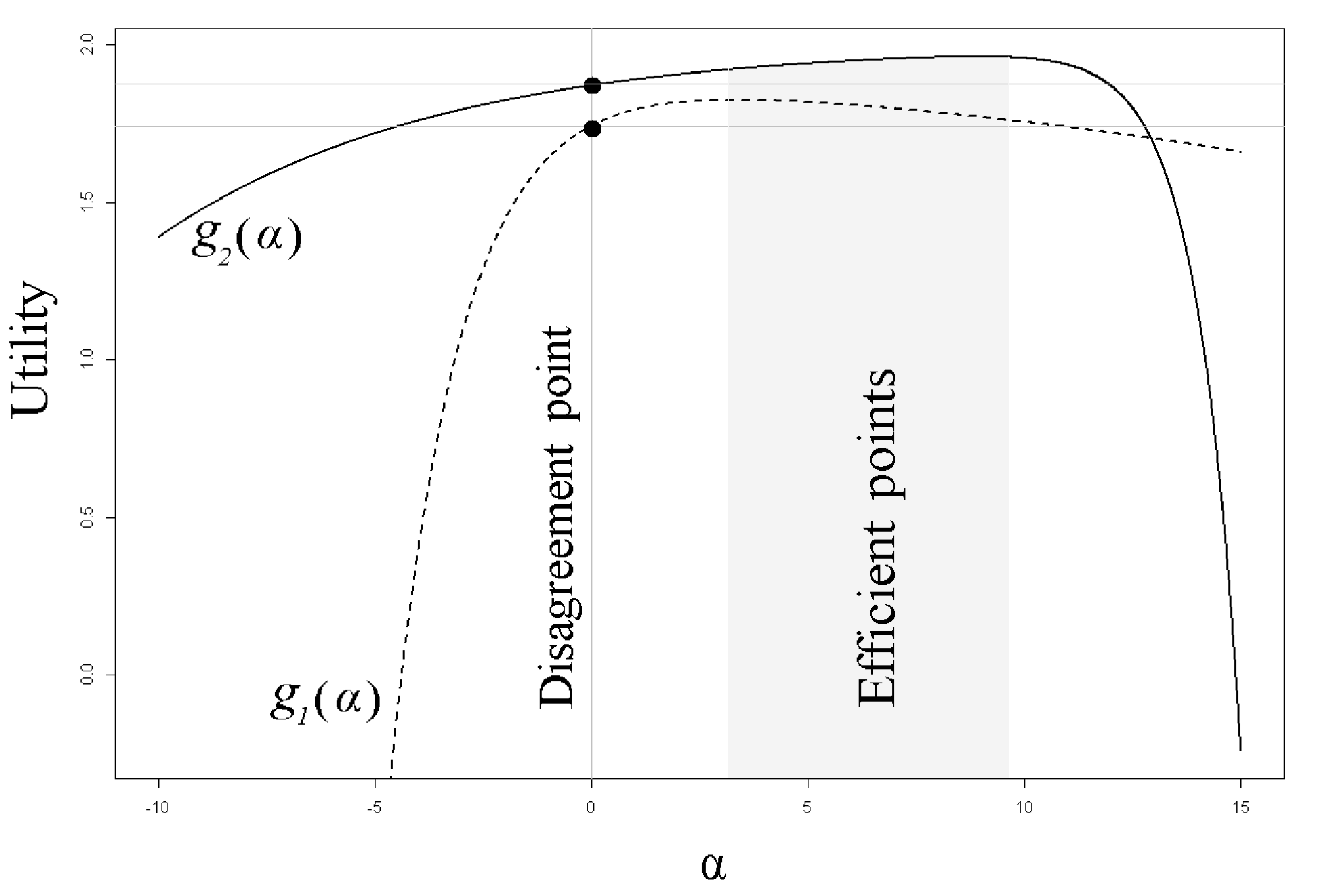
The continuous optimal step lengths for the two respective agents are argmax and argmax . Due to the unimodality of , all efficient solutions of (32) are given by integer step lengths (see Fig. 1), i.e., for we have
Due to the unimodality of both utility functions with respect to , no efficient solution exists for an outside the segment .
The above example illustrates a case where the segment between and contains five integer points, associated with the feasible step lengths.
The following statements give a constructive characterization of the Pareto frontier of an ERP for the case of concave utility function and linear utility functions respectively.
Corollary 1.
Let be the set of integer points in the interval , where , and , , and let be the interval of feasible step lengths defined in (26). Then, due to Proposition 2, the set of Pareto efficient solutions of an ERP can be obtained as follows:
- i.
if is not empty and does not contain the zero.
- ii.
If is empty and there exists an integer point between and but no integer point between and then contains the unique point given by such that is the greatest integer between 0 and .
- iii.
If is empty and there exists an integer point between and but no integer point between and then contains either the unique point given by such that is the smallest integer between and , or , or both of them if they do not dominate each other. (In this case the three possibilities must be checked, since if for only one of the utilities —let it be , for instance— , being the smallest integer between and , then both values and are Pareto efficient.)
- iv.
If is empty and there are integer points both between and and between and then contains the points given by such that is either the smallest integer between and , or the greatest integer between 0 and , or both points if they do not dominate each other.
- v.
In the case that contains the zero, then no point dominates the initial endowment , so that the only point in the Pareto frontier is .
Corollary 2.
Consider the case of an economy where agents have linear utility functions with gradients and let again be the set of integer points in the interval , where , and , , and let be the interval of feasible step lengths defined in (26). It might be easily seen that either or . The set in the case and have opposite sighs, whereas if and have the same sign. Then, due to Proposition 2, the set of Pareto efficient solutions of an ERP may contain at most one point:
- i.
if there is at least one non-null integer between , and , and , then only contains the unique point corresponding to the allocation for a step-length which is either equal to , (if - and - are negative) or for equal to , (if - and - are positive).
- ii.
only contains the disagreement point in the opposite case.
Having a characterization of the Pareto frontier for any ERP in the sequence allows not just a higher efficiency in simulating the process but also the possibility of measuring the number of non dominated endowments of each of the ERPs, which might be used as a measure of uncertainty of the process. Indeed, the uncertainty of a barter process of this type might come from different sides: i) how to choose the couple of agents and commodities in each step? ii) which Pareto efficient solution of each ERP to use to update the endowments of the system? In the next subsection we shall study different criteria for answering the first two questions.
Note that the set of non-dominated solutions of the ERP, obtained by the local search movement (24) might give rise to imbalances between supply and demand, as described by Dreze [12] for the continuous case. To resolve this imbalance Dreze introduce a quantity rationing, which can by also extended to the ERP.
Consider a rationing scheme for the ERP as a pair of vectors , , with , such that the and ER verifies , for , where and are the components of and respectively. Thus, for two given agents and and two given commodities and we have
| (33) |
An open problem which has not been is not investigated by Nasini et al. [21] is the formulation of equilibrium conditions for this rationing scheme. One possibility might be the construction of two intervals for and which minimize the overall imbalances, under the conditions that (33) is verified in each ERP, as long as and are inside the respected intervals. The integrality of the allocation space forbids a straightforward application of the equilibrium criteria proposed by Dreze [12] to the markets we are considering in this work.
2.3 Direction of movement: who exchange what?
The sequence of elementary reallocations formalized in (21) requires the iterative choice of couples of agents and couples of commodities , i.e., directions of movement among the in the neighborhood of the current solution. If we this choice is based on a welfare function (summarizing the utility functions of all the agents), the selection of of couples of agents and couples of commodities can be made mainly in two different ways: first improving and best improving directions of movement.
The best improving direction requires an exhaustive exploration of the neighborhood. Noting that each direction of movement in the current neighborhood constitutes a particular ERP, a welfare criterion might be the uncertainty of each elementary reallocation, measured by the number of points in the Pareto frontier of ERPs, as described in the previous subsection. A usual welfare criterion is a norm of the objective vector (e.g., Euclidean, or norms). Also the average marginal rate of substitution could represent an interesting criterion to select the direction of movement as a high marginal rate of substitution suggests a kind of mismatch between preferences and endowments.
If at iteration an improving direction exists the respective endowments are updated in accordance with the solution of the selected ERP: for each couple of commodities and each couple of agents , agent gives units of to agent and in return he/she gets units of , for some . At iteration , a second couple of commodities and agents is considered in accordance with the defined criterion. If we use a first improving criterion, the process stops when the endowments keep in status quo continuously during explorations, i.e., when no improving direction is found in the current neighborhood.
2.4 Linear utilities
In microeconomic theory the utility functions are rarely linear, however the case of linear objectives appears particularly suitable from an optimization point of view and allows a remarkable reduction of operations, as the ERPs cannot have more than one Pareto-efficient solution (see Corollary 1).
Consider a given direction of movement . We know that a feasible step length belongs to the interval defined by (26). Since in the case of one linear objective the gradient is constant, for any direction of movement the best Pareto improvement (if there exists one) must happen in the endpoints of the feasible range of (let and denote the left and right endpoints of the feasible range of , when the direction of movement is ). Therefore, the line search reduces to decide either , or none of them. Then for every given point , we have a neighborhood of at most candidate solutions.
Despite the idea behind the SER is a process among self-interested agents, which are by definition local optimizers, this algorithm could also be applied to any integer linear programming problem with one linear objective: . In this case however the branch and cut algorithm is much more efficient even for big instances, as we will show in the next section.
If a first-improve method is applied, an order of commodities and agents is required when exploring the neighborhood and the equilibrium allocation might be highly affected by this order (path-dependence). The pseudocode of algorithm 1 describes the first improve search of the barter algorithm applied to the case of one linear objective function.
Note that if the nonnegativity constraints are not taken into account, problem (2) is unbounded for linear utility functions. This corresponds to the fact that without lower bounds the linear version of this problem would make people infinitely get into debt. As a consequence, the only possible stopping criterion, when the objective function is linear, is the fulfillment of nonnegativity constraints, i.e. a given point is a final endowment (an equilibrium of the barter process) if we have that for any direction of movement and for any given integer if then has some negative component. In some sense the optimality condition is now only based on feasibility.
2.5 The final allocation and the convergence of the SER
For the case of a continuous commodity space and exogenous prices, pairwise optimality implies global optimality, as long as all agents are initially endowed with some positive amount of a commodity [14]. Unfortunately, the SER described in this paper does not necessarily lead to Pareto efficient endowments. Let , representing a simultaneous reallocation of commodities among agents, with step length for each couple of commodities and agents , starting from . Whereas a SER is required to keep feasibility along the process, a simultaneous reallocation of commodities among agents does not consider the particular path and any feasibility condition on the paths leading from to . Hence, remembering that all SERs described in this section stop when no improving elementary reallocation exists in the current neighborhood, we can conclude that the non existence of a feasible improving ER does not entail the non existence of an improving simultaneous reallocation of commodities among agents. In this sense a SER provides a lower bound of any sequence of reallocations of more than two commodities and two agents at a time.
Consider the Lyapunov function , associating a real value to each point in the allocation space [29]. As increases monotonically along the SER (24) and the allocation space is a finite set, then .
Some understanding of the evolution of along the SER iteration can be provided.
Proposition 3.
Consider a SER with commodities among agents with linear utility functions, i.e. , where (the utility functions can be rescaled by a common constant without affecting the SER). The change in the Lyapunov function from iteration to iteration is bounded from above by
| (34) |
where and are the minimum and maximum elements of , for , as defined in (2); is the minimum price and .
Proof.
Let be the direction of movement selected at iteration of the SER, the corresponding allocation and be the change in the Lyapunov function from iteration to iteration . In the general case we have
| (35) |
which the case of linear utility functions (i.e. ) becomes
| (36) |
in accordance with (26). Based on Corollary 2, we have
| (37a) | |||
| if - and - are negative. | |||
| (37b) | |||
| if - and - are positive. | |||
Without lose of generality, let (prices can be rescaled by choosing one commodity as a numeraire). Then, in the economically meaningful case of having , for , we have
| (38) |
since , for all and . ∎
In the economically meaningful case of , for all , the immediate economical interpretation of this result is that a high rage of variation of prices might result in big changes of the aggregated utility, from one bilateral exchange to another. The effect of the variability of prices on the computational performance of the SER will be studied in Subsection 4.2.
3 Bartering on networks
An important extension of the problem of bargaining integer amounts of commodities among agents with fixed prices is to define a network structure such that trades among agents are allowed only for some couples of agents who are linked in this network. In this case the conservation of commodities is replaced by balance equations on a network, so that the final allocation of commodity must verify , where is the flow of commodity in the system, is the incidence matrix, and is a diagonal matrix containing the weights of the conservation of commodity , that is (for more details on network flows problems see [1]).
It is also possible for the final allocation to have a given maximum capacity, that is, an upper bound of the amount of commodity that agent may hold: .
The variables of the problem are now , which again represent the amount of commodity hold by agent , which are the slack variables for the upper bounds, and which are the flow of commodity from agent to agent .
The objective functions , might depend on both the final allocation and the interactions , since the network topology could represent a structure of geographical proximity and reachability.
The resulting mathematical programming formulation of the problem of bargaining integer commodities with fixed prices among agents on a network with upper bounds on the final allocations is as follows:
| (39a) | |||
| s. to
| |||
| (39b) | |||
| (39c) | |||
where , , , , , , and . Matrix is an appropriate permutation of the diagonal matrix made of copies of the matrix with the weights of the conservation of commodity and is the utility function of agent evaluated in the initial endowments with null flow.
Problem (2) had variables and constraints, whereas problem (39) has variables and constraints. When a SER is applied, the definition of a network structure and the application of upper bounds to the final allocation reduce the number of feasible directions of movement in each iteration and the bound of the interval of feasible step length, as for any incumbent allocation , the step length must be such that .
The effect of network structures on the performance of a barter process has been previously studied by Bell [6] and by Wilhite [31], for the case of endogenous prices and continuous commodity space. In this case the process takes into account how agents update prices each time they perform a bilateral trade. Reasonably, prices should be updated based either on the current state of the only two interacting agents or on the state of the overall population or also on the history of the system, such as previous prices. Bell showed that centralized network structures, such as a stars, exhibit a faster convergence to an equilibrium allocation.
It must be noted that any sequence of bilateral trades intrinsically gives rise to a network structure generated by the set of couples of agents interacting along the process. Such a structure might be statistically analyzed in term of its topological properties, as it is done in the next section with a battery of problems of different sizes.
4 Applications in computational economics
The aim of this section is to provide an inclusive application in the field of computational economics of the mathematical programming based models and methods proposed thus far. All the data sets used to replicates the results illustrated in this section can be downloaded from
https://www.dropbox.com/sh/qekoyisyz1bzeej/AACHor8HbYU_KbYopTPxTjzca?dl=0,
along with a Java code implementing the previously described SERs. The reader could also modify the codes and independently use the same data to run his modified code and check his hypothesis about social bartering.
4.1 Numerical comparison between the simultaneous reallocation and the SERs
We first consider the number of ERs required to equilibrate the system and study their relationship with the size of the problem. In fact a numerical comparison with a global solver, such as the branch and cut, is provided to evaluate the efficiency of a decentralized barter economy in comparison with the action of a centralized global planner.
We have already seen that a SER can also be applied to any integer linear programming problem of the form (2), where the individual utilities are aggregated in a single welfare function. If this aggregated welfare is defined as a linear function of the endowments of the form , the comparison of the SERs with the standard branch and cut algorithm is easily carried out.
Considering the ERP as the basic operation of a SER and the simplex iteration as the basic operation of the branch and cut algorithm, the comparison between the two methods is numerically shown in Table 1 for three replications of 11 problems with the same number of agents and commodities, which amounts to 33 instances. The branch and cut implementation of the state-of-the-art optimization solver Cplex was used.
| size | initial welfare | first-improve | best-improve | branch and cut | ||||
|---|---|---|---|---|---|---|---|---|
| neighborhood | ERPs | solution | ERPs | solution | simplex | solution | ||
| 10 | 75.134 | 0.66 | 267 | 353.269 | 91 | 365.126 | 87 | 394.630 |
| 10 | 147.958 | 0.84 | 271 | 763.188 | 91 | 767.371 | 12 | 769.861 |
| 10 | 1.205.972 | 0.77 | 375 | 3.925.921 | 74 | 3.844.165 | 70 | 4.060.685 |
| 15 | 297.713 | 0.70 | 1.343 | 1.455.839 | 215 | 1.471.387 | 49 | 1.488.149 |
| 15 | 326.996 | 0.71 | 1.090 | 2.544.271 | 237 | 2.554.755 | 63 | 2.614.435 |
| 15 | 625.800 | 0.71 | 806 | 2.640.317 | 224 | 2.644.008 | 76 | 2.684.016 |
| 20 | 183.573 | 0.67 | 2.759 | 3.432.832 | 378 | 3.425.665 | 110 | 3.525.421 |
| 20 | 1.064.023 | 0.81 | 1.582 | 4.197.757 | 361 | 4.194.187 | 94 | 4.331.940 |
| 20 | 201.377 | 0.78 | 2.629 | 1.017.906 | 351 | 1.089.860 | 80 | 1.180.977 |
| 25 | 228.365 | 0.89 | 4.358 | 2.221.790 | 648 | 2.226.152 | 237 | 2.271.552 |
| 25 | 687.492 | 0.65 | 2.806 | 3.416.982 | 572 | 3.403.937 | 113 | 3.462.043 |
| 25 | 323.495 | 0.61 | 4.706 | 2.262.657 | 666 | 2.245.817 | 50 | 2.474.429 |
| 30 | 973.955 | 0.79 | 6.648 | 5.428.473 | 975 | 5.427.207 | 101 | 5.377.843 |
| 30 | 1.811.905 | 0.82 | 13.126 | 8.945.605 | 1.084 | 8.953.611 | 127 | 9.080.651 |
| 30 | 1.302.404 | 0.85 | 12.089 | 7.583.841 | 957 | 7.573.400 | 132 | 7.605.525 |
| 35 | 653.739 | 0.87 | 13.201 | 3.456.918 | 1.310 | 3.458.570 | 112 | 3.474.126 |
| 35 | 564.905 | 0.80 | 8.772 | 3.579.713 | 1.308 | 3.585.815 | 77 | 3.599.639 |
| 35 | 753.056 | 0.83 | 14.199 | 5.132.226 | 1.290 | 5.107.933 | 67 | 5.333.123 |
| 40 | 482.570 | 0.87 | 16.307 | 2.429.707 | 1.608 | 2.428.731 | 145 | 2.446.953 |
| 40 | 430.174 | 0.68 | 7.885 | 5.281.060 | 1.640 | 5.229.740 | 90 | 5.279.631 |
| 40 | 2.795.862 | 0.79 | 14.240 | 19.175.278 | 1.578 | 14.503.963 | 186 | 19.276.444 |
| 45 | 3.392.010 | 0.98 | 62.398 | 22.681.229 | 2.300 | 22.664.443 | 162 | 22.728.195 |
| 45 | 842.645 | 0.92 | 12.900 | 6.606.875 | 2.137 | 6.642.397 | 204 | 6.755.016 |
| 45 | 1.909.859 | 0.97 | 48.688 | 15.979.841 | 2.173 | 15.865.744 | 180 | 16.071.407 |
| 50 | 839.559 | 0.93 | 20.615 | 4.822.082 | 2.105 | 4.859.830 | 137 | 4.895.655 |
| 50 | 718.282 | 0.97 | 20.744 | 3.586.560 | 2.459 | 3.588.633 | 160 | 3.610.194 |
| 50 | 1.570.652 | 0.99 | 58.165 | 18.872.864 | 2.530 | 19.018.519 | 180 | 19.069.868 |
| 55 | 351.051 | 0.98 | 20.344 | 2.761.203 | 2.935 | 2.748.862 | 1.242 | 2.799.187 |
| 55 | 413.656 | 0.96 | 26.780 | 4.566.394 | 2.922 | 4.569.975 | 336 | 4.585.475 |
| 55 | 551.355 | 0.99 | 32.053 | 5.136.295 | 3.139 | 5.135.647 | 253 | 5.157.444 |
| 60 | 468.575 | 0.99 | 27.208 | 1.941.409 | 3.568 | 1.949.786 | 271 | 1.995.930 |
| 60 | 501.366 | 0.99 | 34.323 | 5.051.429 | 3.521 | 5.051.836 | 313 | 5.067.154 |
| 60 | 575.950 | 0.98 | 43.227 | 4.751.072 | 3.589 | 4.747.097 | 273 | 4.801.179 |
The numerical results in Table 1 shows problems where the number of agents and commodities is the same, as reported in the first column. For each of the different sizes replicates are computed.
The second column of Table 1 shows the initial levels of social welfare, . Columns solution give the maximum utility found for the three respective methods (first-improve local search, best-improve local search, branch and cut algorithms).
The first-improve local search results in a reduced neighborhood explorations along the sequence of movements, as suggested by the values in the column neighborhood, which show the proportion of possible combination of agents and commodities explored before moving to an improving direction (in comparison to the whole candidate solutions).
The fourth and fifth columns of Tab. 1, named ’ERP’, reports the number of movements, i.e. the number of ERPs for which the step-length (as defined in (26)) has been non-null. The first-improve local search gives rise to a higher amount of ERPs, in comparison with the best-improve version. In addition, in most of the cases the best-improve search results in better allocations, as their value appear particularly close to the optimal solution (see the seventh and ninth columns of Tab. 1).
On the other hand, when competing with the simultaneous reallocation of all commodities among the agents, the sequence of best-improve elementary reallocations fails to reach comparatively good results in terms of number of elementary operations performed and goodness of the achieved final allocation.
The scatter plots in figures 2 and 3 show the relationship between the problem size (number of agents and commodities) and the elementary operations required for convergence (the ERPs for the best-improve SER and simplex iteration for the branch and cut), with the least square interpolation of algebraical curves and coefficient of determination.
| ERPs (size) |
|---|

| simplex (size) |
|---|

The scatter plots and least square approximation in Fig. 4 and 5 tries to explain the relationship between the problem size and the number of elementary operations (ERPs for the best-improve SER and the simplex pivots for the branch and cut) by an exponential curve of the form , with the corresponding coefficient of determination. The same kind of plots are shown in Fig. 6 and 7 for the least square interpolation of a polynomial curve of the form .
| ERPs size) |
|---|

| simplex size) |
|---|

| ERPs (size |
|---|

| simplex (size |
|---|

This results quite clearly suggest a quadratic growth of the expected ERPs with respect to the size of the problem, in accordance with the a coefficient of determination of . Instead the number simplex iteration of the branch and cut algorithm seems not to be well fitted by any of the proposed curves.
From the same computational view, other sequences of reallocation have been studied by Bell [6], who analyzed the performance of the process under a variety of network structures restricting the interactions to be performed only among adjacent agents. She studied a population of Cobb Douglas’ agents trading continuous amount of two commodities with local Walrasian prices and focused on the speed of convergence to an equilibrium price and allocation, observing that more centralized networks converge with fewer trades and have less residual price variation than more diverse networks.
Bell relied only on the number of trades as a measure of the speed of convergence, which we regarded as movements in the local search formalizing the process. Instead, ten years ago Wilhite [31] also toke into account the cost imposed by searching and negotiating, which we regarded as the exploration of the neighborhood11 1 Note that in the special case of being interested in an aggregate social welfare, a system of many local optimizers (agents) could be highly inefficient if compared with a global optimizer, who acts for the ’goodness’ of the system, as in the case of branch and cut. Also the increase of elementary operation of the barter algorithm is much higher than the one of the branch and cut, particularly when the direction of movement is selected in a best-improve way, as it is shown in Table 1. The economical interpretation suggests that if the time taken to reach an equilibrium allocation is too long, it is possible that this equilibrium is eventually never achieved in real social systems, where perturbing events (change in preferences, appetence of new types of commodities, etc.) might take place..
4.2 The effect of preferences, prices, endowments
The aim of this section is to study how the initial condition of the economy, that is to say, preferences, prices and endowments, are able to affect the computational performance of the barter processes previously defined and the emerging social structure of economical interaction.
A first question when sequences of elementary reallocations are studied might be related to the analysis of which initial condition of the system is more likely to affect the number of non dominated allocations (improving directions), the number of negotiations (neighborhoods explored) and the emerging structure of interaction among agents.
To study the number of non dominated allocations obtained as a result of sequences of elementary reallocations, a method for the enumeration of all possible non-dominated paths from the known initial endowments is described. To do so, the directions are explored in each step in such a way that a bundle non dominated reallocations are kept. Let be the number of non-dominated reallocation in the first iteration; for each a collection of non-dominated directions are obtained. The bundle of non-dominated solutions are thus updated in each wave by adding and allocation in accordance with this enumerative procedure.
This procedure requires a method to find Pareto-optimal vectors each time ERPs are solved. Corley and Moon [10] proposed an algorithm to find the set of Pareto vectors among r given vectors , where , . Sastry and Mohideen [26] observed that the latter algorithm is incorrect and presented a modified version. In our implementation of the the best-improve barter process, we use the modified Corley and Moon algorithm of [26], shown below.
- Step 1.
-
Set , .
- Step 2.
-
If , go to Step 6. For , if , then go to Step 3; else, if , then go to Step 4. Otherwise, go to Step 5.
- Step 3.
-
Set , ; go to Step 2.
- Step 4.
-
If , put and ; go to Step 3. Otherwise, set , where ; set and go to Step 2.
- Step 5.
-
If , put ; go to Step 3. Otherwise, set and go to Step 2.
- Step 6.
-
For , if , then put and stop; else, if , then put and stop; Otherwise, put and stop.
The nice property of the modified Corley and Moon algorithm is that it doesn’t necessarily compare each of the couples of vectors for each of the components. This is actually what the algorithm do in the worst case, so that the complexity could be written as , which is linear with respect of the dimension of the vectors and quadratic with respect to the number of vectors.
The pseudo-code to generate all sequences of elementary reallocations for linear agents, keeping the Pareto-improvement in each interaction, is shown in Algorithm 2.
The function applies the modified Corley and Moon algorithm to a set of utility vectors and allocation vectors and return the Pareto-efficient utility vectors with the associated allocations.
| allocations | utilities | ||||
| iteration 0 | 18 3 3 | 13 4 55 | 22 2 2 | 1422 559 1220 | |
| iteration 1 | 21 3 0 | 10 4 58 | 22 2 2 | 1608 574 1220 | |
| 18 3 3 | 11 4 57 | 24 2 0 | 1422 569 1324 | ||
| iteration 2 | 24 0 0 | 7 7 58 | 22 2 2 | 1800 571 1220 | |
| 19 5 0 | 10 4 58 | 24 0 2 | 1480 574 1326 | ||
| 21 3 0 | 8 6 58 | 24 0 2 | 1608 572 1326 | ||
| 21 3 0 | 8 4 60 | 24 2 0 | 1608 584 1324 | ||
| 21 3 0 | 10 6 56 | 22 0 4 | 1422 567 1430 | ||
| 21 0 3 | 8 7 57 | 24 2 0 | 1614 566 1324 | ||
| iteration 3 | 21 3 0 | 8 4 60 | 24 2 0 | 1608 584 1324 | |
| 22 2 0 | 7 7 58 | 24 0 2 | 1672 571 1326 | ||
| 24 0 0 | 5 9 58 | 24 0 2 | 1800 569 1326 | ||
| 24 0 0 | 5 7 60 | 24 2 0 | 1800 581 1324 | ||
| 24 0 0 | 7 9 56 | 22 0 4 | 1614 564 1430 | ||
| 19 5 0 | 8 4 60 | 26 0 0 | 1480 584 1430 | ||
| 19 5 0 | 10 2 60 | 24 2 0 | 1480 586 1324 | ||
| 21 1 2 | 8 6 58 | 24 2 0 | 1608 582 1430 | ||
| iteration 4 | 21 3 0 | 8 4 60 | 24 2 0 | 1608 584 1324 | |
| 24 0 0 | 5 7 60 | 24 2 0 | 1800 581 1324 | ||
| 19 5 0 | 8 4 60 | 26 0 0 | 1480 584 1430 | ||
| 19 5 0 | 10 2 60 | 24 2 0 | 1480 586 1324 | ||
| 21 1 2 | 8 6 58 | 24 2 0 | 1608 582 1430 | ||
| 21 3 0 | 8 6 58 | 24 0 2 | 1800 579 1430 | ||
| 22 0 2 | 7 9 56 | 24 0 2 | 1672 581 1430 | ||
| 24 0 0 | 7 7 58 | 22 2 2 | 1736 582 1324 | ||
| 20 2 2 | 7 7 58 | 26 0 0 | 1672 583 1324 | ||
| iteration 5 | 21 3 0 | 8 4 60 | 24 2 0 | 1608 584 1324 | |
| 24 0 0 | 5 7 60 | 24 2 0 | 1800 581 1324 | ||
| 19 5 0 | 8 4 60 | 26 0 0 | 1480 584 1430 | ||
| 19 5 0 | 10 2 60 | 24 2 0 | 1480 586 1324 | ||
| 21 1 2 | 8 6 58 | 24 2 0 | 1608 582 1430 | ||
| 21 3 0 | 8 6 58 | 24 0 2 | 1800 579 1430 | ||
| 22 0 2 | 7 9 56 | 24 0 2 | 1672 581 1430 | ||
| 24 0 0 | 7 7 58 | 22 2 2 | 1736 582 1324 | ||
| 20 2 2 | 7 7 58 | 26 0 0 | 1672 583 1324 | ||
| 21 0 3 | 8 7 57 | 24 2 0 | 1544 583 1430 | ||

Consider a barter process of 3 commodities among 3 agents and let the initial endowments be , and . The coefficients of the linear objective functions are , and . Starting from the initial solution, the sequence of two-agent-two-commodity barter leads to the movements of Figure 8.
The scale of grey denotes the utility level. Starting from the initial endowments, 28 different stories of elementary reallocations might be generated, although many of them lead to the same stable allocation (local optima). We found 11 stable allocations which might be reached by some sequence of elementary allocation keeping the Pareto-optimality in each ERP.
We consider a theoretical case where agents with linear utility functions have to trade commodities. The following three factors are taken into account:
- -
: the variability of prices;
- -
: association between and and between and (initial stability);
- -
: association between and and between and (dissortative matching).
The aforementioned factors are measured at three levels and randomized replicates have been simulated for each combination of factors. A multivariate analysis of variance (MANOVA) is performed, considering the two following response variables
- -
: the number of non dominated allocations;
- -
: the number of neighborhoods explored.
The MANOVA results22 2 The multiple analysis of variance is used to compare multivariate (population) means of several combinations of factors. The third and fourth columns of Table 2 report commonly used test statistics which provide a p-value assuming an distribution under the null hypothesis. in Table 2 illustrates the effects and the significance of , corresponding to the association between the initial endowments and the marginal utilities of opposite agents. The correlation between the amounts of the initial endowments and the coefficients of the objective function of the same agent does not appear by itself to have a significant effect on the response variables.
| df | Pillai | approx | p-value | |
|---|---|---|---|---|
| 2 | 0.098426 | 2.3033 | 0.06028 | |
| 2 | 0.034673 | 0.7851 | 0.53624 | |
| 2 | 0.133653 | 3.1867 | 0.01474 | |
| 4 | 0.037110 | 0.4207 | 0.90758 | |
| 4 | 0.070324 | 0.8109 | 0.59384 | |
| 4 | 0.166118 | 2.0155 | 0.04701 | |
| Residuals | 89 |
The graphical illustration in Figure 9 supports the MANOVA results, by showing the values of the two response variables for each level of the factors. The price variability seems to have a non-linear effect to both response variables (left panel). The association between the initial endowment and the marginal utility of the same agent doesn’t seem to produce a consistent change in the number of neighborhoods explored (red line in the central panel), though it does have a clear average linear effect on the number of non-dominated allocations. Differently, the correlation between the initial endowment of an agent and the coefficients of the utility function of the other exhibits negative associations with the two response variables.

This experimental result should interpreted as exploratory and aiming to provide clues and suggestions for further analysis about the effect of the initial condition of the system on the outcomes and performance of the SERs. In this respect, the significant effects of dissortative matching advise for the analysis of the dissortative behavior of the economical interaction network.
Any SER intrinsically gives rise to two types of network structures generated by the set of couples of agents interacting along the process:
- -
the between–node–interaction network (whose edge set is represented by the number of exchanges, that is to say, the number of times a ERP is solved per each couple of agents),
- -
the between–node–flow network (whose edge set is represented by amount of exchanged commodities for each couple of agents).
Both networks can be seen as dynamically changing along the process. Such structures might be statistically analyzed in term of their topological properties. We consider three kind of assortativity measures reflecting the preference for an agent to interact with others that are similar or different in some ways:
- -
: couples of agents with highly different marginal utilities are more often commercial partners: ;
- -
: agents who are more sociable (trade more often) interact frequently with agents who are not sociable: –;
- -
: the more two agents are different with respect to their marginal utilities, the more they are different with respect to their commercial interactions: .
The Greek letter denotes the Euclidean distance, is the Pearson correlation, is the valued of the connection between agent and and is the total value of connections of agent , corresponding to the row of the AM. The numerical values in Table 3 corresponds to the aforementioned assortativities applied to the interaction network, corresponding to the instances of Table 1.
| Size | Between–node–flow | Between–node–interaction | ||||
|---|---|---|---|---|---|---|
| 10 | 0.40 | 0.48 | 0.63 | 0.70 | 0.67 | 0.74 |
| 10 | 0.46 | 0.66 | 0.61 | 0.85 | 0.63 | 0.74 |
| 10 | 0.60 | 0.48 | 0.75 | 0.71 | 0.70 | 0.75 |
| 15 | 0.47 | 0.31 | 0.62 | 0.74 | 0.48 | 0.56 |
| 15 | 0.33 | 0.36 | 0.58 | 0.58 | 0.44 | 0.67 |
| 15 | 0.24 | 0.48 | 0.53 | 0.56 | 0.74 | 0.66 |
| 20 | 0.28 | 0.41 | 0.61 | 0.39 | 0.62 | 0.54 |
| 20 | 0.23 | 0.18 | 0.46 | 0.54 | 0.48 | 0.55 |
| 20 | 0.12 | 0.06 | 0.37 | 0.48 | 0.45 | 0.42 |
| 25 | 0.14 | 0.18 | 0.39 | 0.55 | 0.66 | 0.53 |
| 25 | 0.36 | 0.32 | 0.60 | 0.65 | 0.56 | 0.66 |
| 25 | 0.14 | 0.17 | 0.51 | 0.48 | 0.70 | 0.49 |
| 30 | 0.09 | 0.08 | 0.40 | 0.42 | 0.55 | 0.53 |
| 30 | 0.24 | 0.20 | 0.67 | 0.56 | 0.62 | 0.68 |
| 30 | 0.26 | 0.33 | 0.60 | 0.61 | 0.63 | 0.65 |
| 35 | 0.11 | 0.29 | 0.40 | 0.44 | 0.59 | 0.43 |
| 35 | 0.14 | 0.28 | 0.50 | 0.46 | 0.55 | 0.48 |
| 35 | 0.14 | 0.26 | 0.49 | 0.46 | 0.58 | 0.53 |
| 40 | 0.25 | 0.22 | 0.53 | 0.44 | 0.64 | 0.58 |
| 40 | 0.28 | 0.23 | 0.58 | 0.68 | 0.52 | 0.64 |
| 40 | 0.26 | 0.18 | 0.69 | 0.64 | 0.64 | 0.60 |
| 45 | 0.23 | 0.30 | 0.55 | 0.62 | 0.60 | 0.54 |
| 45 | 0.29 | 0.24 | 0.61 | 0.57 | 0.59 | 0.58 |
| 45 | 0.21 | 0.21 | 0.63 | 0.58 | 0.57 | 0.61 |
| 50 | 0.08 | 0.28 | 0.36 | 0.35 | 0.55 | 0.32 |
| 50 | 0.16 | 0.32 | 0.41 | 0.45 | 0.62 | 0.42 |
| 50 | 0.24 | 0.17 | 0.60 | 0.51 | 0.50 | 0.65 |
| 55 | 0.14 | 0.53 | 0.17 | 0.39 | 0.52 | 0.48 |
| 55 | 0.17 | 0.33 | 0.38 | 0.29 | 0.53 | 0.44 |
| 55 | 0.19 | 0.37 | 0.38 | 0.47 | 0.56 | 0.43 |
| 60 | 0.35 | 0.45 | 0.60 | 0.54 | 0.57 | 0.62 |
| 60 | 0.20 | 0.30 | 0.43 | 0.34 | 0.50 | 0.52 |
| 60 | 0.16 | 0.38 | 0.29 | 0.39 | 0.51 | 0.48 |
The significative effect of (the association between the initial endowment and the marginal utility of the other agent) in the MANOVA of Table 2 seems coherent with the assortativity reported in Table 3, in the vague sense that the difference in the agents marginal utilities is likely to result in high exchange opportunities for agents and, conversely, in many possible convenient allocations (in the sense of Pareto).
Surprisingly, as far as the network corresponding to the between–node–flow is concerned, the assortativity appear comparatively higher then the others. It might be argued that this is due to the fact that nodes with similar marginal utilities have similar abilities in catching the same exchange opportunities existing in the market. An analogous result is observed for the networks corresponding to the between–node–interaction.
Regarding the dissortativity of the between–node–interaction, the values in Table 3 provide a clear connections with the results of Cook et al. [9], who observed that most central nodes (in the sense of eigenvector centrality) were not the most successful in achieving high bargaining power. It can be argued that this achievement relies on his/her connections with poorly connected nodes33 3 This results contradict most social psychological literature showing that, in experimentally restricted communication networks, the leadership role typically devolves upon the individual in the most central position [19, 7], as noted by Bonacich [5]:
in bargaining situations, it is advantageous to be connected to those who have few options; power comes from being connected to those who are powerless. Being connected to powerful others who have many potential trading partners reduces one’s bargaining power.
Note that the goodness of being connected with powerful or powerless neighbors depends on the type of commodity flowing within the network. If the utility of nodes are related to the amount of obtained information, the non rival nature of information suggests a positive association between the power of a node and the power of its neighbors.
The dissortative behavior of the valued networks generated by the barter process can be probabilistically analyzed using conditionally uniform random network models. For each of the three problems of size in Table 1, the results in Table 4 show the sample mean and standard deviation of the clustering coefficient and assortativity coefficient of a sample of valued networks with fixed density (summation of the AM components).
| Network | Property | sample mean | sample std. | observed value | one tail p-value | corr CC – AC |
|---|---|---|---|---|---|---|
| CC | 0.0583 | 0.0099 | 0.0107 | 0.9951 | 0.1075 | |
| AC | -0.0181 | 0.0054 | -0.0454 | 0.0000 | ||
| CC | 0.0613 | 0.0114 | 0.0101 | 0.9951 | -0.0847 | |
| Flow | AC | -0.0196 | 0.0056 | -0.0491 | 0.0000 | |
| CC | 0.0615 | 0.0096 | 0.0390 | 0.9974 | 0.1387 | |
| AC | -0.0188 | 0.0058 | -0.0316 | 0.0379 | ||
| CC | 0.0901 | 0.0092 | 0.0822 | 0.7832 | -0.1125 | |
| Interaction | AC | -0.0220 | 0.0110 | -0.0454 | 0.0220 | |
| CC | 0.1085 | 0.0050 | 0.1125 | 0.0992 | 0.1344 | |
| AC | -0.0221 | 0.0115 | -0.0491 | 0.0027 | ||
| CC | 0.1125 | 0.0042 | 0.1178 | 0.0576 | -0.0250 | |
| AC | -0.0203 | 0.0128 | -0.0326 | 0.0411 |
Similarly, for the same samples of Table 4, the results in Table 5 show the sample mean and standard deviation of the clustering coefficient and assortativity coefficient of a sample of valued networks with fixed row marginal of the AM generated by the -kernel method.
| Network | Property | sample mean | sample std. | observed value | one tail p-value | corr CC – AC |
|---|---|---|---|---|---|---|
| CC | 0.0170 | 0.0031 | 0.0107 | 0.9833 | 0.0462 | |
| AC | -0.0079 | 0.0053 | -0.0454 | 0.0000 | ||
| CC | 0.0177 | 0.0041 | 0.0101 | 1.0000 | 0.0286 | |
| Flow | AC | -0.0064 | 0.0060 | -0.0491 | 0.0000 | |
| CC | 0.0433 | 0.0072 | 0.0390 | 0.7895 | -0.0462 | |
| AC | -0.0144 | 0.0073 | -0.0316 | 0.0092 | ||
| CC | 0.0515 | 0.0182 | 0.0822 | 0.1179 | 0.0067 | |
| Interaction | AC | -0.0251 | 0.0102 | -0.0454 | 0.0339 | |
| CC | 0.0848 | 0.0168 | 0.1125 | 0.0870 | -0.1542 | |
| AC | -0.0173 | 0.0143 | -0.0491 | 0.0254 | ||
| CC | 0.0633 | 0.0169 | 0.6384 | 0.0332 | 0.0932 | |
| AC | -0.0154 | 0.0101 | -0.4786 | 0.0433 |
The results in tables 4 and 5 are quite confirmatory, as the negative values of the CC and AC between row marginal can not be explained based on the supposed conditional randomness.
In a series of computational experiments Kang [18] showed an interesting relationship between the variation at the individual level of a network and its assortative behavior. He found that when actors are connected with similarly central alters, the overall variation at the individual centralities (network centralization) is low.
The global picture emerging from the observed computational results strongly supports the previously discussed micromacro linkages. This is particularly true when the dissortative pattern and the network centralization are taken into account [19, 7, 9, 18]. Indeed, this strategic model of network formation is capable of internalizing many and varied assumption on agent behavior, allowing to test hypothesis on the arising of open and closed network structures from the economical interaction.
5 Summary and future directions
We studied the use of barter processes for solving problems of bargaining on a discrete set, representing markets with indivisible goods and fixed exogenous prices. We showed that the allocation space is characterized by a block diagonal system of linear constraints, whose structural properties might be exploited in the construction and analysis of barter processes. Using Proposition 2 and the characterization of the space of integer solutions of the ERP, we were able to derive a constructive procedure to obtain its Pareto frontier, as shown by Corollary 1 and Corollary 2.
Further research on this topic should include the characterization of the integer points in the null space of a general reallocation problem with fixed prices to obtain a closed form solution of a general problem of reallocating integer amounts of commodities among agents with fixed prices.
An open problem, which has not been investigated in this paper, is the formulation of equilibrium conditions for this rationing scheme proposed in Section 3, as suggested by Dreze [12] for the case of continuous allocation space.
In Section 4 we proposed a mathematical programming model for the problem of reallocating integer amounts of commodities among agents with fixed prices on a sparse network structure with nodal capacities. Further research on this issue should include a mathematical properties of a SER in dealing with markets with sparsely connected agents, as formulated in (39).
References
- [1] Ahuja, R.K. , Magnanti, T.L., Orlin, J.B., (1991). Network Flows: Theory, Algorithms, and Applications. (1st ed.). Englewood Cliffs, Prentice-Hall.
- [2] Arrow, K. J., Debreu, G., (1983). Existence of an equilibrium for a competitive economy, Econometrica, 22, 265–290.
- [3] Auman R., Dreze, J., (1986). Values of Markets with Satiation or fixed prices, Econometrica, 54, 1271–1318.
- [4] Axtell, R., (2005). The complexity of exchange, In Working Notes: Artificial Societies and Computational Markets. Autonomous Agents 98 Workshop, Minneapolis/St. Paul (May).
- [5] Bonacich, P., (1987), Power and Centrality: A Family of Measures, Journal of Mathematical Sociology, 92, 1170–1182.
- [6] Bell, A.M., (1998). Bilateral trading on network: a simulation study, In Working Notes: Artificial Societies and Computational Markets. Autonomous Agents 98 Workshop, Minneapolis/St. Paul (May), 1998.
- [7] Berkowitz, L, (1956). Personality and Position, Sociometry, 19, 210–22.
- [8] Caplin A., Leahy, J., (2010). A Graph Theoretic Approach to Markets for Indivisible Goods, Mimeo, New York University, NBER Working Paper 16284.
- [9] Cook, K. S., R. M. Emerson, M. R. Gilmore, and T. Yamagishi, (1983). The Distri- bution of Power in Exchange Networks: Theory and Experimental Results, American Journal of Sociology , 89:275-305.
- [10] Corley, H. W., Moon, I. D., (1985). Shortest path in network with vector weights, Journal of Optimization Theory and Applications, 46, 79–86.
- [11] Danilov, V., Koshevoy, G., Murota, K., (2001). Discrete convexity and equilibria in economies with indivisible goods and money, Journal of Mathematical Social Sciences, 41, 3, 251–273.
- [12] Dreze J. (1975), Existence of an exchange equilibrium under price rigidities. International Economic Review, 16, 2, 301–320.
- [13] Edgeworth, F.Y, (1932). Mathematical psychics, an essay on the application of mathematics to the moral sciences, (3th ed.) L.S.E. Series of Reprints of Scarce Tracts in Economics and Political Sciences.
- [14] Feldman, A., (1973). Bilateral trading processes, pairwise optimality, and pareto optimality, Review of Economic Studies, XL(4) 463–473.
- [15] Haimes, Y.Y., Lasdon, L.S., Wismer, D.A., (1971). On a bicriterion formulation of the problems of integrated system identification and system optimization, IEEE Transactions on Systems, Man, and Cybernetics, 1(3), 296–297.
- [16] Jevons, W.S, (1888). The Theory of Political economy, (3rd ed.). London, Macmillan.
- [17] Kaneko, M., (1982). The Central Assignment Game and the Assignment Markets, Journal of Mathematical Economics, 10, 205–232.
- [18] Kang, S.M., (2007). Equicentrality and network centralization: A micromacro linkage, Social Networks, 29, 585-601.
- [19] Leavitt, H. J, (1951). Some Effects of Certain Communication Patterns on Group Performance, Journal of Abnormal and Social Psychology, 46:38-50.
- [20] Nash, J.F, (1951). The bargaining problem, Econometrica 18, 155–162.
- [21] Nasini, S., Castro, J., Fonseca i Casas, P., (2014). A mathematical programming approach for different scenarios of bilateral bartering, Sort: Statistics and Operations Research Transactions, 39, 85–108.
- [22] Ozlen, M., Azizoglu, M., (2009). Multi-objective integer programming: a general approach for generating all non-dominating solutions, European Journal of Operational Research, 199(1), 25–35.
- [23] Ozlen, M., Azizoglu, M., Burton, B. A., (Accepted 2012). Optimising a nonlinear utility function inmulti-objective integer programming, Journal of Global Optimization, to appear.
- [24] Quinzii, M., (1984). Core and Competitive Equilibria with Indivisibilities, International Journal of Game Theory, 13, 41–60.
- [25] Rubinstein, A., (1983). Perfect Equilibrium in a bargaining model, Econometrica 50, 97–109.
- [26] Sastry, V.N. , Mohideen, S.I., (1999). Modified Algorithm to Compute Pareto-Optimal Vectors, Journal of Optimization Theory and Applications, 103, 241–244.
- [27] Scarf, H., (1994). The Allocation of Resources in the Presence of Indivisibilitie, Journal of Economic Perspectives, 8, 111–128.
- [28] Shapley, L., Shubik, M., (1972). The Assignment Game I: The Core, International Journal of Game Theory, 1, 111–130.
- [29] Uzawa, H., (1962). On the stability of edgeworth’s barter process, International Economic Review, 3(2), 218–232.
- [30] Vazirani, V., Nisan, N., Roughgarden, T., Tardos, E., (2007), Algorithmic Game Theory, (1st ed.). Cambridge, Cambridge University Press.
- [31] Wilhite, A., (2001). Bilateral trade andsmall-worl-networks,Computational Economics, 18, 49–44.
- [32] Wooldridge, M., (2002). An Introduction to MultiAgent Systems, (1st ed.). Krst Sussex, John Wiley and Sons Ltd.