Connection between in-plane upper critical field and gap symmetry in layered -wave superconductors revisited
Abstract
Angle-resolved upper critical field provides an efficient tool to probe the gap symmetry of unconventional superconductors. We revisit the behavior of in-plane in -wave superconductors by considering both the orbital effect and Pauli paramagnetic effect. After carrying out systematic analysis, we show that the maxima of could be along either nodal or antinodal directions of a -wave superconducting gap, depending on the specific values of a number of tuning parameters. This behavior is in contrast to the common belief that the maxima of in-plane are along the direction where the superconducting gap takes its maximal value. Therefore, identifying the precise -wave gap symmetry through fitting experiments results of angle-resolved with model calculations at a fixed temperature, as widely used in previous studies, is difficult and practically unreliable. However, our extensive analysis of angle-resolved show that there is a critical temperature : in-plane exhibits its maxima along nodal directions at and along antinodal directions at . The concrete value of may change as other parameters vary, but the existence of shift of at appears to be a general feature. Thus a better method to identify the precise -wave gap symmetry is to measure at a number of different temperatures, and examine whether there is a shift in its angular dependence at certain . We further show that Landau level mixing does not change this general feature. However, in the presence of Fulde-Ferrell-Larkin-Ovchinnikov state, the angular dependence of becomes quite complicated, which makes it more difficult to determine the gap symmetry by measuring . Our results indicate that some previous studies on the gap symmetry of CeCu2Si2 are unreliable and need to be reexamined, and also provide a candidate solution to an experimental discrepancy in the angle-resolved in CeCoIn5.
pacs
74.20.Rp, 74.25.Op, 74.70.TxI Introduction
Identifying the precise gap symmetry is generically regarded as an important step on the road of searching for the microscopic pairing mechanism of unconventional superconductivity [1, 2]. Different from the isotropic, phonon mediated BCS superconductors, unconventional superconductors are believed to be induced by the strong electron correlations and normally possess an anisotropic non--wave superconducting gap. Extensive theoretic studies have found that an anisotropic superconducting gap always leads to an anisotropic, angle dependent in-plane upper critical field [3, 4, 5]. Motivated by these studies, the angle-resolved in-plane has recently been widely used to determine the gap symmetry of a number of unconventional superconductors, including cuprate superconductors [6, 7], heavy fermion superconductors [8, 9, 10], iron based superconductors [11], and other types of superconductors such as Sr2RuO4 [12] and K2Cr3As3 [13].
It is widely accepted that cuprate superconductors have a wave gap [14, 15]. However, the precise gap symmetry of many heavy fermion superconductors is still unclear. Among the dozens of known heavy fermion compounds, CeCu2Si2 and CeCoIn5 have attracted special experimental and theoretical interest [16, 17, 18, 19, 20].
As the first heavy fermion superconductor [21], CeCu2Si2 has been studied for more than three decades, but no consensus has been reached concerning its precise gap symmetry. A number of earlier experiments provides evidence for a -wave gap [22, 23]. Subsequent studies of angle-resolved by Vieyra et al. [10] found that the in-plane exhibits a fourfold oscillation with its maxima being along the direction. By fitting model computations to their measurements, Vieyra et al. [10] proposed that the gap symmetry of CeCu2Si2 should be -wave, which is in sharp contrast to most previous works [22, 23]. Recent specific heat measurements suggested that CeCu2Si2 may have a nodeless multi-band superconducting gap [24], which challenges the widely accepted notion that the gap symmetry of this superconductor is -wave. Observations made in the vortex state by scanning tunneling microscopy and spectroscopy are consistent with a multi-band gap with nodes [25]. First-principle calculations speculated that a promising pairing state might be multi-band -wave with loop shaped nodes [26]. Moreover, by measuring the change of penetration depth and renormalized superfluid density, and then comparing these findings to previous measurements of specific heat, a nodeless band-mixing state was also proposed as a candidate for the gap symmetry of CeCu2Si2 [27].
CeCoIn5, discovered in 2001 by Petrovic et al. [28], is known to have one of the highest critical temperature, roughly K, among the whole heavy fermion family. Many experimental measurements, including thermal conductivity [29], specific heat in rotated magnetic field [30], differential conductance [31], inelastic neutron scattering [32], and scanning tunneling microscopy [33, 34], have discovered considerable evidence for a -wave superconducting gap. Angle-resolved in-plane has also been used to probe the gap symmetry of CeCoIn5. However, there is a longstanding experimental discrepancy in the angular dependence of in-plane : some experiments found that the maxima of are along the [110] direction [35], whereas other experiments observed the maxima of along the [100] direction [36, 37, 9]. This discrepancy is regarded as an open puzzle in this field [9, 38], and prevents us from reaching a final consensus on the precise gap symmetry of CeCoIn5.
An external magnetic field couples to the charge and spin degrees of freedom of electrons via the orbital and Zeeman mechanisms, respectively. The former coupling destroys the long-range phase coherence and leads to the mixed state in type-II superconductors. The latter one, called Pauli paramagnetic effect, is believed to play an important role in heavy fermion compounds such as CeCu2Si2 and CeCoIn5 [17, 21, 9, 39, 40]. The behavior of is determined by the interplay of these two effects.
It is well established that the in-plane exhibits a fourfold oscillation in -wave superconductors [4, 5, 6, 7, 8, 9, 10]. In earlier calculations including only the orbital effect [4, 5], was always found to display its maxima along the antinodal directions where the -wave gap is maximal. Later studies included the Pauli paramagnetic effect [9, 41], but still concluded that the maxima of are along the antinodal directions. There appears to be a priori hypothesis in the literature that a larger superconducting gap necessarily results in a larger , which means that and -wave gap should exhibit their maxima (minima) at exactly the same azimuthal angles . If this hypothesized correspondence is valid, it would be easy to identify the gap symmetry: the gap is -wave when the measured exhibits its maxima along the [100] direction; the gap is -wave when the measured exhibits its maxima along the [110] direction.
We emphasize that the above hypothesized connection between in-plane and -wave gap, though intuitively reasonable, is actually not always correct. If there is only orbital effect, and -wave gap do display the same angular dependence. However, this connection can be destroyed by the Pauli paramagnetic effect.
In this paper, motivated by the recent progress and the existing controversy, we will analyze the influence of the interplay of orbital and Pauli paramagnetic effect on the behavior of in-plane in -wave superconductors. The aim of this paper is to provide a better understanding of the properties of the angle-resolved in-plane in CeCu2Si2 and CeCoIn5. After carrying out systematical calculations, we show that the maxima of angle-dependent are not necessarily along the antinodal directions in the presence of Pauli paramagnetic effect. Interestingly, the angular dependence of is determined by a number of parameters, including temperature , critical temperature , gyromagnetic ratio , fermion velocity , and two parameters that characterize the shape of the corresponding Fermi surface. Any of these six parameters can drive a shift in the fourfold oscillation pattern of . Since approximations are inevitable in theoretical calculations, it is technically quite difficult to identify whether the precise gap symmetry is wave or wave by fitting experimental results with model calculations at a fixed temperature. Among the six tuning parameters, the temperature plays a particular role. If one varies but fixes all the rest parameters, exhibits its maxima along the nodal directions at and antinodal directions at due to a sufficiently strong Pauli paramagnetic effect, where is certain critical temperature. The concrete magnitude of may change as other parameters vary, but the existence of a shift in the four-fold oscillation of at appears to be general feature. This feature provides a better method to determine the precise gap symmetry by measuring the in-plane at a large number of temperatures and see whether there is a shift in its angular dependence.
On the basis of our theoretical results, we find that some previous conclusions about the precise gap symmetry of CeCu2Si2 are actually unreliable, and need to be further studied. Moreover, our finding provides a possible solution for an experimental discrepancy in the measured angular dependence of in-plane in CeCoIn5.
To examine the validity of our conclusion, we will also study the impacts of Landau level mixing and Fulde-Ferrell-Larkin-Ovchinnikov (FFLO) state [42, 43], which may be important in some heavy fermion compounds. We find that Landau level mixing does not change the general feature that the maxima of shifts by at critical temperature . In the presence of FFLO state, however, the maximum of may be along the nodal or antinodal directions, depending sensitively on the temperature of the system. This makes it more difficult to identify the precise gap symmetry by measuring the angular dependence of .
The rest of paper is organized as follows. In Sec. II, we derive the equation of in-plane for superconductor with a rippled cylindrical Fermi surface. In Sec. III, we show the influence of different parameters on by numerical calculations. In Sec. IV, the influences of Landau level mixing and FFLO state on are given. In Sec. V, we then compare our results with experimental studies about angle-resolved . In Sec. VI, we summarize our main results.
II Derivation of the equation of
Many heavy fermion compounds have a layered structure, but the inter-layer coupling cannot be entirely ignored [18, 19, 44]. To embody this feature, it is convenient to assume a rippled cylindrical Fermi surface, which is schematically shown in Fig. 1. Now the fermion momentum should have three components: denote the -components in the basic superconducting plane, and denotes the -component along -axis. We use to represent the inter-layer hoping parameter and the unit size along -direction. The dispersion relation of fermions is given by [46, 45],
| (1) |
with . Superconductivity is entirely suppressed once the in-plane field reaches , which can be obtained by solving a linearized gap equation. Near the second-order transition, the gap function has the form
| (2) |
where reflects the symmetry of the gap function and may correspond to , , , and so on. Employing the general methods presented in Refs. [47, 48, 50, 49, 51, 52, 53, 54], we find the following equation
| (3) | |||||
In the simplest case, we now neglect the influence of Landau level mixing and FFLO state. Their influence will be considered separately in Sec.IV. Assuming that , we have
| (4) |
where is the lowest Landau level, and is the angle between the direction of in-plane magnetic field and the -axis, corresponding to the [100] direction, within the basal plane. The generalized derivative operator is defined as
| (5) |
where the vector potential is chosen to be
| (6) |
Now the field takes the form
| (7) |

For a rippled cylindrical Fermi surface, the vector of Fermi velocity is given by [46]
| (8) |
Here, , and , where with Fermi momentum being related to Fermi energy by . The shape of rippled cylindrical Fermi surface is characterized by a velocity ratio , where and . As will be shown later, both and can strongly affect the behavior of . Moreover, we define , where is Bohr magneton and gyromagnetic ratio. The orbital effect is encoded in the factor , whereas the Pauli paramagnetic effect is represented by the factor . The concrete angular dependence of is determined by the interplay of these two effects.
To facilitate analytical computation, we can choose the direction of field as a new -axis and define
In the coordinate frame spanned by , we write the velocity vector as
and the generalized derivative operator as
| (13) | |||||
where
| (14) | |||||
| (15) |
which satisfy
| (16) |

In Eq. (3), the influence of gap symmetry is reflected in . For -wave gap, ; for -wave gap, ; for -wave gap, . Now we take -wave gap as an example, so . The results for -wave gap can be obtained analogously, and the main conclusion does not change. Averaging over on both sides of Eq. (3) and inserting , we obtain
| (17) | |||||
where , and . For the detailed derivation of Eq. (17), please see the Appendix.
Although the linearized gap equation (17) is formally general and valid in many superconductors, its solution is determined by a number of physical effects and associated parameters. From Eq. (17), we see depends on six physical parameters: critical temperature , temperature ratio , velocity , gyromagnetic ratio , , and . Among these parameters, and are related to the shape of the rippled cylindrical Fermi surface. We notice that the influence of and were not carefully investigated in previous works on . x

In previous studies on this problem [8, 9, 10], a rippled cylindrical Fermi surface is often assumed, but there is not any tuning parameter in the equation of that can characterize how rippled is the Fermi surface. In our equation of , given by Eq. (17), we have introduced two tuning parameters and to characterize the concrete shape of the rippled Fermi surface. In the next section, we will show that whether the maxima of is along the nodal or antinodal direction depends on the specific values of these two parameters. Apparently, the shape of the Fermi surface can significantly influence the angular dependence of , which is not properly considered in previous works. In addition, in previous studies of [8, 9, 10], the precise -wave gap symmetry is identified by comparing theoretical calculations to experimental results of at a fixed temperature. In the next section, we will prove that varying the temperature leads to a shift of angle-resolved . This striking temperature dependence of angle-resolved has not been realized previously. According to this property, measuring and then fitting experiments with model calculations at a given temperature may yield incorrect conclusion about the precise gap symmetry.
III Angular dependence of and its connection with gap symmetry
In this section, we present the numerical results for in-plane by solving Eq. (17) numerically and discuss the influence of various parameters on the angular dependence of .
The detailed behavior of can be clearly seen from its angular dependence. In addition, it is equally important to analyze the difference of between its values obtained at and , i.e., since the maxima and minima of always appear at these two angles. exhibits its maxima at if and at if .
First, we consider only the orbital effect by setting . In this case, the factor appearing in Eq. (17) is equal to unity, . We assume that , , , and , which are suitable parameters for heavy fermion compounds.

After carrying out numerical calculations, we plot the angular dependence of in Fig. 2 at two representative temperatures and . Figure 2 clearly shows that exhibits a fourfold oscillation pattern. The maxima of is always along the antinodal directions for any values of relevant parameters, which means that the angular dependence of orbital effect-induced is exactly the same as that of the gap. This is consistent with previous results of Refs. [4, 5]. Moreover, the positions of peaks are -independent. is a monotonic decreasing function of , since the gap is suppressed as grows. Moreover, is negative for all values of .
We next consider the influence of pure Pauli paramagnetic effect on by setting , which leads to
| (18) |
This equation is completely independent of . The -dependence of is shown in Fig. 3. is not a monotonic function: it first rises with growing , but decreases when is sufficiently large.
Finally we come to the interplay of orbital and Pauli paramagnetic effects, which are both important in some heavy fermion compounds, including CeCu2Si2 and CeCoIn5. As aforementioned, the angular dependence of is determined by a number of tuning parameters. To make the results as transparent as possible, we vary one single parameter at each time and fix all the rest parameters at certain values.
As shown in Fig. 4, under the chosen parameters, the maxima of locates along the antinodal directions at a relatively higher temperature . This behavior is very similar to that in the case of pure orbital effect. However, at a lower temperature , the maxima of is along the nodal directions where the -wave gap vanishes. Two conclusions can be drawn: (i) does not always exhibit its maxima at the angles where the superconducting gap is maximal; (ii) the fourfold oscillation curves of are shifted by as temperature grows across certain critical value .
We see from Fig. 4(c) that first increases with growing , but decreases rapidly once exceeds a critical value. Such a non-monotonic -dependence of is clearly caused by the Pauli paramagnetic effect. Moreover, the difference shown in Fig. 4(d) is positive for small but becomes negative for larger values of .

: It is well known that of heavy fermion compounds is not high, especially when compared with cuprates and iron pnictides. To make a general analysis, we assume varies between 0K and 3K. All the other parameters are fixed. From Fig. 5(a), we find that increases monotonously as grows. As displayed in Fig. 6(a), if is smaller than some critical value, is negative, which means the maxima of are along the antinodal directions. For larger , becomes positive and the maxima of are shifted to nodal directions. Clearly, has important impacts on the angular dependence of .
: We then consider the influence of fermion velocity , which characterizes the strength of the orbital effect. According to Fig. 5(b), is not a monotonic function of , it increases with for small values of but decreases with when is large enough. Therefore, in the presence of of Pauli paramagnetic effect, the increasing of orbital effect does not necessarily suppress . At , the orbital effect is removed, so the Pauli paramagnetic effect entirely determines . is then angle independent, and . For finite , becomes angle dependent and exhibits fourfold oscillation, as a consequence of the interplay between orbital and Pauli paramagnetic effects. As shown in Fig. 6(b), is negative for both small and large values of , but becomes positive for intermediate values of .

: Taking simply leads to the known results obtained in the case of pure orbital effect. From Fig 5(c), we see that monotonously deceases with the increase of , which indicates the Pauli paramagnetic effect always tends to suppress . As depicted in Fig. 6(c), is negative when takes small values but positive when becomes sufficiently large.

: For , the rippled cylindrical Fermi surface reduces to a cylindrical Fermi surface. Figure 5(d) shows that decreases monotonously as increases. It appearers that takes larger values as a three-dimensional superconductor evolves gradually to be quasi-two-dimensional. According to the blue solid line in Fig. 6(d), for given values of other parameters, the maxima of is along the nodal directions for small values of and antinodal directions for large values of .
: As shown in Fig 5(d), is a monotonic function of . Varying can also lead to similar shift in . According to the red dashed line in Fig. 6(d), for given relevant parameters, the maxima of is along nodal directions for small values of and antinodal directions for large values of .


From above results, we know that the detailed angular dependence of in-plane is significantly influenced by a number of physical parameters. The fourfold oscillation pattern of can be shifted by if we tune anyone of these parameters. The fact that may exhibit its maxima along either nodal or antinodal directions denies the naive expectation that always displays the same angular dependence as the -wave gap. Therefore, one should be very careful when fitting theories with experiments, because inaccurate and even wrong conclusions will be drawn if some of the parameters are not properly chosen. Due to the complicated dependence of on various parameters and inevitable approximations employed in the theoretical calculations, it is infeasible to identify the precise gap symmetry solely by measuring the fourfold oscillation of .
The temperature plays a particular role since it is usually the only free parameter in one specific material. Our results show that there is generally a difference in the positions of the maxima of and those of -wave gap for , provided that is sufficiently large. We emphasize that this conclusion does not depend on the specific values of other five parameters. Indeed, those five parameters change the fourfold oscillation of by altering the critical value . However, and -wave gap always exhibit their maxima at exactly the same angles once exceeds , which indicates that the Pauli paramagnetic effect is relatively weak compared to the orbital effect at higher .
In order to better understand this point, we plot the relation between and for several values of velocity in Fig. 7. Since larger represents stronger Pauli paramagnetic effect and larger describes stronger orbital effect, this figure clearly shows how is determined by the competition between the orbital and Pauli paramagnetic effects. The monotonic increase of with growing confirms the conclusion that strong Pauli paramagnetic effect causes the difference between the angular dependence of and -wave gap.
IV The influence of Landau level mixing and FFLO state
In this section, we consider the influence of Landau level mixing and the FFLO state. In contrast to the isotropic -wave superconductors, higher Landau level components of the order parameter are generally mixed in anisotropic superconductors, which was first emphasized by Luk’yanchuk and Mineev [49, 4, 55, 8, 9, 10]. In the case of -wave pairing, symmetry arguments ensure that only the and Landau levels are allowed [55, 8, 9, 10]. FFLO state is a novel superconducting state induced by strong magnetic field where the corresponding Cooper paring has a finite total momentum [42, 43, 54, 56, 57]. In a FFLO state, the superconducting gap is modulated in the real space. There have appeared considerable experimental clues in the past decade suggesting that CeCoIn5 is a possible candidate for the FFLO state [20, 37, 57].
Including the mixing between different Landau levels, the function can be written as [4, 8, 9, 10]
| (19) |
where is the raising operator which is showed in Eq. (14), and is the corresponding admixing parameter of the Landau levels. The corresponding equations for is found to have the form
| (20) | |||||
and
| (21) | |||||
where
| (22) | |||||
| (23) |
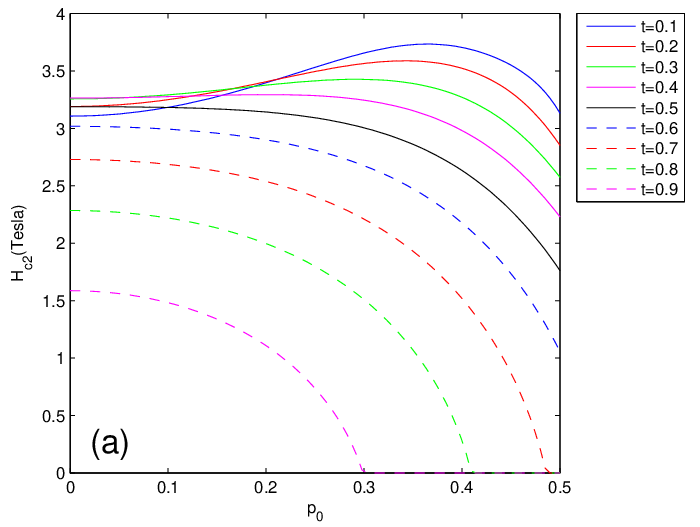
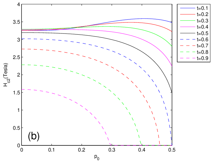
We show the -dependence of , , , and in Fig. 8, where represents the difference of the values of with and without the Landau level mixing effects. The angular dependences of and are plotted in Fig. 9. We find that including Landau level mixing does not change the general feature that the maximum of is along nodal directions at low but along antinodal directions at higher . Figure 8 also shows that is greater than zero, which simply means that the Landau level mixing enhances .
We now consider the impacts of both Landau level mixing and FFLO state. In this case, we should re-write as [9]
| (24) |
The equations for can be obtained by replacing the function appearing in Eqs. (20) and (21) with , where . A detailed derivation of the equations is presented in Appendix A.

The relations between and the FFLO parameter at different temperatures are shown in Fig. 10. Here, is given by , and denotes the physical value of that corresponds to the maximum value of . We find that takes a finite value at lower temperature, however, equals to zero when the temperature is larger than a critical value. After numerical calculation, we find the temperature dependence of , , and , as shown in Fig. 11. It is interesting that, once FFLO state is considered, the angular dependence of can be significantly modified. We can see that the maxima of is along the antinodal directions at low and high temperatures, but along the nodal directions at intermediate temperatures. Apparently, the existence of FFLO state makes it nearly impossible to probe the gap symmetry by measuring at some fixed temperature. Measuring the angular dependence of at a number of different temperatures is thus more reasonable.
V Comparison with experiments
In this section, we compare our results with the experimental studies. There is a longstanding controversy on the in-plane of CeCoIn5. Settai et al. [36] reported that the maxima of are along the [100] direction through de Haas-van Alphen oscillation experiments at mK. Bianchi et al. [37] found the maxima of along the [100] direction by measuring the specific heat at K. Weickert et al. [9] measured the electric resistivity at mK and found the maxima of along the [100] direction. These measurements seem to agree with each other. However, Murphy et al. [35] observed the maxima of along the [110] direction in cantilever magnetometer measurements performed at mK. At first glance, the observation of Murphy et al. [35] is in sharp conflict with other measurements [36, 37, 9], and thus stands as an obstacle in the determination of the precise gap symmetry of CeCoIn5.
Our theoretical analysis suggest that the above experimental results might be actually well consistent. Note that the measurements of Murphy et al.[35] are performed at mK, whereas all the others [36, 37, 9] are performed at mK. The experimental discrepancy can be naturally resolved if, as predicted in our analysis, there is a shift in the angular dependence of at certain temperature between mK and mK. The critical point at which shifts by can be probed by carefully measuring the angular dependence of in-plane at a number of different temperatures falling in the range of .
It is also interesting to remark on the behavior of in CeCu2Si2. Different from a -wave gap symmetry deduced in most earlier investigations [22, 23], a -wave symmetry was proposed by Vieyra et al. [10] after comparing model calculations to the experimental data of measured at mK. This conclusion is problematic for two reasons. Firstly, as illustrated in our theoretic analysis, it is not appropriate to fit experimental results of angle-resolved at some fixed temperature. Secondly, in the equation of given in Ref. [10], a rippled cylindrical Fermi surface is adopted. However, no tuning parameter is adopted in their calculations to characterize how rippled is the Fermi surface. Our analysis indicate that, in order to deduce an accurate gap symmetry from the experiments of in-plane , a more reasonable method is to measure the angular dependence of at a series of temperatures and to see whether there is a shift at certain critical temperature .
VI Summary and Discussion
In summary, we have studied the angular dependence of in-plane upper critical field in some -wave heavy fermion superconductors after including both the orbital and Pauli paramagnetic effects. By solving the equation of systematically, we have showed that whether exhibits its maxima along the nodal or antinodal direction crucially depends on a number of tuning parameters in the presence of a strong Pauli paramagnetic effect. This makes it difficult to entirely fix the -wave gap symmetry, since a moderate variation of one or some of the tuning parameter can lead to a shift in the angular dependence of . Neglecting Landau level mixing and FFLO state, we have found a general property that always exhibits its maxima along the nodal directions at and the antinodal directions at , where is a critical temperature below , provided that the Pauli paramagnetic effect is strong enough. When the Landau level mixing is included, this general property does not qualitatively change. However, the directions of maxima of take more complex dependence on temperature if the superconductor has a FFLO ground state.
Our theoretical studies have gone beyond previous works [8, 9, 10] in several aspects. Firstly, in previous studies, a rippled cylindrical Fermi surface was employed, but there is not any effective parameter in the equations of to characterize the concrete shape of the Fermi surface. In our analysis, the shape of the rippled cylindrical Fermi surface is defined by two parameters, namely and . We have illustrated via careful calculations that tuning these two parameters can qualitatively alter the angular dependence of . Secondly, in previous studies, the angular dependence of was always calculated and then compared with experiments at certain given temperature. Our analysis have showed that whether the maxima of are along nodal or antinodal directions is determined by the values of a number of tuning parameters. Therefore, one should not identify the correct gap symmetry by measuring the angular dependence of at a fixed temperature. Instead, measuring the angular dependence of at a series of temperatures and examining whether there is a shift as the temperature varies is a better method. Thirdly, our studies provide a candidate solution to the long-standing experimental discrepancy about the angular dependence of in CeCoIn5.
To gain a more convincing understanding of the angular dependence of in-plane and its application to realistic experiments of heavy fermion superconductors, our theoretic analysis may be improved in several aspects in the future. For instance, an important assumption used in our analysis is that the superconducting phase transition is second order, which has also been used broadly in previous works [8, 9, 10]. If the phase transition is first order, it would be difficult to derive an effective equation for . In addition, we have employed in our work an ideal rippled cylindrical Fermi surface. It would be very interesting to generalize our consideration to superconductors with a more complicated and more realistic Fermi surface. We have also ignored the possible influence of multi-band effects, which was recently found to be important in several heavy fermion superconductors such as CeCu2Si2 [24, 25, 26, 58] and CeCoIn5 [33, 34]. Finally, our analysis is essentially BCS mean-field treatment, which neglects correlation effects. The possible competition and coexistence between superconducting and antiferromagnetic orders may play some role[53, 59] and hence need to be incorporated in a more refined investigation of .
ACKNOWLEDGEMENTS
We acknowledge the support by the National Natural Science Foundation of China under Grants No.11504379, No.11274286, No.11574285, and No.U1532267.
Appendix A Derivation of equation of in the presence of Landau level mixing and FFLO state
We will provide the detailed calculations of the equation of in-plane in the presence of both Landau level mixing and FFLO state. The linearized gap equation can be written as[52, 54]
| (25) | |||||
where
| (26) |
We assume that takes the FFLO state[9]
| (27) |
with
| (28) |
Here, is along the direction of the magnetic field, namely . Therefore it is easy to get . One can verify that
| (29) |
Substituting Eq. (27) into Eq. (25), we obtain
| (30) | |||||
Exchanging the position of and leads us to
| (31) | |||||
where
| (32) | |||||
| (33) | |||||
| (34) |
In the above derivation, we have used the formula
| (35) |
where and do not commute with each other. If , then commutes with and , namely and . Multiplying on both sides of the Eq. (30), and then moving leftwards and rightwards, we find that
where
| (37) | |||||
It is necessary to make an average of Eqs. (31) and () on the ground state . Since takes the form of the eigenfunction of harmonic oscillators, we can use the formula for harmonic oscillators:
| (38) |
and then obtain
| (39) | |||||
and
Substituting into Eqs. (39) and () and defining , we eventually find that
| (41) | |||||
and
| (42) | |||||
where
| (43) |
References
- [1] M. R. Norman, Science 332, 196 (2011).
- [2] D. J. Scalapino, Rev. Mod. Phys. 84, 1383 (2012).
- [3] L. P. Gorkov, Pis’ma Zh. Eksp. Theor. Fiz. 40, 351 (1984) [Sov. Phys. JETP Letter 40, 1155 (1984)].
- [4] H. Won and K. Maki, Physica B 199-200, 353 (1994).
- [5] K. Takanaka and K. Kuboya, Phys. Rev. Lett. 75, 323 (1995).
- [6] Y. Koike, T. Takabayashi, T. Noji, T. Nishizaki, and N. Kobayashi, Phy. Rev. B 54, R776 (1996).
- [7] T. Naito, S. Haraguchi, H. Iwasaki, T. Sasaki, T. Nishizaki, K. Shibata, and N. Kobayashi, Phys. Rev. B 63, 172506 (2001).
- [8] H. Won, K. Maki, S. Haas, N. Oeschler, F. Weickert, P. Gegenwart, Phys. Rev. B 69, 180504(R) (2004).
- [9] F. Weickert, P. Gegenwart, H. Won, D. Parker, and K. Maki, Phys. Rev. B 74, 134511 (2006).
- [10] H. A. Vieyra, N. Oeschler, S. Seiro, H. S. Jeevan, C. Geibel, D. Parker, and F. Steglich, Phys. Rev. Lett. 106, 207001 (2011).
- [11] J Murphy, M. A. Tanatar, D. Graf, J. S. Brooks, S. L. Bud’ko, P. C. Canfield, V. G. Kogan, and R. Prozorov, Phys. Rev. B 87, 094505 (2013).
- [12] Z. Q. Mao, Y. Maeno, S. NishiZaki, T. Akima, and T. Ishiguro, Phys. Rev. Lett. 84, 991 (2000).
- [13] H. Zuo, J.-K. Bao, Y. Liu, J. Wang, Z. Jin, Z. Xia, L. Li, Z. Xu, Z. Zhu, and G.-H. Cao, arXiv:1511.06169v1.
- [14] C. C. Tsuei and J. R. Kirtley, Rev. Mod. Phys. 72, 969 (2000).
- [15] A. Damascelli, Z. Hussain, and Z.-X. Shen, Rev. Mod. Phys. 75, 473 (2003).
- [16] H. v. Löhneysen, A. Rosch, M. Vojta, and P. Wölfle, Rev. Mod. Phys. 79, 1015 (2007).
- [17] O. Stockert, S. Kirchner, F. Steglich, and Q. Si, J. Phys. Soc. Jpn. 81, 011001 (2012).
- [18] Y. Matsuda, K. Izawa and I. Vekhter, J. Phys.: Condens. Matter 18, R705 (2006).
- [19] J. L. Sarrao and J. D. Thompson, J. Phys. Soc. Jpn. 76, 051013 (2007).
- [20] J. D. Thompson and Z. Fisk, J. Phys. Soc. Jpn. 81, 011002 (2012).
- [21] F. Steglich, J. Aarts, C. D. Bredl, W. Lieke, D. Meschede, W. Franz, and H. Schäfer, Phys. Rev. Lett. 43, 1892 (1979).
- [22] O. Stockert, J. Arndt, A. Schneidewind, H. Schneider, H. S. Jeevan, C. Geibel, F. Steglich, M. Loewenhaupt, Physica B 403, 973 (2008).
- [23] I. Eremin, G. Zwicknagl, P. Thalmeier, and P. Fulde, Phys. Rev. Lett. 101, 187001 (2008).
- [24] S. Kittaka, Y. Aoki, Y. Shimura, T. Sakakibara, S. Seiro, C. Geibel, F. Steglich, H. Ikeda, and K. Machida, Phys. Rev. Lett. 112, 067002 (2014).
- [25] M. Enayat, Z. Sun, A. Maldonado, H. Suderow, S. Seiro, C. Geibel, S. Wirth, F. Steglich, and P. Wahl, Phys. Rev. B 93, 045123 (2016).
- [26] H. Ikeda, M.-T. Suzuki, and R. Arita, Phys. Rev. Lett. 114, 147003 (2015).
- [27] G. M. Pang, M. Smidman, J. L. Zhang, L. Jiao, Z. F. Weng, E. M. Nica, Y. Chen, W. B. Jiang, Y. J. Zhang, H. S. Jeevan, P. Gegenwart, F. Steglich, Q. Si, and H. Q. Yuan, arXiv:1605.04786v1.
- [28] C. Petrovic, P. G. Pagliuso, M. F. Hundley, R. Movshovich, J. L. Sarrao, J. D. Thompson, Z. Fisk, and P. Monthoux, J. Phys.: Condens. Matter 13, L337 (2001).
- [29] K. Izawa, H. Yamaguchi, Y. Matsuda, H. Shishido, R. Settai, and Y. Onuki, Phys. Rev. Lett. 87, 057002 (2001).
- [30] K. An, T. Sakakibara, R. Settai, Y. Onuki, M. Hiragi, M. Ichioka, and K. Machida, Phys. Rev. Lett. 104, 037002 (2010).
- [31] W. K. Park, J. L. Sarrao, J. D. Thompson, and L. H. Greene, Phys. Rev. Lett. 100, 177001 (2008).
- [32] C. Stock, C. Broholm, J. Hudis, H. J. Kang, and C. Petrovic, Phys. Rev. Lett. 100, 087001 (2008).
- [33] M. P. Allan, F. Massee, D. K. Morr, J. Van Dyke, A. W. Rost, A. P. Mackenzie, C. Petrovic, and J. C. Davis, Nat. Phys. 9, 468(2013).
- [34] B. B. Zhou, S. Misra, E. H. da Silva Neto, P. Aynajian, R. E. Baumbach, J. D. Thompson, E. D. Bauer, and A. Yazdani, Nat. Phys. 9, 474 (2013).
- [35] T. P. Murphy, D. Hall, E. C. Palm, S. W. Tozer, C. Petrovic, Z. Fisk, R. G. Goodrich, P. G. Pagliuso, J. L. Sarrao, and J. D. Thompson, Phys, Rev. B 65, 100514(R) (2002).
- [36] R. Settai, H. Shishido, S. Ikeda, Y. Murakawa, M. Nakashima, D. Aoki, Y. Haga, H. Harima, and Y. nuki, J. Phys.: Condens Matter 13, L627 (2001).
- [37] A. Bianchi, R. Movshovich, C. Capan, P. G. Pagliuso, and J. L. Sarrao, Phys. Rev. Lett. 91, 187004 (2003).
- [38] T. Das, A. B. Vorontsov, I. Vekhter, and M. J. Graf, Phys. Rev. B 87, 174514 (2013).
- [39] A. Bianchi, R. Movshovich, N. Oeschler, P. Gegenwart, F. Steglich, J. D. Thompson, P. G. Pagliuso, and J. L. Sarrao, Phys. Rev. Lett. 89, 137002 (2002).
- [40] A. D. Bianchi, M. Kenzelmann, L. DeBeer-Schmitt, J. S. White, E. M. Forgan, J. Mesot, M. Zolliker, J. Kohlbrecher, R. Movshovich, E. D. Bauer, J. L. Sarrao, Z. Fisk, C. Petrović, M. R. Eskildsen, Science 319, 177 (2008).
- [41] A. B. Vorontsov and I. Vekhter, Phys. Rev. B 81, 094527 (2010).
- [42] P. Fulde and R. A. Ferrell, Phys. Rev. Lett. 135, A550 (1964).
- [43] A. I. Larkin and Y. N. Ovchinnikov, Zh. Eksp. Teor. Phys. 47, 1136 (1964) [Sov. Phys. JETP 20, 762 (1965)].
- [44] A. V. Chubukov and L. P. Gor’kov, Phys. Rev. Lett. 101, 147004 (2008).
- [45] A. B. Vorontsov and I. Vekhter, Phys. Rev. B 75, 224501 (2007).
- [46] P. Thalmeier, T. Watanabe, K. Izawa, Y. Matsuda, Phys. Rev. B 72, 024539 (2005).
- [47] E. Helfand and N. R. Werthamer, Phys. Rev. 147, 288 (1966).
- [48] N. R. Werthamer, E. Helfand, P. C. Hohenberg, Phys. Rev. 147, 295 (1966).
- [49] I. A. Luk’yanchuk and V. P. Mineev, Zh. Eksp. Teor. Phys. 93, 2045 (1987) [Sov. Phys. JETP 66, 1168 (1987)].
- [50] K. Scharnberg and R. A. Klemm, Phys. Rev B 22, 5233 (1980).
- [51] H. Shimahara, S. Matsuo, and K. Nagai, Phys. Rev. B 53, 12284 (1996).
- [52] H. Shimahara and D. Rainer, J. Phys. Soc. Jpn. 66, 3591 (1997).
- [53] Y. Suginishi and H. Shimahara, Phys. Rev. B 74, 024518 (2006).
- [54] H. Shimahara, Phys. Rev. B 80, 214512 (2009).
- [55] H. Won and K. Maki, Phys. Rev. B 53, 5927 (1996).
- [56] R. Casalbuoni and G. Nardulli, Rev. Mod. Phys. 76, 263 (2004).
- [57] Y. Matsuda and H. Shimahara, J. Phys. Soc. Jpn. 76, 051005 (2007).
- [58] Y. Tsutsumi, K. Machida, and M. Ichioka, Phys. Rev. B 92, 020502(R) (2015).
- [59] G. Zwicknagl and P. Fulde, Z. Phys. B 43, 23 (1981).