Distance Landmarks Revisited for Road Graphs
Abstract
Computing shortest distances is one of the fundamental problems on graphs, and remains a challenging task today. Distance landmarks have been recently studied for shortest distance queries with an auxiliary data structure, referred to as landmark covers. This paper studies how to apply distance landmarks for fast exact shortest distance query answering on large road graphs. However, the direct application of distance landmarks is impractical due to the high space and time cost. To rectify this problem, we investigate novel techniques that can be seamlessly combined with distance landmarks. We first propose a notion of hybrid landmark covers, a revision of landmark covers. Second, we propose a notion of agents, each of which represents a small subgraph and holds good properties for fast distance query answering. We also show that agents can be computed in linear time. Third, we introduce graph partitions to deal with the remaining subgraph that cannot be captured by agents. Fourth, we develop a unified framework that seamlessly integrates our proposed techniques and existing optimization techniques, for fast shortest distance query answering. Finally, we experimentally verify that our techniques significantly improve the efficiency of shortest distance queries, using real-life road graphs.
I Introduction
We study the node-to-node shortest distance problem on large graphs: given a weighted undirected graph with non-negative edge weights and two nodes of , the source and the target , find the shortest distance from to in . We allow the usage of auxiliary structures generated by preprocessing, but restrict them to have a moderate size (compared with the input graph). In this work, we are only interested in exact shortest distances on large graphs.
Finding shortest distances, a twin problem of finding shortest paths, is one of the fundamental problems on graphs, and has found its usage as a building block in various applications, e.g., measuring the closeness of nodes in social networks and Web graphs [18, 24, 28], and finding the distances between physical locations in road networks [34].
Algorithms for shortest distances have been studied since 1950’s and still remain an active area of research. The classical one is Dijkstra’s algorithm [6] due to Edsger Dijkstra. Dijkstra’s original algorithm runs in [7], and the enhanced implementation with Fibonacci heaps runs in due to Fredman & Tarjan [10], where and denote the numbers of nodes and edges in a graph, respectively. The latter remains asymptotically the fastest known solution on arbitrary undirected graphs with non-negative edge weights [30].
However, computing shortest distances remains a challenging problem, in terms of both time and space cost, for large-scale graphs such as Web graphs, social networks and road networks. The Dijkstra’s algorithm [10] is not acceptable on large graphs (e.g., with tens of millions of nodes and edges) for online applications [24]. Therefore, a lot of optimization techniques have been recently developed to speed up the computation [24, 28, 34, 20, 13, 33, 27, 25, 5].
Distance landmarks (a.k.a. distance oracles, see Section II-B for details) are data structures that support efficient shortest distance query answering, and have been recently studied in both theory [30, 23] and practice [24, 28, 26]. An triangular matrix of size for all-pair shortest distances can be computed in time, using Dijkstra’s algorithm [10], where and are the numbers of nodes and edges, respectively. With the distance matrix, shortest distance queries can be answered in time. This solution, however, is not practical on large graphs: the preprocessing time is too long, and even if one is willing to wait that long, the matrix is too large to be stored effectively. For instance, the matrix of a graph with one million nodes needs about GB memory (here the distance entries are stored as -byte integers).
Distance landmarks aim at striking a balance between the efficiency benefits of answering shortest distance queries and the time and space cost of computing and storing them. And distance landmarks have already been adopted for answering approximate shortest distances [24, 28, 30, 26], and for answering exact shortest distances on directed graphs [14, 23]. However, how to apply distance landmarks for answering exact shortest distances on undirected graphs is mainly limited to pure theoretical analyses [30].
Contributions & Roadmap. To our knowledge, we are among the first to study the application of distance landmarks for fast exact shortest distance queries on large undirected graphs.
(1) We develop an approximation algorithm with a constant factor to analyze distance landmarks by establishing connections with vertex covers (Section III), based on which we show that the direct application of distance landmarks is not practical for large-scale graphs. We then propose hybrid landmark covers, a revised notion of traditional landmark covers, to reduce the space cost (Section III).
(2) We propose a notion of agents such that each agent represents a small subgraph, referred to as deterministic routing areas (dras) (Section IV). Then landmarks are only built for agents, instead of the entire graph. Hence, both space and time cost are reduced. We give an analysis of agents and dras, based on which we develop a linear time algorithm for computing dras along with their maximal agents. As shown in the experimental study, on average about 1/3 nodes of a graph are captured by agents and their dras.
(3) We introduce the bounded graph partitioning problem (bgp) to deal with the remaining subgraph that cannot be captured by the dras of agents, and show that the problem is np-complete (Section V). We then propose a notion of super graphs that combine graph partitions with hybrid landmark covers to support efficient shortest distance answering. We also build connections between the traditional graph partitioning problem and the bgp problem, and utilize the traditional graph partitioning approaches, e.g., Metis, to solve the problem. As shown by the experiments, Metis works well.
(4) We propose a unified framework disLand for fast shortest distance query answering (Section VI), which seamlessly combines distance landmarks with agents, graphs partitions (super graphs), and existing speed-up techniques [34, 32].
(5) Using real-life large road graphs, we conduct an extensive experimental study (Section VII). We find that our disLand scales well with large graphs, e.g., it takes seconds on graphs with nodes and edges. Moreover, disLand is , , and times faster than ch [13], arcFlag [22], and bidirectional Dijkstra [20], respectively. Moreover, the auxiliary structures occupy only a moderate size of space (about of the input graphs), and can be pre-computed efficiently.
Due to the space constraint, we defer all the proofs to [11].
Related work. (1) Algorithms for node-to-node shortest distances have been extensively studied since 1950’s, and fall into different categories in terms of different criteria:
- •
- •
- •
- •
In this work, we study the memory-based exact shortest distance problem on weighted undirected large real-world graphs. None of the previous work has experimentally studied how to apply distance landmarks for solving this problem.
(2) Distance landmarks have been recently investigated for approximate shortest distance queries [30, 24, 28, 26], and for answering exact shortest distances on directed graphs [14, 23]. However, how to apply distance landmarks for answering exact shortest distances on undirected graphs is mainly limited to pure theoretical analyses [30]. Nevertheless, in this work, we investigate how to utilize distance landmarks to speed-up shortest distance queries on real-life large road graphs.
(3) There has recently been extensive work on speed-up techniques for shortest distance queries: bidirectional search [20], hierarchical approaches [13], node and edge labeling [22, 27] and shortcuts [25] (see [34, 32] for two recent surveys). These techniques are complementary to our work, and can be incorporated into our approach. We have indeed seamlessly integrated the ch [13] and arcFlag [22] techniques with distance landmarks into our framework.
(4) Graph partitioning has been extensively studied since 1970’s [17, 16, 35], and has been used in various applications, e.g., circuit placement, parallel computing and scientific simulation [35]. The graph partitioning problem considered in this work differs from the traditional one that it concerns more on the number of nodes with edges across different partitions, instead of the number of edges with endpoints across different partitions. Nevertheless, we build connections between these two problems, and make use of the existing approaches, e.g., Metis [16], to solve the graph partitioning problem considered in this work. It is also worth mentioning that graph partitioning has already been used to speed-up Dijkstra’s algorithm [22].
(5) Agents and deterministic routing areas proposed in this study (Section IV) are significantly different (from definitions to analyses to algorithms) from the 1-dominator sets proposed in [29]. Moreover, the latter are for shortest path queries on nearly acyclic directed graphs, which is not appropriate for real-life large graphs, as these graphs typically contain a large strongly connected components [2].
II Preliminary
In this section, we first present basic notations of graphs. We then introduce the notion of distance landmarks.
II-A Graph Notions
We first introduce graphs and the related concepts.
Graphs. A weighted undirected graph (or simply a graph) is defined as , , , where (1) is a finite set of nodes; (2) is a finite set of edges, in which or denotes an undirected edge between nodes and ; and (3) is a total weight function that maps each edge in to a positive rational number.
We simply denote , , as when it is clear from the context.
Subgraphs. Graph is a subgraph of graph , if (1) for each node , , and, moreover, (2) for each edge , and = . That is, contains a subset of nodes and a subset of edges of .
We also denote subgraph as if is exactly the set of edges appearing in over .
Paths and cycles. A simple path (or simply a path) is a sequence of nodes with no repeated nodes, and, moreover, for each , , is an edge in .
A simple cycle (or simply a cycle) is a sequence of nodes with and no other repeated nodes, and, moreover, for each , , is an edge in .
The length of a path or cycle is the sum of the weights of its constituent edges, i.e., .
We say that (resp. ) is a neighbor of (resp. ).
We also say that a node is reachable to another one if there exists a path between these two nodes.
Shortest paths and distances. A shortest path from one node to another node is a path whose length is minimum among all the paths from to .
The shortest distance between nodes and , denoted by , is the length of a shortest path from to .
Connected components. A connected component (or simply a cc) of a graph is a subgraph in which any two nodes are connected by a path, and is connected to no additional nodes. A graph is connected if it has exactly one connected component, consisting of the entire graph.
Cut-nodes and bi-connected components. A cut-node of a graph is a node whose removal increases the number of connected components in the graph.
A bi-connected component (or simply a bcc) of a graph is a subgraph consisting of a maximal set of edges such that any two edges in the set must lie on a common simple cycle.
II-B Distance Landmarks
We next introduce the notion of distance landmarks [24].
Consider an ordered set of vertices = such that for each , is a distinct node in graph .
We say that is a landmark cover of graph if and only if for any node pair in with reachable to , there exists a landmark () in such that the shortest distance = . This is achieved by representing each node in as a vector of shortest distances to the set of landmarks in . More specifically, each node is represented as an -dimensional vector :
= .
The lmc problem is to find a landmark cover with a minimum number of landmarks in a graph. The problem is unfortunately intractable, as shown below.
Proposition 1: The lmc problem is np-complete [24].
To reduce its computational complexity, an -approximation algorithm was proposed by using the approximation algorithms for the set cover (sc) problem [24]. This algorithm, however, runs in cubic time, and cannot be directly used for large graphs, as already been observed in [24].
Remarks. (1) With a landmark cover , the exact shortest distance for any node pair can be computed in time, where is the number of landmarks in . This is obvious as = + . (2) As a landmark cover occupies space, its size must be small in order to apply it on large graphs.
III Distance Landmarks Revisited
In this section, we first show that it is not practical to directly utilize landmark covers due to the high space cost. We then propose a notion of hybrid landmark covers to alleviate this problem. Here we consider a graph .
III-A Landmark Covers
To give a more accurate estimation of landmark covers, we develop an approximation algorithm with a constant factor . Recall that the sc based algorithm (Section II-B, [24]) has an approximation factor of . To do this, we first present a notion of redundant-edge-free (ref) graphs. We then build the relationship between the lmc problem and the clasical vectex cover (vc) problem on ref graphs, which leads to a -approximation algorithm. Finally, we evaluate the cost of landmark covers with the approximation algorithm.
A vertex cover of a graph is a set of nodes such that each edge of the graph is incident to at least one node of the set. The vc problem is to find a minimum set of vertex covers, a classical optimization problem known to be np-complete [12].
| Graphs | Landmark covers | |||||
|---|---|---|---|---|---|---|
| name | size (mb) | (%) | size (gb) | (s) | ||
| CO | 9.62 | [181,276, 362,552] | [41.6, 83.2] | [588.42, 1,176.83] | [, ] | 34.1 |
| FL | 24.59 | [447,486, 894,972] | [41.8, 83.6] | [3,568.67, 7,137.33] | [, ] | 391.8 |
| CA | 42.54 | [761,662, 1,523,324] | [40.3, 80.6] | [10,730.05, 21,460.09] | [, ] | 1,205.6 |
| E-US | 80.17 | [1,450,115, 2,900,230] | [40.3, 80.6] | [38,880.24, 77,760.48] | [, ] | 4,315.3 |
| W-US | 139.24 | [2,545,995, 5,091,990] | [40.7, 81.3] | [118,786.74, 237,573.47] | [, ] | 12,984.3 |
| C-US | 312.10 | [5,811,428, 1,1622,856] | [41.3, 82.5] | [609,721.69, 1,219,443.38] | [, ] | 66,996.9 |
| US | 531.63 | [9,737,381, 19,474,762] | [40.7, 81.3] | [1,737,359.48, 3,474,718.95] | [, ] | 196,194.6 |
Graphs often contain redundant edges when distance queries are concerned. Graph is redundant-edge-free (ref) if it contains no redundant edges, where an edge is redundant if its removal has no effects on the shortest distance .
By the definition of ref graphs above, it is trivial to see that ref graphs preserve shortest distances, and that a graph may have multiple ref graphs. We next build the relationship between landmark covers and vertex covers, stated as follows.
Theorem 2: For any ref graph , a set of nodes is a landmark cover of iff is a vertex cover of .
As a consequence, the lmc problem is identical to the vc problem on ref graphs.
| Input: | A weighted undirected graph . |
| Output: A landmark cover of . | |
| 1. | Remove redundant edges from ; |
| 2. | Compute a vertex cover of ; |
| 3. | return . |
Approximation algorithm. It is well-known that the vc problem has a 2-approximation algorithm [31], which basically computes a maximal matching of a graph by greedily picking edges and removing all endpoints of the picked edges [6]. Following from Theorem III-A, we obtain a -approximation algorithm for the lmc problem, presented in Fig. 1.
Given a graph , the algorithm first computes an ref graph of by removing redundant edges (line 1). It then computes a vertex cover of the ref graph (line 2), and simply returns as a landmark cover of (line 3).
Note that testing whether an edge is redundant in a graph is typically efficient. When computing using Dijkstra’s algorithm on graph , if for any node before reaching , it is easy to verify that is not a redundant edge. Moreover, for a large portion of edges , its weight is exactly the shortest distance in real-life graphs such as road networks. Hence, our vc based algorithm is typically much faster than the sc based algorithm [24], though they have the same time complexity.
Remarks. The -approximation algorithm allows us to have both lower and upper bounds for the sizes and space cost of landmark covers. If the algorithm returns a landmark cover , then the lower and upper bounds for the size of the optimal landmark cover are and , respectively.
Findings on landmark covers. We next experimentally test the overhead of landmark covers with our approximation algorithm. We tested seven real-life datasets from [8] (please refer to Section VII for details about the datasets and experimental settings). We adopted the adjacency-list representation [6] for graphs when counting their space cost, and assumed that nodes and distances were stored as -byte integers.
The experimental results shown in Table 1 tell us that:
(1) The size of an optimal landmark cover is large, and typically 40%–80% of the nodes in a graph are landmarks.
(2) The space cost of a landmark cover is huge, and is typically more than – times of the graph itself. For instance, the landmark cover of the US graph with GB space may incur a space cost of more than GB.
(3) Computing landmark covers of large graphs is inefficient. It took our algorithm more than 2 days 6 hours on the US dataset. It is worth mentioning that here we only compute the landmarks nodes, not including computing the shortest distances between graph nodes and landmarks. Furthermore, the directly usage of sc based algorithm [24] is even worse, due to its high space and time cost (it even runs out of memory –16GB– for the smallest CO dataset on our testing machine).
Hence, it suffices to conclude that the direct application of distance landmarks as [24] is impractical for large graphs.
III-B Hybrid Landmark Covers
The naive matrix approach stores the pre-computed all-pair shortest distances of a graph , and takes space. And the landmark approach was proposed to reduce the space cost to , where is the size of a landmark cover. One might believe that the landmark approach always incurs less space than the matrix approach. It is, however, not the case as shown by the following example.
Example 1: Consider node in a landmark cover that lies on the shortest paths of a set , , , of node pairs in a graph, where nodes for any . Then node takes space in the naive approach, by directly adding edges to connect those node pairs, while it takes space in the landmark approach, by adding edges between and each of the nodes.
This motivates us to propose a hybrid approach combining the naive approach with the landmark one. To do this, we first define the following notions.
Consider a node in a graph . Let be a set of node pairs such that lies on their shortest paths, and let be the set of distinct nodes in . For a landmark node , we only store the shortest distances between and the node in , instead of all the nodes in the graph as [24]. Hence, the space cost of making a landmark, denoted by , is exactly . Alternatively, the naive approach incurs a space cost of , denoted by , by storing the shortest distances for each node pair in .
Consider an ordered set of vertices = such that (a) for each , is a node in graph , and (b) for any .
Hybrid landmark covers. We say that = is a hybrid landmark cover of graph if and only if:
(1) for each , ,
(2) there exist no other nodes in , but , such that , and
(3) is a set edges, denoting all the node pairs of such that no landmarks in lie on their shortest paths.
We also call = the set of edges enforced by a hybrid landmark cover .
Remark. (1) Essentially, consists of a maximal set of landmarks such that the space cost of each landmark in the set is not larger than the corresponding naive cost.
(2) A hybrid landmark cover of a graph can be treated as another graph with the same set of nodes, but with a different set of edges, i.e., the set of enforced edges. Similarly, the naive approach transforms a graph into a complete graph. This provides a unified view for these two approaches.
(3) Computing hybrid landmark covers on large graphs remains very challenging. Indeed, they cannot be directly used in practice as well. As will be seen in Section V, we build hybrid landmark covers w.r.t. a (small) subset of nodes in graph . In the following, we will explore techniques to support efficient shortest distance queries on large real-life road graphs.
IV Using Representatives for Landmarks
As illustrated and analyzed in Section III, the direct application of distance landmarks is not practical for large graphs. A straightforward approach is to use representatives, each of which captures a set of nodes in a graph. The distance landmarks are for the representatives only, instead of the entire graph, which reduces both space and time cost.
The task to find a proper form of representatives is, however, nontrivial. Intuitively, we expect representatives to have the following properties. (1) A small number of representatives can represent a large number of nodes in a graph; (2) Shortest distances involved within the set of nodes being represented by the same representative can be answered efficiently; And, moreover, (3) the representatives and the set of nodes being represented can be computed efficiently.
In this section, we first propose agents and deterministic routing areas (dras) to capture representatives and the set of nodes being represented, respectively. We then give an analysis of the properties of dras and their agents, and show that they are indeed what we want. Finally, we present a linear-time algorithm for computing agents and their dras. The idea of using agents and dras is illustrated in Fig. 3.
We consider a graph .


IV-A Agents and Deterministic Routing Areas
We first present agents and their dras.
Agents. Given a node in graph , we say that is an agent of a set of nodes, denoted by , if and only if:
(1) node is reachable to any node of in ,
(2) all neighbors of any node are in , and
(3) the size of is equal or less than ,
where is a small constant number, such as or .
Here condition (1) guarantees the connectivity of subgraph , condition (2) implies that not all neighbors of agent are necessarily in ; and condition (3), referred to as size restriction, limits the size of of agent .
Note that a node may be an agent of multiple sets of nodes such that = for any . And we denote as the union of all the sets of nodes whose agent is , i.e., = .
Maximal agents. We say that an agent is maximal if there exist no other agents such that .
Trivial agents. We say that a maximal agent is trivial if contains itself only, i.e., = .
Equivalent agents. We say that two agents and are equivalent, denoted by , if .
Deterministic routing areas (dras). We refer to the subgraph with nodes as a dra of agent .
Intuitively, dra is a maximal connected subgraph connecting to the rest of graph through agent only.
We next illustrate these notions with an example below.
Example 2: First consider graph in Fig. 3, and let = = , where and .
(1) Node is an agent, and its dra is the subgraph in the left hand side of the vertical line across ;
(2) Node is an agent, and its dra is the subgraph in the left hand side of the vertical line across ;
(3) Node is not an agent since it can not find a dra with size less or equal than ;
(4) Node is a maximal agent, while node is not a maximal agent since .
We then consider graph in Fig. 3, and let = = , where and .
(1) Nodes and are three maximal agents, whose dras are all the entire graph , and, hence,
(2) and are three equivalent agents.
Remarks. (1) As illustrated by the above examples, a dra of graph may have a size larger than , and multiple equivalent agents. (2) Trivial agents can only represent themselves. Hence, we are only interested in non-trivial agents (or simply called agents) in the sequel.
IV-B Properties of Agents and DRAs
We next give an analysis of agents and dras, and show that they hold good properties for shortest distance queries.
Proposition 3: Any agent in a graph has a unique dra.
This shows that agents and dras are well defined notions.
Proposition 4: Without the size restriction, any node in graph is a maximal agent, and its dra is exactly the connected component (cc) to which belongs.
This justifies the necessity of the size restriction for agents. Otherwise, dras are simply ccs, and are mostly useless.
Proposition 5:
For any two nodes in the dra of agent in graph ,
(1) the shortest distance in dra is exactly the one in the entire graph ; and
(2) it can be computed in linear time in the size of .
The size restriction guarantees that the shortest distance computation within a dra can be evaluated efficiently.
Proposition 6: Given a node in the dra of agent in graph , and another node in , but not in , the shortest distance = .
Propositions IV-B and IV-B together guarantee that the shortest distances between the nodes in the dras of two distinct agents can be answered correctly and efficiently.
Proposition 7: Any agent in a cc of graph , with must be a cut-node of graph .
This motivates us to identify maximal agents by utilizing the cut-nodes and bccs, which will be seen immediately.
Proposition 8: Any node in a bi-connected component (bcc) with size larger than of graph , is a trivial agent.
As we are interested in non-trivial agents only, those large bccs could be simply ignored with any side effects.
Theorem 9:
Given any two agents and ,
(1) if , then ;
(2) if , then ; and
(3) = , otherwise.
Corollary 10: Given any two maximal agents and , then either or = holds.
This says when maximal agents are concerned, there exists a unique set of non-overlapping dras.
IV-C Computing DRAs and Maximal Agents
In this section, we first present a notion of bc-Sketch graphs, based on which we then propose an algorithm for computing dras and their maximal agents.
The main result here is stated as follows.
Theorem 11: Finding all dras, each associated with one maximal agent, in a graph can be done in linear time.
We shall prove this by providing a linear time algorithm that computes dras and maximal agents. We first present bc-Sketch graphs, a key notion employed by the algorithm.
A bc-Sketch graph of a graph is a bipartite graph, in which (1) = such that is the set of cut-nodes in , and is the set of bccs in ; (2) for each cut-node and each bcc , there exists an edge iff is a cut-node of bcc ; and (3) is a weight function such that for each node , is the number of nodes of in bcc .


Example 3: Consider graph in Fig. 4(1), in which labeled nodes are the cut-nodes of , and the corresponding bccs of are , and , and are shown in Fig. 4(2).
The bc-Sketch graph of graph is shown in Fig. 5, in which = 4, = = = = 2, and = 5.
One may notice that there are no cycles in the bc-Sketch graph . This is not a coincidence, as shown below.
Proposition 12: bc-Sketch graphs have no cycles, which implies that they are simply trees.
Proposition IV-C indicates that we can employ the good properties of trees for computing dras and maximal agents.
| Input: | Graph and constant . | |
| Output: The dras associated with their maximal agents. | ||
| 1. | Find all cut-nodes and bcc nodes of ; | |
| 2. | Build the bc-Sketch graph with = ; | |
| 3. | Identify and return the dras and their maximal agents of . |
| Procedure | |||
| Input: | bc-Sketch graph of graph and constant . | ||
| Output: The dras and their maximal agents of . | |||
| 1. | let be the set of cut-nodes with leaf neighbors in ; | ||
| /* note that a leaf node must be a bcc node */ | |||
| 2. | while is not empty do | ||
| 3. | pick a cut-node from ; let be the neighbors of ; | ||
| /* note that there is at most one non-leaf node in */ | |||
| 4. | let := - + 1; | ||
| 5. | if then | ||
| 6. | merge all bcc nodes in and into one bcc node ; | ||
| 7. | let := ; | ||
| 8. | if there is a non-leaf node in then replace it with ; | ||
| 9. | := ; | ||
| 10. | let be the set of new cut-nodes with leaf neighbors; | ||
| 11. | for each cut-node in do | ||
| 12. | let be a set of leaf neighbors of such that | ||
| 13. | for each , ; | ||
| 14. | mark as the dra of agent ; | ||
| 15. | return all dras with their maximal agents. |
We are now ready to present algorithm shown in Fig. 6. It takes as input graph and constant , and outputs the dras of , each associated with a maximal agent.
(1) Finding cut-nodes and bccs . The algorithm starts with computing all cut-nodes and bi-connected components (line 1), by using the linear-time algorithm developed by John Hopcroft and Robert Tarjan [6, 15].
(2) Constructing bc-Sketch graphs. After all the cut-nodes and bccs are identified, the bc-Sketch graph can be easily built (line 2). To see this can be done in linear time, the key observation is that the number of edges in is exactly since is a tree.
(3) Identifying dras and their maximal agents. Finally, the algorithm identifies and returns the dras and their maximal agents (line 3), using Procedure in Fig. 6.
Procedure takes as input the bc-Sketch graph of graph and constant , and outputs the dras and their maximal agents, by repeatedly merging bccs with size less than . More specifically, the procedure starts with the set of cut-nodes with leaf neighbors (line 1). It then recursively merges the neighboring bcc nodes of cut-nodes to generate new bcc nodes (lines 2-9). For a node with neighbors , if - + , they can be merged into a new bcc node (lines 3-8). Intuitively, this says cut-node is not a maximal agent, and it is combined into the dras of maximal agents. A key observation here is that there is at most one non-leaf node in . If there is such a non-leaf neighbor, then it is replaced by the new bcc node (line 8), by which the merging processing is made possible. Once a cut-node is considered, it is never considered again (line 9). After no merging can be made, we have found all maximal agents, i.e., all the cut-nodes in the updated bc-Sketch graph. We then identify dras for these maximal agents (lines 10-14). For any leaf neighbor of a cut-node , if , then is an of agent . All these together constitute the of agent (lines 12-14). Finally, all dras with their maximal agents are returned (line 15).
We now explain the algorithm with an example as follows.
Example 4: Consider graph in Fig. 4(1) again. Here we let , and = . Firstly, cut-nodes and bccs are computed as shown in Fig. 4(2). Secondly, the bc-Sketch graph of is constructed as shown in Fig. 5. After the merging step stops, the updated bc-Sketch graph consists of three bcc nodes: = , , = and two cut-nodes: and . Finally, the dras and their maximal agents are identified: agent with dra and agent with dra .
Correctness & Complexity. The correctness of algorithm can be readily verified based on the analyses in Section IV-B. To show that algorithm runs in linear time, it suffices to show that procedure can be done in linear time. It is easy to see that each node in the bc-Sketch graph is visited at most twice in procedure , and hence the procedure runs in linear time.
This completes the proof of Theorem IV-C.
Summary. (1) We have proposed a notion of agents and dras aiming at reducing the size of graphs such that landmarks are only for agents, instead of the entire graph. (2) We have given a theoretical analysis of agents and dras, based on which we have developed a linear time algorithm for computing dras and their maximal agents. (3) As shown in our experimental study, on average about 1/3 nodes of a graph are captured by non-trivial agents and their dras.
V Introducing Graph Partitions for Landmarks
Web graphs contain a large strongly connected components [2], and, similarly, there is usually a large bcc in real-life graphs such as the collaboration and social networks [19, 9]. As pointed out in Section IV, for the bccs in a graph with a size larger than , each node in those bccs is a trivial agent that can only represent itself. This motivates us to introduce the graph partitioning techniques for distance landmarks, based on which we use a small set of nodes, instead of a single agent node, to represent a large set of nodes.
In this section, we first introduce graph partitions. We then propose a notion of super graphs which combine graph partitions with hybrid landmark covers. We finally present the bounded graph partition problem and its solution.
We consider a graph .
V-A Graph Partitions and Super Graphs
We first introduce graph partitions and super graphs.
Graph partitions. We say that is a partition of graph if and only if (1) = , and (2) for any , , in which we refer to a () as a fragment of the partition.
We also say that node in () is a boundary node if there exists an edge in from nodes to such that and ().
super graphs. We next introduce super graphs that combine graph partitions with hybrid landmark covers.
Consider a partition of graph . For each fragment (), let (1) be the set of boundary nodes of , and (2) be a hybrid landmark cover for the set of boundary nodes of .
The super graph of graph partition is a weighted undirected graph such that:
(1) = , i.e., the union of all boundary nodes and distance landmarks on each fragment;
(2) = , where is the set of edges with both endpoints belonging to , and for each , is the set of edges enforced by the hybrid landmark cover ; and
(3) For each edge , is exactly equal to the edge weight in graph , and for each edge (), is the local shortest distance between and in the fragment only.
That is, a super graph of graph only consists of the landmarks and boundary nodes. Hence, the size of is typically much smaller than graph . Intuitively, super graphs use a small set of nodes in a fragment, i.e., the boundary nodes and distance landmarks, to represent a large number of nodes, i.e., all the nodes in the fragment.
V-B Bounded Graph Decompositions
As the landmarks are for the boundary nodes, the number of boundary nodes has a key impact on the size of super graphs. In addition, the size of a fragment should be bounded in order to efficiently compute its hybrid landmark cover.
This motivates us to study the following problem.
The bounded graph partitioning problem is to find a partition of graph , denoted by bgp, such that (1) for each fragment (), and (2) , where is a positive integer, is a rational number, and is the total number of boundary nodes.
The problem is, however, nontrivial, as expected.
Proposition 13: The bgp problem is np-complete.
Traditional graph partitioning is to find a partition , , of a graph such that (1) the fragments have a roughly equal number of nodes, and (2) the number of edges connecting nodes in different fragments is minimized. The problem has been extensively studied since 1970’s [17, 16, 35], and has been used in various applications, e.g., circuit placement, parallel computing and scientific simulation [35].
Large-scale graph partitioning tools are available such as the best-known Metis [16]. Hence, this study is not to propose a new graph partitioning algorithm. Instead, it builds relationships between the bgp problem and the traditional graph partitioning problem, and makes use of existing approaches for solving the bgp problem.
Key observations. For any partition , , , the set of boundary nodes with edges across different fragments and the set of all edges connecting nodes in different fragments satisfy: .
This is, minimizing essentially reduces the upper bound of . Moreover, those edges in are part of the super graph. Hence, minimizing also reduces the size of the super graph. This observation inspires us to adopt existing approaches, e.g., Metis [16], to partition graphs and generate super graphs. As will be seen in in our experiments, smaller super graphs help answer shortest distance queries.
Summary. (1) We have introduced a notion of super graphs that combine graph partitions with distance landmarks. (2) We have proposed the bgp problem, and shown it is np-complete. (3) We have also built connections between the bgp problem and the traditional graph partitioning problem, which makes it possible to use the existing approaches, e.g., Metis [16], to solve our problem. As will be seen in our experiments, Metis works well for the bgp problem, and the produced super graphs are typical small, which only have 2–4% nodes and 10–15% edges compared with the original graphs.
VI A Unified Framework for Answering Shortest Distance Queries
In this section, we propose a unified framework, referred to as disLand, for fast shortest distance query answering, which consists of two modules: preprocessing and query answering. We combine distance landmarks with agents and graph partitions (super graphs), and seamlessly integrate existing speed-up techniques [13, 22] into the framework.
Consider a graph with non-negative edge weights.
VI-A Preprocessing for Query Answering
We first present the preprocessing module.
Given graph , the module seamlessly combines agents and graph partitions with hybrid landmark covers, and it produces (a) maximal agents along with their dras, (b) graph partitions, and (c) a super graph .
More specifically, given graph , the module executes the following processes:
(1) It first computes the dras and their maximal agents, using algorithm proposed in Section IV-C.
(2) For each dra with a non-trivial maximal agent , it further (a) computes all the shortest distances for all nodes in its dra, and (b) adds an edge with weight for each node in the dra.
(3) It then generates a shrink graph, the subgraph of in which is the set of agent nodes, including both trivial and non-trivial agents. For each dra with a maximal agent , only is kept in .
(4) It next calls Metis [16] to produce a graph partition for the shrink graph such that for each , is roughly equal to . Here is a small constant number, such as or .
(5) For each fragment (), it computes a (local) hybrid landmark cover for the boundary nodes of only, by calling the sc based algorithm (Section II-B, [24]). Note that here we did not use the vc based algorithm, which was proposed for estimating of the size of landmark covers only.
(6) Finally, it builds a super graph of graph .

The entire process is illustrated in Fig. 7.
VI-B A Bi-level Query Answering Approach
We next present the query answering module.
Given a source node and a target node , this module finds the shortest distance from to , by making use of the auxiliary structures produced by the preprocessing module.
More specifically, given nodes and , the query answering module executes the following processes:
(1) When nodes and belong to the same dra with agent such that = .
If and further fall into the same , then it invokes Dijkstra’s algorithm on the subgraph . Otherwise, it simply returns + in constant time.
(2) When and belong to two dras and with agents and , respectively. As = + + , in which and are already known, we only need to compute .
Let and be the fragments to which agents and belong, respectively. As observed in [4], fragments and and the super graph together suffice to answer exact shortest distance queries. Hence, the algorithm invokes the Dijkstra’s algorithm on the union of subgraphs , and the super graph to compute .
Following the analysis above, we have the following.
Proposition 14: Framework disLand correctly answers shortest distance queries.
VI-C Optimization Techniques
There exist quite a few speed-up techniques for shortest distance computations [32, 34]. disLand is very flexible such that most of these techniques, if not all, can be seamlessly incorporated to further speed-up shortest distance query answering. In this study we have adopted bidirectional search [20], contraction hierarchies (ch) [13], and Arc-Flags (arcFlag) [22] due to their effectiveness and generality.
We first introduce the three optimization techniques.
(1) Bidirectional search (BSearch, [20]) simultaneously performs two searches: forward and backward, starting at the source and target nodes, respectively [20, 32]. It invokes two instances of the Dijkstra’s algorithm simultaneously, and has the same time complexity as the (single directional) Dijkstra’s algorithm. However, BSearch is usually more efficient than the Dijkstra’s algorithm in practice.
(2) Contraction hierarchies (ch, [13]) first imposes a total order on the nodes of a graph, in ascending order of their relative ‘importance’, and then constructs a hierarchy by contracting all the nodes in this order. A node is contracted by removing it from the graph such that shortest paths in the remaining graph are preserved, achieved by replacing paths of the form by a shortcut edge . Note that the shortcut is only required if is the only shortest path from to . After all the nodes are contracted, all the shortcuts are appended into the graph.
ch uses BSearch with minor revisions for query answering. Give two nodes and with , ch only visits two kinds of paths in the process: (a) or (b) there is a unique with and ¿ . In this way, ch avoids visiting the nodes with an order lower than and in the forward and backward searches, respectively, which makes it much more efficient than BSearch alone in practice.
(3) Arc-Flags (arcFlag, [22]) is a partition-based edge labeling approach, and it divides a graph into partitions and gathers information for each edge and for each fragment () on whether the edge lies on a shortest path into the fragment . To do this, each edge is associated with a flag vector with bits (the number of fragments) such that the vector contains a flag 1 or 0 for indicating whether or not is useful for a shortest path query to nodes in . It is easy to verify that arcFlag incurs bits of extra space.
We next show how to seamlessly incorporate these three optimization techniques into our framework disLand.
(1) The shrink graph of graph is appended with shortcuts, by using the ch approach.
(2) We build a hybrid landmark cover for each fragment, by incorporating the ch searching process.
We only consider the shortest paths = such that (a) , in which case is called order rising, or (b) ¡ and ¿ , in which case is called order turning. When computing landmarks for a fragment, we cover a node pair only if (1) there exists an order rising or turning path between and , and (2) their (local) shortest distance in the fragment is equal to their (global) shortest distance in the entire shrink graph. Moreover, (a) for these node pairs connected by order turning paths, we select the nodes with highest order as landmarks; and (b) for these remaining node pairs connected by order rising paths, we use the cost model to greedily select landmarks or build direct edges, following the hybrid landmark approach. As the searching space is reduced, this both improves the efficiency of computing hybrid landmark covers, and, of course, the query answering. Moreover, we adopt the query answering approach for ch [13], instead of the bidirectional Dijkstra’s algorithm, in the query answering module of disLand.
(3) We compute edge labeling, by using the arcFlag approach. To do this, we further call Metis to do a second level partition of the super graph, where each fragment is treated as a single node, and the edge weight between fragments are the number of edges connecting them. When building Arc-Flags, we again incorporate ch, by considering order rising or turning shortest paths only, to speed-up the processing.
Extra space analysis. This module produces two kinds of auxiliary structures: the non-trivial maximal agents along with their dras and the super graph .
(1) Let be the set of non-trivial maximal agents identified. The extra space of and their dras is the extra edges from those agents to the set of nodes in their dras, which is exactly equal to - .
(2) Each fragment in the partition roughly has the same size of . We set = or in practice. Hence, the number of fragments is less than .
For each fragment (), let be the set of edges enforced by the hybrid landmark cover for the boundary nodes of . Hence, the number of extra edges in the super graph is bounded by .
(3) The remaining extra space is incurred by the shortcuts added by ch and the Arc-Flags added by arcFlag.
As will be shown in our experiments, all these auxiliary structures only incur a small space cost, and the entire preprocessing can be finished in a reasonably fast way.
VII Experimental Study
We next present an extensive experimental study of the disLand framework for shortest distance query answering. Using real-life road networks, we conducted five sets of experiments to evaluate: (1) the impacts of agents, graph partitions, and hybrid landmark covers; (2) the preprocessing time and space overhead of bidirectional Dijkstra [20], ch [13], arcFlag [22], their counterparts using agents (Agent + Dijkstra, Agent + ch, Agent + arcFlag), and disLand; and (3) the performance of all these approaches.
VII-A Experimental Settings
We first introduce the settings of our experimental study.
| Name | Regions | # of Nodes | # of Edges |
|---|---|---|---|
| CO | Colorado | 435,666 | 1,042,400 |
| FL | Florida | 1,070,376 | 2,687,902 |
| CA | California & Nevada | 1,890,815 | 4,630,444 |
| E-US | Eastern US | 3,598,623 | 8,708,058 |
| W-US | Western US | 6,262,104 | 1,5119,284 |
| C-US | Central US | 14,081,816 | 33,866,826 |
| US | Entire US | 23,947,347 | 57,708,624 |
Real-life graphs. We chose seven datasets of various sizes from the Ninth DIMACS Implementation Challenge [8], shown in Table 2. Each dataset is an undirected graph that represents a part of the road network in the United States (US), where each edge weight is the distance (integers) required to travel between the two endpoints of the edge.
Distance queries. We adopted the query generator in [34]. Our distance queries were generated as following. On each road network, we generated eight sets , , , of queries. (1) We first imposed a grid on the road network and computed the side length of each grid cell. (2) We then randomly chose ten thousand node pairs from the road network to compose , such that the grid distance of all node pairs in is in . Note that the grid distance of two nodes in a query set is the distance of the cells into which and fall, respectively. Moreover, the grid distance of any node pair in is larger than the grid distance of all node pairs in . For each query set , we report the average running time of over all the ten thousand queries in the set.
Algorithms. We adopted the latest version of Metis [21], implemented with ANSI C. We also re-implemented the original ch [3] from its inventors of using Microsoft Visual C++. Bidirectional Dijkstra, arcFlag and their counterparts using agents were also written in Microsoft Visual C++. All these algorithms used common data structures and procedures, borrowed from ch [3], for similar tasks.
All experiments were run on a PC with an Intel Core i5-2400 CPU@3.10GHz and 16GB of memory. Each test was repeated over 5 times, and the average is reported here. We compare algorithms running on general commercial PCs with a 16GB memory limitation, and hence, algorithms using larger memory, e.g., [1], are not in our consideration.
VII-B Experimental Results
We next present our findings. In all experiments, we tested the datasets in Table 2, and fixed the constant when computing agents and graph partitions on graphs .
| Graphs | Agents (#, %) | Nodes (#, %) in dras | (s) |
|---|---|---|---|
| CO | (56,277, 12.9%) | (156,329, 35.9%) | 1.1 |
| FL | (140,379, 13.1%) | (378,937, 35.4%) | 3.7 |
| CA | (273,191, 14.4%) | (623,811, 33.0%) | 11.3 |
| E-US | (546,481, 15.2%) | (1,228,876, 34.1%) | 34.3 |
| W-US | (869,904, 13.9%) | (2,116,339, 33.8%) | 100.4 |
| C-US | (2,034,358, 14.4%) | (4,583,413, 32.5%) | 402.4 |
| US | (3,452,222, 14.4%) | (7,927,453, 33.1%) | 1153.7 |
Exp-1: Impacts of agents. In the first set of experiments, we evaluated (1) the number of non-trivial agents, (2) the number and percentage of the nodes represented by the agents (excluding the agents themselves from dras), and (3) the efficiency of our algorithm for computing agents and their dras. The results are reported in Table 3.
There are around nodes are non-trivial agents, and about nodes are captured by agents in these graphs, which means basically the shrink graph is only about of the input graph. Moreover, although the size restriction is , dras are typically small in these graphs, and each agent represents 2 or 3 other nodes on average. Algorithm also scales well, and it can be done in less than half an hour for the largest graph in the preprocessing.
As will be seen in the following experiments, this makes agents a light-weight optimization techniques, which benefits most, if not all, existing shortest distance algorithms.
| Shrink | fragments | avg # of | avg (#, %) of | |
|---|---|---|---|---|
| graphs | (#) | nodes | boundary nodes | (s) |
| CO | 220 | 1,269.7 | (76.1, 5.99%) | 1.1 |
| FL | 340 | 2,033.6 | (92.5, 4.55%) | 3.1 |
| CA | 470 | 2,695.8 | (114.9, 4.26%) | 6.6 |
| E-US | 630 | 3,761.5 | (156.4, 4.16%) | 13.8 |
| W-US | 840 | 4,935.4 | (151.9, 3.08%) | 26.2 |
| C-US | 1,280 | 7,420.6 | (241.4, 3.25%) | 85.5 |
| US | 1,650 | 9,709.0 | (260.2, 2.68%) | 126.7 |
Exp-2: Impacts of graph partitions. In the second set of experiments, we justified that the bgp problem could be solved well by Metis, originally for traditional graph partitioning problems. Using the shrink graphs generated at Exp-1, we evaluated the effectiveness and efficiency of Metis. To ensure the query efficiency of disLand, each fragment has at most number of nodes. We used the multilevel bisection method of Metis with the balance factor fixed to 1.003. The results are reported in Table 4.
The results tell us that there are only about (up to) 6% of nodes are boundary nodes, and the largest graph can be finished in 127 seconds. This clearly justified our analysis and choice to attack the bgp problem by using existing approaches to traditional graph partitioning problems.
| Graph | With cost model | Without cost model | ||||
|---|---|---|---|---|---|---|
| fragments | (s) | (s) | ||||
| CO | 32.1 | 537.8 | 0.1 | 49.8 | 549.4 | 0.1 |
| FL | 39.5 | 689.3 | 0.2 | 61.7 | 705.7 | 0.2 |
| CA | 51.3 | 1,021.9 | 0.4 | 78.4 | 1,045.1 | 0.4 |
| E-US | 71.1 | 1617.1 | 0.9 | 107.0 | 1651.8 | 0.8 |
| W-US | 68.9 | 1,541.6 | 0.9 | 104.6 | 1,576.8 | 0.9 |
| C-US | 116.4 | 3,251.3 | 4.0 | 169.4 | 3,329.8 | 3.9 |
| US | 124.9 | 3,584.3 | 4.9 | 183.1 | 3,673.4 | 4.8 |
| CO | FL | CA | E-US | W-US | C-US | US | |
| 3.9% | 3.0% | 2.9% | 2.8% | 2.1% | 2.3% | 1.8% | |
| 14.5% | 10.9% | 12.7% | 14.2% | 10.3% | 14.5% | 12.0% | |
| 3.9% | 3.0% | 2.9% | 2.8% | 2.1% | 2.3% | 1.8% | |
| 14.8% | 11.1% | 13.0% | 14.5% | 10.5% | 14.5% | 12.3% |
Exp-3: Impacts of hybrid landmark covers. In the third set of experiments, using the graph fragments generated at Exp-2, we evaluated (1) the average number of nodes and edges enforced by the hybrid landmarks covers with or without the cost model, and (2) their average efficiency on a single fragment. The results are reported in Table 5.
The results tell us that the usage of the cost model both reduces the number of landmarks and enforced edges, moreover, it only incurs little extra time cost.
We also report the super graphs in Table 6. The super graphs are quite small, typically have 2–4% nodes and 10–15% edges compared with the original graphs . Using hybrid landmark covers with the cost model, the super graphs further reduce 0.2–0.3% edges. This justified the effectiveness of agents and graph partitions, and the introduction of the cost model for hybrid landmark covers.


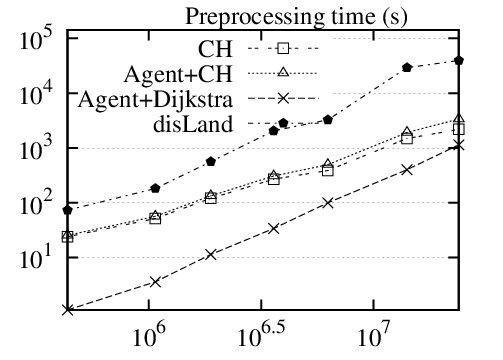


Exp-4: Preprocessing time and space overhead. In the fourth set of experiments, we tested the space cost and preprocessing time of Dijkstra, Agent + Dijkstra, ch, Agents + ch, arcFlag, Agents + arcFlag, and disLand. For disLand, we did a second level partition on the super graphs into fragments, determined as follows: if ¿ , and , otherwise, where is the number of fragments of the shrink graphs, shown in Table 4. arcFlag called Metis to partition the graphs into fragments as well. The results are reported in Figure 8.
The results tell us that (1) the space cost follows the order: arcFlag Agents + arcFlag disLand Agents + ch Agent + Dijkstra Dijkstra ch; and (2) the preprocessing time follows the order: arcFlag Agents + arcFlag disLand Agents + ch ch Agent + Dijkstra. In particular, ch even uses less space than the original graphs, and disLand uses about time extra space, while Agent + arcFlag and arcFlag use and times extra space, respectively. While ch and disLand could finish the preprocessing in less than and hours, repectively, it took Agent + arcFlag and arcFlag and hours, respectively. Thus all approaches, except arcFlag and Agents + arcFlag, produce auxiliary structures with a small space cost and in a reasonably fast way.
Exp-5: Efficiency of shortest distance queries. In the last set of experiments, using the sets of distance queries, we tested the efficiency of Dijkstra, Agent + Dijkstra, ch, Agents + ch, arcFlag, Agents + arcFlag, and disLand on the datasets with corresponding generated auxiliary structures. The results are reported in Figures 9 and 10. As for all algorithms, their counterparts with agents were always faster, we omitted their running time for clarity.
The results tell us that (1) all algorithms scale well w.r.t. the graph sizes and w.r.t. the distance queries, and (2) the efficiency of the algorithms follows the order: disLand, Agent + ch Agent + arcFlag Agent + Dijkstra. For the distance queries () with relative close distance node pairs, the running time of disLand and Agent + ch is comparable. However, for the distance queries () with relative long distance node pairs, disLand is apparently faster than Agent + ch. Indeed, for on the US dataset, disLand is , , , , and times faster than Dijkstra, Agent + Dijkstra, arcFlag, Agent + arcFlag, ch, and Agent + ch, respectively.
Summary. From these experimental results, we find the following. (1) disLand scales well on large road graphs, e.g., it takes only seconds on graphs with nodes and edges. (2) Agents and their dras are a light-weight preprocessing technique, which benefits almost all shortest distance algorithms. (3) Agents, graph partitions and hybrid landmark covers together provide a good solution to produce small super graphs, which typically have 2–4% nodes and 10–15% edges compared with the original graphs. (4) disLand produces auxiliary structures with a small space cost (about of the input graphs), and their preprocessing could be finished in a reasonably fast way. (5) disLand provides a good solution for shortest distance query answering, especially for far node pairs on large graphs. For on the US dataset, it is even times faster than Agent + ch, where ch is the best approach without using extra information, e.g., longitude and latitude, tested in [34]. Finally, (6) hybrid landmark covers play a central role that makes our proposed techniques (e.g., agents and graph partitions) and the existing techniques (e.g., ch and arcFlag) seamlessly integrate into a unified framework – disLand.
VIII Conclusion
We have studied how to apply distance landmarks for fast exact shortest distance query answering on large weighted undirected road graphs. To our knowledge, we are among the first to settle this problem. We have shown that the direct application of distance landmarks is impractical due to their high space and time cost. To rectify these problems, we have proposed: hybrid landmark covers, agents and dras, bounded graph partitions, super graphs and framework disLand. We have also verified, both analytically and experimentally, that hybrid landmark covers, together with these techniques, significantly improve efficiency of shortest distance queries.
Several topics are targeted for future work. We are to extend our techniques for other types real-life datasets that could be modeled as weighted undirected graphs, e.g., social networks. We are also to explore the possibility of applying distance landmarks for other classes of graph queries, e.g., reachability.
References
- [1] I. Abraham, D. Delling, A. V. Goldberg, and R. F. F. Werneck. A hub-based labeling algorithm for shortest paths in road networks. In SEA, 2011.
- [2] A. Z. Broder, R. Kumar, F. Maghoul, P. Raghavan, S. Rajagopalan, R. Stata, A. Tomkins, and J. L. Wiener. Graph structure in the web. Computer Networks, 33(1-6):309–320, 2000.
- [3] CH. http://algo2.iti.kit.edu/english/routeplanning.php.
- [4] E. P. F. Chan and H. Lim. Optimization and evaluation of shortest path queries. VLDB J., 16(3):343–369, 2007.
- [5] J. Cheng, Y. Ke, S. Chu, and C. Cheng. Efficient processing of distance queries in large graphs: a vertex cover approach. In SIGMOD, 2012.
- [6] T. H. Cormen, C. E. Leiserson, R. L. Rivest, and C. Stein. Introduction to Algorithms. The MIT Press, 2001.
- [7] E. W. Dijkstra. A note on two problems in connexion with graphs. Numerische Mathematik, 1:269–271, 1959.
- [8] DIMACS. http://www.dis.uniroma1.it/challenge9.
- [9] M. Franceschet. Collaboration in computer science: A network science approach. JASIST, 62(10):1992–2012, 2011.
- [10] M. L. Fredman and R. E. Tarjan. Fibonacci heaps and their uses in improved network optimization algorithms. In FOCS, 1984.
- [11] Full version. http://mashuai.buaa.edu.cn/full.pdf.
- [12] M. Garey and D. Johnson. Computers and Intractability: A Guide to the Theory of NP-Completeness. W. H. Freeman and Company, 1979.
- [13] R. Geisberger, P. Sanders, D. Schultes, and D. Delling. Contraction hierarchies: Faster and simpler hierarchical routing in road networks. In WEA, 2008.
- [14] A. V. Goldberg and C. Harrelson. Computing the shortest path: A* search meets graph theory. In SODA, 2005.
- [15] J. E. Hopcroft and R. E. Tarjan. Efficient algorithms for graph manipulation [h] (algorithm 447). Commun. ACM, 16(6):372–378, 1973.
- [16] G. Karypis and V. Kumar. A fast and high quality multilevel scheme for partitioning irregular graphs. SISC, 20(1):359–392, 1998.
- [17] B. W. Kernighan and S. Lin. An efficientheuristic procedure for partitioning graphs. Bell System Technical Journal, 49(1):13–21, 1970.
- [18] T. Lappas, K. Liu, and E. Terzi. Finding a team of experts in social networks. In KDD, 2009.
- [19] J. Leskovec, K. J. Lang, A. Dasgupta, and M. W. Mahoney. Statistical properties of community structure in large social and information networks. In WWW, 2008.
- [20] M. Luby and P. Ragde. A bidirectional shortest-path algorithm with good average-case behavior. Algorithmica, 4(4):551–567, 1989.
- [21] Metis. http://glaros.dtc.umn.edu/gkhome/views/metis.
- [22] R. H. Möhring, H. Schilling, B. Schütz, D. Wagner, and T. Willhalm. Partitioning graphs to speedup Dijkstra’s algorithm. ACM Journal of EA, 11, 2006.
- [23] S. Mozes and C. Sommer. Exact distance oracles for planar graphs. In SODA, 2012.
- [24] M. Potamias, F. Bonchi, C. Castillo, and A. Gionis. Fast shortest path distance estimation in large networks. In CIKM, 2009.
- [25] P. Sanders and D. Schultes. Highway hierarchies hasten exact shortest path queries. In ESA, 2005.
- [26] J. Sankaranarayanan and H. Samet. Query processing using distance oracles for spatial networks. TKDE, 22(8):1158–1175, 2010.
- [27] J. Sankaranarayanan, H. Samet, and H. Alborzi. Path oracles for spatial networks. PVLDB, 2(1), 2009.
- [28] A. D. Sarma, S. Gollapudi, M. Najork, and R. Panigrahy. A sketch-based distance oracle for web-scale graphs. In WSDM, 2010.
- [29] S. Saunders and T. Takaoka. Solving shortest paths efficiently on nearly acyclic directed graphs. TCS, 370(1-3):94–109, 2007.
- [30] M. Thorup and U. Zwick. Approximate distance oracles. J. ACM, 52(1):1–24, 2005.
- [31] V. V. Vazirani. Approximation Algorithms. Springer, 2003.
- [32] D. Wagner and T. Willhalm. Speed-up techniques for shortest-path computations. In STACS, 2007.
- [33] F. Wei. Tedi: efficient shortest path query answering on graphs. In SIGMOD, 2010.
- [34] L. Wu, X. Xiao, D. Deng, G. Cong, A. D. Zhu, and S. Zhou. Shortest path and distance queries on road networks: An experimental evaluation. PVLDB, 5(5), 2012.
- [35] S. Yang, X. Yan, B. Zong, and A. Khan. Towards effective partition management for large graphs. In SIGMOD, 2012.