On a Duality Between Recoverable Distributed Storage and Index Coding

Arya Mazumdar Affiliation: Department of ECE
University of Minnesota– Twin Cities
Minneapolis, MN 55455
email: arya@umn.edu

Abstract

In this paper, we introduce a model of a single-failure locally recoverable distributed storage system. This model appears to give rise to a problem seemingly dual of the well-studied index coding problem. The relation between the dimensions of an optimal index code and optimal distributed storage code of our model has been established in this paper. We also show some extensions to vector codes.

I Introduction

Recently, local repair property of error-correcting codes is the center of a lot of research activity. In a distributed storage system, a single server failure is the most common error-event, and in that case, the aim is to reconstruct the content of the server from as few other servers as possible (or by downloading minimal amount of data from other servers). The study of such regenerative storage systems was initiated in [9] and then followed up in several recent works. In [11], a particularly neat characterization of a local repair property is provided. It is assumed that, each symbol of an encoded message is stored at a different node in the network (since the symbol alphabet is unconstrained, a symbol could represent a packet or block of bits of arbitrary size). Accordingly, [11] investigates codes allowing any single symbol of any codeword to be recovered from at most a constant number of other symbols of the codeword, i.e., from a number of symbols that does not grow with the length of the code.

The work of [11] is then further generalized to several directions and a number of impossibility results regarding, as well as construction of, locally repairable codes were presented (see, for example, [17, 22, 5, 20, 12]), culminating in very recent construction of [21].

However, the topology of the network of distributed storage system is missing from the above definition of local repairability. Namely, all servers are treated equally irrespective of their physical positions, proximities, and connections. Here we take a step to include that into consideration. We study the case when the topology of the storage system is fixed and the network of storage is given by a graph. In our model, the servers are represented by the vertices of a graph, and two servers are connected by an edge if it is easier to establish up-or-down link between them, for reasons such as physical locations of the servers, architecture of the distributed system or homogeneity of softwares, etc. It turns out that, our model is closely related to the following index coding problem on a side information graph. In this paper, we formalize this relation.

I-A Index Coding

A very natural “source coding” problem on a network, called the index coding, was introduced in [3], and since then is a subject of extensive research. In the index coding problem a side information graph $G(V,E)$ is given. Each vertex $v\in V$ represents a receiver that is interested in knowing a uniform random variable $Y_{v}\in{\mathbb{F}}_{q}$ . For any $v\in V$ , define $N(v)=\{u\in V:(v,u)\in E\}$ to be the neighborhood of $v$ . The receiver at $v$ knows the values of the variables $Y_{u},u\in N(v)$ . How much information should a broadcaster transmit, such that every receiver knows the value of its desired random variable? Let us give the formal definition from [3], adapted for $q$ -ary alphabet here.

Definition 1

An index code ${\mathcal{C}}$ for ${\mathbb{F}}_{q}^{n}$ with side information graph $G(V,E),V=\{1,2,\dots,n\},$ is a set of codewords in ${\mathbb{F}}_{q}^{\ell}$ together with:

1.

An encoding function $f$ mapping inputs in ${\mathbb{F}}_{q}^{n}$ to codewords, and
2.

A set of deterministic decoding functions $g_{1},\dots,g_{n}$ such that $g_{i}\Big(f(Y_{1},\dots,Y_{n}),\{Y_{j}:j\in N(i)\}\Big)=Y_{i}$ for every $i=1,\dots,n$ .

The encoding and decoding functions depend on G. The integer $\ell$ is called the length of ${\mathcal{C}}$ , or $\mathrm{len}({\mathcal{C}})$ . Given a graph $G$ the minimum possible length of an index code is denoted by $\mathrm{INDEX}_{q}(G)$ .

In [3], a connection has been made with the length of an index code to a quantity called the minrank of the graph. Suppose, $A=(a_{ij})$ be an $n\times n$ matrix over ${\mathbb{F}}_{q}$ . It is said that $A$ fits $G(V,E)$ over ${\mathbb{F}}_{q}$ if $a_{ii}\neq 0$ for all $i$ and $a_{ij}=0$ whenever $(i,j)\notin E$ and $i\neq j$ .

Definition 2

The minrank of a graph $G(V,E)$ over ${\mathbb{F}}_{q}$ is defined to be,

\mathrm{minrank}_{q}(G)=\min\{\rank_{{\mathbb{F}}_{q}}(A):A\text{ fits }G\}.

(1)

It was shown in [3], that,

\mathrm{INDEX}_{q}(G)\leq\mathrm{minrank}_{q}(G),

(2)

and indeed, $\mathrm{minrank}_{q}(G)$ is the minimum length of an index code on $G$ when the encoding function, and the decoding functions are all linear. The above inequality can be strict in many cases [1, 14].

In [1], the problem of index coding is further generalized. We only describe here what is important for our context. Just for this part, assume $q=2$ . To characterize the optimal size of an index code, [1] introduces the notion of a confusion graph. Two input strings, ${\boldsymbol{x}}=(x_{1},\dots,x_{n}),{\boldsymbol{y}}=(y_{1},\dots,y_{n})\in{\mathbb{F}}_{2}^{n}$ are called confusable if there exists some $i\in\{1,\dots,n\}$ , such that $x_{i}\neq y_{i}$ , but $x_{j}=y_{j},$ for all $j\in N(i)$ . In the confusion graph of $G$ , total number of vertices are $2^{n}$ , and each vertex represents a different $\{0,1\}$ -string of length $n$ . There exists an edge between two vertices if and only if the corresponding two strings are confusable with respect to the graph $G$ . The maximum size of an independent set of the confusion graph is denoted by $\gamma(G)$ .

However, the confusion graph and $\gamma(G)$ in [1] were used as tools to characterize the the rate of index coding; they were not used to model any immediate practical problem. In this paper, we show that, this notion of confusable strings fits perfectly to the situation of local recovery of a distributed storage system. Namely, $\gamma(G)$ , in our problem becomes the largest possible size of a locally recoverable code for a system with topology given by $G$ .

I-B Organization

The paper is organized in the following way. In Section II, we introduce formally the model of a recoverable distributed storage system. The notion of an optimal recoverable distributed storage code given a graph and its relation to the optimal index code is also described here. In Section III, we provide an algorithmic proof of the main duality relation of the index code and distributed storage code. Our proof is based on a covering argument of the Hamming space, and rely on the fact that for any given subset of the Hamming space there exists a translation of the set, that has very small overlap with the original subset. We conclude with an extension of the duality theorem to vector codes and a remark on the optimal linearly recoverable distributed storage codes¹¹ 1 After the first version of this paper appeared in arxiv, we were made aware of a parallel independent work [19] where for vector linear codes the duality between RDSS and index codes (see the discussion preceding Eq. (4)) is proved. The authors of [19] use that observation to give an upper bound on the optimal linear sum rate of the multiple unicast network coding problem. In this paper we have a different focus: we show a proof of (approximate) duality for general (nonlinear) codes..

II Recoverable distributed storage systems

Consider the network of distributed storage, for example, one of Fig. 1. As mentioned in the introduction, the property of two servers connected by an edge is based on the ease of establishing a link between the servers. It is also possible (and sensible, perhaps) to model this as a directed graph (especially when uplink and downlink constructions have varying difficulties). In the following, we assume that the graph is directed, and an undirected graph is just a special case.

If the data of any one server is lost, we want to recover it from the nearby servers, i.e., the ones with which it is easy to establish a link. This notion is formalized below.

Suppose, the directed graph $G(V,E)$ represents the network of storage. Each element of $V$ represents a server, and in the case of a server failure (say, $v\in V$ is the failed server) one must be able to reconstruct its content from its neighborhood $N(v)$ .

Given, this constraint what is the maximum amount of information one can store in the system? Without loss of generality, assume $V=\{1,2,\dots,n\}$ and the variables $X_{1},X_{2},\dots,X_{n}$ respectively denote the content of the vertices, where, $X_{i}\in{\mathbb{F}}_{q},i=1,\dots,n.$

Definition 3

A recoverable distributed storage system (RDSS) code ${\mathcal{C}}\subseteq{\mathbb{F}}_{q}^{n}$ with storage recovery graph $G(V,E),V=\{1,2,\dots,n\},$ is a set of vectors in ${\mathbb{F}}_{q}^{n}$ together with:

-

A set of deterministic recovery functions, $f_{i}:{\mathbb{F}}_{q}^{|N(i)|}\to{\mathbb{F}}_{q}$ for $i=1,\dots,n$ such that for any codeword $(X_{1},X_{2},\dots,X_{n})\in{\mathbb{F}}_{q}^{n},$

$X_{i}=f_{i}(\{X_{j}:j\in N(i)\}),\quad i=1,\dots,n.$ (3)

Again, the decoding functions depend on G. The log-size of the code, $\log_{q}|{\mathcal{C}}|$ , is called the dimension of ${\mathcal{C}}$ , or $\dim({\mathcal{C}})$ . Given a graph $G$ the maximum possible dimension of an RDSS code is denoted by $\mathrm{RDSS}_{q}(G)$ .

Refer to caption — Fig. 1: Example of a distributed storage graph

For example, consider the graph of Fig. 1 again. Here, $V=\{1,2,3,4,5\}$ . The recovery sets of each vertex (or storage nodes) are given by:

	$\displaystyle N(1)=\{2,3,4,5\},\,N(2)=\{1,3\},N(3)=\{1,2,4\},$
	$\displaystyle N(4)=\{1,3,5\},N(5)=\{1,4\}.$

Suppose, the contents of the nodes $1,2,\dots,5$ are $X_{1},X_{2},\dots,X_{5}$ respectively, where, $X_{i}\in{\mathbb{F}}_{q},i=1,\dots,5.$ Moreover, $X_{1}=f_{1}(X_{2},X_{3},X_{4},X_{5}),X_{2}=f_{2}(X_{1},X_{3}),X_{3}=f_{3}(X_{1},X_{2},X_{4}),X_{4}=f_{4}(X_{1},X_{3},X_{5}),X_{5}=f_{5}(X_{1},X_{4}).$

Assume, the functions $f_{i},i=1,\dots,5$ , in this example are linear. That is, for $\alpha_{ij}\in{\mathbb{F}}_{q},1\leq i,j\leq 5,$

	$\displaystyle X_{1}$	$\displaystyle=\alpha_{12}X_{2}+\alpha_{13}X_{3}+\alpha_{14}X_{4}+\alpha_{15}X_{5}$
	$\displaystyle X_{2}$	$\displaystyle=\alpha_{21}X_{1}+\alpha_{23}X_{3}$
	$\displaystyle X_{3}$	$\displaystyle=\alpha_{31}X_{1}+\alpha_{32}X_{2}+\alpha_{34}X_{4}$
	$\displaystyle X_{4}$	$\displaystyle=\alpha_{41}X_{1}+\alpha_{43}X_{3}+\alpha_{45}X_{5}$
	$\displaystyle X_{5}$	$\displaystyle=\alpha_{51}X_{1}+\alpha_{54}X_{4}.$

This implies, $(X_{1},X_{2},\dots,X_{5})$ must belong to the null-space (over ${\mathbb{F}}_{q}$ ) of

D\equiv\left(\begin{array}[]{ccccc}1&-\alpha_{12}&-\alpha_{13}&-\alpha_{14}&-\alpha_{15}\\ -\alpha_{21}&1&-\alpha_{23}&0&0\\ -\alpha_{31}&-\alpha_{32}&1&-\alpha_{34}&0\\ -\alpha_{41}&0&-\alpha_{43}&1&-\alpha_{45}\\ -\alpha_{51}&0&0&-\alpha_{54}&1\end{array}\right).

The dimension of the null-space of $D$ is $n$ minus the rank of $D$ . Hence, it is evident that the dimension of the RDSS code is $n-\mathrm{minrank}_{q}(G)$ . Also, the null-space of a linear index code for $G$ is a linear RDSS code for the same graph $G$ (see, Eq. (2)). From the above discussion, we have,

\mathrm{RDSS}_{q}(G)\geq n-\mathrm{minrank}_{q}(G),

(4)

and, $n-\mathrm{minrank}_{q}(G)$ is the maximum possible dimension of an RDSS code when the recovery functions are all linear. At this point, it is tempting to make the assertion $\mathrm{RDSS}_{q}(G)=n-\mathrm{INDEX}_{q}(G)$ , however, that would be wrong. This is shown in the following example.

This example is present in [1], and the distributed storage graph, a pentagon, is shown in Fig. 2. For this graph, a maximum-sized binary RDSS code consists of the codewords $\{00000,01100,00011,11011,11101\}$ . The recovery functions are given by,

	$\displaystyle X_{1}=X_{2}\wedge X_{5},X_{2}=X_{1}\vee X_{3},X_{3}=X_{2}\wedge\bar{X}_{4},$
	$\displaystyle X_{4}=\bar{X}_{3}\wedge X_{5}X_{5}=X_{1}\vee X_{4}.$

If all the recovery functions are linear, we could not have an RDSS code with so many codewords. Here $\mathrm{RDSS}_{2}(G)=\log_{2}5$ . On the other hand, the minimum length of an index code for this graph is $3$ , i.e., $\mathrm{INDEX}_{2}(G)=3$ , and this is achieved by the following linear mappings. The broadcaster transmit $Y_{1}=X_{2}+X_{3},Y_{2}=X_{4}+X_{5}$ and $Y_{3}=X_{1}+X_{2}+X_{3}+X_{4}+X_{5}.$ The decoding functions are, $X_{1}=Y_{1}+Y_{2}+Y_{3};X_{2}=Y_{1}+X_{3};X_{3}=Y_{1}+X_{2};X_{4}=Y_{2}+X_{5};X_{5}=Y_{2}+X_{4}.$

Although in general $\mathrm{RDSS}_{q}(G)\neq n-\mathrm{INDEX}_{q}(G)$ , these two quantities are not too far from each other. In particular, for large enough alphabet, the left and right hand sides can be arbitrarily close. This is reflected in Thm. 1 below.

It is to be noted that, we refrain from using ceiling and floor functions for clarity in this paper. In many cases, it is clear that the number of interest is not an integer and should be rounded off to the nearest larger or smaller integer. The main results do not change for this.

II-A Implication of the results of [1]

The result of [1] can be cast in our context in the following way.

Theorem 1

Given a graph $G(V,E)$ , we must have,

	$\displaystyle n-$	$\displaystyle\mathrm{RDSS}_{q}(G)\leq\mathrm{INDEX}_{q}(G)\leq n-\mathrm{RDSS}_{q}(G)$
		$\displaystyle+\log_{q}\Big(\min\{n\ln q,1+\mathrm{RDSS}_{q}(G)\ln q\}\Big).$		(5)

This result is purely graph-theoretic, the way it was presented in [1]. In particular, the size of maximum independent set of the confusion graph, $\gamma(G)$ was identified as the size of the RDSS code, and its relation to the chromatic number of the confusion graph, which represents the size of the index code was found. Namely the proof was dependent on the following two crucial steps.

1.

The chromatic number of the graph can only be so much away from the fractional chromatic number (see, [1] for detailed definition).
2.

The confusion graph is vertex transitive. This implies that the maximum size of an independent set is equal to the number of vertices divided by the fractional chromatic number.

A proof of the first fact above can be found in [13]. In what follows, we give a simple coding theoretic proof of this main theorem, without using the notion of the confusion graph or its vertex transitivity, for completeness.

III The proof of the duality

We prove Theorem 1 with the help of following two lemmas. The first of them is immediate.

Lemma 2

If there exists an index code ${\mathcal{C}}$ of length $\ell$ for a side information graph $G$ on $n$ vertices, then there exists an RDSS code of dimension $n-\ell$ for the distributed storage graph $G$ .

Proof:

Suppose, the encoding and decoding functions of the index code ${\mathcal{C}}$ are $f:{\mathbb{F}}_{q}^{n}\to{\mathbb{F}}_{q}^{\ell}$ and $g_{i}:{\mathbb{F}}_{q}^{\ell+N(i)}\to{\mathbb{F}}_{q},i=1,\dots,n$ . There must exists some ${\boldsymbol{x}}\in{\mathbb{F}}_{q}^{\ell}$ such that $|\{{\boldsymbol{y}}\in{\mathbb{F}}_{q}^{n}:f({\boldsymbol{y}})={\boldsymbol{x}}\}|\geq q^{n-\ell}$ . Let, ${\mathcal{D}}_{\boldsymbol{x}}\equiv\{{\boldsymbol{y}}\in{\mathbb{F}}_{q}^{n}:f({\boldsymbol{y}})={\boldsymbol{x}}\}$ be the distributed storage code with recovery functions, f_i({X_j, j ∈N(i)}) ≡g_i(x, {X_j, j ∈N(i)}). ∎The second lemma is the more interesting one.

Lemma 3

If there exists an RDSS code ${\mathcal{C}}$ of dimension $k$ for a distributed storage graph $G$ on $n$ vertices, then there exists an index code of length $n-k+\log_{q}\min\{n\ln q,1+k\ln q\}$ for the side information graph $G$ .

To prove this result, we need the help of a number of other lemmas. First of all notice that, translation of any RDSS code is an RDSS code.

Lemma 4

Suppose, ${\mathcal{C}}\subseteq{\mathbb{F}}_{q}^{n}$ is an RDSS code. Then any known translation of ${\mathcal{C}}$ is also an RDSS code of same dimension. That is, for any ${\boldsymbol{a}}\in{\mathbb{F}}_{q}^{n}$ , ${\mathcal{C}}+{\boldsymbol{a}}\equiv\{{\boldsymbol{y}}+{\boldsymbol{a}}:{\boldsymbol{y}}\in{\mathcal{C}}\}$ is an RDSS code of dimension $\log_{q}|{\mathcal{C}}|$ .

Proof:

Let, $(X_{1},\dots,X_{n})\in{\mathcal{C}}.$ Also assume, ${\boldsymbol{a}}=(a_{1},\dots,a_{n})$ , and $X^{\prime}_{i}=X_{i}+a_{i}$ . We know that, there exist recovery functions such that, $X_{i}=f_{i}(\{X_{j}:j\in N(i)\}).$

Now, $X^{\prime}_{i}=X_{i}+a_{i}=f_{i}(\{X_{j}:j\in N(i)\})+a_{i}\equiv f^{\prime}_{i}(\{X^{\prime}_{j}:j\in N(i)\}$ . ∎

In particular, Lemma 3 crucially use the existence of a covering of the entire ${\mathbb{F}}_{q}^{n}$ , by translations of an RDSS code.

Proof:

We will show that there exists, ${\mathcal{C}}_{1},\dots,{\mathcal{C}}_{m},$ ${\mathcal{C}}_{i}\in{\mathbb{F}}_{q}^{n},i=1,\dots,m,$ all of which are RDSS codes of dimension $k$ such that

\cup_{i=1}^{m}{\mathcal{C}}_{i}={\mathbb{F}}_{q}^{n},

(6)

where $m=q^{n-k}\min\{n\ln q,1+k\ln q\}$ . Assume, the above is true. Then, any ${\boldsymbol{y}}\in{\mathbb{F}}_{q}^{n}$ must belong to at least one of the $C_{i}$ s. Suppose, ${\boldsymbol{y}}\equiv(Y_{1},\dots,Y_{n})\in{\mathbb{F}}_{q}^{n}$ and ${\boldsymbol{y}}\in C_{i}$ . Then, the encoding function of the desired index code ${\mathcal{D}}$ is simply given by, $f({\boldsymbol{y}})=i$ . If the recovery functions of ${\mathcal{C}}_{i}$ are $f^{i}_{j},j=1,\dots,n$ , then, the decoding functions of ${\mathcal{D}}$ are given by: g_j(i, {Y_l: l ∈N(j)}) = f^i_j({Y_l: l ∈N(j)}). Clearly the length of the index code is $\log_{q}m=n-k+\log_{q}(\min\{n\ln q,1+k\ln q\})$ .

It remains to show the existence of RDSS codes ${\mathcal{C}}_{1},\dots,{\mathcal{C}}_{m}$ of dimension $k$ each with property (6). We will show that, there exists $m$ vectors ${\boldsymbol{x}}_{j},j=1,\dots,m$ such that

{\mathcal{C}}_{i}={\mathcal{C}}+{\boldsymbol{x}}_{i}\equiv\{{\boldsymbol{y}}+{\boldsymbol{x}}_{i}:{\boldsymbol{y}}\in{\mathcal{C}}\}.

(7)

From Lemma 4, ${\mathcal{C}}_{i},i=1,\dots,m$ are all RDSS codes of dimension $k$ . Suppose, ${\boldsymbol{x}}_{i},i=1,\dots,m$ are randomly and independently chosen from ${\mathbb{F}}_{q}^{n}$ . Now, Pr(∪_i =1^m’ C_i ≠F_q^n) ≤q^n (1-—C—/q^n)^m’ ¡ q^n e^-m’—C—/q^n ≤1, when we set $m^{\prime}=q^{n-k}n\ln q\leq m$ in the above expression (see [2, Prop. 3.12]).

If, instead we set $m^{\prime}=q^{n-k}k\ln q$ then, $\Pr(\cup_{i=1}^{m^{\prime}}{\mathcal{C}}_{i}\neq{\mathbb{F}}_{q}^{n})\leq q^{n-k}$ , which is also the expected number of points, that do not belong to any of the $m^{\prime}$ translations. To cover all these remaining points we need at most $q^{n-k}$ other transmission. Hence, there must exists a covering such that $q^{n-k}k\ln q+q^{n-k}=q^{n-k}(k\ln q+1)\leq m$ translations suffice. ∎

The proof of Lemma 3 can also be given via a greedy algorithm. In the greedy algorithm about $\log m$ vectors are recursively chosen instead of $m$ random vectors. We provide the construction/proof next.

III-A A greedy algorithm for the proof of Lemma 3

Note that, to proof Lemma 3 we need to show the existence of a covering of the entire ${\mathbb{F}}_{q}^{n}$ , by translations of an RDSS code. What we show here is that the translations themselves form a linear subspace. The greedy covering argument that we employ below was used to show the existence of good linear covering codes in [8] (see, also, [10, 7]), and was reintroduced in [15] to show the existence of balancing sets.

Lemma 5 (Bassalygo-Elias)

Suppose, ${\mathcal{C}},{\mathcal{B}}\subseteq{\mathbb{F}}_{q}^{n}.$ Then,

\sum_{{\boldsymbol{x}}\in{\mathbb{F}}_{q}^{n}}\mid({\mathcal{C}}+{\boldsymbol{x}})\cap{\mathcal{B}}\mid=|{\mathcal{C}}||{\mathcal{B}}|.

(8)

Proof:

	$\displaystyle\sum_{{\boldsymbol{x}}\in{\mathbb{F}}_{q}^{n}}\mid({\mathcal{C}}+{\boldsymbol{x}})\cap{\mathcal{B}}\mid$	$\displaystyle=\|\{({\boldsymbol{x}},{\boldsymbol{y}}):{\boldsymbol{x}}\in{\mathbb{F}}_{q}^{n},{\boldsymbol{y}}\in{\mathcal{B}},{\boldsymbol{y}}\in{\mathcal{C}}+{\boldsymbol{x}}\}\|$
		$\displaystyle=\|\{({\boldsymbol{x}},{\boldsymbol{y}}):{\boldsymbol{x}}\in{\mathbb{F}}_{q}^{n},{\boldsymbol{y}}\in{\mathcal{B}},{\boldsymbol{x}}\in{\boldsymbol{y}}-{\mathcal{C}}\}\|$
		$\displaystyle=\|\{({\boldsymbol{x}},{\boldsymbol{y}}):{\boldsymbol{y}}\in{\mathcal{B}},{\boldsymbol{x}}\in{\boldsymbol{y}}-{\mathcal{C}}\}\|$
		$\displaystyle=\|{\mathcal{B}}\|\|{\boldsymbol{y}}-{\mathcal{C}}\|=\|{\mathcal{C}}\|\|{\mathcal{B}}\|,$

where ${\boldsymbol{y}}-{\mathcal{C}}\equiv\{{\boldsymbol{y}}-{\boldsymbol{a}}:{\boldsymbol{a}}\in{\mathcal{C}}\}$ . ∎For any set ${\mathcal{F}}\subseteq{\mathbb{F}}_{q}^{n}$ , define

Q({\mathcal{F}})\equiv 1-\frac{|{\mathcal{F}}|}{q^{n}}.

(9)

In words, $Q({\mathcal{F}})$ denote the proportion of ${\mathbb{F}}_{q}^{n}$ that is not covered by ${\mathcal{F}}$ . The following property is a result of Lemma 5.

Lemma 6

For every subset ${\mathcal{F}}\subseteq{\mathbb{F}}_{q}^{n}$ ,

q^{-n}\sum_{{\boldsymbol{x}}\in{\mathbb{F}}_{q}^{n}}Q({\mathcal{F}}\cup({\mathcal{F}}+{\boldsymbol{x}}))=Q({\mathcal{F}})^{2}.

(10)

Proof:

We have, —F∪(F+x)— = 2—F— - —F∩(F+x)—. Therefore, Q(F∪(F+x)) = 1 - 2—F— q^-n + —F∩(F+x)—q^-n, and hence,

	$\displaystyle q^{-n}\sum_{{\boldsymbol{x}}\in{\mathbb{F}}_{q}^{n}}Q({\mathcal{F}}\cup({\mathcal{F}}+{\boldsymbol{x}}))$	$\displaystyle=1-2\|{\mathcal{F}}\|q^{-n}$
		$\displaystyle\quad+q^{-2n}\sum_{{\boldsymbol{x}}\in{\mathbb{F}}_{q}^{n}}\|{\mathcal{F}}\cap({\mathcal{F}}+{\boldsymbol{x}})\|$
		$\displaystyle=1-2\|{\mathcal{F}}\|q^{-n}+q^{-2n}\|{\mathcal{F}}\|^{2}$
		$\displaystyle=(1-\|{\mathcal{F}}\|q^{-n})^{2},$

where in the second line we have used Lemma 5. ∎

The implication of the above lemma is the following result.

Lemma 7

For every subset ${\mathcal{F}}\subseteq{\mathbb{F}}_{q}^{n}$ , there exists $m=q^{n}|{\mathcal{F}}|^{-1}\min\{n\ln q,1+\ln|{\mathcal{F}}|\}$ vectors ${\boldsymbol{x}}_{0}=0,{\boldsymbol{x}}_{1},{\boldsymbol{x}}_{2},\dots,{\boldsymbol{x}}_{m-1}\in{\mathbb{F}}_{q}^{n}$ , such that

\cup_{i=0}^{m-1}({\mathcal{F}}+{\boldsymbol{x}}_{i})={\mathbb{F}}_{q}^{n}.

Proof:

From Lemma 6, for every subset ${\mathcal{F}}\subseteq{\mathbb{F}}_{q}^{n}$ , there exists ${\boldsymbol{x}}\in{\mathbb{F}}_{q}^{n}$ such that Q(F∪(F+x)) ≤Q(F)^2. For the set ${\mathcal{F}}\equiv{\mathcal{F}}_{0}$ , recursively define, for i =1, 2,… F_i = F_i-1 ∪(F_i-1 + z_i-1), where ${\boldsymbol{z}}_{i}\in{\mathbb{F}}_{q}^{n}$ is such that, Q(F_i∪(F_i+z_i)) ≤Q(F_i)^2, i =0,1,… Clearly, Q(F_t) ≤Q(F_0)^2^t = (1- q^-n —F—)^2^t ≤e^- q^-n —F—2^t. At this point we can just use the argument at the end of proof of Lemma 3, with $2^{t}$ plating the role of $m^{\prime}$ .

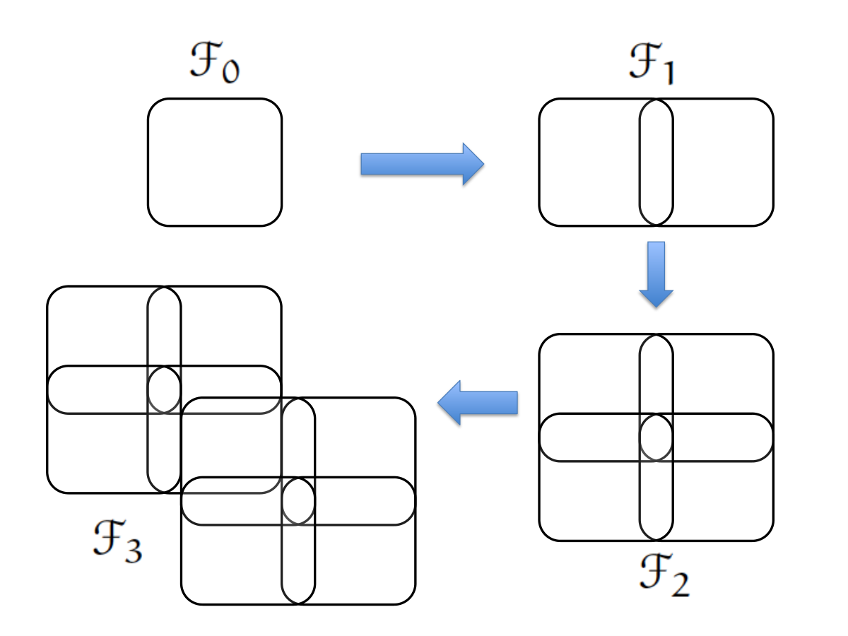
On the other hand ${\mathcal{F}}_{t}$ contains ${\mathcal{F}}_{0}$ and its $2^{t}-1$ translations (see, Figure 3 for an illustration). Hence, there exists $m=\min\Big\{\frac{q^{n}n\ln q}{|{\mathcal{F}}|},\frac{q^{n}(1+\ln|{\mathcal{F}}|)}{|{\mathcal{F}}|}\Big\}$ vectors ${\boldsymbol{x}}_{0}=0,{\boldsymbol{x}}_{1},{\boldsymbol{x}}_{2},\dots,{\boldsymbol{x}}_{m-1}\in{\mathbb{F}}_{q}^{n}$ , such that ∪_i=0^m-1 (F+x_i) = F_q^n.

∎

To complete the proof of Lemma 3, as before, we just show the existence of RDSS codes ${\mathcal{C}}_{0}\equiv{\mathcal{C}},{\mathcal{C}}_{1},\dots,{\mathcal{C}}_{m-1}$ of dimension $k$ each with property (6). This is achieved by choosing $m-1$ vectors ${\boldsymbol{x}}_{j},j=1,\dots,m-1$ such that

{\mathcal{C}}_{i}={\mathcal{C}}+{\boldsymbol{x}}_{i}\equiv\{{\boldsymbol{y}}+{\boldsymbol{x}}_{i}:{\boldsymbol{y}}\in{\mathcal{C}}\}.

(11)

From Lemma 4, ${\mathcal{C}}_{i},i=1,\dots,m-1$ are all RDSS codes of dimension $k$ . Moreover, from Lemma 7, we already know the existence of ${\boldsymbol{x}}_{j},j=1,\dots,m-1$ such that property (6) is satisfied. However, from Lemma 7 it is also clear that these $m$ vectors form a linear subspace and can be generated by only $\log_{q}m$ vectors.

Corollary 8

For every subset ${\mathcal{F}}\subseteq{\mathbb{F}}_{q}^{n}$ , there exists a linear subspace ${\mathcal{D}}\in{\mathbb{F}}_{q}^{n}$ such that $|{\mathcal{D}}|=q^{n}|{\mathcal{F}}|^{-1}n\ln q$ and

\cup_{{\boldsymbol{x}}\in{\mathcal{D}}}({\mathcal{F}}+{\boldsymbol{x}})={\mathbb{F}}_{q}^{n}.

The above result is helpful in the decoding process of the index code. If ${\mathcal{C}}$ is an RDSS code and ${\mathcal{D}}$ is the linear subspace such that $\cup_{{\boldsymbol{x}}\in{\mathcal{D}}}({\mathcal{C}}+{\boldsymbol{x}})={\mathbb{F}}_{q}^{n}$ , then the decoding of the obtained index code can be performed from ${\boldsymbol{x}}\in{\mathbb{F}}_{q}^{\log_{q}|{\mathcal{D}}|}$ by first multiplying ${\boldsymbol{x}}$ with the generator matrix of ${\mathcal{D}}$ and then shifting ${\mathcal{C}}$ by it. Hence, if there is a polynomial time decoding algorithm for ${\mathcal{C}}$ then there will be one for the index code. It would not be so for the case of random-choice, where we must maintain a look-up table of size exponential in $n$ .

Remark 1

It is a perhaps not so surprising that the method of [1], that is the random choice, (or, in fact the method of [13]) gives the exact same result as the greedy algorithm method.

IV Extension to vector codes and the capacity of linear codes

Literatures of distributed storage often considers vector linear codes and the same is true for [19]. However in the context of general nonlinear codes, vector codes do not bring any further technical novelty and can just be thought of as codes over a larger alphabet.

For vector index codes, as earlier, a side information graph $G(V,E)$ is given. Each vertex $v\in V$ represents a receiver that is interested in knowing a uniform random vector $Y_{v}\in{\mathbb{F}}_{q}^{p}$ . The receiver at $v$ knows the values of the variables $Y_{u},u\in N(v)$ . A vector index code ${\mathcal{C}}$ for ${\mathbb{F}}_{q}^{np}$ with side information graph $G(V,E),V=\{1,2,\dots,n\},$ is a set of codewords in ${\mathbb{F}}_{q}^{\ell p}$ ( $\ell$ is the length of the code) together with:

1.

An encoding function $f$ mapping inputs in ${\mathbb{F}}_{q}^{np}$ to codewords, and
2.

A set of deterministic decoding functions $g_{1},\dots,g_{n}$ such that $g_{i}\Big(f(Y_{1},\dots,Y_{n}),\{Y_{j}:j\in N(i)\}\Big)=Y_{i}$ for every $i=1,\dots,n$ .

Given a graph $G$ the minimum possible value of $\ell$ is denoted by $\mathrm{INDEX}^{p}_{q}(G)$ (also called the broadcast capacity). When the function $f$ , $g_{i}$ are linear, for all $1\leq i\leq n$ , in all of their arguments in ${\mathbb{F}}_{q}$ , then the code is called vector linear.

Similar generalization is possible for the definition of RDSS codes. A vector RDSS code ${\mathcal{C}}\subseteq({\mathbb{F}}_{q}^{p})^{n}$ with storage recovery graph $G(V,E),V=\{1,2,\dots,n\},$ is a set of vectors in ${\mathbb{F}}_{q}^{np}$ together with: A set of deterministic recovery functions, $f_{i}:{\mathbb{F}}_{q}^{|N(i)|p}\to{\mathbb{F}}_{q}^{p}$ for $i=1,\dots,n$ such that for any codeword $(X_{1},X_{2},\dots,X_{n}),X_{i}\in{\mathbb{F}}_{q}^{p},$

X_{i}=f_{i}(\{X_{j}:j\in N(i)\}),\quad i=1,\dots,n.

(12)

The normalized log-size of the code, $\frac{1}{p}\log_{q}|{\mathcal{C}}|$ , is called the dimension of ${\mathcal{C}}$ . Given a graph $G$ the maximum possible dimension of a vector RDSS code is denoted by $\mathrm{RDSS}_{q}^{p}(G)$ . When the decoding functions $f_{i}$ , $1\leq i\leq n$ are linear in all their arguments (in ${\mathbb{F}}_{q}$ ), the code is called vector linear.

General (nonlinear) vector index or RDSS codes can also be thought as scalar codes over the alphabet of size $q^{p}$ . Hence,

	$\displaystyle n-\mathrm{RDSS}_{q}^{p}(G)\leq$	$\displaystyle\mathrm{INDEX}_{q}^{p}(G)$
		$\displaystyle\leq n-\mathrm{RDSS}_{q}^{p}(G)+\frac{\log_{q}(pn\ln q)}{p}.$

As a consequence, even for a constant $q$ , if $p=\Omega(\log n)$ , we have $\mathrm{INDEX}_{q}^{p}(G)$ and $n-\mathrm{RDSS}_{q}^{p}(G)$ differ at most by $1$ for any graph $G$ – and for larger $p$ , this difference goes to zero.

Although, general vector codes do not lead to a different analysis, we next show that vector linear codes can achieve a dimension sufficiently close to $\mathrm{RDSS}_{q}^{p}(G)$ for any graph $G(V,E).$ This should be put into contrast with results, such as [4, Thm. 1.2], which show that a rather large gap must exist between vector linear and nonlinear index coding (or network coding) rates.

Proposition 9

There exists a polynomial time (in $n$ ) constructible vector linear RDSS code with dimension at least

\frac{\mathrm{RDSS}_{q}^{p}(G)}{\beta\log n\cdot\log\log n}

for a large enough integer $p$ and a constant $\beta<5$ .

Proof:

In [19], it was shown that the linear algebraic dual of a vector linear index code is a vector linear RDSS code (see, Section II of this paper for scalar codes). This implies that, for a vector linear index code of length $\ell$ , the dual code is a vector linear RDSS code of dimension $n-\ell$ . In [6], a vector linear index code of length $\ell$ was constructed in polynomial time, such that $n-\ell\geq\frac{n-\mathrm{INDEX}_{q}^{p}(G)}{\alpha\log n\cdot\log\log n},$ (this result of [6] was also used in [19]), $\alpha$ is a constant (see, [18], the building-block of [6], for the value of the constant). The dual code of this code must be a vector RDSS code of dimension $k=n-\ell$ . From the above discussion, it is evident that, n -INDEX_q^p(G) ≥RDSS_q^p(G) - log q (pnlnq) p . Hence, k ≥ RDSS q p (G) - log q (pnlnq) p αlogn ⋅loglogn . Hence if $p$ is large enough, then the statement of the theorem is proved. ∎

Remark 2

How large does $p$ needs to be for the above proposition to hold? It is clear that $p=\Omega(\log n)$ is enough to diminish the additive error term of $\frac{\log_{q}(pn\ln q)}{p}$ . However, for the algorithm of [6] to work, $p$ needs to be as large as the denominator of a linear programming solution (see, [16]) that is used crucially in [6]. Hence $p$ , depending on the number of cycles in the graph, may required to be exponential in $n$ .

Acknowledgement: The author thanks A. Agarwal, A. G. Dimakis and K. Shanmugam for useful references. This work was supported in part by a grant from University of Minnesota.

References

[1] N. Alon, E. Lubetzky, U. Stav, A. Weinstein, and A. Hassidim. Broadcasting with side information. In Foundations of Computer Science, 2008. FOCS’08. IEEE 49th Annual IEEE Symposium on, pages 823–832. IEEE, 2008.
[2] L. Babai. Automorphism groups, isomorphism, and reconstruction, chapter 27 of handbook of combinatorics. North-Holland–Elsevier, pages 1447–1540, 1995.
[3] Z. Bar-Yossef, Y. Birk, T. Jayram, and T. Kol. Index coding with side information. In Foundations of Computer Science, 2006. FOCS’06. 47th Annual IEEE Symposium on, pages 197–206. IEEE, 2006.
[4] A. Blasiak, R. Kleinberg, and E. Lubetzky. Lexicographic products and the power of non-linear network coding. In Foundations of Computer Science (FOCS), 2011 IEEE 52nd Annual Symposium on, pages 609–618. IEEE, 2011.
[5] V. Cadambe and A. Mazumdar. An upper bound on the size of locally recoverable codes. In Proc. IEEE Int. Symp. Network Coding, June 2013.
[6] M. A. R. Chaudhry, Z. Asad, A. Sprintson, and M. Langberg. On the complementary index coding problem. In Information Theory Proceedings (ISIT), 2011 IEEE International Symposium on, pages 244–248. IEEE, 2011.
[7] G. Cohen. A nonconstructive upper bound on covering radius. Information Theory, IEEE Transactions on, 29(3):352–353, 1983.
[8] P. Delsarte and P. Piret. Do most binary linear codes achieve the goblick bound on the covering radius?(corresp.). Information Theory, IEEE Transactions on, 32(6):826–828, 1986.
[9] A. G. Dimakis, P. B. Godfrey, Y. Wu, M. J. Wainwright, and K. Ramchandran. Network coding for distributed storage systems. IEEE Trans. Inform. Theory, 56(9):4539–4551, Sep. 2010.
[10] T. J. Goblick. Coding for a discrete information source with a distortion measure. PhD thesis, Massachusetts Institute of Technology, 1963.
[11] P. Gopalan, C. Huang, H. Simitci, and S. Yekhanin. On the locality of codeword symbols. IEEE Trans. Inform. Theory, 58(11):6925–6934, Nov. 2012.
[12] G. M. Kamath, N. Prakash, V. Lalitha, and P. V. Kumar. Codes with local regeneration. arXiv preprint arXiv:1211.1932, 2012.
[13] L. Lovász. On the ratio of optimal integral and fractional covers. Discrete mathematics, 13(4):383–390, 1975.
[14] E. Lubetzky and U. Stav. Nonlinear index coding outperforming the linear optimum. Information Theory, IEEE Transactions on, 55(8):3544–3551, 2009.
[15] A. Mazumdar, R. M. Roth, and P. O. Vontobel. On linear balancing sets. Advances in Mathematics of Communications (AMC), 4(3):345–361, 2010.
[16] Z. Nutov and R. Yuster. Packing directed cycles efficiently. In Mathematical Foundations of Computer Science 2004, pages 310–321. Springer, 2004.
[17] D. S. Papailiopoulos and A. G. Dimakis. Locally repairable codes. In Proc. Int. Symp. Inform. Theory, pages 2771–2775, Cambridge, MA, July 2012.
[18] P. D. Seymour. Packing directed circuits fractionally. Combinatorica, 15(2):281–288, 1995.
[19] K. Shanmugam and A. G. Dimakis. Connections between index coding, locally repairable codes and the multiple unicast problem. personal communication, 2014.
[20] N. Silberstein, A. S. Rawat, O. O. Koyluoglu, and S. Vishwanath. Optimal locally repairable codes via rank-metric codes. preprint, arXiv:1301.6331, 2013.
[21] I. Tamo and A. Barg. A family of optimal locally recoverable codes. arXiv preprint arXiv:1311.3284, 2013.
[22] I. Tamo, D. S. Papailiopoulos, and A. G. Dimakis. Optimal locally repairable codes and connections to matroid theory. preprint, arXiv:1301.7693, 2013.

	$\displaystyle\sum_{{\boldsymbol{x}}\in{\mathbb{F}}_{q}^{n}}\mid({\mathcal{C}}+{\boldsymbol{x}})\cap{\mathcal{B}}\mid$	$\displaystyle=\|\{({\boldsymbol{x}},{\boldsymbol{y}}):{\boldsymbol{x}}\in{\mathbb{F}}_{q}^{n},{\boldsymbol{y}}\in{\mathcal{B}},{\boldsymbol{y}}\in{\mathcal{C}}+{\boldsymbol{x}}\}\|$
		$\displaystyle=\|\{({\boldsymbol{x}},{\boldsymbol{y}}):{\boldsymbol{x}}\in{\mathbb{F}}_{q}^{n},{\boldsymbol{y}}\in{\mathcal{B}},{\boldsymbol{x}}\in{\boldsymbol{y}}-{\mathcal{C}}\}\|$
		$\displaystyle=\|\{({\boldsymbol{x}},{\boldsymbol{y}}):{\boldsymbol{y}}\in{\mathcal{B}},{\boldsymbol{x}}\in{\boldsymbol{y}}-{\mathcal{C}}\}\|$
		$\displaystyle=\|{\mathcal{B}}\|\|{\boldsymbol{y}}-{\mathcal{C}}\|=\|{\mathcal{C}}\|\|{\mathcal{B}}\|,$

	$\displaystyle q^{-n}\sum_{{\boldsymbol{x}}\in{\mathbb{F}}_{q}^{n}}Q({\mathcal{F}}\cup({\mathcal{F}}+{\boldsymbol{x}}))$	$\displaystyle=1-2\|{\mathcal{F}}\|q^{-n}$
		$\displaystyle\quad+q^{-2n}\sum_{{\boldsymbol{x}}\in{\mathbb{F}}_{q}^{n}}\|{\mathcal{F}}\cap({\mathcal{F}}+{\boldsymbol{x}})\|$
		$\displaystyle=1-2\|{\mathcal{F}}\|q^{-n}+q^{-2n}\|{\mathcal{F}}\|^{2}$
		$\displaystyle=(1-\|{\mathcal{F}}\|q^{-n})^{2},$