Topological Superconducting Phases of Weakly Coupled Quantum Wires
Abstract
An array of quantum wires is a natural starting point in realizing two-dimensional topological phases. We study a system of weakly coupled quantum wires with Rashba spin-orbit coupling, proximity coupled to a conventional s-wave superconductor. A variety of topological phases are found in this model. These phases are characterized by “Strong” and “Weak” topological invariants, that capture the appearance of mid-gap Majorana modes (either chiral or non-chiral) on edges along and perpendicular to the wires. In particular, a phase with a single chiral Majorana edge mode (analogous to a superconductor) can be realized. At special values of the magnetic field and chemical potential, this edge mode is almost completely localized at the outmost wires. In addition, a phase with two co-propagating chiral edge modes is observed. We also consider ways to distinguish experimentally between the different phases in tunneling experiments.
I Introduction
Topological insulators and superconductors have received much attention in the past few years[1, 2, 3]. Such phases are characterized by a gap for bulk excitations, while the boundaries support topologically protected gapless edge states. In addition, topological defects in these phases may carry exotic zero energy excitations with unusual properties. For instance, defects in topological superconductors (such as vortices in two-dimensional chiral p-wave superconductors[4] or edges of one-dimensional spinless p-wave wires [5]) support localized states known as Majorana zero modes. These zero modes have non Abelian properties, and have been proposed as possible ingredients for a topological quantum computer[6].
Currently, the most promising experimental proposal for realizing Majorana zero modes in solid state devices involves quasi-1D semiconductor nano wires with strong spin orbit coupling, such as InAs or InSb, proximity coupled to a s-wave superconductor [7, 8]. The main advantage of this proposal is its simplicity: it does not require any exotic materials, but rather involves only conventional semiconductors and superconductors. Recent experiments have detected signatures of Majorana zero modes in heterostructures of semiconducting quantum wires and superconductors[9, 10, 11, 12, 13].
In a two dimensional system of a spinless p-wave superconductor with pairing potential a chiral p-wave with a gapless edge state can be formed[4]. Other possible realizations of this phase are presented in Refs. 14, 15, 16. A wider variety of phases is studied in Ref. 17 using a toy model of spinless electrons in a two dimensional p-wave superconductors.
The topological phases can be classified based on the symmetries (i.e., time-reversal, particle-hole, and chiral symmetries), and the dimensionality of the system. The topological classification is summarized in the “periodic table” studied in Refs. 18 and, 19. The spinless p-wave superconductor is in class (particle-hole symmetric, but not time reversal symmetric), and is characterized by a invariant counting the number of gapless chiral Majorana modes on the boundary of the system. In the presence of translational symmetry, one can also define two invariants which count the parity of the number of boundary Majorana modes in each direction. The number is referred to as a strong index, and the numbers are weak indices[20]. Here, we will be interested in identifying these phases in a physically realizable model.
In this work, we demonstrate that quantum wires (or ribbons) can be used as a platform to realize a rich variety of topological superconducting phases. An array of weakly coupled wires, such as the one discussed above, is a natural starting point to realize a two-dimensional phase, analogous to the chiral p-wave phase of Read and Green[4], which supports chiral Majorana modes in its boundaries. A graphical illustration is presented in Fig. 1.

We study how varying experimentally controllable parameters, such as the magnetic field and chemical potential, allows to tune into these phases.
In particular, we show that there is a choice of parameters such that the counter-propagating chiral edge states are almost completely localized on the two outmost wires, allowing the observation of the chiral phase even in an array with only a few wires. One also finds a phase with two co-propagating chiral modes localized at each edge. In the phase with a chiral edge mode, an orbital magnetic field perpendicular to the plane of the wires induces vortices which carry Majorana zero modes at their cores. We also show how the zero energy density of states (DOS) changes as a function of the orbital field. We discuss experimental signatures that can be used to identify these phases, through scanning tunneling microscopy into the outmost wires.
The paper is organized as follows. In Sec. II, we briefly review the topological superconducting phases that can arise in a two-dimensional system with translational symmetry, through the model of spinless fermions that was introduced in Ref. 17. We then consider an array of weakly coupled semiconducting wires of the type studied in Refs. 7, 8 In Sec. III. We explore the phase diagram of the system as a function of experimentally controllable parameters, and the structure of the edge states in the chiral phases. In Sec. IV we consider the effect of an orbital magnetic field. In Sec. V we study the experimental signatures of the different phases. Sec. VI summarizes our main results and conclusions.
II Overview: Topological superconducting phases of spinless fermions in a two dimensions
In this section, for the purpose of illustration and to set up the framework, we will review the analysis of a toy model of spinless fermions hopping on a square lattice with a p-wave pairing potential. This model was introduced and analyzed in Ref. 17. The tight binding Hamiltonian is:
| (1) | |||||
when and are the tunneling matrix elements in the and directions, are the pairing potential in adjacent sites in and respectively, is the chemical potential. annihilates (creates) a fermion at site .
The Bogoliubov-de Gennes (BdG) Hamiltonian in momentum space is written as up to a constant, where
Here, , , , and . The distinct topological phases realized in this model as a function of the parameters , , , , and have been explored in Ref. 17. For clarity and for later use, we review this derivation here.

The spectrum of in (II) is . Assuming that for all , i.e. the system is fully gapped, we can determine the topological phase of the system by examining the high symmetry points that satisfy , where is a reciprocal lattice vectors. The properties of these points will help in determining the weak and strong topological indices that characterize the system.
The BdG Hamiltonian satisfies , where is the particle-hole transformation operator defined as ( is complex conjugation and is Pauli matrix in particle-hole space). At the high symmetry points, this reduces to . Using this relation, we can show that the transformed Hamiltonian where is antisymmetric, . One can therefore define . It is convenient to define four topological indices
| (4) |
where (, ) are topological invariants of an effective 1D system in class [5] with fixed . Fig. 2 illustrates the high symmetry points in the Brillouin Zone and the relations between the topological weak indices.
In addition to the weak indices , one can introduce the “strong index” (or Chern number) given by[21]
| (5) |
where are the eigenstates of the Hamiltonian (II), and the sum runs over the negative energy bands. Practically, it can be calculated numerically, see Eq.(26) in Appendix B. The strong index is related to the weak indices by[17]
| (6) |
Therefore, the topological properties of the system are determined by a pair of weak indices, one with an label and another with a label, plus the strong index. In this paper, we choose to label the different phases by the three indices , where and . For the model (II), the invariants are easy to compute, since . The phase diagram as a function of , appears in Fig. 3.

(a)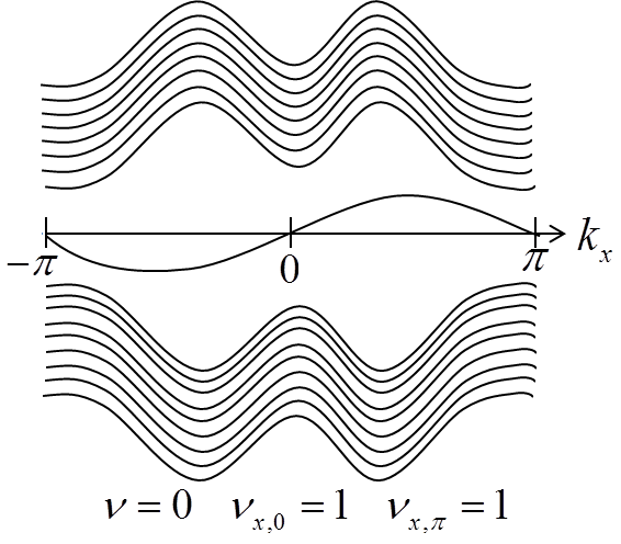 (b)
(b)
 (c)
(c)
It is well-known that the Chern number is equal to the number of edge modes at the edge of the system, weighted by their chirality. These chiral edge modes are robust to any weak perturbations, and do not rely on any particular symmetry. In this sense, a phase with a non-zero Chern number is a strong topological superconducting phase, and the Chern number is a strong topological index. The other indices that characterize the 2D system, and , are only well defined in the presence of translational invariance in the and directions, respectively, and will be referred to as weak topological indices. If at least one of the weak indices is non-zero while the Chern number is zero, the system is in a weak topological phase.
The weak indices can be used to predict certain features of the energy spectrum of gapless edge states that appear on boundaries in specific directions. For example, a straight boundary parallel to the axis that preserves translational invariance in the direction with non-zero () has a zero energy Majorana edge states at (), respectively. Using these properties, it is easy to understand Eq.(6) which relates the weak and strong indices. For example, the two systems whose spectra appear in Fig. 4a and 4c have the same Chern number parity, because there are two edge modes, one at and the other at . Yet, in 4a the edge states have opposite chirality (opposite sign to the slope of the edge state), hence the Chern number is zero. On the other hand, in 4c the edge states have the same chirality. Therefore, the Chern number is . Fig. 4b shows a case where there is only one edge state at , hence the parity of the number of edge states is and the Chern number is .
III Array of quantum wires coupled to a superconducting substrate
In this section, we will discuss a more realistic model that gives rise to the phases described in Sec. II. The first subsection (III.1) will be devoted to a description of the setup, and the second subsection (III.2) to the analysis of the distinct phases arise in the model as a function of the model parameters.
III.1 Setup and model
We envision an array of parallel quantum wires with strong spin-orbit coupling, proximity coupled to a superconductor (Fig. 1). Each wire has a single (spin-unresolved) mode, a large g-factor and strong Rashba spin orbit coupling (this can be achieved, e.g., in InAs or InSb wires[10, 9, 22]). The superconducting substrate induces a proximity gap in the wires. It also allows electrons to tunnel relatively easily from one wire to the next. The system is described by the following Hamiltonian:
| (7) |
Here, , and describe the intra-wire and inter-wire Hamiltonian respectively.
The intra-wire Hamiltonian, is given by
| (8) |
is the Hamiltonian of the th wire, where is the dispersion along the wire ( is chosen to be along the wires, see Fig. 1), is the hopping matrix element along the wire, is the chemical potential, is a Rashba spin-orbit coupling term originating from an electric field perpendicular to the wires (which we define as the direction), and is a Zeeman field along . The Pauli matrices acts in spin space. We have assumed that there is a periodic lattice along the wires, and is the pairing potential induced by the s-wave superconductor. For now, we ignore the orbital effect of the magnetic field; we will consider it in Sec. V.
The inter-wire Hamiltonian is given by:
| (9) |
where is the inter-wire hopping matrix element, is the pairing potential associated with a process where a Cooper pair in the superconductor dissociate into one electron in the th wire and another in the th wire, and is the coefficient of a spin-orbit interaction that originates from inter-wire hopping.
Let us briefly discuss the typical magnitudes of the parameters in Eqs.(8) and, (9). The hopping matrix element is a quarter of the bandwidth of the conduction band in the quantum wires, and is therefore of the order of a few electron-volts. In experimental setups similar to those of Refs. 10, 11, 9, the parameters , , and (the chemical potential measured relative to the bottom of the conduction band) are all of the order of a 0.1-1meV. Therefore, in such setups, is much larger than all the other parameters in the Hamiltonian. One can also imagine suppressing and creating a super-lattice. The super-lattice can be achieved for example by applying a periodically modulated potential along the wires, which would allow the ratio of to the other parameters to be of order unity.
The inter-wire hopping occurs through the superconducting substrate. In order to get a significant inter-wire coupling, the distance between the wires must be at most of order , the coherence length in the s-wave superconductor. The inter-wire spin orbit coupling term depends, mostly on the properties of the material creating the coupling; in the case of nearly touching wires or ribbons this term will depend mostly on the semiconducting material of the wire, such as InAs or InSb. However, when there is a significant distance between the wires, depends mostly on properties of the superconductor; therefore, if the superconductor is made of a light element (such as Al), might be negligible. To get large values of , one would have to use a superconductor made of a heavy element, e.g. Pb. As we will show below, the physics depends crucially on ; if , one can not obtain gaped chiral superconducting phases.
III.2 Phase diagram
We now turn to analyze the phase diagram of the model of Eq.(7). In the limit of decoupled wires, , this is precisely the model studied in Refs. 7 and 8. The phase diagram of each wire consists of two phases, a trivial phase which is realized when , and a topological phase for . The topological phase is characterized by a zero energy Majorana mode at the two ends of each wire[7, 8]. In terms of the two-dimensional topological indices described above, the trivial phase corresponds to , while the non-trivial phase is a weak topological superconducting phase labeled as .
Next, let us consider the effect of inter-wire coupling. We will study the phase diagram as a function of the chemical potential and the Zeeman field for a fixed value of . Imagine starting deep in either the or the phase, and turning on a small inter-wire coupling. Clearly, the inter-wire coupling cannot induce a phase transition as long as it is small compared to the gap. In the vicinity of the phase transition between the and phases, however, the inter-wire coupling can give rise to new phases.

Fig. 5 shows the phase diagram of the model (7) as a function of and for fixed values of , , , and . The phase boundaries were obtained by diagonalizing the Hamiltonian and locating points in the plane were the gap closes. The spectrum of the system is given by
| (10) | |||||
where , and .
The different phases are then identified by using the topological indices of Eqs.(4) and, (5). an explicit calculation of these number is given in Appendix B. Slivers of phases with non-zero Chern numbers appear between the and phases. For example, examining Fig. 5 we note that upon increasing from zero at a fixed negative value of between to (measured in units of ), the gap first closes at and then reopens, and a phase is stabilized. This phase is an anisotropic realization of a chiral superconductor, and has a chiral Majorana edge mode at its boundary. Upon increasing further, the gap at closes and reopens, and the system enters the phase. The points in momentum space where the gap closes can be identified by computing the values of in the Brillouin Zone (See table 1) and locating the point where the sign of changes between the two neighboring phases.
(a)
(b)
As discussed earlier, the experimentally accessible regime in setups similar to those of Refs. 9, 11, 10 is defined by . We highlight the accessible region by a dashed box in Fig. 5. In order to access all the possible phases in Fig. 5, one needs to suppress , for example by applying a periodically modulated potential along the wires, creating a super-lattice.
The spectrum of a system with a finite number of wires in the phase is presented in Fig. 6a, as a function of momentum along the wires. As expected, there are two counter-propagating edge modes within the bulk gap. These modes are localized on the opposite sides of the system.
III.2.1 A phase with a strong index
It is interesting to note that the phase diagram (Fig. 5) contains a phase, with a Chern number and two co-propagating chiral edge modes. This phase appears around for large Zeeman fields (). One can understand qualitatively the emergence of this phase as follows. Focusing in Fig. 5 on the region in which , as the Zeeman field is increased from , the gap closes at and reopens, stabilizing a phase. This phase is characterized by a chiral edge mode, which appears around in a system with a boundary parallel to the axis. Similarly, for the particle-hole conjugated path at , the gap closes and reopens at upon increasing from zero, and one finds a phase with a chiral edge mode around at a boundary along the axis. Near , these two gap closings coincide, and we find a phase that has both a chiral edge modes at and at (see Fig. 6b). We analyze the appearance of this phase in detail in Appendix C.
III.2.2 “Sweet point” with perfectly localized edge states
Interestingly, upon tuning the Zeeman field , there is a special “sweet point” at the center of the phase (as well as in the other chiral phases) in which the chiral states at an edge parallel to the axis are almost entirely localized on the outmost wires. (Notice that the localization lengths of edge states at edges along the and axes are generically different from each other, due to the anisotropy of our system.) At this point, the edge states on the two opposite edges do not mix even in systems with a small number of wires, making it attractive from the point of view of experimental realizability. This point in parameters space is analogous to the special point in the Kitaev’s one-dimensional chain model[5], in which the Majorana end states are localized on the last site. In our two-dimensional setup, we will show how one can access this point by tuning the magnetic field.
We now derive a criterion for realizing the “sweet point”, and give a simple picture for its emergence. First, let us consider a system without coupling between the wires. The Hamiltonian of the th wire Eq.(8) can be written as , where
| (11) |
Here, , and are Pauli matrices acting in Nambu (particle-hole) space.
The strategy in constructing the “sweet point” is as follows. We first tune the parameters of the single wire Hamiltonian Eq.(11) to the critical point at the transition from the trivial to the topological phase. At this point, the low-energy theory is described by two counter-propagating Majorana modes. Turning on the inter-wire coupling induces backscattering between these modes. At the sweet point, the inter-wire coupling takes a special form such that the right moving Majorana mode of one wire couples only to the left moving Majorana mode of the adjacent wire (see Fig. 7). This coupling gaps this pair of modes out, leaving only the two outmost counter-propagating modes gapless. This is similar to the approach of Refs. 23, 24, 25, 26 for constructing quantum Hall phases starting from weakly coupled wires.

Let us demonstrate this by focusing on the single-wire critical point at
| (12) |
in which the gap closes at . We diagonalize the Hamiltonian by a Bugoluibov transformation of the form
| (13) |
where , and the matrix is given by:
| (14) |
Here, . At the critical point, is gapless and disperses linearly, while remains gapped. Expanding near , the Hamiltonian takes the form
| (15) |
where . Inserting Eq.(13) into Eq.(9), and using the explicit form of given in Eq.(14), the inter-wire coupling Hamiltonian projected onto the low-energy () sector becomes
| (16) |
At , the Hamiltonian is identical to Kitaev’s one-dimensional chain model[5] with zero chemical potential. This model simplifies greatly for a special choice of parameters such that . In terms of the physical parameters, this condition is written as
| (17) |
For these parameters, the Hamiltonian is easily diagonalized by introducing Majorana fields
| (18) |
Here, . In terms of these fields, the Hamiltonian takes the form
| (19) |
The resulting phase has two chiral edge modes on the two opposite edges, which are completely localized on the outmost wires, up to corrections of the order of due to virtual excitation to the gapped mode . If the condition in Eq.(17) is not exactly satisfied, the edge states become more spread out in the direction perpendicular to the wires, but remain localized near the boundary as long as the bulk gap does not close.
One can tune into the “sweet point” by setting and such that both Eqs.(12) and (17) are satisfied. The required parameters are and .
We tested the “sweet point” numerically, by diagonalizing the Hamiltonian (7) for a system with a finite number of wires. In Fig. 8, we present the wave functions of the lowest energy states as a function of position perpendicular to the wires. As expected, the wave functions of these states is almost localized on the outmost wires.
III.2.3 In-plane Zeeman magnetic field
Applying an in-plane magnetic (Zeeman) field provides an additional experimentally accessible knob to tune the system between different phases. We now consider its effect on the phase diagram. Note that in our system, a perpendicular magnetic field is essential in order to realize the strong topological phase (this is different from the case considered in Ref. 14, due to the different form of the spin-orbit coupling). The in-plane magnetic field generally destroys the topological phases, leading to a gapless phase instead.
In the presence of an in-plane Zeeman field applied parallel to the wires, we should add the term to Eq.(8). Then, the spectrum is given by
| (20) |
where . The condition for a closer of the gap is:
| (21) |
Fig. 9 shows the phase diagram as a function of and , fixing . The line corresponds to a line of fixed of the phase diagram shown in Fig. 5. Upon raising , a gapless (metallic) region is formed. The gap closes because of the destruction of the proximity effect by the in-plane field, due to the Zeeman shift of the normal state energy at relative to . The effect of an in-plane field perpendicular to the wires () is qualitatively similar, but the “bubbles” of the phase do not appear, and are replaced by gapless regions. (Notice that the response for a Zeeman field in the and directions is different because of the anisotropy of our system.)
One can also show that the “sweet point” within the strong topological phases survives in the presence of an in-plane field. The sweet point condition is given by Eqs.(17) and (21).

IV The orbital effect of the magnetic field in a 2D p-wave superconductor
So far, we have neglected the orbital effect of the magnetic field, treating only the Zeeman effect. This assumption is justified in the limit of large g-factor, . In this section, we will consider the orbital effects of the magnetic field.
We begin by discussing the condition for the appearance of vortices in our system. We assume that the s-wave superconductor is a narrow strip, whose width is small compared to its length and to the bulk penetration length. Under these conditions, the critical field for creating a single vortex in the superconductor is[27] , where . This gives .
To get a feeling for the value of this critical field in realistic setups, let us consider a system with wires made of InAs, similar to those of Ref. 10. We assume that the distance between the wires is of order (ensuring a reasonable inter-wire coupling). If we take (as in Pb) and , we get and the critical magnetic field for creating a single vortex is . In order to be in the topological phase the Zeeman field must satisfy (where is the induced superconducting gap in the wire). In InAs, and can be of the order of [10]. This gives that the required magnetic field to be in the topological phase is , and thus vortices are present in the strip. As we decrease the size of the system, the critical field increases. For a system with and , for example, the critical field is , and one can realize a vortex-free topological phase.
Below, we discuss features of the quasi-particle spectrum in the presence of an orbital field that can be used as a signature of topological phase in the system.
IV.1 Majorana zero modes in vortex cores
The chiral phase is characterized by the presence of a Majorana zero mode at each vortex core[4]. For an applied field slightly above , the ground state contains vortices along the strip, with a Majorana zero mode at each core. In addition, when the number of vortices is odd, the chiral Majorana mode on the edge has a mid-gap state. In general, the Majorana states in the vortex core can leak into the edge mode. However, if we choose parameters such that the system is near the sweet point described above, such that the effective coherence length transverse to the wires is essentially one inter-wire spacing, the mixing between the vortex core states and the chiral edge modes can be made negligibly small (assuming that the wires are sufficiently long), as can be seen in Fig. 11. One can show that the sweet point condition, Eq.(17), remains unmodified when projecting to the lower energy bands to leading order in the orbital magnetic field (see Appendix E).
IV.2 Doppler shifted chiral edge states
In addition to inducing vortices, the orbital field induces circulating orbital currents in the sample. These orbital currents modify the low-energy density of states (DOS) due to a “Doppler shift” of the quasi-particles at the edge. In a chiral superconductor, the Doppler shift either enhances or suppresses the DOS at the edge, depending on whether the orbital supercurrent is parallel or anti-parallel to the propagation direction of the chiral edge state[28]. Using the London gauge near the edge, such that (where is the phase of the order parameter), the external orbital current is proportional to the vector potential . Consider a system defined on the half-plane , with an edge at . To linear order in and , The low-energy quasi-particle spectrum is given by
| (22) |
The velocity and the coefficient can be calculated perturbatively in and . In the model described in Sec. III, the perturbative calculation gives and . See Appendix D for an explicit derivation of this result. Since the local DOS is proportional to the inverse of , Eq.(22) shows that the zero-energy DOS depends linearly on [28]. Fig. 10a shows how the slope of the chiral edge state changes when the orbital magnetic field is not negligible. Similarly, one can calculate the spectrum of the edge mode at an edge parallel to . For such an edge, and .
Surprisingly, the linear dependence of the local DOS at the edge on the supercurrent is not limited to the strong (chiral) topological phases, but exists also in the weak phases. E.g., consider a system in the phase with a straight edge parallel to . There are low-energy edge modes near and , whose dispersions have opposite slopes. The dispersion of the edge mode near is given by , to linear order in . Therefore, if we apply a supercurrent near the edge such that the slope of the edge mode at increases in magnitude, the slope of the mode at increases as well, and the total DOS at the edge decreases linearly with the current, as can be seen in Fig. 10b.
In general, a linear dependence of the DOS on the supercurrent is possible if time-reversal symmetry is broken. In our system, time-reversal is broken by the external magnetic field, which is present both in the weak and the strong topological phases. In the weak phases, the edge modes do not carry current; nevertheless, a supercurrent couples to the edge modes through the phase of the condensate.
(a)
(b)
In the presence of vortices, the orbital effect leads to an interesting variation of the low-energy local DOS at the edge. Each vortex produces circulating supercurrent. Therefore, the superfluid velocity at the edge varies as a function of position; it is either enhanced or suppressed in regions of the edge which are close to a vortex core, depending on the chirality of the vortex relative to that of the superconductor. (In our system, the relative chirality of the vortices and the superconductor depends on the signs of the spin-orbit coupling terms and , and is not easy to control externally.) Therefore, according to Eq.(22), the local DOS at the edge shows either a dip or a peak in the vicinity of a vortex in the bulk.
(a) (b)
(b)
(c) (d)
(d)
We tested this effect numerically for a finite system with a single vortex. Fig. 11 shows the probability distribution of the two lowest energy states in the system. We used two sets of parameters, one in which the vortex has the same chirality, as shown in Fig. 11a, and the other in which it has opposite chirality Fig. 11b, relative to the superconductor. The low-energy states are superpositions of a localized zero mode at the vortex core, and a propagating mode localized on the edge. The variations of the probability distribution of the edge mode are proportional to the variations of the local DOS on the edge. As expected, the local DOS is either enhanced (second row, Fig. 11c and Fig. 11d) or suppressed (first row, Fig. 11a and Fig. 11b) in the region of the edges close to the vortex. The vortex is incorporated in our model by multiplying the order parameter by a spatially dependent phase factor such that , where . The vector potential was taken to be .11 1 We expect the splitting between the two eigenenergies closest to zero to scale as , where is the size of the system in the direction and is the corresponding coherence length. (We assume that .) The corresponding eigenstates are linear combinations of the localized Majorana state at the vortex core and a Majorana mode bound to the edge. The next lowest energy scales as , due to the finite size in the direction.
The Doppler shift effect is a signature of all the topological phases. It can be observed by measuring the tunneling current into the edge in the presence of a supercurrent along the wire direction. Since, in the London gauge, , According to Eq.(22), the low-energy DOS depends linearly on the current.
V Distinguishing between the different phases experimentally
In this section, we discuss ways to distinguish experimentally between the different phases shown in Fig. 5. The results are summarized in Table 1. These phases can be divided into two groups: the strong topological phases characterized by , and the weak topological phases characterized by . Each of the phases is characterized by the appearance of Majorana modes at specific momenta along the edge. The topological phases can be determined by measuring the tunneling conductance from a metallic lead into the edges.
| Edge states (non-chiral Majorana modes) | Tunneling DOS from a local tip | ||||||
|
Trivial |
None | 0 | 0 | ||||
| weak phases | Along the edge | 0 | Finite | ||||
| Along the edge | Finite | 0 | |||||
| Along the edges and | Finite | Finite | |||||
|
Chiral Edge states along the edges and
, located near and
, respectively |
Tunneling DOS from a wire | ||||||
| Strong phases | , | Finite | Finite | 0 | 0 | ||
| , | Finite | 0 | 0 | Finite | |||
| , | 0 | Finite | Finite | 0 | |||
| , | 0 | 0 | Finite | Finite | |||
| * | Two edge modes at , | ||||||
| and , | Finite | Finite | Finite | Finite | |||
In the upper table, the first line is the trivial phase. Lines 2-4 describe the weak topological phases, which can be distinguished by measuring the local tunneling density of states at low energy on the edges perpendicular and parallel to the wires.
The lower table lists the strong topological phases. These phases cannot be distinguished from each other using a local tunneling probe, since they all have low-energy chiral modes on all edges. The phases differ in the position of the edge states in momentum space (see Fig. 4). Hence, they can be distinguished in a tunneling experiment from an extended wire, such that the momentum along the edge is conserved in the tunneling process (as in the experiments of Ref. 29). The momentum probed in the tunneling experiment can be tuned by varying the flux between the wire and the edge of the system[29].
(*) The and phases have identical weak indices. Therefore, they cannot be distinguished by tunneling experiments. In order to resolve them, one would need additional experiments (e.g., a measurement of the thermal Hall conductance[4]).
The strong phases are characterized by the presence of chiral edge states along any edge, regardless of its direction. The weak phases, on the other hand, may have low-energy edge states on a boundary along , , or both, depending on the values of the weak indices. The presence of an edge state near a given momentum can be determined from the indices [defined above Eq. (4)]. For example, a low-energy state appears along the edge parallel to near momentum if , and so forth.
Scanning tunneling spectroscopy (STS) experiments, in which electrons tunnel from a point-like tip into the sample, will detect a finite tunneling conductance at low energy on all boundaries in the strong phase. Finding a finite conductance on a boundary along but zero conductance on a boundary along (or vise versa) is a signature of a weak phase. In all cases, the bulk of the system is fully gapped.
Phases with different weak indices can be distinguished in momentum-resolved tunneling experiments. One can imagine tunneling from an extended wire into the boundary of the system, so that the momentum along the boundary is approximately conserved. A perpendicular magnetic field can be used to control the momentum transfer in the tunneling process[29]. This way, one can isolate the contributions to the tunneling density of states from the vicinity of and along the boundary.
Table 1 summarizes the different possible phases and their signatures in STS experiments, as well as momentum-resolved tunneling experiments at momentum or along the boundary. By combining these experiments, many of the phases can be distinguished from each other. However, the , and phases have identical weak indices (see Table 1), hence tunneling experiments can not distinguish between them. In order to resolve them, one would need additional experiments (e.g. a measurement of the thermal Hall conductance[4]). Notice, however, that neither the 0:11 nor the phases occur naturally in our coupled-wire setup (see dashed region in Fig. 5). As discussed in subsection III.2.1 the phase can be realized in a super-lattice structure, and appendix A describes a possible realization of the phase.
VI Conclusions
In this work, we studied an array of weakly coupled superconducting wires with spin orbit coupling. This system can be used to realize a rich variety of two-dimensional topological phases, either of the “weak” or “strong” kind. One can tune between different phases using experimentally accessible parameters, such as the chemical potential and the magnetic field. The strong phases are anisotropic analogous to the chiral phase, and have chiral (Majorana) edge modes at their boundaries.
In particular, there is a choice of parameters such that the chiral edge states are almost completely localized on the two outmost wires. At this “sweet point”, the edge states on the two opposite edges do not mix even in a system with few wires. Similarly, at this point in parameters space, the Majorana zero mode at a vortex core is tightly localized in the direction perpendicular to the wires, and resides only on one or two wires.
Each one of the topological phases has a unique signature in its edge spectrum. The different phases can be distinguished in tunneling experiments into the edge. Moreover, density of states of the Majorana edge modes is predicted to vary linearly with an applied supercurrent in the wires.
Acknowledgements.
We would like to acknowledge discussions with Y. E. Kraus, A. Keselman, A. Haim, Y. Schattner, and Y. Werman. E. B. was supported by the Israel Science Foundation, by a Marie Curie CIG grant, by the Minerva foundation, by a German-Israeli Foundation (GIF) grant, and by the Robert Rees Fund. Y.O. was supported by an Israel Science Foundation grant, by the ERC advanced grant, by the Minerva foundation, by the TAMU-WIS grant, and by a DFG grant.Appendix A The topological phase 0:11
The topological phase does not appear in the physical system of coupled wires, or in the simplified model described in Sec. II. One can imagine a different setup that realizes this phase, such as the one presented in Fig. 12. Consider two layers of weakly coupled parallel wires, rotated by relative to each other. Initially, suppose that there is no coupling between the two layers. One of the layers is in the phase (i.e., adiabatically connected to a phase of decoupled 1D topological superconductors oriented along the direction), and the other is in the phase. If we turn on a weak coupling between the two layers, we get a single two-dimensional system whose indices are the sums of the indices of the two constituents (modulo 2). The entire system is therefore in the phase.

The phase is characterized by having non-chiral Majorana edge modes at low energy on edges along the or directions. More generally, on an edge directed along an angle such that (where are integers), there is a low energy Majorana mode if is odd. This can be seen from fact that such an edge preserves translational invariance along . If we turn off the coupling between all the wires (both within each layer and between the layers), every unit cell of the edge contains Majorana zero modes. Upon turning on inter-wire coupling, we get an edge mode that crosses zero energy at momenta and parallel to the edge if the number of Majorana zero modes per primitive unit cell is odd. Otherwise, we can pair the Majorana zero modes within each unit cell and gap them out.
It is interesting to consider the case of an edge such that is irrational. In this case, the edge breaks translational symmetry, so we cannot define the number of Majorana modes in a unit cell in the decoupled limit. On physical grounds, we expect to get a gapless mode in this case, since we can approximate by arbitrarily well, with odd.
Appendix B Computation of the topological invariants in an array of coupled quantum wires
The Hamiltonian Eq.(7) in momentum space is given by , where , and
| (23) |
Here, . The Hamiltonian has particle-hole symmetry, , where . According to Eqs. (4), the topological indices depend only on the Hamiltonian at the high symmetry points . At these points, it is convenient to transform to the Majorana basis: , where ( are Majorana operators) and
| (24) |
In this basis, the Hamiltonians at the high symmetry points are given by
| (25) |
The Pfaffians of can be computed using the relation
In our case, , , , , and . This gives . From this, the indices can be computed using Eq.(4). It also enables us to produce the phase diagram as depicted in Fig. 5 up to the parity of the Chern number using Eq.(6). We have calculated the Chern number numerically and verified these conclusions. The calculation was done with periodic boundary conditions in both directions, using the formula[3]:
| (26) |
where is a projection operator on the negative energy bands, defined as . Substituting into Eq.(26), we arrive at Eq.(5). In Appendix C we give an analytical explanation for the existence of the strong index in the phase diagram.
Appendix C Explanation for the existence of the strong index in the phase diagram
In order to understand the appearance of a phase with a strong index in the model described in Sec. III, we analyze the changes in the Chern number along a trajectory in the parameter space . Along the line and , the gap closes at [see Eq.(10)]. At each of these points in the parameter space, the closure of the gap occurs simultaneously at two points in the Brillouin zone. E.g., at , the gap closes at and , whereas at , the gap closes at and .
Near these points, the low-energy part of the spectrum is linear (Dirac-like). Tuning away from , Dirac mass terms appear. The vicinity of each Dirac point in the Brillouin zone contributes to the total Chern number, where is the Dirac mass. Thus, a sign change in the mass term corresponds to a change in the total Chern number by . Below, we derive the form of the massive Dirac Hamiltonians at the vicinity of . We show that the Chern number changes by as is swept through .
First, we project the Hamiltonian in Eq. (23) to the two bands closest to zero energy. At the critical point , the zero-energy eigenstates are , . Here , , and . The effective Hamiltonians in the vicinity of and near the critical point are given by
Here, .
At sufficiently large , the strong index is . Crossing through , the contributions to the Chern number from the vicinity of is given by
| (27) |
Therefore, the change in the Chern number from to is . In the same way, tuning through from above changes the Chern number by .
Appendix D Quasi-particle spectrum in the presence of orbital magnetic field
In this appendix, we will show that the density of states of the edge modes in the presence of an orbital magnetic field (or a supercurrent parallel to the edge) is linear in the vector potential. We consider a BdG Hamiltonian of the form , using the Nambu notation: , and
| (28) |
Here, is the normal (non-superconducting) Hamiltonian, and is the pairing matrix. We note that the particle-hole symmetry is expressed in this basis as follows: . This implies . Hence, the spectrum should satisfy
| (29) |
.
We now consider a semi-infinite system with periodic boundary conditions in the direction and half-infinite in the direction. The equations for the eigenstates acquire the form: , where is a matrix whose indices are the wire labels, and runs over all the eigenstates.
Let us assume that there is a single Majorana edge mode at and that . Expanding the edge mode energy, , near and , we get
Particle-hole symmetry [see Eq.(29)] requires that and . We denote , . The coefficients and can be calculated using:
| (30) |
| (31) |
Substituting , we can arrive to the following formula:
For the model described in Sec. III, and has the following form near :
In the sweet point, discussed in III.2.2, the edge state at is completely localized on the outmost wire. In the limit , we can evaluate Eqs.(30), (31), and (32) perturbatively in and . To zeroth order, we can replace the wave-functions () with the eigenstates of the decoupled wires (). Using the explicit form of the single wire eigenstates, , and their particle-hole partners [given in Eqs.(14) and (13)], we get
| (33) |
Appendix E The effect of the orbital field on the “sweet point”
Here, we demonstrate that the ”sweet point” condition [Eq.(17)] is not modified in the presence of a small orbital magnetic field.
Let us consider a system with a uniform orbital field. The single-wire part of the Hamiltonian is given by:
| (34) |
Here, is the flux per unit cell, and . We have used the Landau gauge, such that .
Applying the same procedure as in Sec. III, the Hamiltonian matrix at is given by:
| (35) |
For a sufficiently small orbital field such that 22 2 Taking where is the a typical spin orbit coupling length and is a typical spin orbit energy. Since , the factor in the inequality condition cancels and we find the condition . For , the requirement is . In the experiments [10, 9] this condition is only marginally satisfied. (where is the width of the system), we can treat the orbital field perturbatively. To zeroth order in , the single wire Hamiltonian at the critical point [Eq.(12)] is diagonalized by a Bogoliubov transformation specified in Eq.(14). In terms of the eigenstates and , the vector potential term is
| (36) |
Here, . Upon projecting the Hamiltonian onto the low-energy () sector, this term is zero as it couples and . Therefore, to first order in , the inter-wire Hamiltonian projected to the low-energy subspace retains the form of Eq. (16). I.e., to first order in , the “sweet point” condition [Eq.(17)] in unaffected.
References
- [1] M. Z. Hasan and C. L. Kane, Reviews of Modern Physics 82, 3045 (2010).
- [2] X.-L. Qi and S.-C. Zhang, Reviews of Modern Physics 83, 1057 (2011).
- [3] B. A. Bernevig, Topological insulators and topological superconductors (Princeton University Press, 2013).
- [4] N. Read and D. Green, Physical Review B 61, 10267 (2000).
- [5] A. Y. Kitaev, Physics-Uspekhi 44, 131 (2001).
- [6] A. Kitaev, Annals of Physics 303, 2 (2003).
- [7] R. M. Lutchyn, J. D. Sau, and S. D. Sarma, Physical review letters 105, 077001 (2010).
- [8] Y. Oreg, G. Refael, and F. von Oppen, Physical review letters 105, 177002 (2010).
- [9] V. Mourik, K. Zuo, S. Frolov, S. Plissard, E. Bakkers, and L. Kouwenhoven, Science 336, 1003 (2012).
- [10] A. Das, Y. Ronen, Y. Most, Y. Oreg, M. Heiblum, and H. Shtrikman, Nature Physics 8, 887 (2012).
- [11] M. Deng, C. Yu, G. Huang, M. Larsson, P. Caroff, and H. Xu, Nano letters 12, 6414 (2012).
- [12] H. Churchill, V. Fatemi, K. Grove-Rasmussen, M. Deng, P. Caroff, H. Xu, and C. Marcus, Physical Review B 87, 241401 (2013).
- [13] L. P. Rokhinson, X. Liu, and J. K. Furdyna, Nature Physics 8, 795 (2012).
- [14] J. Alicea, Physical Review B 81, 125318 (2010).
- [15] J. D. Sau, R. M. Lutchyn, S. Tewari, and S. D. Sarma, Physical review letters 104, 040502 (2010).
- [16] L. Fu and C. L. Kane, Physical review letters 100, 096407 (2008).
- [17] D. Asahi and N. Nagaosa, Physical Review B 86, 100504 (2012).
- [18] A. Kitaev, in AIP Conference Proceedings, Vol. 1134 (2009) p. 22.
- [19] A. P. Schnyder, S. Ryu, A. Furusaki, and A. W. Ludwig, Physical Review B 78, 195125 (2008).
- [20] L. Fu and C. L. Kane, Physical Review B 76, 045302 (2007).
- [21] D. J. Thouless, M. Kohmoto, M. P. Nightingale, and M. den Nijs, Physical Review Letters 49, 405 (1982).
- [22] R. M. Lutchyn, T. D. Stanescu, and S. D. Sarma, Physical Review Letters 106, 127001 (2011).
- [23] C. Kane, R. Mukhopadhyay, and T. Lubensky, Physical review letters 88, 036401 (2002).
- [24] J. C. Teo and C. Kane, arXiv preprint arXiv:1111.2617 (2011).
- [25] S. Sondhi and K. Yang, Physical Review B 63, 054430 (2001).
- [26] R. S. Mong, D. J. Clarke, J. Alicea, N. H. Lindner, P. Fendley, C. Nayak, Y. Oreg, A. Stern, E. Berg, K. Shtengel, et al., arXiv preprint arXiv:1307.4403 (2013).
- [27] G. Stan, S. B. Field, and J. M. Martinis, Physical review letters 92, 097003 (2004).
- [28] T. Yokoyama, C. Iniotakis, Y. Tanaka, and M. Sigrist, Physical review letters 100, 177002 (2008).
- [29] O. M. Auslaender, H. Steinberg, A. Yacoby, Y. Tserkovnyak, B. I. Halperin, R. de Picciotto, K. W. Baldwin, L. N. Pfeiffer, and K. W. West, Solid state communications 131, 657 (2004).