Comparison of the gradient flow with cooling in pure gauge theory
Abstract
The gradient (Wilson) flow has been introduced recently in order to provide a solid theoretical framework for the smoothing of ultraviolet noise in lattice gauge configurations. It is interesting to ask how it compares with other, more heuristic and numerically cheaper smoothing techniques, such as standard cooling. In this study we perform such a comparison, focusing on observables related to topology. We show that, already for moderately small lattice spacings, standard cooling and the gradient flow lead to equivalent results, both for average quantities and configuration by configuration.
pacs
11.15.Ha, 11.15.Kc, 12.38.Aw.I Introduction
At present, the lattice formulation represents the best available tool for a gauge-invariant regularization [1] and a systematic non-perturbative numerical study of strong interactions, and, more generally, of gauge theories. Like for any regularized theory, one has to deal with unphysical fluctuations at the scale of the ultraviolet (UV) cutoff (which is set by the lattice spacing in the case of lattice gauge theories), which must be properly treated. Over the years, various techniques have been developed in this sense. Where possible, proper prescriptions can be assigned for a perturbative or non-perturbative renormalization of physical quantities. Another widely used technique is instead to apply some kind of smoothing procedure, in order to dampen the fluctuations at the UV scale, while hopefully leaving the physical content unchanged.
Typical examples of observables requiring renormalization are the topological charge (winding number) and, more generally, the observables related to topology, like the topological susceptibility. Contrary to its continuum counterpart, the lattice gluonic definition of the topological charge is affected by UV fluctuations: it gets multiplicatively renormalized [2] and does not take integer values. Further additive renormalizations, related to contact terms, appear when defining the topological susceptibility [3].
Apart from switching to a fermionic definition of topology, via the index theorem, various strategies have been developed to successfully deal with such renormalizations, going from a direct computation and subtraction of them [4, 5, 6, 7, 8, 9, 10] to the application of smoothing methods to dampen the UV fluctuations and recover an almost integer valued observable. In this respect, cooling techniques [11], which proceed through a local minimization of the gluonic action, are particularly well suited, since the topological content of gauge configurations becomes quasi-stable against minimization as one approaches the continuum limit, i.e. as one recovers a proper definition of the gauge field topology.
In this context, the recent introduction of the gradient flow (also known as Wilson flow when used in connection with the Wilson action) represents an important advance [12, 13]. The main difference with respect to previously used smoothers is that in this case the elimination of UV fluctuations is governed by a differential equation, thus achieving a better analytical control of the smoothing procedure.
An interesting and due question regards how the gradient flow compares with other standard smoothing techniques. The present study is a step in the direction of clarifying this issue. In particular we will compare standard cooling and the gradient flow, for the determination of topological observables, in the lattice gauge theories discretized with the Wilson action.
Such a question is of general interest, since standard smoothing techniques have been widely used in the literature. But it is also of great practical interest. Indeed, as we will clarify later, the application of the gradient flow is much more computationally demanding than standard cooling. It is therefore compelling to understand what the effective differences are between the two methods, depending on the chosen observable.
The paper is organized as follows. In Section II we provide a brief description of the gradient flow and of standard cooling and then compare them in the limit of smooth fields. In Section III we first discuss the definition of a general setting for the comparison of the two methods; then we present our numerical results for topological quantities. Finally, in Section IV, we discuss our results and draw our conclusions.
II Cooling and the gradient flow
In this section, for the benefit of the reader, we recall the definitions of the gradient flow and of the cooling procedure, and present the details of our implementation. We will limit ourselves to the case of the Wilson action for pure gauge theories [1], which is the one used in our simulations, but the generalization to different discretizations does not present significant difficulties.
The Wilson action is written in terms of the product of the link variables along an elementary face (plaquette) of the lattice, , in the form
| (1) |
where is the number of colors. It is convenient to introduce the staples as the (in general non unitary) matrices , defined by
| (2) | ||||
the part of the action involving a given link variable is then simply written as . To avoid confusion, in the following expressions we will not make use of the implicit summation over repeated indices.
II.1 Gradient flow
The gradient flow is defined (see [12, 13]) by the solution of the evolution equations
| (3) | ||||
where the link derivatives are defined by
| (4) | ||||
In this expression are the (hermitian) 11 1 We would like to warn the reader that such a notation is different from the one adopted in the literature where the gradient flow has been originally discussed [12, 13]. We follow here the standard convention in which the generators of are taken to be hermitian, e.g., for , where are the Gell-Mann matrices. generators of the algebra, with the normalization , and
| (5) |
If we introduce the notation we have
| (6) |
and is given by
| (7) | ||||
In practice, the gradient flow moves the gauge configuration along the steepest descent direction in the configuration space, i.e. along the gradient of the action (hence the name of gradient flow); in particular, the chosen sign in the evolution equations leads to a minimization of the action. Indeed, from the definition Eq. (3) and the previous expressions it is simple to show that
| (8) |
Thus is a monotonically decreasing function of the flow time and the “evolved” variables can be used as the smoothed version of the original link variables . From the explicit expression, Eq. (7), we can also see that the gradient flow is just the flow generated by the infinitesimal version of the isotropic stout smearing introduced in Ref. [14]. It is important to stress at this point that quantity , defined here and used in the following, is the flow time in dimensionless units.
The integration of the flow in Eq. (3) can be performed by using standard methods for ordinary differential equations; in particular, we adopted the third order Runge-Kutta scheme described in appendix C of Ref. [13]. We have chosen an elementary integration step , and verified that the integration error induced by this choice does not significantly affect our results 22 2 In particular, results obtained on a subsample of configurations by using a different integration step, , are indistinguishable from those obtained at ..
II.2 Cooling
Also in the case of cooling, the idea is that of evolving the gauge configuration so as to minimize the gauge action: in fact, cooling has been one of the first procedures introduced to get rid of UV artifacts by smoothing gauge configurations [11]. However, while the gradient flow is defined by an evolution equation, the cooling method proceeds by discrete steps: in each step the action is minimized with respect to a subset of configuration variables (e.g., a single link or even a link subgroup), and then the procedure is performed iteratively over all variables, in order to achieve a global movement of the configuration towards the minimum of the gauge action.
Many variants of cooling have been devised, in which the discrete steps are made more or less smooth [15, 16]. Here we will consider the simplest, original version, also known as standard cooling:
- •
An elementary step of the algorithm consists in replacing a given link variable by the group element which locally minimizes the action, while all other link variables are kept fixed, i.e. by the matrix which maximizes
In the particular case of the gauge theory, the maximization step can be performed analytically, with the result
For the maximization is performed by using a Cabibbo-Marinari like algorithm ([18]), i.e. by iterating the maximization over a covering set of subgroups.
- •
The procedure is then repeated iteratively by visiting link variables on all sites and along all directions of the lattice. In our implementation we will first sweep lattice sites, following the standard lexicographic order, and then link directions, starting with and . Both the starting link and the visiting order can be changed at will, leading to slightly different cooling variants.
- •
A complete sweep of the lattice is what is usually called a cooling step. A cooling step can be iterated times, thus generating a (discrete) flow in the space of gauge configurations.
It is important to stress once more that, contrary to other smoothing procedures such as smearing, a cooling sweep proceeds iteratively, i.e. at each elementary step the cooled link is substituted in the configuration before computing the staple needed to cool the next link. If staples were all computed before starting the cooling sweep, the decrease of the action would not be guaranteed anymore, and instabilities would appear, similar to those happening in the repeated application of smearing when the smearing parameter is too large (see, e.g., Ref. [17]). This iterative nature of cooling will be important when discussing the speed at which cooling proceeds, as compared with the gradient flow.
It is interesting to notice that there is one variant of cooling which resembles the gradient flow more closely, namely the controlled cooling introduced in Ref. [15]. In that case, the elementary step of cooling consists in minimizing the action under the constraint
| (9) |
where and are, respectively, the old and the new link variables. Also in this case the configuration proceeds towards a minimum, but with the constraint that at each elementary step the new link variable does not differ much from the old variable, depending on the value of the controlling parameter . For small enough , the cooling step effectively becomes an infinitesimal movement along the steepest descent direction, i.e. it becomes a possible integrator of the gradient flow. Indeed, the authors of Ref. [15] verified that, for small enough , the order in which the links are cooled becomes immaterial.
| 5.95 | 4.898(12) | 0.1021(25) |
|---|---|---|
| 6.07 | 6.033(17) | 0.08288(23) |
| 6.2 | 7.380(26) | 0.06775(24) |
II.3 Perturbative relation between the two smoothing procedures
As we have already stressed, both cooling and the gradient flow evolve the gauge configuration towards a minimum of the gauge action. In a perturbative approximation, in which all link variables are very close to the identity element of the gauge group, the connection between the two procedures can be investigated in more detail, and a relation can be found between the speed at which the two evolutions proceed. This relation will be compared with the numerical results in Section III.
Let us assume, therefore, that for each link variable, so that the staple takes the simple form , where both and are infinitesimal quantities. In this approximation, one has
and Eq. (7) becomes
| (10) |
As a consequence, the evolution equation of the gradient flow can be approximated as follows:
| (11) |
On the other hand, cooling acts so as to substitute with the projection of over the gauge group. In the perturbative approximation, this projection is simply , so that the elementary cooling step corresponds to the substitution
| (12) |
A naive comparison of Eqs. (11) and (12) would lead to the conclusion that the instantaneous speed at which links evolve in the gradient flow is such that a whole cooling step would be covered in a step of gradient flow evolution, i.e. that the approximate relation should hold between the gradient flow time and the number of cooling steps. The factor 6 comes, given the normalization chosen for the gradient, from the number of staples around a given link, i.e. it is equal to , where is the number of space-time dimensions.
However, such a conclusion is wrong by a factor , as is clear from the following argument. The staple appearing in the gradient flow is constructed with gauge links all computed at the same flow time . On the contrary, in the case of cooling, due to the iterative nature of the process, some of the links used to construct the staple have already undergone the cooling step under consideration, and this results in an increase in the speed of cooling. For a regular visiting order of the lattice links during the sweep, one has that, on average, that half of the neighboring links have already been cooled one more time: that results in a speed increase for cooling by a factor 2 with respect to the naive expectation, as one can evince from the simple diffusive model discussed in Appendix A.
Therefore, the predicted perturbative relation is actually . Such a relation is expected to depend on the dimensionality of the system (and on the normalization of the gradient, i.e. on the fact that we actually take the gradient of ), but not on the number of colors, at least in the limit of smooth fields.
II.4 Smoothing and the continuum limit
Let us now discuss how smoothing has to be tuned as the continuum limit is approached. An important point is that this tuning is independent of the particular kind of smoothing, be it cooling, the gradient flow or something else, once a precise correspondence has been found between the different techniques, which is valid lattice spacing by lattice spacing.
Smoothing is, in general, an arbitrary modification of the theory in the UV, up to some length scale , with the only requirement that it dampens the quantum fluctuations on length scales smaller than . While smoothing changes the theory up to , we have to ensure that this does not affect our continuum results, i.e. that physics does not depend on the choice of . If we are studying an observable which is naturally defined for large distances only, an obvious example being the effective mass extracted from the expectation value of a correlator, then it is natural to keep fixed in physical units: to avoid systematical dependences on , it will be sufficient to use correlators defined at distances .
This possibility is particularly appealing in the gradient flow setup, since it can be shown that composite operators defined at fixed physical flow time renormalize in a simple way (see Ref. [19]). In particular, for the case of the gradient flow one has
| (13) |
where is the flow time in physical units (see Ref. [13]), being the lattice spacing. This procedure can now be simply translated in terms of cooling. Indeed from the argument of the previous section (i.e. ), which will be accurately verified against numerical results in the following sections, we expect for cooling the analogous relation
| (14) |
i.e. the number of cooling steps has to be scaled proportionally to in order to keep fixed. Actually this is not a completely new result, since it is already well known that cooling acts like a diffusive process.
The situation can be less trivial for observables which are not related to large distance correlators, but are instead an integral over all distances of some two point function, like a susceptibility. In this case it is not guaranteed apriori that keeping fixed will not affect the continuum limit, and one must look for the existence of a proper “safe scaling window” for (see Ref. [20] for a discussion regarding the gradient flow).
An example is the topological susceptibility, which is the integral over all distances of the two point correlator of the topological charge density. In this case one can follow different strategies to look for the safe scaling window. A known procedure [21] is to look for a plateau in terms of at every fixed lattice spacing, and then perform the continuum extrapolation of the plateau values. The existence of the plateau ensures that is small enough not to affect the physical result and that, on the other hand, the smoothing is effective in removing additive and multiplicative renormalizations.
Alternatively, one could perform the continuum limit of results obtained at fixed , and then look for a safe plateau, in terms of , in the continuum extrapolated values. It is not the purpose of this study to perform an accurate check of the consistency of these two strategies. What we will show, instead, is that two perfectly equivalent definitions of exist at every fixed lattice spacing, Eq. (13) and Eq. (14), defined by either cooling or the gradient flow, in terms of which one can perform the preferred continuum extrapolation.
III Numerical results
Most of the simulations have been performed on a lattice at the bare coupling values , corresponding to the lattice spacings reported in Table 1 and to physical lattice sizes ranging from to . Here We do not have the aim to keep finite size effects well under control, since our purpose is simply the check how cooling and the gradient flow compare to each other, on the same configuration sample, in the smoothing of fluctuations at the UV scale. However, a comparison with some simulations performed on larger lattices shows that such effects are not large and do not significantly affect our conclusions.
For each value of the bare coupling we have generated configurations, each one separated from the next by Monte Carlo steps, a single step consisting of a full lattice update with heatbath ([23, 24]) and overrelaxation sweeps ([25]). On these configurations, we have evaluated the topological charge after smoothing, by using both cooling (we have reached a maximum of cooling steps, with measurements taken after each step) and the gradient flow (reaching a maximum flow time , with measurements performed every ). The expression used for the discretization of the topological charge density is
| (15) |
where for positive indices, while for the negative directions the relation and the complete antisymmetry are used.
III.1 Setting a common scale

The purpose of the present study is to compare how the (continuous) gradient flow and the discrete flow generated by cooling compare to each other. It is clear that, in order to do that, we need to set a common scale, i.e. to fix apriori what is the flow time to be compared with cooling steps. The simplest way to proceed is to set such a common scale by using some standard observable, and the most natural observable is given by the quantity whose minimization defines both flows, that is by the action itself. This is also the strategy adopted in the past to compare different versions of cooling [26].
In Fig. 1 we report the average plaquette (action density) values as a function of (for cooling) and of (for the gradient flow case). Such functions permit to obtain the desired correspondence: for each given value of the inverse bare gauge coupling , we define as the value of the gradient time that changes the average action by the same amount as cooling steps.
A plot of the functions , obtained for the different explored values of , is shown in Fig. 2: the agreement among the different lattice spacings is striking and demonstrates that the correspondence between cooling and the gradient flow has a perfectly well-defined continuum limit. The continuous line corresponds to the function . It is clear that this function is a good approximation of for all the lattice spacings used, and becomes better and better as increases: the agreement is at the level of 1% for and of 0.1% (i.e. already within the precision of our determination) for . In the following, for simplicity, we will just use the approximation , which is equivalent to saying that one unit of gradient flow time corresponds to three cooling steps; corrections to this assumptions prove to be completely irrelevant to the following analysis. Preliminary results show that the relation holds true also for the gauge group , thus supporting the perturbative argument of the previous section.

III.2 Determination of the topological background
The lattice topological charge is defined as the sum over all the lattice sites of the charge density given in Eq. (15). Although is not exactly quantized, because of lattice artifacts, sharp peaks appear in the topological charge distribution, as the smoothing procedure goes on, located at approximately integer values.
An example of the probability distribution of for is shown in Fig. 3, where the results obtained both with cooling () and the gradient flow () are shown. The fact that the two distributions perfectly agree with each other is a first indication that, at least for the computation of average quantities, the two considered smoothing procedures are equivalent.
In order to reduce the lattice artefacts and improve the convergence towards the continuum limit, the estimator of the topological background that will be used in the following analysis is defined by the procedure [27]:
| (16) |
where denotes the integer closest to and the rescaling factor is determined in such a way to minimize
| (17) |
In this way, the distribution of is such that the sharp peaks visible in Fig. 3 move exactly onto integer values.
We emphasize that this procedure is not a renormalization, but just a redefinition of the observable in order to obtain an integer-valued topological charge and to significantly reduce lattice artefacts, see [21] for a discussion on this point. On the other hand, as we will show in the following (see Table 2), cooling and the gradient flow lead to perfectly equivalent results independently of the chosen definition of topological charge. This is also manifest from Fig. 3, where no rounding has been applied.
An example of the behaviour of the rescaling factor is reported in Fig. 4, for two different values of . The oscillations observed for a small number of cooling steps (or equivalently for small values of the flow time) are due to instabilities of the optimization procedure adopted to minimize Eq. (17) and disappear once the configurations are smooth enough (i.e. once the peaks in are well defined); in particular, they almost disappear by reducing the lattice spacing.


III.3 Comparison for average quantities: the topological susceptibility
In this section we present our results for the topological susceptibility obtained by using cooling or the gradient flow as smoothers. The topological susceptibility is defined by
| (18) |
where and are the temporal and spatial extents of the lattice and is given by Eq. (16).
In the continuum limit, topological sectors become strictly separated and the topological charge is stable under any smoothing procedure which minimizes the action. On the other hand, at finite lattice spacing, is in general only quasi-stable, and topological backgrounds can be eventually washed out by a prolongated smoothing. However the two time scales, at which the UV fluctuations or the topological background are respectively affected, become rapidly well separated as the lattice spacing is reduced. That results in the appearance of a well-defined and extended plateau, as a function of the amount of smoothing, for topological quantities, like the susceptibility .
All this is well known for cooling and, for the reason previously explained, the plateau value is the one typically used in computations. Our purpose is now to check if, under the gradient flow, the topological susceptibility behaves in a similar fashion and, more generally, to compare its behaviour with the one obtained by cooling. To this aim we have computed for the three different lattice spacings adopted, using configurations smoothed both with cooling and the gradient flow. In Fig. 5 and Fig. 6 the values of obtained for and are plotted against the deviation of the average plaquette from unity, which is proportional to the action density, i.e. the variable that we have established as a “thermometer” to compare cooling and the gradient flow.


Apart from small deviations at the very beginning of the smoothing, the two determinations are completely equivalent: the agreement is perfect starting from on the coarsest, and starting from on the finest explored lattice, see also Table 2 for some representative numerical values. On the other hand, such an agreement was already expected from the superposition of the two topological charge distributions, shown in Fig. 3, since is just one of the moments of this distribution. On a larger lattice, the value of for and is , in perfect agreement with the one reported in the table, obtained by using a lattice.
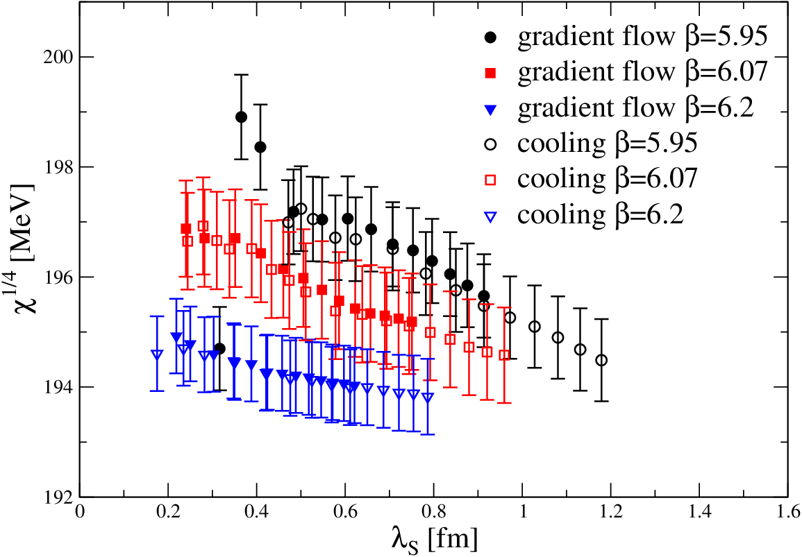
A nice scaling of the topological susceptibility to the continuum limit is observed in both cases (i.e. both for cooling and the gradient flow), see Figs. 7-8 for the case of the gradient flow, with extended plateaux around MeV, even if an accurate estimate of the finite size and UV cutoff systematic effects is not the purpose of this study.
| 5.95 | 6.07 | 6.2 | |
|---|---|---|---|
| 10.91(17) | 4.644(83) | 1.998(30) | |
| 10.91(18) | 4.653(84) | 1.999(30) | |
| 10.68(17) | 4.554(81) | 1.985(29) | |
| 10.74(17) | 4.566(82) | 1.987(29) |

III.4 Comparison configuration by configuration
We have shown that cooling and the gradient flow provide perfectly equivalent results for average topological quantities, such as the topological susceptibility. Here we want to make a more stringent test, comparing the outcome of the gradient flow and of cooling configuration by configuration.

First, we have determined the percentage of configurations where cooling and the gradient flow obtain different results for the global topological content . This is reported in Fig. 9: the topological charges were estimated after cooling steps and after units of flow time, respectively, however results are stable in a wide range of . The percentage is around 40% on the coarsest lattice () and it rapidly decreases, seemingly exponentially in , reaching around 1% on the finest lattice ().
One could suspect that this strong decrease is related to the variation of the physical volume; however, the effect of the volume change is in fact just a small contribution to this decrease. To check this point, we have performed simulations on a lattice at bare coupling (which is approximately of the same physical size as the lattice with ) and we have found that the percentage of configurations on which cooling and the gradient flow do not agree in the determination of is about . Therefore, also at constant volume this quantity strongly decreases with the lattice spacing.
It is interesting to compare this rate of different determinations of with the analogous rate obtained by comparing two slightly different versions of cooling, the one used in this paper and a simple variation, in which we just move the starting point of the cooling sweep from the origin to the middle of the lattice. Results are reported in Fig. 9 as well, and are completely equivalent with the previous ones, showing that the differences between cooling and the gradient flow are perfectly explainable in terms of the normal variations between different smoothing techniques, which take place when the starting configuration presents some degree of coarseness and rapidly disappear as one approaches the continuum limit.


A slightly different question is how much the different determinations of between the two methods are relevant with respect to the global topological activity, taking place on a given lattice at a given value. In order answer this question, we have measured the quantity
| (19) |
where and are the corresponding (i.e. at ) estimates of the topological charge obtained by cooling and by the gradient flow, and we have normalized it by the corresponding value of : in this way we normalize with respect to possible variations of the topological activity due, for instance, to the different physical volumes. Numerical results for are shown in Fig. 10: also in this case it is clear that the differences rapidly disappear as one approaches the continuum limit.
Finally, it is interesting to ask whether the observed agreement between cooling and the gradient flow is something that regards only the global topological charge of gauge configurations, or whether the agreement holds true also at a local level. The latter, of course, is a much stronger statement. In Fig. 11 we report the topological charge density, projected on the plane, obtained on a typical configuration where (with , and ). As one can appreciate, the agreement is also very good also at a local level. Such a result may give hints that for observables not directly related to topology one could also obtain similar results when adopting cooling or the gradient flow; however, a systematic investigation of this possibility is left to future studies.
IV Discussion and conclusions
The purpose of this study was to compare the gradient flow and the discrete flow generated by standard cooling, with respect to the determination of the topological properties of non-Abelian gauge theories on a lattice, with particular reference to the case of the pure gauge theory.
To that aim, we have first established a relation between the gradient flow time and the number of cooling steps , so that the plaquette action density, which is the quantity minimized by both flows, coincides. The relation holds within a good precision and already after a few cooling steps; such a relation is also in agreement with a perturbative estimate, which is expected to be valid in the limit of smooth fields and to depend on the dimensionality of the system ( where is the number of space-time dimensions), but not on the details of the gauge group.
We have proven that, after a very few transient cooling steps, the two flows lead to equivalent results, the transient region rapidly decreasing as the continuum limit is approached. This assertion is true at various degrees of strength. It is true for average quantities: we have checked this assertion with some accuracy for the topological susceptibility; however, given the superposition of the two probability distributions (see Fig. 3), we expect this to be true also for the higher order moments, which are needed to specify the dependence of the theory [27, 28, 29, 30, 21]
This expectation is also supported by the fact that, at a stronger level, even the discrepancies in the determination of , which are found configuration by configuration, rapidly become irrelevant as the continuum limit is approached, and already for fm. Moreover, the local profiles of topological charge densities, obtained by the two smoothing methods on sample configurations, are also very close to each other.
It is important, at this point, to stress that these conclusions do not depend on the specific prescriptions adopted to define the lattice topological charge or to perform the continuum limit. The outcome of this study is that, at every fixed lattice spacing, cooling and gradient flow give the same result provided the number of cooling steps and the flow time are related by (or, equivalently, the smoothing cutoff is chosen according to Eq. (13) and Eq. (14)).
Given the equivalence of the two procedures from a practical point of view, and at least regarding topological quantities, the choice of the method to be used in future simulations relies on the computational efficiency.
While for some applications the computational cost of both cooling and the gradient flow is negligible (like, e.g., for scale setting by the parameter [13]) there are cases in which this is not true. As a typical example we mention the evaluation of the higher momenta of the topological charge and, in particular, the computation of the renormalization group invariants commonly denoted by (see, e.g., [21]), whose determination requires independent determinations of . This makes even the pure gauge simulations far from trivial and the computational efficiency of the method used to estimate the topological charge becomes a crucial ingredient.
In particular, using the established relation , we can compare the execution time of three cooling steps with the time needed to perform an unity of gradient flow time evolution, obtaining . Clearly these estimates depend on the specific integrator adopted for the gradient flow and, in particular, adaptive integrators make it possible to obtain an speedup with respect to the third order RK solver (see Refs. [31, 32]). Nevertheless, cooling remains about one order of magnitude cheaper than the gradient flow.
Of course, one should consider that the gradient flow has advantages with respect to techniques like cooling, related to the fact that it has an associated differential equation, which clearly appear whenever an analytical treatment of the smoothing process is required, like, for instance, in the analysis of the renormalization properties of the smoothed fields [19]. Moreover, the gradient flow can be consistently extended to the presence of dynamical fermion fields [33]. We refer to [20] for a recent review of present and future perspectives of the gradient flow.
Finally, given the agreement of the topological charge density also at a local level, in the future one should better investigate the relation between the two smoothing procedures for other physical quantities as well.
Acknowledgments
We thank A. Di Giacomo, M. Mesiti, F. Negro, F. Sanfilippo and E. Vicari for useful discussions. Numerical simulations have been performed on the CSNIV cluster at the Scientific Computing Center at INFN-Pisa.
Appendix A A simple diffusive model
Let us consider a massless real scalar field, , on a three dimensional isotropic cubic lattice, where , and with the associated action
where runs over the three positive directions and indicates, as usual, the lattice site which is the nearest neighbor of in the forward direction. We will now consider the gradient flow for such a theory, and the differential equation obtained by it in the limit of smoothly varying fields. Then we will do the same in the case of cooling, and compare the two differential equations.
The gradient flow is defined by adding a dependence of on a fictitious time and letting
| (20) | |||||
In the limit of smoothly varying fields, we can take a continuum description and, letting , where is the lattice spacing, change the notation . The field on nearest neighbor sites can be Taylor expanded
so that the flow equation, Eq. (20), takes the simple form of a diffusive (heat) equation:
| (21) |
where is the 3D Laplacian operator.
Let us now consider cooling, in which the field is evolved by local minimization steps, which are iterated by sweeping all lattice sites at each cooling step. Let us call the field obtained after steps. If the lattice sites are visited in the positive lexicographic order, then it is easy to verify that the cooling equation is
| (22) |
where we have taken into account that part of the nearest neighbor sites have already undergone the cooling step under consideration. In order to write a corresponding differential equation, we now consider that, in the limit of smoothly varying fields, the evolution generated by cooling is also smooth, so we can Taylor expand in terms of a cooling timeas well, defined by , where is a fictitious temporal spacing that will be eventually set to 1. We can therefore substitute
We notice that, since we are dealing with a diffusion process, in which spatial distances scale like the square root of the diffusion time, it is consistent to Taylor expand at the linear order in time and at the quadratic order in spatial derivatives. Putting everything together, Eq. (22) becomes
| (23) |
which after setting teaches us that the relation between the cooling time and the gradient flow time is
meaning that 3 cooling steps correspond to 1 unit of gradient flow time. It should be clear that the factor 3 would have been a factor 6, had we not taken into account the additional cooling time dependence of half of the nearest neighbor fields.
References
- [1] K. G. Wilson, Phys. Rev. D 10, 2445 (1974).
- [2] M. Campostrini, A. Di Giacomo and H. Panagopoulos, Phys. Lett. B 212, 206 (1988).
- [3] P. Di Vecchia, K. Fabricius, G. C. Rossi and G. Veneziano, Nucl. Phys. B 192, 392 (1981); Phys. Lett. B 108, 323 (1982).
- [4] M. Teper, Phys. Lett. B 232, 227 (1989).
- [5] M. Campostrini, A. Di Giacomo H. Panagopoulos and E. Vicari, Nucl. Phys. B 329, 683 (1990).
- [6] A. Di Giacomo and E. Vicari, Phys. Lett. B 275, 429 (1992).
- [7] B. Allés, M. Campostrini, A. Di Giacomo, E.Vicari and Y. Gündüç, Phys. Rev. D 48, 2284 (1993) [hep-lat/9302004].
- [8] F. Farchioni and A. Papa, Nucl. Phys. B 431, 686 (1994) [hep-lat/9407026].
- [9] B. Allés, M. D’Elia and A. Di Giacomo, Nucl. Phys. B 494, 281 (1997) [Erratum-ibid. B 679, 397 (2004)] [hep-lat/9605013]; Phys. Lett. B 412, 119 (1997) [hep-lat/9706016]; Phys. Lett. B 483, 139 (2000) [hep-lat/0004020]; Phys. Rev. D 71, 034503 (2005) [hep-lat/0411035].
- [10] B. Allés, M. D’Elia, A. Di Giacomo and R. Kirchner, Phys. Rev. D 58, 114506 (1998) [hep-lat/9711026].
- [11] B. Berg, Phys. Lett. B 104, 475 (1981); Y. Iwasaki and T. Yoshie, Phys. Lett. B 131, 159 (1983); S. Itoh, Y. Iwasaki and T. Yoshie, Phys. Lett. B 147, 141 (1984); M. Teper, Phys. Lett. B 162, 357 (1985); E. -M. Ilgenfritz et al., Nucl. Phys. B 268, 693 (1986).
- [12] M. Luscher, Commun. Math. Phys. 293, 899 (2010) [arXiv:0907.5491 [hep-lat]].
- [13] M. Luscher, JHEP 1008, 071 (2010) [arXiv:1006.4518 [hep-lat]].
- [14] C. Morningstar and M. J. Peardon, Phys. Rev. D 69, 054501 (2004) [hep-lat/0311018].
- [15] M. Campostrini, A. Di Giacomo, H. Panagopoulos and E. Vicari, Nucl. Phys. B 329, 683 (1990).
- [16] M. Garcia Perez, O. Philipsen and I. -O. Stamatescu, Nucl. Phys. B 551, 293 (1999) [hep-lat/9812006].
- [17] J. E. Hetrick and P. de Forcrand, Nucl. Phys. Proc. Suppl. 63, 838 (1998) [hep-lat/9710003].
- [18] N. Cabibbo and E. Marinari, Phys. Lett. B 119, 387 (1982).
- [19] M. Luscher and P. Weisz, JHEP 1102, 051 (2011) [arXiv:1101.0963 [hep-th]].
- [20] M. Luscher, [arXiv:1308.5598 [hep-lat]].
- [21] E. Vicari and H. Panagopoulos, Phys. Rept. 470, 93 (2009) [arXiv:0803.1593 [hep-th]].
- [22] M. Guagnelli, R. Sommer and H. Wittig [ALPHA Collaboration], Nucl. Phys. B 535, 389 (1998) [hep-lat/9806005].
- [23] M. Creutz, Phys. Rev. D 21, 2308 (1980).
- [24] A. D. Kennedy and B. J. Pendleton, Phys. Lett. B 156, 393 (1985).
- [25] M. Creutz, Phys. Rev. D 36, 515 (1987).
- [26] B. Allés, L. Cosmai, M. D’Elia and A. Papa, Phys. Rev. D 62, 094507 (2000) [hep-lat/0001027].
- [27] L. Del Debbio, H. Panagopoulos and E. Vicari, JHEP 0208, 044 (2002) [hep-th/0204125].
- [28] M. D’Elia, Nucl. Phys. B 661, 139 (2003) [hep-lat/0302007].
- [29] L. Giusti, S. Petrarca and B. Taglienti, Phys. Rev. D 76, 094510 (2007) [arXiv:0705.2352 [hep-th]].
- [30] C. Bonati, M. D’Elia, H. Panagopoulos and E. Vicari, Phys. Rev. Lett. 110, 252003 (2013) [arXiv:1301.7640 [hep-lat]].
- [31] P. Fritzsch and A. Ramos, JHEP 1310, 008 (2013) [arXiv:1301.4388 [hep-lat]].
- [32] P. Fritzsch and A. Ramos, arXiv:1308.4559 [hep-lat].
- [33] M. Luscher, JHEP 1304, 123 (2013) [arXiv:1302.5246 [hep-lat]].