Testing the Clauser-Horne-Shimony-Holt inequality using observables with arbitrary spectrum
Abstract
The Clauser-Horne-Shimony and Holt inequality applies when measurements with binary outcomes are performed on physical systems under the assumption of local realism. Testing such inequalities in the quantum realm usually involves either measurements of two–valued quantum observables or pre-defining a context dependent binning procedure. Here we establish the conditions to test the Clauser-Horne-Shimony and Holt inequality using any quantum observable. Our result applies to observables with an arbitrary spectrum and no prior knowledge of their underlying Hilbert space’s dimension is required. Finally, we demonstrate the proposed general measurement strategy, that can be seen as positive operator valued measurements performed on the system, using the formalism of modular variables applied to the transverse degrees of freedom of single photons.
I Introduction
The Bell inequality was derived in 1964 [1] in response to the A. Einstein, B. Podolski and N. Rosen paradox [2], attempting to answer to the question: can quantum-mechanical description of physical reality be considered complete? By using the hypotheses of locality and realism, as used in [2], J. S. Bell, and later on, J. Clauser, M. Horne, A. Shimony and R. Holt (CHSH) [3] could establish an inequality that must be observed for measurements with binary outcomes performed on classical systems, even when one admits the hypotheses of local hidden variables (LHV) evoked in [2]. The interest of the CHSH inequality compared to the original Bell inequality is that it is easier to be tested experimentally, as demonstrated using quantum two–dimensional systems, such as the polarization of a photon [4] or spin systems [5]. The violation of the CHSH inequality can also serve as a benchmark for the quality of the entanglement produced by two–dimensional systems [7, 6].
The CHSH inequality involves correlations between measurements by two observers, and that can be expressed in terms of probabilities of obtaining two outcomes . It was shown in [8, 9] that this two valued binning, naturally present when observables with only two possible eigenvalues are measured, is essential in the derivation of the CHSH inequality. Measuring and manipulating multi-valued and continuous quantities can also lead to inequalities testing the possibility of LHV theories to explain non-locality [10, 11, 12], but these are not the scope of the present work.
In the present paper, we address the following problem: what are the conditions an observable must satisfy to be used in a test of a CHSH inequality, which can be violated for some particular quantum states showing that quantum correlations are stronger than those arising form LHV theories?
This paper is organized as follows: in section II we recall the CHSH inequality and then move to the main result of this paper, showing that any observable can be used to test a CHSH inequality. Our results can be interpreted using Positive Operator Valued Measurements (POVM) for each observer, naturally creating a binary statistics that can be used to test, and for some states, violate, a CHSH inequality. We then discuss in section III how our results can be used to test the CHSH inequality with no prior knowledge of the dimensionality of the Hilbert space of the measured observable. Section IV is devoted to a demonstration of the proposed measurement strategy using the formalism of modular variables applied to transverse degrees of freedom of single photons. Finally, we conclude in Sec. V.
II The CHSH Inequality
In the CHSH inequality, two physical quantities, and , are measured by observers and in different experimental settings where determines a setting and . To create a different experimental setting, some parameter of the experiment is modified, without altering the fact that only two values, , can be assigned to the measured quantity. The correlations appearing in the CHSH inequality are in the form:
| (1) |
where is the joint conditional probability that and observe the value when and are measured in the -th setting. These joint probabilities fulfill the normalization condition , for all settings ,.
Using (1), the CHSH inequality can be written as:
| (2) |
It was shown in [8, 9] that the CHSH inequality demands that the statistics of the measurement outcomes of and are associated to some two–valued binning. By such, we mean that it is mandatory that correlation functions can be written as in (1), which is a direct consequence of the fact that, for each party, the expectation value of, say, can be written as , where and .
In the quantum formalism, the physical quantities and become hermitian operators (observables): and . The first observables that appeared as natural candidates to test Eq. (2) were quantum two-dimensional ones, that can be constructed from the three Pauli matrices, , . Measurement of the Pauli operators in any direction of space can only return the values with some probability that can be directly associated to the probability of obtaining one of the two eigenstates of (or ).
Less intuitive examples of two–valued observables that can be measured for states in Hilbert spaces of higher dimensions can be constructed by dichotomization [13, 15, 14, 16, 17]. This strategy allows the testing and violation of the CHSH inequality using a two-valued binning of experimentally accessible continuous variable measurements. One example of a dichotomic observable is the displaced parity operator whose expectation value can be directly associated with the Wigner function [13, 18, 19, 20]. Furthermore, a test of the CHSH inequality for high dimensional discrete and continuous systems was proposed in [16] by binning local measurement outcomes. The same authors generalized the parity-based approach in [13] in order to test the CHSH inequality in terms of a parametrized set of quasiprobability functions including the Wigner function as limiting case. Another state-dependent binning procedure was proposed in [21] by assigning binary probabilities to continuous measurement outcomes lying in some pre-defined regions of the phase space. Finally, in [22], a measurement strategy based on auxiliary two-level systems was devised to transfer information of continuous variables states to observables with a two–valued spectrum.
The above strategies to test the CHSH inequality aim at explicitly identifying to probabilities of projective measurement outcomes. However, this leads to excessively restrictive conditions to observables or , that are required to have specific spectral properties. Such restrictions not only reduce the space of states that can violate a CHSH inequality but also the possible experimental set-ups that are suitable to test it.
From the experimental point of view the ideal situation would be as follows: suppose that observers, and are capable of measuring observables and with an arbitrary spectrum that is not necessarily known; is it possible to design a strategy for and to test a CHSH inequality using measurements of such observables, without resorting to dichotomization or to a binning procedure? We show that it is indeed possible to test a CHSH inequality using observables with an arbitrary spectrum if one realizes that equation (2) merely involves binary correlations between measurement results, and only the expectation values of observables are relevant, not their spectrum. This possibility is interesting not only because it renders CHSH inequality tests accessible to any experimental set-up, but also because it helps designing loophole-free experimental tests the CHSH inequality.
In order to obtain a binary statistics in the quantum realm, requiring that observables and have a two-valued spectrum is a too strong demand, since (2) involves probabilities only. Testing (2) demands designing experiments simply reproducing the same type of statistics as in (1) but such experiments can, in principle, involve systems with an arbitrary Hilbert space dimension. Thus, observables and must merely be such that
| (3) |
. A combination of four such values with different settings (), as in (2), leads to a violation of the inequality (2) for some entangled quantum states . We will see that the condition such observables must satisfy does not necessarily require a known a priori binning process, and that the previous cited examples of two–valued observables are particular cases of the general operators we obtain.
We start by considering a single party operator, and the same reasoning will be applied to . Since our basic requirement is that with , there exists a such that , and . Meaning that, if we are able to measure an arbitrary observable , with eigenstates defined as and eigenvalues such that , we can construct any unitary operator , where is an arbitrary function and is the projector onto the eigenspace associated to a value of . In the present paper, for simplifying reasons, we will focus on the case where . We thus define the real part of as:
| (4) |
In (4) we considered the most general case, where has a continuous spectrum. Operators with a discrete spectrum can be written in a form analogous to (4) by replacing the integral by a sum over the discrete eigenstates of . For instance, Pauli matrices are a particular case of (4). In this case, there are only two eigenstates , , with eigenvalues . For any value of , a proper normalization recovers the Pauli matrices with spectrum .
Our results can be interpreted in terms of a two valued POVM, , such that
| (5) |
Indeed, since the spectrum of is in , are positive operators, and by construction, and . Therefore the probabilities fulfill the required relations : and . Using Eq. (4), we have that and the POVM can thus be written as:
| (6) |
while the case of binary projective measurements is recovered when is hermitian. Correlations between the outcomes of measurements of and in the form (4) can be constructed as:
| (7) |
, directly leading to (3), without the need of a prior choice of a binning procedure, dramatically simplifying experimental tests of the CHSH inequality. This formulation is a special case of the more general fact that the expectation value of any bounded observable can be expressed in terms of a binary POVM [41].
Considering such general form is interesting because it opens the perspective of testing CHSH inequalities in any measurable quantum system: once one knows how to measure the probability of finding a quantum system in the eigenstates of an arbitrary measurable observable , operators as (4) can be constructed, leading to the test of a CHSH inequality using (7). In many experimental systems, it appears that projective measurements are not accessible. In [23] it was suggested that parity measurements [13] could lead to violation of the CHSH inequality. However, the state of the art of this set-up is far from enabling such projective measurements [24], and only POVMs are accessible.
A consequence of the presented results is that knowing the general form (4) allows testing a CHSH inequality with no a priori information about the Hilbert space dimension of the system to be measured and on possible binning or dichotomization procedures. By measuring an observable in the form (4) in some experimentally accessible basis , one is sure to be able to test a CHSH inequality without requiring any other information about the system. This point will be further discussed in the next section, where we consider a situation where one does not know, a priori, the Hilbert space dimension of the measured observable.
III Illustration using measurements performed to observables of unknown dimension
In order to illustrate this fact and the power of our results, we consider the following situation: suppose that each one of the observers and has a measuring apparatus that correlates some physical property of a quantum system to its position and then measures it. The measurement of the referred quantum property is thus indirectly performed by collecting statistics about the quantum system’s position. This scenario is probably the most current in physics, corresponding to Stern-Gerlach (SG) type experiments [25], measurements of the spectrum of a multi-mode field using a diffraction grating, the Mach-Zehnder interferometer, among many others. If the referred physical property is associated to an observable with unknown dimension, as was the case of the first SG experiment, no assumption can be made, a priori, on the possible outcomes of the position measurements. In order to be even more general, one can suppose that the way correlations are created between position and the physical quantity to be measured is also unknown. Thus, observers and , when inspecting the position probability distribution that is measured by their apparatuses, have simply no idea of what type of results they can find. Using the present formulation, even in this extremal case, there exists a strategy enabling, in principle, the violation of the CHSH inequality (2).
This scenario can be expressed mathematically as follows: we consider first the case of a single party system and then extend our results to the bipartite case. The initial state of the system is given by
| (8) |
where is a complete basis describing the property that is being measured. is the position measurement result when no correlation is created between position and some property of . In the case of a SG experiment, for instance, would be the different projections of the spin into a given axis. Before the realization of this experiment, it was believed that this quantity could assume a continuity of values, and the description in (8) is the most general one in this case. Of course, after the SG experiment, a specific discrete form was inferred for . Starting from (8) we create correlation between position and some property of , that will be labeled . The system’s state becomes:
| (9) |
where and . In order to illustrate (9) we can think of the example of perfect correlation between position . In this case, . This situation describes the SG experiment or diffraction by a grating. Another situation would be the one of parity measurements, i.e., when position becomes correlated to the parity of the state. Then, by writing , where are the odd/even parts of , the system’s state is split in two according to its parity, and there are only two states : . Correlations between parity and position can be created in optical systems, for instance, by using an orbital angular momentum sorter [26]. The previous cases are extreme examples, illustrating either perfect or binary correlation. Both extremes, and all the intermediate cases are covered by the present formalism, even of one does not know what type of correlations are created between position and some property of the system. Since and are realizing position measurements, in order to be able to test (2), they can use an operator as (4) in the position basis, irrespectively of the type of information position measurements bring from the quantum system.
An example of an unitary operator in the position basis is , where is some number with the dimension of a length. is infinitely degenerated, since its eigenvalues are periodic. The integral over the whole space can be replaced by an integral over one period and an infinite sum if one defines the following notation: let and [27]. Then, can be written as:
| (10) |
By identifying with , we have that
| (11) | |||||
where [28]. This is an example of an observable in the form (4) in the position basis that can reveal the binary statistics required for testing CHSH inequalities. We now compute its expectation value using the general state (9). For this, we re-express (9) using that , leading to
| (12) |
where and the limit of the sum can in principle go to infinity. Expressions analog to (12) can be created to and . However, in this last case, one would have to compute the coincidence position measurements of and . In this bipartite case, the initial state is
| (13) |
where is the position of the particle detected by observer . Following the same principles as before, correlations between position and the physical quantities measured by and are given by:
| (14) |
where and . We can thus write
| (15) |
where [29]. We can notice that the presented results are quite general and do not depend on the specific form of the function , describing how correlations between the observable to be measured and position are created.
Eq. (15) corresponds to an arbitrary experimental setting . In (2) one must be able to change settings and compare correlations between the measurement results in different settings. This can be done by applying an unitary operation to the measurement apparatus, which is formally equivalent to applying it to the initial state while keeping the measurement apparatus unchanged. Correlations between measurements in different settings can be combined, as in (2), so as to test the CHSH inequality for a system whose Hilbert space dimension is unknown. In this scenario, if one supposes that observers blindly compute the quantity (15) for each setting without necessarily observing the statistics of position measurements in detail, it would be possible to violate the CSHS inequality without discovering that the spin projections are two-valued quantities, in the case of a SG experiment.
We now discuss a specific example, showing how measurements on the transverse degrees of freedom of photon pairs can be handled using our ideas so as to lead to the violation of the CHSH inequality.
IV Example: CHSH inequality violation using the transverse degrees of freedom of photons
IV.1 Modular variables formulation
We illustrate our recipe for testing CHSH inequalities in arbitrary dimensions using the formalism of modular variables [27, 28]. Therefore, we split the position and momentum operator into a discrete and a modular part:
| (16) |
where () has integer eigenvalues, and () represents the modular position (momentum) operator with eigenvalues (). As in Sec. III, is an arbitrary length scale that can be chosen later on according to some property of the physical system under consideration. Since the modular position and momentum operator commute [27], we can define a common set of eigenstates , referred to as modular eigenstates. In the following, we will express all operators and states in terms of the modular basis.
In order to test the CHSH inequality using the position measurements, as exemplified in Sec. III, we use the operator (11) which, in the modular basis, reads:
| (17) |
where . Furthermore, to specify different measurement settings we define the transformed operator , using the continuous set of unitaries . Specifically, by choosing , we get:
where . Now, according to Sec. II, we use the operators (17) and (IV.1), to define the Bell operator:
| (19) |
where we used capital letters to distinguish between system and . Candidates of states for which the expectation value the operator (19) violates the local-realism threshold of can be found by diagonalizing the operator , in the basis , where . This yields two nonzero eigenvalues and the corresponding eigenvectors:
| (20) |
where . These nonnormalizable states violate the CHSH inequality maximally for the choice and , yielding . Furthermore, we can construct physically meaningful states that still yield a large amount of violation by continuously superposing the states in Eq. (20) with localized wave packets centered sufficiently near to the positions for which the maximum violation occurs. An example of such a state is:
| (21) |
where are normalized wave packets with support contained in . We note, that the wave function on the whole modular space , is not equal to , but according to Eq. (21) also involves the definition of . In the following, we use, as example, the wave function of spatially entangled photon pairs that have passed through diffraction gratings. As we will show in the Sec. IV.2, such a wave function can, in the modular representation, be represented by a product of two Gaussians together with periodic boundary conditions on the domain :
| (22) |
where and denote the width and position of the wave function in the modular position and momentum.
In Fig. 1, we present numerical results of as a function of , for different values of the parameters , and , showing the violation of the CHSH inequality. We see that, in the case of an infinitely squeezed modular momentum contribution () centered at (see Fig. 1(a)), the maximum of passes the local-realism threshold if , and approaches the value of maximal violation () in the limit . Indeed, if we choose we get , and thus . Further on, for finite values of the modular momentum width and position (see Fig. 1(b)), the maximum of is reduced but still violates the threshold if . The asymmetry of with respect to , in Fig. 1(b), originates from the dependency of the cosine in Eq. (IV.1) which in the former case (see Fig. 1(a)), for and , does not play a role.

In the next Section, we will outline how the above described Bell test can be performed experimentally using measurements on the transverse degrees of freedom of photon pairs.
IV.2 Proposal of experimental implementation using the transverse degrees of freedom of photon pairs
The mathematical structure of the spatial multimode field of a single photon reveals a perfect analogy with that of a single mode of the electromagnetic field containing a large number of photons [37]. In particular, due to the richness of optical elements and devices available in state of the art quantum optics experiments, the transverse degrees of freedom of a photon are an interesting playground for the implementation of quantum information applications [44, 43]. In this section, we employ the transverse degrees of freedom of photon pairs in order to implement the above described test of the CHSH inequality (see Sec. IV.1).
IV.2.1 Measurement of observables
In the paraxial approximation it is convenient to describe the spatial degrees of freedom of a single photon state by a transverse wave function providing the probability amplitude for the detection of the photon in the transverse plane [37]. Moreover, it is possible to implement, on this transverse space, a universal set of unitary gates allowing for the approximate construction of all unitary operations by concatenating these gates. In order to construct the operators (17) and (IV.1) we only need two unitary operators from the basic set of continuous unitary gates [36]. Namely, the momentum shift operator , and the single photon propagation , where and represent the transverse position and momentum operators of one of the two orthogonal transverse dimensions of the single photon, respectively. By combining and , we can define the operators:
| (23) | ||||
| (24) |
where we set and . Single unitaries, and , can be implemented straightforwardly using linear optical elements and the free propagation of the photons [37]. However, for the sum of two unitaries one needs to employ an additional degree of freedom as the polarization of the photons, or their propagation direction, that can be, for instance, the two paths of an interferometer. In Fig. 2, we demonstrate how the expectation value of the operators (23) and (24) can be measured using a Mach-Zehnder interferometer setup, as discussed in previous works [38, 39]. We will see that this can be done by simply counting the arrival of photons in the outputs of the interferometer yielding the corresponding photon count probabilities:
| (25) |
with , and hence:
| (26) |
Note that the interferometers simply serve as strategy allowing the performance of the corresponding POVM’s, (compare with Eq. (6)), on the transverse field of the photons. Further on, the measurement of the products , as required in the CHSH inequality, can be preformed in an equivalent manner, using two analogous Mach-Zehnder interferometers, by counting the photon coincidences in the four outputs of the two interferometers, leading to the coincidence probabilities , with the two-partite POVM (see also Eq. (7)):
| (27) |
for .
IV.2.2 Preparing spatially entangled states
Next, we explain how entangled states as (21) can be produced experimentally using the spatial degrees of freedom of photon pairs. For that, we first show how to engineer single photon states in the form or , with chosen according to Eq. (22).
Let us consider the transverse wave function of a single photon directly after it has passed through an infinitely extended diffraction grating with slit distance [42]:
| (28) |
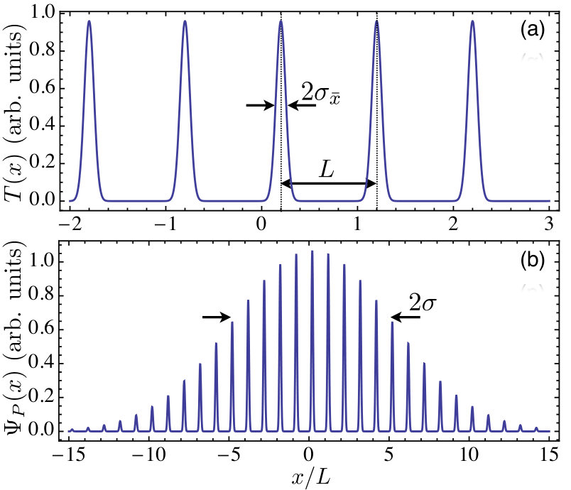
Here, is the -periodic grating transmission function, defined through the Fourier coefficients , such that , and a Gaussian with width accounting for the finite extension of the single photon wave packet. An example of and , for , is shown in Fig. 3(a) and (b), respectively. We see that, for this choice of the coefficients , represents a comb of Gaussians with width , and a Gaussian envelope thereof.
Further on, if we assume the approximation becomes permissible and Eq. (28) transforms to the modular representation as:
| (29) |
where we set , is defined by restricting to the domain and represents a comb of Gaussians in momentum space with width restricted to the domain . Equation (29) is thus nothing but the product of two Gaussians with width and , respectively, and periodic boundaries on the domain (compare with Eq. (22)). Hence, by tuning the parameters and , we are able to generate the states or . Thereby, the theoretical limit , as assumed in the calculations leading to the results presented in Fig. 1(a), of an infinitely squeezed modular momentum (see Eq. (22)), corresponds to the idealized situation of an infinitely extended single photon transverse wave function ().
Experimentally, the ratio of can be modified by adjusting the slit width and distance of the diffraction grating that is used to create the interference pattern. The transverse location of the grating can be associated to the position of the interference peaks of the photon’s wave function (28) with respect to its envelope (see Fig. 3(b)), and thus to the value of . And finally, a nonzero mean modular momentum , as assumed in Fig. 1(b), can be achieved by imprinting a position dependent phase , with , on the transverse field of the photon (28). The latter is readily realized using a spatial light modulator (SLM) whose action on the photon’s transverse wave function can be described as with a user-defined function .
Now, knowing how to prepare the single photon states and , we can use a technique that was previously proposed in [40], in order to create the spatially entangled state (21) of a photon pair. To this end, we first use spontaneous parametric downconversion to produce a polarization entangled state , by pumping two adjacent nonlinear crystals (type I) with a laser beam polarized at , and, subsequently, bring it into the form:
| (30) |
where , by the correct application of local unitary transformations on each of the entangled photons, realized by combinations of half- and quater-wave plates, as shown in Fig. 4. Thereby, the transverse wave function of the two photons remains in the separable Gaussian state . Next, we have to swap the entanglement from the polarization to the transverse degrees of freedom of the photons according to and . This swapping is realized experimentally using an interferometer with polarizing beam splitters (see Fig. 4), such that, depending on the polarization of the photons, the operation or , with the help of single photon diffraction gratings, can be performed. One of the two photons must be rotated before entering the interferometer, in order to assure that initially H-polarized -photons will go through the same arm of the interferometer as H-polarized -photons. Finally, one uses half-wave plates oriented at in the path of both photons and polarizing beam splitters in order to factorize the polarization from the transverse degree of freedom yielding the desired state (21) conditionally with a probability.
V Discussion and Conclusion
We now discuss the natural binning procedure that is realized by the operator (4). Consider the eigenstates with maximum (minimum) eigenvalue of the observable , denoted as . In a realistic situation such states have a normalizable wave function with nonzero width , which lead, in the limit , to the expectation value . When considering quantum systems of arbitrary dimension, it is clear that, due to degeneracies, an infinity of states, to which we refer to as , can lead to the same value of . These states are associated to the same expectation value , and can be regarded equivalent as far as this quantity is concerned. In this sense, they are also equivalent to a state , where is an arbitrary phase, such that
| (31) |
Simple examples of such states are , where is an integer. These results can be straightforwardly extended to the correlations .
In conclusion, we provided the general conditions observables with an arbitrary spectrum must satisfy to be suitable to test a CHSH type inequality. We have shown that dichotomic observables are a particular case of the formal solution developed here. We also detailed the situation where observers have access to position measurements only and position is correlated in an unknown way to some physical property of the system to be measured. Our results help creating a general environment for CHSH inequalities tests without the need of complicated state dependent binning procedures or prior knowledge of the physical properties of the system, rendering CHSH inequalities tests accessible to a broader class of experimental systems and significantly simplifying their realization. An interesting perspective is applying the same principles developed here to other type of inequalities valid under the assumption of local realism, as [10, 11, 12, 35].
Acknowledgements.
The authors acknowledge financial support by ANR/CNPq HIDE and ANR COMB. The authors are indebted to P. Grangier for inspiring discussions, and to P.H.S. Ribeiro, S.P. Walborn, J.-M. Raimond, M. Brune, J. Laurat and N. Treps for fruitful comments.References
- [1] J.S. Bell, Physics 1, 195 (1964).
- [2] A. Einstein, B. Podolsky, and N. Rosen, Phys. Rev. 47, 777 (1935).
- [3] J. F. Clauser, M. A. Horne, A. Shimony, R.A. Holt, Phys. Rev. Lett. 23 (15): 880 (1969).
- [4] A. Aspect, P. Grangier, and G. Roger, Phys. Rev. Lett. 49, 91 (1982).
- [5] M.A. Rowe, D. Kielpinski, V. Meyer, C.A. Sackett, W.M. Itano, C. Monroe, D.J. Wineland, Nature 409, 791 (2001).
- [6] G. Weihs, T. Jennewein, C. Simon, H. Weinfurter and A. Zeilinger, Phys. Rev. Lett. 81, 5039 (1998).
- [7] R. Horodecki, P. Horodecki, M. Horodecki, K. Horodecki, Rev. Mod. Phys. 81, 865 (2009).
- [8] A. O. Barut and P. Meystre, Phys. Lett. 105 A, 458 (1984).
- [9] A. Aspect, Frontiers of Non Equilibrium Physics, G. T. Moore and M. O. Scully, editors (1986).
- [10] E. G. Cavalcanti, C. J. Foster, M. D. Reid and P. D. Drummond, Phys. Rev. Lett. 99, 210405 (2007).
- [11] D. Collins, N. Gisin, N. Linden, S. Massar and S. Popescu, Phys. Rev. Lett. 88, 040404 (2002).
- [12] F. Arnault, J. Phys. A: Math. Theor. 45, 255304 (2012).
- [13] K. Banaszek, and K. Wódkiewicz, Phys. Rev. Lett. 82, 2009 (1999).
- [14] U. Leonhardt and J. Vaccaro, J. Mod. Optics 42, 5 (1995)
- [15] A. Gilchrist, P. Deuar, and M. D. Reid, Phys. Rev. Lett. 80, 3169 (1998).
- [16] S.-W. Lee and D. Jaksch, Phys. Rev. A 80, 010103 (2009).
- [17] S.-W. Lee, H. Jeong and D. Jaksch, Phys. Rev. A 80, 022104 (2009).
- [18] Z.-B. Chen, J.-W. Pan, G. Hou, G. and Y.-D. Zhang, Phys. Rev. Lett., 88, 040406 (2002).
- [19] T. Yarnall, A. F. Abouraddy, B. E. A. Saleh, and M. C. Teich, Phys. Rev. Lett. 99, 170408 (2007).
- [20] A. Kuzmich, I. A. Walmsley, and L. Mandel, Phys. Rev. Lett 85, 1349 (2000).
- [21] J. Wenger, M. Hafezi, F. Grosshans, R. Tualle-Brouri, and P. Grangier, Phys. Rev. A 67, 012105 (2003).
- [22] X.- F. Qian, C. J. Broadbent and J. H. Eberly, New Journal of Physics 16, 013033 (2014).
- [23] P. Milman, A. Auffèves, F. Yamaguchi, M. Brune, J.-M. Raimond and S. Haroche, Eur. Phys. J. D 32, 233 (2005).
- [24] S. Deléglise et al., Nature 455, 510 (2008).
- [25] W. Gerlach and O. Stern, Zeit. Phy. 9, 353 (1922).
- [26] J. Leach, M. J. Padgett, S. M. Barnett, S. Franke-Arnold, and J. Courtial, Phys. Rev. Lett. 88, 257901 (2002).
- [27] Y. Aharonov, H. Pendleton and A. Petersen, Int. J. Theor. Phys. 2, 212 (1969).
- [28] P. Vernaz-Gris, A. Ketterer, A. Keller, S.P. Walborn, T. Coudreau and P. Milman, Phys. Rev. A 89,052311 (2014).
- [29] In practical situations, position measurements are realized in a given finite interval defined as , even in the case where the spectra and are arguably infinite. We can thus set , which is equivalent to consider and and , that will simplify the notation and interpretation of the results.
- [30] T. Eberle, S. Steinlechner, J. Bauchrowitz, V. Händchen, H. Vahlbruch, M. Mehmet, H. Müller-Ebhardt, and R. Schnabel, Phys. Rev. Lett. 104, 251102 (2010).
- [31] J. Roslund, R. M. de Araújo, S. Jiang, C. Fabre and N. Treps, Nat. Phot. 8, 109 (2014).
- [32] A.S. Villar, L. S. Cruz, K. N. Cassemiro, M. Martinelli, and P. Nussenzveig, Phys. Rev. Lett. 95, 243603 (2005).
- [33] G. Ferrini, J. P. Gazeau, T. Coudreau, C. Fabre and N. Treps, New J. Phys. 15, 093015 (2013).
- [34] R. Horodecki, P. Horodecki and M. Horodecki, Phys. Lett. A, 200, 340 (1995).
- [35] A. Asadian, C. Brukner and P. Rabl, Phys. Rev. Lett. 112, 190402 (2014).
- [36] Samuel L. Braunstein, and Peter van Loock, Rev. Mod. Phys. 77, 513 (2005).
- [37] D. S. Tasca, R. M. Gomes, F. Toscano, P. H. Souto Ribeiro, and S. P. Walborn, Phys. Rev. A 83, 052325 (2011).
- [38] S. Machado, P. Milman, and S. P. Walborn, Phys. Rev. A 87, 053834 (2013).
- [39] M. Hor-Meyll, J. O. de Almeida, G. B. Lemos, P. H. Souto Ribeiro, and S. P. Walborn, Phys. Rev. Lett. 112, 053602 (2014).
- [40] C. V. S. Borges, A. Z. Khoury, S. Walborn, P. H. S. Ribeiro, P. Milman, and Keller, A., Phys. Rev. A 86, 052107 (2012)
- [41] P. Horodecki, Phys. Rev. A 67, 060101 (2003).
- [42] W. B. Case, M. Tomandl, S. Deachapunya, and M. Arndt, Opt. Express 17, 20966 (2009).
- [43] M. A. D. Carvalho, J. Ferraz, G. F. Borges, P. -L. de Assis, S. Pdua, and S. P. Walborn, Phys. Rev. A 86, 032332 (2012).
- [44] A. N. de Oliveira, S. P. Walborn and C. H. Monken, J. Opt. B 7, 288 (2005).