Steady-State Axisymmetric MHD Solutions
with Various Boundary Conditions
Abstract
Axisymmetric magnetohydrodynamics (MHD) can be invoked for describing astrophysical magnetized flows and formulated to model stellar magnetospheres including main sequence stars (e.g. the Sun), compact stellar objects [e.g. magnetic white dwarfs (MWDs), radio pulsars, anomalous X-ray pulsars (AXPs), magnetars, isolated neutron stars etc.], and planets as a major step forward towards a full three-dimensional model construction. Using powerful and reliable numerical solvers based on two distinct finite-difference method (FDM) and finite-element method (FEM) schemes of algorithm, we examine axisymmetric steady-state or stationary MHD models in Throumoulopoulos & Tasso (2001), finding that their separable semi-analytic nonlinear solutions are actually not unique given their specific selection of several free functionals and chosen boundary conditions. Similar situations of multiple nonlinear solutions with the same boundary conditions actually also happen to force-free magnetic field models of Low & Lou (1990). The multiplicity of nonlinear steady MHD solutions gives rise to differences in the total energies contained in the magnetic fields and flow velocity fields as well as in the asymptotic behaviours approaching infinity, which may in turn explain why numerical solvers tend to converge to a nonlinear solution with a lower energy than the corresponding separable semi-analytic one. By properly adjusting model parameters, we invoke semi-analytic and numerical solutions to describe different kind of scenarios, including nearly parallel case and the situation in which the misalignment between the fluid flow and magnetic field is considerable. We propose that these MHD models are capable of describing the magnetospheres of MWDs as examples of applications with moderate conditions (including magnetic field) where the typical values of several important parameters are consistent with observations. Physical parameters can also be estimated based on such MHD models directly. We discuss the challenges of developing numerical extrapolation MHD codes in view of nonlinear degeneracy.
Keywords:
magnetohydrodynamics (MHD) – magnetic fields – stars: neutron – white dwarfs – stars: winds, outflows – methods: numerical1 Introduction
Magnetohydrodynamics (MHD) is often invoked to describe dynamic motions of (fully or partially) ionized and magnetized plasmas in broad contexts of astrophysical systems. Since hydrodynamic equations for such a magnetized plasma are coupled with the Maxwell equations of electrodynamics (Jackson, 1975, e.g.), direct solutions to this set of MHD nonlinear partial differential equations (PDEs) are extremely challenging and notoriously complicated, which are usually obtained through numerical simulations. For favorable and special situations, when some additional conditions such as ideal MHD, steady state and spatial symmetries (especially the type of symmetries that can reduce the problem to a 2.5-dimensional one, e.g. helical symmetry, translational symmetry or axisymmetry) are assumed, the system of MHD PDEs can be significantly simplified after tedious yet straightforward algebraic and calculus manipulations (Tsinganos, 1981; Tsinganos, 1982a; Tsinganos, 1982b, e.g.). Vector nonlinear ideal MHD PDEs can be reduced to scalar ones by making use of available conservation laws and by considerable simplifications due to symmetries. There have been various attempts to construct semi-analytic nonlinear solutions under allowed conditions. The scenarios of those attempts range from static force-free cases (Low & Lou, 1990, e.g.) to MHD cases with dynamic flows (Low & Tsinganos, 1986; Khater et al., 1988; Tsinganos & Low, 1989; Contopoulos & Lovelace, 1994; Del Zanna & Chiuderi, 1996; Khater & Moawad, 2004; Throumoulopoulos et al., 2007, e.g.).
In this paper, we adopt the ideal MHD formulation and approach of Tasso & Throumoulopoulos (1998) and especially of Throumoulopoulos & Tasso (2001), in which axisymmetry and incompressible conditions are both imposed to further reduce the problem, while the gravitational field of a central stellar object and gas flows are retained for sensible physical reality. The idealizations and semi-analytic results form the key basis of our further numerical explorations and elaborations.
Those MHD PDEs are nonlinear, raising the possibility that their solutions may not be unique for a given set of specified boundary conditions in general. In the current context, this specifically relates to the important issue of boundary conditions at large radii for the extrapolation of solar and stellar coronal magnetic field configurations. By our independent numerical explorations using distinct finite-difference method (FDM) and finite-element method (FEM) schemes, we noticed that a class of separable semi-analytic solutions to the force-free magnetic field problem of Low & Lou (1990) are indeed not unique with the same nonlinear PDEs and spatial boundary conditions, which in fact substantially extended and confirmed the results of Bruma & Cuperman (1993) (see Appendix B for more details). A specific index in Bruma & Cuperman (1993) (see also Appendix B here) turns out to be critical for the presence of multiple nonlinear solutions with the same boundary conditions. When this is greater than a critical value , the solution is unique; when its value decreases such that , the solution “bifurcates” into two branches, even though the boundary conditions for the two solution branches remain identical. Mathematically, the type of quasi-linear MHD differential equation in Throumoulopoulos & Tasso (2001) may not be excluded for possibly possessing multiple solutions when the functional corresponding to the original PDE is not convex (see Taylor, 2011, for the pertinent functional analysis). These hints and clues motivate us to carefully examine the uniqueness of solutions by solving the nonlinear MHD PDEs numerically in reference to the available semi-analytical solutions. Numerical solvers implemented with quite different algorithms [e.g., FDM and FEM] and variable grid resolutions are applied to perform necessary mutual cross-checks, which would give us reasonable confidence on our numerical findings that a definite type of different numerical solutions may exist with the same boundary conditions and nonlinear MHD PDEs as in Throumoulopoulos & Tasso (2001).
Axisymmetric nonlinear ideal MHD PDEs are often invoked to describe a variety of astrophysical magnetized plasma systems, such as magnetized accretion discs, magnetized stellar winds, magnetized astrophysical jets on completely different scales (Lovelace et al., 1986; Low & Tsinganos, 1986; Khater et al., 1988; Tsinganos & Low, 1989; Contopoulos & Lovelace, 1994; Proga et al., 2003, e.g.), and magnetospheres of stars (e.g., the Sun), planets (e.g., Earth, Jupiter, Saturn etc.) and compact stellar objects (e.g., radio pulsars, magnetars, AXPs, isolated neutron stars, cataclysmic variables etc.) (Michel, 1973; Contopoulos et al., 1999; Komissarov, 2006). Compact stellar objects, including white dwarfs and neutron stars etc., possess intense magnetic fields as inferred by extensive observations. For neutron stars (e.g. radio pulsars, AXPs, magnetars, isolated neuron stars), whose magnetic field intensities may reach as high as , the so-called force-free conditions are often presumed since the magnetic Lorentz force can be hardly balanced by other known forces (such as gravity and pressure force). Meanwhile, velocity of magnetized fluid particles are usually so large that relativistic conditions could also apply (Lou, 1992; Lou, 1993a; Lou, 1993b; Lou, 1998; Spitkovsky, 2006, e.g.). However, for magnetic white dwarfs, the intensity of magnetic field is significantly lower around (Schmidt & Smith, 1995, e.g.), in which we would expect that the force-free condition may not hold and thus the misalignment between the fluid flow and magnetic field may possibly be considerable. We expect that, by properly selecting parameters, the semi-analytic MHD models of Throumoulopoulos & Tasso (2001) and our corresponding numerical models may offer reasonable though idealized descriptions for magnetospheres of magnetic white dwarfs (MWDs) in general.
This paper is structured as follows. Section 2 presents the basic model formulation of the simplified and reduced ideal MHD problem. Key steps in derivations and reductions of MHD PDEs to a single scalar PDE involving free functionals are shown in Section 3. In Section 4, semi-analytic solutions and their corresponding numerical model solutions are presented to compare with the pertinent computational results. Section 5 offers analyses and astrophysical applications of our ideal MHD models. We summarize results and conclusions in Section 6. Mathematical derivations are detailed in three Appendices for the convenience of reference.
2 Basic MHD Model Formulation
Steady-state (i.e. stationary or time-independent) ideal MHD is governed by the following set of nonlinear PDEs in c.g.s.-Gaussian units, which combine the Maxwell equations and the Eulerian hydrodynamic equations with certain approximations (Tsinganos, 1981, e.g.):
| (1) |
where is the unit vector along the radial direction pointing outwards, is the radius, is the fluid mass density, is the central stellar mass, is the plasma pressure, is the bulk flow velocity vector, and are the electric and magnetic vector fields respectively, is the speed of light, and is the universal gravitational constant. The ideal MHD approximation is adopted here to ignore effects of resistivity, viscosity, thermal conduction and radiative losses and so forth, while the gravitational field of a central spherical stellar object (e.g. a main-sequence star, a neutron star or a white dwarf) of mass is included. We shall not go into the stellar interior and thus regard the spherical stellar surface as the inner boundary denoted by a reference radius . The change of shape for the stellar surface due to rotation is ignored in the present treatment. In this formalism, we analyze pertient problems in spherical polar coordinates for radius , polar angle and azimuthal angle , respectively (n.b. the notations and introduced later bear different meanings than in our formalism). We use to denote the cosine of for the convenience of mathematical analysis.
We note a few basic invariance properties of stationary MHD PDE system (1) under several transformations. First, for a simultaneous transformation of to and to with other variables unchanged, MHD PDE system (1) remains invariant. Secondly, for a simultaneous transformation of to and to with other variables unchanged, nonlinear MHD PDE system (1) remains invariant. Thirdly, for a simultaneous transformation of to and to with other variables unchanged, MHD PDE system (1) remains invariant. These properties can be readily understood on intuitive physical terms for ideal MHD.
3 Derivation for steady ideal MHD PDEs with axisymmetry and incompressible fluid
The formalism in the foregoing section is sufficiently general. When axisymmetry and incompressibility are imposed, system (1) of nonlinear ideal MHD PDEs can be considerably simplified. In this section, we briefly review the simplification steps in Tsinganos (1982a); Tasso & Throumoulopoulos (1998) and especially Throumoulopoulos & Tasso (2001) (n.b. we have properly recast some pertinent expressions in c.g.s.-Gaussian units in a consistent manner). Details of derivations and reductions relevant to this section are included in Appendix C for reference.
The first integrals (or equivalently, several conservation laws due to the axisymmetry) of nonlinear ideal MHD PDEs (1) can be then derived. The two vector fields (magnetic field) and (mass flux density) can be expressed in the following forms by introducing four free scalar functions of and , namely , , and (see Tsinganos, 1981; Tasso & Throumoulopoulos, 1998, here is the unit vector along the azimuthal direction for spherical polar coordinates):
| (2) |
where is the steady electric potential, is in the physical dimension of magnetic flux, is in the physical dimension of mass flux, is related to the toroidal magnetic field, and is related to the toroidal (azimuthal) component of the mass flux density (or flow velocity) field.
Several other integrals of nonlinear MHD PDEs (1) require free function and the electric potential to be full functionals of . For an incompressible fluid with , we have indicating that the mass density is yet another full functional of (Throumoulopoulos & Tasso, 2001, see section 2 of). It then follows that constraints on those reduced scalar function fields are
| (3) |
(Throumoulopoulos & Tasso, 2001). Here the prime [such as as an example] indicates the first derivative of a free full functional with respect to , is another full functional of involving the toroidal component of the magnetic field, the poloidal component of the mass flux density and the poloidal component of electric field, and (as yet another full functional of ) stands for the total pressure involving the components of steady pressure, kinetic energy density, gravitational potential energy density and electromagnetic energy density. The quantity is the poloidal Alfvénic Mach number to be defined presently. The Alfvén velocity associated with the poloidal magnetic field is defined by11 1 There is a typo in Throumoulopoulos & Tasso (2001) for the expression of for the square of the Alfvén velocity associated with the poloidal magnetic field. . Meanwhile, the magnitude squared of the poloidal component of plasma flow velocity is given by . Together, they naturally give the defining expression for the poloidal Alfvénic Mach number squared as (Tasso & Throumoulopoulos, 1998). This mathematical formulation though in different forms should be equivalent to the standard Grad-Shafranov formulation. In fact, it was referred to as Grad-Schlüter-Shafranov equation in Troumoulopoulos & Tasso (2001) and as generalized Grad-Shafranov equation in Troumoulopoulos et al. (2007).
We now introduce an expedient transformation converting the magnetic flux function to function by an integral and therefore regard all free functionals of as functionals of . Specifically, the integral relation between and is simply given below by
| (4) |
This integral transformation is only valid for (viz., sub-Alfvénic poloidal flow by the foregoing definition of ), and our subsequent analyses will be carried out in this designated regime of a sub-Alfvénic poloidal flow. Such type of sub-Alfvénic poloidal MHD flows avoids any singularities and MHD critical surfaces. In dealing with MHD flows passing across critical points, transformation (4) should not be imposed globally and one needs to solve for directly.
After straightforward yet tedious algebraic and calculus manipulations, we arrive at a reduced elliptic PDE in terms of (see Throumoulopoulos & Tasso, 2001, n.b. the conversion between different systems of units adopted):
| (5) |
where .
We emphasize here that our formal reduction is also valid for describing the static case of , where we require more vanishing scalar fields: (coming from ), , and (thus ). As results of the absence of these terms, equation (5) becomes
| (6) |
where for . While some equations may appear singular with the static requirement of (e.g. in equations (33)), we note that this would not cause real contradictions, as can be verified by inserting , and into pertinent equations. Clearly, the last two lines in equation (3) are not necessary and integral transformation (4) is not needed. This reduced static version (6) would be important and useful in describing various possible magnetostatic equilibria with the gravity of the central stellar object, the plasma pressure, the magnetic pressure and the magnetic tension. Pertinent astrophysical applications will be further explored and elaborated in future works.
3.1 Separable solutions of reduced MHD PDE
Equation (5) is an elliptic PDE, whose nonlinearity poses considerable challenges for finding separable solutions in conventional manners. Nevertheless, there exist still some elegant procedures (Throumoulopoulos & Tasso, 2001, e.g.) to construct separable solutions by explicitly specifying the chosen forms of pertinent free functionals of . We present below one class of such separable nonlinear solutions.
We first recast MHD PDE (5) into the following dimensionless form of
| (7) |
where is a constant dimensionless parameter. In principle, this parameter can be absorbed into other constants (viz. , , and ), but we keep it alone for the convenience of further discussions below [see equation (11)]. In dimensionless reduced nonlinear PDE (7), we have actually made the following variables dimensionless in the forms of
| (8) |
where , , , , and are fiducial constant dimensional physical parameters. We also define the following four dimensionless parameters as [n.b. we adopt the Gaussian unit system; here can be recognized as the fiducial value for the magnetic field strength]
| (9) |
so that all variables in scalar nonlinear PDE (7) become dimensionless. The physical meanings of the four dimensionless parameters defined in expression (9) are fairly clear; they indicate the typical values of several important ratios by comparing pertinent physical quantities in pressure dimensions (e.g. pressure or energy density) with the magnetic pressure . They carry physical meanings for their numerators in the dimension of pressure:
- •
: The total pressure versus the magnetic pressure (similar to the typical plasma parameter);
- •
: Half of the mass-energy density versus the magnetic pressure multiplied by the energy density of the electric field versus the magnetic pressure;
- •
: The gravitational energy density versus the magnetic pressure;
- •
: The functional involves the toroidal component of the magnetic field and the interaction of the poloidal electric field and the poloidal mass flux density. We refer to as the interaction energy density versus the magnetic energy density.
Throumoulopoulos & Tasso (2001) prescribed the functional forms of , , and as chosen powers of in order to construct separable semi-analytic solutions. Here we slightly generalize their ansatz by taking the absolute value of (i.e. ) before entering the corresponding power functions, namely
| (10) |
We particularly emphasize that the chosen forms of and here actually represent a polytropic equation of state (EoS), i.e., is proportional to a certain power of and this power index is greater than unity for a positive value (actually for as long as ). This generalization of taking the absolute value of still enables the variable separation for nonlinear PDE (7). Please note that the free functional [or equivalently ] is not prescribed here; the form of does not actually affect the solution of nonlinear PDE (7) at all. However, is needed in recovering the axisymmetric vector field from the dimensionless solution as discussed in Appendix A.
For a positive parameter, the derivatives of , , and with respect to are well defined as . Substituting functional form (10) into dimensionless MHD PDE (7) and assuming in the following separable form of
| (11) |
we can readily obtain a nonlinear ordinary differential equation (ODE) for in the following form of22 2 There exists a typo in Throumoulopoulos & Tasso (2001), where the numerical factor 2 in front of the term with is somehow missed in their pertinent differential equation (27).
| (12) |
This nonlinear ODE for is invariant under the parity operation of with respect to the equatorial plane. Here, parameter serves as the eigenvalue such that satisfies the boundary conditions in order to avoid singularities at the two poles. Physically, parameter is related to the polytropic index in the polytropic EoS by . The larger the value, the closer the value to unity. We also note that, in contrast to Low & Lou (1990) for the problem of nonlinear force-free magnetic fields, here cannot be rescaled under a different normalization because there are several terms with different powers of in summation. Therefore, the values of first derivatives at the two poles represent available degrees of freedom in our present MHD formulation. This freedom can generate a rich nontrivial class of nonlinear MHD solutions with similar nodal structures but with different eigenvalues in a continuous manner.
We comment that there exists a continuum of nonlinear eigensolutions, which feature the same topological structure (viz. having the same number of “nodes” where in the interval ), by assigning a continuum of values for . Those solutions have different values (and thus different polytropic indices), while different are closely related to different magnitudes of radial components of and fields near the polar regions. In other words, the configuration of fields of this type of solutions can vary continuously when the topological features of fields (e.g. dipolar fields, quadrupolar fields, etc.) remain the same. This continuous variation is mathematically determined by and physically related to the magnitudes of radial components of magnetic and flow fields around .
4 Numerical Computational Results
4.1 Descriptions of the numerical schemes
In practice, we numerically integrate nonlinear ODE (12) for obtaining the angular variation by the well-known shooting scheme based on the standard fourth-order Runge-Kutta method (Press et al., 2002, e.g.) with the specified boundary conditions at the two poles . Higher-order Runge-Kutta numerical schemes are also available (Iserles, 2008, e.g.), but the fourth-order scheme adopted here is proven to be sufficiently accurate for our purpose of model/solution analysis. We then combine the numerical solution of thus determined into separable solution form (11) to construct semi-analytic discrete nonlinear solutions of dimensionless PDE (7) for the prescribed free functionals. This procedure is fairly straightforward to implement by concrete steps.
Meanwhile, we also attempt to directly solve two-dimensional dimensionless nonlinear PDE (7) by using two different numerical PDE solvers. First, we build our own numerical code for solving quasilinear PDE using the FDM, that is, the relaxation method (e.g. Press et al., 2002, section 20.5.2) implemented in the programming language C++. Boundary conditions are specified at for the two poles, and where the italic subscripts “” and “” attached to the radial coordinate imply the “inner” and “outer” radii, respectively. In other words, the numerical integration domain where the FDM PDE solver runs is and (n.b. here and hence ). In order to avoid non-regular singularities, we simply set at the two poles. The inner boundary is generally set at so that is simply the radius of the central spherical stellar object (e.g. a main-sequence star, or a neutron star or a white dwarf), while the outer boundary is generally set at corresponding to by intention (at least sufficiently large). Our FDM numerical code involves grid points along the direction and grid points along the direction; these grid points are evenly spaced in the two spatial dimensions. The accuracy of the FDM results are monitored in a real-time manner; the total error is estimated by summing the square of residuals on each grid point for every numerical iteration. Each time of running the FDM solver, we take as the convergence criterion in that the average of absolute value of residuals of function value on each grid point is for relative differences. For the purpose of testing and checking, we have also increased grid resolutions for the FDM solver and the resulting numerical solutions remain the same and stable.
Independently, we apply an open-source solver using the
FEM, named FreeFem++ (Pironneau et al., 2012),
to verify the validity of the numerical solutions
obtained by our own FDM solver code.
This piece of software needs specific configuration files
for initial input, which requires the user to give a
well-defined functional zero-point problem in its
pertinent syntax in a very specific manner.
We sketch the basic schemes for this configuration files,
especially the mathematical essentials in Appendix
D, and refer the
interested reader to the manual of FreeFem++
for detailed descriptions of the syntax.
In our numerical code construction, we assign
elements which are automatically
located by the FEM solver.
For the same purpose of testing and checking, we
have also increased the number of elements for
the FEM solver and the resulting numerical
solutions remain the same and stable.
Although the two numerical methods of FDM and FEM are
fundamentally different and independently implemented,
the numerical solution results derived for the same
problems agree with each other respectively in an
almost perfect manner.
4.2 Semi-analytic Solutions in Separable Form

Our first step is to numerically solve the separated nonlinear ODE (12) of for semi-analytic solutions in the separable form. The radial part as a factor in the separable form of expression (11) is simple once the power index is given; we mainly focus on the latitudinal part as a factor involving for the angular dependence.
By specifying the set of dimensionless parameters as , and , and by applying the normalization condition of , we present three examples of nonlinear eigensolution in Fig. 1. A different normalization corresponds to a different eigenfunction with different eigenvalue yet with the same node number in the latitudinal dimension . Specifically, these nonlinear eigensolutions have different eigenvalues : the th eigenvalue corresponds to an eigensolution with zeros or nodes in including the two poles where integer . This leads to a set of the so-called “nodal cones” in the three-dimensional space for an axisymmetric MHD flow system. For a clearer presentation, we show the eigensolutions of corresponding only to the smallest three eigenvalues in succession in Fig. 1. We further display the sequence of the smallest eigenvalues in Fig. 2, which illustrate how varies for different in the interval . It is natural to expect, especially in view of Fig. 2, that the number of eigenvalues may actually be very large or even (countable) infinite.

Multiplied the latitudinal part by the radial part , a separable semi-analytical solution is then determined. We show the contour plot for one of them in subsection 4.3 for comparisons, after directly solving PDE (7) with two distinctly different numerical codes of FDM and FEM yet with the same set of boundary conditions.
4.3 Multiple MHD Solutions with the
Same Set of Boundary Conditions


In reference to our prior independent research work as described in Appendix B, it is of particular interest to examine whether the separable semi-analytic solutions to nonlinear PDE (7) are unique for the same prescribed boundary conditions (see subsection 5.1.1 for a further elaboration). In this subsection, we focus on the semi-analytic solution with , , , and (i.e. for the two-node eigensolution including the two poles in Fig. 1) as an example for illustration and elaboration.
Before running the codes of numerical PDE solvers, we prescribe the boundary condition as at and at and at for the two poles. We then substitute the same chosen forms of free functionals (10) into nonlinear PDE (7) such that our numerical PDE solvers have been executed for the identical nonlinear PDE and boundary conditions as compared with separable semi-analytic solutions. After running the two numerical FDM and FEM codes, our purely numerical solution results show many conspicuous differences from the separable semi-analytic ones.
In Fig. 3, we compare the separable semi-analytic solution (grey dotted contours), the FDM numerical solution (black solid contours) and the FEM numerical solution (black dotted contours). While the direct computational results from the FDM and FEM codes show little (if any) differences, the difference between the two almost coincident numerical solutions and the separable semi-analytic one is conspicuous. From the two sets of contours, we observe that at larger the numerical solutions drop faster for decreasing than the semi-analytic one does. While the numerical solutions goes to zero almost at a constant rate, the semi-analytic one drops very slowly at first and dives very fast at last as goes from to .
One might wonder whether the appearance of multiple nonlinear solutions (the key issue of non-uniqueness) may be somehow related to the boundary or where the -dependence of the boundary condition becomes implicit and cannot manifest by degeneracy. For this sake, we have actually explored further in the following manner. For a range of small close to , we specified appropriate semi-analytical solution as the boundary conditions at both and . For both FDM and FEM numerical schemes, the numerical solutions consistently converge to corresponding solutions different from the initially specified semi-analytic solution; these different convergent numerical solutions at different also differ among themselves. For a sufficiently large (still smaller than ), we did the same by specifying appropriate semi-analytical solution as the boundary conditions at both and . For both FDM and FEM numerical schemes, the numerical solutions now converge to the initially specified semi-analytic solution. This situation highlights the importance of outer boundary conditions (not just those at the stellar surface) in numerical simulations. For example, one should be extremely careful in the contexts of numerical extrapolation of magnetic field configurations in solar/stellar coronae from the solar/stellar photospheric boundary conditions alone. For astrophysical applications, we naturally emphasize more the limiting case of for . The emergence of multiple possible nonlinear solutions (at least two by our exploration) with the same boundary conditions is therefore very interesting and raises important issues to be faced in several fronts.
For the purpose of removing suspicions that grid resolution might cause something unexpected numerically, we have also increased the grid resolutions for both the FDM and FEM numerical schemes for the same MHD model calculations. The results of our numerical calculations and comparisons remain consistent and stable yet with longer running times. With these extensive numerical explorations, the conclusions for the existence of nonlinear numerical solutions in addition to the corresponding semi-analytic solutions remain valid.
In Appendix B, we compared our numerical results with those of Bruma & Cuperman (1993) for the problem of two-dimensional force-free magnetic field solutions. As a matter of fact, when we first started our numerical explorations with both FDM and FEM schemes for the semi-analytic solutions of the force-free magnetic field problem by Low & Lou (1990), we were not aware of the work by Bruma & Cuperman (1993). For such completely independent pursuits, their key numerical solutions and those of ours are remarkably consistent with each other (see Appendix B for more detailed information).
In our ideal MHD formalism, as long as the poloidal Alfvénic Mach number as defined in the paragraph before the integral transformation (4), the elliptical nonlinear PDE (7) is well behaved everywhere and indeed we do not encounter any singularities or flow/field critical surfaces. For MHD flows involving one or several MHD critical points, additional constraints need to be imposed for smooth solutions. These additional requirements of crossing the MHD critical surfaces would be expected to fix nonlinear MHD solutions in unique manners. Conceptually, these MHD critical points serve as “boundary conditions” at smaller radii to warrant uniqueness of nonlinear numerical solutions.
More comparisons of different features are displayed in Fig. 4, where we use the subscript “num” for the numerical solution and “ana” for the separable semi-analytic solution. In Panel A, we show the ratio , where takes a fixed value and is the variable argument of this ratio function (actually stands for the boundary condition at ). Those two curves (at different ) in Panel A clearly shows that the numerical solution is not separable: should it be separable, this ratio would remain constant as varies. Complementarily, Panel B presents , where is a fixed value and the variable argument of this ratio function is . The two curves with different show that the numerical solution falls faster than the separable semi-analytic one does.
4.4 Flow Velocity and Magnetic Fields
The most direct way to examine our 2.5D steady MHD results is to calculate the magnitudes of (dimensionless) magnetic and velocity fields and plot these field lines explicitly. The method and related ansatz of constructing such field lines from dimensionless function are detailed in Appendix A. Here, we show several results in Fig. 5.
In Panels A and B of Fig. 5, the magnitudes of magnetic and flow velocity fields versus and are shown in contour plots, respectively (solid contour curves for numerical solution and dotted contour curves for separable semi-analytic solution). We note that the magnitudes of magnetic field and flow velocity field of the numerical solution fall faster than those of the separable semi-analytic solution do as corresponding to the radial range of very large .
In Panels C and D of Fig. 5, lines of magnetic and flow velocity fields are displayed for the nonlinear separable semi-analytic solution (Panel C) and numerical solution (Panel D) respectively in dotted curves for flow velocity field and solid curves for magnetic field. All field lines originate at the same meridian line on the central grey sphere (though they may terminate at somewhere else), which is sufficient to sketch the global configuration as the axisymmetric system is invariant under a rotation about the axis. Although we plot the lines of magnetic and flow velocity fields in different line styles, the two types of lines overlap very well, which reveals that flow of fluid particles are closely parallel or anti-parallel to the magnetic lines of force. This confined parallel or anti-parallel motions are expected if we note in this model; this parameter indicates that the electric field vanishes, implying from for ideal MHD equation (1). From Fig. 5, one can readily tell the difference in the field configurations between those two types of solution in a very intuitive manner: toroidal components generated by numerical solution is much weaker than that generated by the separable semi-analytic solution.

4.5 Further Numerical Explorations
by Our FDM and FEM Solvers
4.5.1 Presentation of Numerical Results
With the numerical “pipeline” established above for either FDM or FEM codes, we can readily construct MHD configurations of magnetic and flow velocity fields to examine their various global features. This subsection offers an example, where we solve nonlinear ODE (12) and nonlinear PDE (7) with the following conditions and parameters: , , (almost zero), and . Solution of nonlinear ODE (12) is presented in Panel A of Fig. 6, while the comparison between the semi-analytic solution and the numerical solutions (still with both FDM and FEM calculations) is displayed in Panel B. The situation in Fig. 6 is qualitatively similar to that in Fig. 3: the numerically obtained PDE solution falls faster than the semi-analytic one does as goes to zero in the regime of very large .
For the convenience of reference, we summarize the chosen parameters and notations for our dipole and quadruple steady MHD models in Table 1.
| Parameters | Dnum and Dana | Qnum and Qana |
|---|---|---|
| 0.2411 | 0.4311 | |
| 0 | ||
| 0 | ||
| 1 | 2 |
4.5.2 Magnetic and Flow Velocity Fields
Fig. 7 is generated by the scheme identical to Fig. 5. From Panels A and B of Fig. 7, we acquire similar information about the magnetic and flow velocity fields as in subsection 4.4, although the distributions seem to be full of features in their characteristics. In addition, we observe that the magnitude of flow velocity is fairly small near the equatorial plane since the values of , and other quantities proportional to and vanish at the equatorial plane, implying that the and components are small near the equator (see Appendix A for details).
The nonlinear ODE solution has three zero points or nodes (this would be impossible if we do not generalize the ansatz of Throumoulopoulos & Tasso 2001 by taking the absolute value of in the selection of free functionals); the magnetic field shows a different topology – it takes a quadrupole configuration which is shaped by the angular (i.e. or ) dependence of function and the dependence of magnetic field on (see Fig. 6 and Appendix A). However, according to Panels C and D of Fig. 7, we can see more features of this 2.5D steady MHD solution. Both panels show that the flow velocity field lines have apparently different configurations in reference to the magnetic lines of force, i.e. the impact of macroscopic electric field is not negligible under those conditions. We attribute this phenomenon to the interaction between the plasma mass flow, the magnetic field, and the rotation of the central stellar object. In Panel D, corresponding to the numerical solution, flow velocity field lines, more or less, look similar to the magnetic field lines, showing the fact that fluid particle motions are almost parallel or anti-parallel to magnetic field lines near the central stellar object in general. Nevertheless in Panel C, the scenario appears quite different. While the magnetic field lines show a distorted quadrupole field configuration, the flow velocity field manifests an apparent helical shape. Fluid particles travel along spiral lanes, escaping from the vicinity of the central stellar object to infinity. Magnetic field is still important to fluid particles, but electric field are comparable (see subsection 5.2.2 for details; here, is set to be small yet sufficiently significant). This may happen if we consider the equation when the flow velocity and the magnetic field do not align with each other. The scenario here tells a different story in contrast to the case of subsection 4.4 where the magnetic and velocity fields have field lines with the same configurations.


5 Analyses and Applications
5.1 Multiple Nonlinear Solutions
5.1.1 A sufficient condition for a
quasi-linear
PDE to possess unique solution
For a nonlinear elliptical PDE, the uniqueness of its solutions is not guaranteed for the same boundary conditions in general. In this subsection, we specifically focus on a functional property associated with nonlinear PDE (7).
For the convenience of analysis, we first recast nonlinear PDE (7) in the following form of
| (13) |
where the functional is explcitly defined by
| (14) |
which further contains several free functionals. The problem of solving nonlinear PDE (13) may be then cast into a functional analysis problem, where we seek the minimum of the following functional with prescribed boundary conditions
| (15) |
The interested reader is referred to the book of Taylor (2011) for how and why to obtain a functional of such a form in more specific details. Mathematically, the minimum of functional (15) is unique when the functional is strictly convex, or equivalently, the following inequality needs to be satisfied (Taylor, 2011, see), namely
| (16) |
When all the free functionals of as specified by equation (10) are prescribed, it is straightforward to verify that inequality (16) is not satisfied. In fact, the chosen functionals by expression (10) give a right-hand side (RHS) of equation (16) that not only is negative definite but also does not have a lower bound as well. It is straightforward to demonstrate this by noting that the following equation is not bounded [for , which holds true for all terms in equation (14)]:
| (17) |
which describes a typical case for each term in equation (14). We also note that all coefficients in front of the chosen functionals of in expression (14) are positive definite. Therefore the possibility cannot be excluded a priori that nonlinear PDE (7) together with the violation of inequality (16) may possess multiple nonlinear solutions with the same boundary conditions. We reiterate that the violation of inequality (16) is not a proof that multiple solutions do exist necessarily; it only indicates that such possibility might occur. We mainly rely on the following empirical fact: to the extent of the reliability of extensive numerical experiments by the FDM and FEM solvers, our numerical cross-checking calculations do reveal at least an alternative non-separable nonlinear solution exists corresponding to each separable nonlinear semi-analytic solutions. In particular, one should pay considerable attention to the important role of outer boundary conditions at large radii for extrapolating magnetic field configurations in solar/stellar coronae and magnetospheres.
5.1.2 Energies Associated with the Nonlinear Solutions
According to the numerical calculations, even if we start the FDM relaxation from initially specified separable semi-analytic solutions, the numerical iterations usually converge to corresponding nonlinear solutions, as shown in both Figs. 3 and 6. Based on our extensive numerical explorations, we conjecture that the direct numerical solutions might have lower energies than the corresponding semi-analytic separable solutions do such that the eventual convergence becomes more stable.
The dimensionless magnetic and kinetic energies are defined respectively by [see equation (32) in Appendix A for the explicit definition of ]
| (18) |
where the dimensionless volume occupies the space outside the central stellar object and is the dimensionless differential volume element.
We compute the field energy carried by the MHD flow configuration numerically. For the dipolar MHD flow model Dana and Dnum, we have
| (19) |
For the quadrupolar MHD flow model Qana and Qnum, we have accordingly
| (20) |
From the above results, we clearly observe that the numerical models presented in this paper have significantly, sometimes nearly a half, less magnetic energy than the semi-analytic ones do. This might explain why our relaxation results so far always converge to the alternative nonlinear solutions with lower energies. However, it is not yet clear whether there exists a local minimum of energy around the semi-analytic solutions, which would then render them physically plausible as well.
In order to obtain dimensional results for both the magnetic and kinetic energies, we simply apply the following conversion of physical parameters:
| (21) |
Based on the quadrupolar model (Qana and Qnum) and the dimensional transformation in subsection 5.2.2, we might expect a physical transition (say, in the presence of inevitable resistivity and/or viscosity – e.g., Low 2013) from the configuration of semi-analytic model to that of the corresponding numerical model since they have the identical distribution of the normal magnetic field component on the spherical surface of the central stellar object. Should that happen, the magnetic and kinetic energy releases would be given by
| (22) |
respectively, where we adopt the physical parameters for numerical quadrupolar Qnum results in subsection 5.2.2, and especially in reference to equation (25). It is apparent that the main portion of energy in the stellar magnetosphere is contained within the magnetic field, even though the physical conditions are not “extreme” at all (e.g. the magnetosphere of a magnetic white dwarf as in subsection 5.2.2).
5.2 Stellar Magnetospheres
5.2.1 Magnetic Field Constraints on Plasma Flows
In cases that the magnetic field is overwhelmingly predominant in a stationary MHD equilibrium, partialy ionized plasma are almost strictly confined along the magnetic field lines. However, when the misalignment between the directions of bulk flow velocity and magnetic field become significantly important, the role of the electric field (perpendicular to both and ) figures prominently and more diverse MHD features may emerge. A diagnostic about the extent of plasma confinement is required to distinguish these two types of situations qualitatively. For this purpose, we introduce the Cauchy-Schwartz correlation function (Amari et al., 2006, e.g.) below, namely
| (23) |
where stands for the dimensionless spatial volume for evaluating the Cauchy-Schwartz correlation (i.e. the entire spatial domain outside the central spherical stellar object in the present contexts) and is the dimensionless differential volume element; subscripts cs is related to the initials of Cauchy-Schwartz. We introduce fiducial values in order to give clearer expressions which are dimensionless. It is obvious that the range of values is and only when the two vector fields and are parallel or anti-parallel to each other everywhere, we would achieve the extremum values of . For example, should be fairly close to if the misalignment between the two vector fields and remains insignificant everywhere.
More specifically, we compute values of for all four MHD solution models listed in Table 1. Results are shown below (n.b. the relative numerical precision of our computations is , i.e. any results showing 1 should be some value larger than ):
| (24) |
It is clear that is considerably smaller than the other three, indicating that the fluid particles tend to move nearly perpendicular to the magnetic field lines and to maintain an electric field. Panel C of Fig. 7 illustrates this situation transparently, especially around the two polar zones, where flow velocity lines go up helically around the polar axis while the magnetic field lines point nearly straight outwards. Here, the rotation of the central stellar object plays an important role (see also subsection 5.2.3). In comparison, is considerably larger than , corresponding to the fact, as can be seen in Panel D of Fig. 7, that the flow velocity field lines are distorted yet remain similar to the configuration of magnetic field lines. Nonlinearity of this MHD problem is hereby illustrated by examples. While the rotational features of the central stellar objects, to which we attribute the initiation of toroidal fields, are the same for and (see subsection 5.2.3), the interaction between the plasma mass flux and the magnetic field can manifest much different patterns of field lines.
5.2.2 Dimensional Recovery and Physical Conditions
Given considerable idealizations, theoretical MHD models in this formalism should be checked for the plausible utility by their abilities to describe magnetospheres of stellar objects in astrophysics. In such applications, all dimensionless parameters defined in equation (9) for a model formulation need to be specified a priori as they directly determine the properties of the chosen MHD model framework. Here, we offer explanations for our choice of pertinent physical parameters.
For a field configuration with considerable toroidal component, parameter, which reflects the significance of a toroidal field component, should be somehow sufficiently large, but with a certain level of arbitrariness. This point is more clearly demonstrated by noting equation (3) that combines the contributions of , and , where indicates the toroidal component of the magnetic field. An adopted value of corresponds to a configuration whose toroidal magnetic field component is extremely strong.
For the remaining parameters, we focus on the possibility of using our theoretical model to describe magnetospheric configurations in the context of magnetic white dwarfs (MWDs) as an example of astrophysical applications (Lou, 1995; Hu & Lou, 2009; Chanmugam, 1992; Ferrario & Wickramasinghe, 2005; Ferrario & Wickramasinghe, 2006; Ferrario & Wickramasinghe, 2008, e.g.). Those small earth-size compact degenerate stars usually have mass and radius in the orders of (the Chandrasekhar upper mass limit of ) and . The magnetic field strengths of MWDs usually fall in the approximate range of (Schmidt & Smith, 1995, e.g.). Comparing to typical magnetic field strengths of neutron stars (e.g., magnetars, AXPs, radio pulsars, isolated neutron stars, millisecond pulsars etc.), this range for MWDs is relatively weak. As an example, we take as “typical” magnitude of magnetic field strength in our model for a MWD The rotation periods of white dwarfs can be days or even years. For white dwarfs, there are still possibilities that the magnetic field could be much stronger. For example, some cataclysmic variables (CVs) may have their magnetic fields as strong as (Krzeminski & Serkowski, 1977, e.g.).
As for a possible MWD wind flow, other relevant physical quantities are taken from Li et al. (1998), where particle number density is and temperature is about (these values are calculated at the zero optical depth radius for the chromosphere of a MWD). The fiducial value of mass density is thus given by ( is the proton mass). The typical static magnetospheric plasma pressure may be possibly estimated by the ideal gas law as where is the Boltzmann constant. With all of these parameter estimates into definition (9), we would approximately have
| (25) |
These choices of two dimensionless parameters indicate that the gas pressure is dynamically insignificant, and so is the gravitational potential energy density, as compared to the magnetic pressure.
Coming to parameter , things could become somewhat subtle. The first braces in the expression of in equation (9) actually shows the ratio by simply regarding as a typical value for the electric field intensity. From the idealization of infinite electrical conductivity, viz. , we know that the possible maximum value for the ratio is approximately [n.b. does not denote the typical value of ; it is a fiducial constant invoked to recover the physical dimension of , see definition (32) in Appendix A]. From the value of parameter , the definition of and Panel B of Fig. 7, we estimate that and . With this value, we have for the order of magnitude. Actually, is also possible under this condition. A smaller generally indicates that the plasma flow velocity is more “closely parallel” to the magnetic field, or in turn, that the electric field is less significant in dynamic interactions ().
All parameters calculated above are consistent with those of Qnum and Qana MHD models as tabulated in Table 1. A typical MWD magnetosphere could possibly hold the helical magnetized flow configuration, as seen in Panel C of Fig. 7, corresponding to a rotation of the central MWD.
In addition, MHD models Dana and Dnum can also give sensible dimensional model in the scenario of a MWD magnetosphere. While , , and the dimensionless parameter are chosen to be the same as those of Qana and Qnum MHD models, parameter is set to zero to portray such a configuration that electric field is negligible, or the magnetic field and velocity field more or less coincide. Dimensionless parameter , which is closely related to the well-known plasma (n.b. the pressure is somewhat different) is also chosen to be zero for the case that magnetospheric plasma pressure is completely negligible as compared to the magnetic pressure. The dimensionless parameters in Table 1 for the Dana and Dnum MHD models indicate .
In general, we can estimate values of the dimensionless parameters by specifying the “typical values” of some important “fiducial values” for physical quantities in equation (9). It is fairly straightforward to do so.
- •
by the plasma parameter near the surface of the central stellar object;
- •
by the typical magnitude of magnetic field near the stellar surface;
- •
by the typical stellar radius;
- •
by the typical magnitude of electric field near the stellar surfac, which can also be inferred by ;
- •
by the typical value of mass density near the stellar surface.
For the remaining fiducial parameter , which involves the toroidal magnetic field, plus the interaction between the (poloidal) electric field and the poloidal plasma mass flux. Thus may be split into two terms. The first term is estimated by
| (26) |
which compares the typical magnitude of toroidal component (; and are the typical values of and poloidal Alfvénic Mach number near the stellar surface respectively) and the total magnetic field (). This term should be close to the order of if we would construct a scenario that the magnetic field is dominated by the toroidal component and the poloidal Alfvénic Mach number remains small. The second term should then be estimated by [we also use the second and the third lines of equations (3) and the definition of poloidal Alfvénic Mach number ]
| (27) |
which compares with , [ is the poloidal component of , and is the typical value of near the stellar surface] with , and with [ and , where and are similarly defined as and respectively].
With considerations above, we can discuss (at least to the extent of choosing dimensionless parameters) the application of our MHD model for isolated neutron stars, which are relatively slow rotators (a typical period , or an angular speed ) and may not involve significant accretions (van Kerkwijk & Kaplan, 2007, e.g.). In reference to Michel (1982) and Potekhin et al. (2004), we outline an example of isolated neutron star as a slow rotator with the following parameters: (we take the value of at the top of neutron star atmosphere), ( is the Boltzmann constant), , , , . By selecting these parameters, our further inference may be based on the equation of state for an ideal gas () as well as on equations (9), (26) and (27). The dimensionless parameters are hence estimated as , and . For another parameter , we assume that the magnetic field is dominated by torodal component, i.e. and , and that the toroidal velocity field is not extremely large and hence . These assumptions lead to . This example shows how the dimensionless MHD model parameters can be estimated by sensible physical quantities.
5.2.3 Outflows of Magnetized Plasmas


As a magnetized gas flows outwards from the vicinity of a MWD, an axisymmetric steady flow may be described by our MHD model. We are particularly interested in the radial and toroidal components of such MHD flows: the radial component gives important information about the bulk flow, especially the “wind” or “breeze”; the toroidal component most clearly shows the interaction between the plasma and the magnetic field. In this subsection, we discuss some profiles of flow speed which are of specific interest. All dimensional quantities can be readily restored in reference to subsection 5.2.2.
In Fig. 8, the radial outflow velocity at corresponding to a fixed co-latitude around a pole is plotted in the logarithmic scale for all four MHD model solutions. We clearly observe that although the numerical model solutions are not separable (see subsection 4.3), they still give radial velocity variation in in an almost power-law profile, just similar to that of the semi-analytic models – yet the power indices of the numerical cases are more “negative” than the semi-analytic cases, indicating faster radial falloffs. This is natural by noting that the function drops faster in the numerical case than in the corresponding semi-analytic case, and that is proportional to a functional of as well as the derivative of with respect to [see also equation (33)]. As we have required for poloidal sub-Alfvénic flows, MHD singularities have been avoided. With this restriction, we do not have trans-sonic and/or trans-Alfvénic flows. With this in mind, numerical model solutions for fall faster than semi-analytic ones do with increasing radius . For all models, goes to zero as approaches infinity. The models are designed to give neither “winds” nor “breezes” of MWDs in the global sense; in fact, the global mass loss rate from the central stellar object remains zero. We carefully integrated numerically over the stellar surface to find that the overall mass loss rate is virtually zero for both dipolar and quadrupolar cases (to be specific, the absolute values of mass loss rates are less than as compared to the total mass exchange rate, which should be recognized as nil results considering numerical errors). Actually, only nils are consistent values for the models. From equations (33), we have , and thus , if we note that must not diverge and . Moreover, we also have since as goes to (positive) infinity. Combining those with (the steady-state mass conservation and the incompressible condition), we notice that the total mass flux across any enclosed surface in the regions of interest should vanish. We also provide a direct illustration of radial flow velocity distributrion over the central stellar surface, as shown in Fig. 9. The quadrupolar models show outflows at higher latitudes and inflows near the equator. For the dipolar field configurations, on the other hand, the magnetospheric plasma “goes out” from the “northern” hemisphere and “comes back” to the “southern” hemisphere. By symmetry properties as stated earlier, our steady MHD models remain valid for and ; i.e., we could globally reverse the flow velocity field. Consistent symmetric and topologic features are also observed in Fig. 9.
If we plot the local angular rotation velocity versus at (i.e. ), we actually get the latitudinal differential rotation profile over the stellar surface. As displayed in Fig. 10, the rotation curves do not show rigid rotations; instead, they show differential rotations. We expect that this axisymmetric MHD model might be a “portrait” for astrophysical magnetosphere, whose central stellar object has differential rotation over the “surface”, e.g. the magnetosphere of a compact stellar object or a gaseous planet. For our models, vanishes when goes to zero, thus for the two quadrupolar MHD models, Qana and Qnum (they share the same rotation profile since does not rely on or ), the surface does not rotate at the equatorial plane. At higher latitudes, the angular velocity first increases then decreases as goes towards for the two poles. The Dana and Dnum MHD models, on the other hand, show a more common profile that the rotation is fastest near at the equator. Differential rotation is clearly shown in Fig. 10. All these MHD models, under the condition of subsection 5.2.2, rotates with a period of to magnitude as a typical value throughout the surface. This value, in terms of its order of magnitude, is consistent with observations (Norton et al., 2004, e.g.), which gives “typical” rotation periods in the order of tens to hundreds of seconds for some fast-rotating white dwarfs.
6 Conclusions and Summary
By adopting and generalizing the semi-analytic formalism of Throumoulopoulos & Tasso (2001) for a specifically chosen set of all pertinent free functionals in terms of magnetic flux function, we have clearly obtained numerically alternative nonlinear steady-state axisymmetric MHD solutions with different characteristics and features in reference to the corresponding separable semi-analytic nonlinear solutions with the same boundary conditions. The governing MHD nonlinear PDE is a quasi-linear elliptic equation, which would possess a unique solution when the corresponding functional properly defined has only one extremum. As demonstrated and elaborated in subsection 5.1.1, the above sufficient condition for the uniqueness of nonlinear solutions is actually not met for the chosen free functionals of Throumoulopoulos & Tasso (2001). This merely opens up the possibility for multiple nonlinear solutions with the same boundary conditions but not necessarily so. Our extensive numerical calculations with FDM and FEM codes clearly show that those semi-analytic separable solutions are indeed not unique, even though all boundary conditions (at the stellar surface and infinity) and flux functionals are chosen to be identical with those of semi-analytic 2.5D steady MHD models. The numerical solutions have the same topological structures when compared with their corresponding separable semi-analytic solutions, yet one of the most salient features of the numerical solutions is that the magnitudes of the magnetic and plasma flow velocity fields fall faster than those of semi-analytic solutions do, respectively. An extremely important implication of non-uniqueness of solutions due to nonlinearity is that the extrapolation codes, which are mostly used for rebuilding three-dimensional configurations of solar/stellar or astrophysical disk coronal magnetic fields from the photospheric boundary conditions, may not work well for nonlinear cases of steady MHD and/or magnetostatic equilibria. One actually needs additional information and requirements in order to determine possible field configurations. Pertinent discussions, which are also related to Bruma & Cuperman (1993), are included in Appendix B
We further explore our numerical MHD models to compare with the semi-analytic ones and find that magnitudes of important quantities (such as dimensionless , , etc.) of numerical models fall faster as radius goes to infinity. This reflects that the energy of the separable semi-analytic MHD models are higher than their corresponding numerical counterparts. This perspective is specifically verified by calculating and comparing the pertinent magnetic and kinetic energies numerically. The difference in energies implies that the numerical solutions are more stable when other conditions remain the same, which might explain the fact that relaxation methods always converge to a solution different from the corresponding semi-analytic ones when the outer radius is sufficiently large (i.e. ). Our numerical explorations open up the possibility of constructing even more solutions in addition to what we have found so far. The situation is similar and/or parallel to what was constructed in Bruma & Cuperman (1993) for a 2.5D static force-free magnetic field configuration (see Appendix B for more details).
We propose that this class of 2.5D steady MHD model solutions may be applicable for conceiving astrophysical scenarios for magnetospheres of MWDs with surface differential rotations at the photospheres given a proper choice of several specific parameters (e.g. the dimensionless parameters , , and , the fiducial magnitudes of magnetic field and flow velocity field), which requires input of pertinent data, calculations as well as physical estimates. Conceptually, it is also possible to extend our 2.5D steady MHD model considerations to neutron star magnetospheres if we ignore general and special relativistic effects as simplifications. Regarding the surface differential rotation of neutron stars, it was suggested by Lou (2001) that there may exist a very thin, dense, and intensely magnetized plasma ocean over the surface of a neutron star (i.e. the base of a neutron star magnetosphere). Magnetic field models with dipolar and quadrupolar configurations can be obtained systematically – they generated from semi-analytic and numerical solution models, respectively, by consistently choosing pertinent parameters. We note in particular that under certain conditions (for example, when the lines of flow velocity field and of the magnetic field do not coincide with each other in the presence of considerable electric field), there can be helical MHD outflows and/or inflows around the polar regions of a stellar magnetosphere. Physically, we attribute this phenomenon to the surface differential rotation of the central star. By more extensive and detailed calculations, we find that the radial outflow velocity approaches zero at infinite radius, which is a generic feature for a “magnetized stellar breeze”. The global net mass loss rate remains zero over the spherical stellar surface, which is consistent with the assumption of steady state and the vanishing radial velocity at infinite radius. The net mass flow across any enclosed surface is proven to be zero, and the radial flow features around the central stellar object shows conserved mass flows, which are spewed into the magnetosphere, travel around, and then flow back to the stellar surface. For applications, the values of the dimensionless parameters can also be estimated in reference to the “typical values” of astrophysical quantities around the central stellar object. Our 2.5D steady MHD models indicate differential rotations at the compact stellar surface, giving a typical rotation periods consistent with observations, which is about seconds.
Acknowledgments
This research was supported in part by Ministry of Science and Technology (MOST) under the State Key Development Programme for Basic Research grant 2012CB821800, by the Tsinghua University Initiative Scientific Research Programme (20111081008), by the Special Endowment for Tsinghua College Talent (Tsinghua XueTang) Programme from the Ministry of Education (MoE), by the National Natural Science Foundation of China (NSFC) grants 10373009, 10533020, 11073014 and J0630317 at Tsinghua University, by the Tsinghua Centre for Astrophysics (THCA), and by the SRFDP 20050003088, 200800030071 and 20110002110008, and the Yangtze Endowment from the MoE at Tsinghua University.
References
- Amari et al. (2006) Amari T., Boulmezaoud T. Z., Aly J. J., 2006, A&A, 446, 691
- Bruma & Cuperman (1993) Bruma C., Cuperman S., 1993, A&A, 278, 589
- Chandrasekhar (1956) Chandrasekhar S., 1956, Proceedings of the National Academy of Science, 42, 1
- Chandrasekhar & Woltjer (1958) Chandrasekhar S., Woltjer L., 1958, Proceedings of the National Academy of Science, 44, 285
- Chanmugam (1992) Chanmugam G., 1992, ARA&A, 30, 143
- Contopoulos et al. (1999) Contopoulos I., Kazanas D., Fendt C., 1999, ApJ, 511, 351
- Contopoulos & Lovelace (1994) Contopoulos J., Lovelace R. V. E., 1994, ApJ, 429, 139
- Del Zanna & Chiuderi (1996) Del Zanna L., Chiuderi C., 1996, A&A, 310, 341
- Ferrario & Wickramasinghe (2006) Ferrario L., Wickramasinghe D., 2006, MNRAS, 367, 1323
- Ferrario & Wickramasinghe (2008) Ferrario L., Wickramasinghe D., 2008, MNRAS, 389, L66
- Ferrario & Wickramasinghe (2005) Ferrario L., Wickramasinghe D. T., 2005, MNRAS, 356, 615
- He & Wang (2008) He H., Wang H., 2008, Journal of Geophysical Research (Space Physics), 113, A05S90
- Hu & Dasgupta (2008) Hu Q., Dasgupta B., 2008, Solar Phys., 247, 87
- Hu & Lou (2009) Hu R.-Y., Lou Y.-Q., 2009, MNRAS, 396, 878
- Iserles (2008) Iserles A., 2008, A First Course in the Numerical Analysis of Differential Equations (Cambridge Texts in Applied Mathematics), 2nd edn. Cambridge University Press
- Jackson (1975) Jackson J. D., 1975, Classical electrodynamics
- Khater et al. (1988) Khater A. H., El-Attary M. A., El-Sabbagh M. F., Callebaut D. K., 1988, Ap&SS, 149, 217
- Khater & Moawad (2004) Khater A. H., Moawad S. M., 2004, Physics of Plasmas, 11, 3015
- Komissarov (2006) Komissarov S. S., 2006, MNRAS, 367, 19
- Krzeminski & Serkowski (1977) Krzeminski W., Serkowski K., 1977, ApJL, 216, L45
- Li et al. (1998) Li J., Ferrario L., Wickramasinghe D., 1998, ApJL, 503, L151
- Li et al. (2009) Li Y., Song G., Li J., 2009, Solar Phys., 260, 109
- Liu et al. (2011) Liu S., Zhang H. Q., Su J. T., Song M. T., 2011, Solar Phys., 269, 41
- Lou (1992) Lou Y.-Q., 1992, ApJL, 397, L67
- Lou (1993a) Lou Y.-Q., 1993a, ApJ, 414, 656
- Lou (1993b) Lou Y.-Q., 1993b, ApJ, 418, 709
- Lou (1995) Lou Y.-Q., 1995, MNRAS, 276, 769
- Lou (1998) Lou Y.-Q., 1998, MNRAS, 294, 443
- Lou (2001) Lou Y.-Q., 2001, ApJL, 563, L147
- Lovelace et al. (1986) Lovelace R. V. E., Mehanian C., Mobarry C. M., Sulkanen M. E., 1986, ApJS, 62, 1
- Low & Lou (1990) Low B. C., Lou Y. Q., 1990, ApJ, 352, 343
- Low & Tsinganos (1986) Low B. C., Tsinganos K., 1986, ApJ, 302, 163
- Michel (1973) Michel F. C., 1973, ApJL, 180, L133
- Michel (1982) Michel F. C., 1982, Reviews of Modern Physics, 54, 1
- Norton et al. (2004) Norton A. J., Wynn G. A., Somerscales R. V., 2004, ApJ, 614, 349
- Pironneau et al. (2012) Pironneau O., Hecht F., Le Hyaric A., Morice J., , 2012, A finite element software for PDEs: FreeFem++, www.freefem.org
- Potekhin et al. (2004) Potekhin A. Y., Lai D., Chabrier G., Ho W. C. G., 2004, ApJ, 612, 1034
- Press et al. (2002) Press W. H., Teukolsky S. A., Vetterling W. T., Flannery B. P., 2002, Numerical recipes in C++ : the art of scientific computing
- Proga et al. (2003) Proga D., MacFadyen A. I., Armitage P. J., Begelman M. C., 2003, ApJL, 599, L5
- Schmidt & Smith (1995) Schmidt G. D., Smith P. S., 1995, ApJ, 448, 305
- Spitkovsky (2006) Spitkovsky A., 2006, ApJL, 648, L51
- Tasso & Throumoulopoulos (1998) Tasso H., Throumoulopoulos G. N., 1998, Physics of Plasmas, 5, 2378
- Taylor (2011) Taylor M. E., 2011, Partial Differential Equations III. Nonlinear Equations, 2nd edn. Springer
- Throumoulopoulos & Tasso (2001) Throumoulopoulos G. N., Tasso H., 2001, Geophysical and Astrophysical Fluid Dynamics, 94, 249
- Throumoulopoulos et al. (2007) Throumoulopoulos G. N., Tasso H., Poulipoulis G., 2007, ArXiv e-prints
- Tsinganos (1981) Tsinganos K. C., 1981, ApJ, 245, 764
- Tsinganos (1982a) Tsinganos K. C., 1982a, ApJ, 252, 775
- Tsinganos (1982b) Tsinganos K. C., 1982b, ApJ, 259, 820
- Tsinganos & Low (1989) Tsinganos K. C., Low B. C., 1989, ApJ, 342, 1028
- Valori et al. (2007) Valori G., Kliem B., Fuhrmann M., 2007, Solar Phys., 245, 263
- van Kerkwijk & Kaplan (2007) van Kerkwijk M. H., Kaplan D. L., 2007, Ap&SS, 308, 191
Appendix A From Reduced Scalar Nonlinear MHD PDE to Dimensionless Magnetic and Velocity Fields
In principle, the magnetic field can be derived from the solution of the reduced nonlinear MHD PDE (7) by properly combining equations (2), (3), (4) and (10). However, specific details are not as trivial as thus simply stated.
By inspecting equation (2), we here define two more dimensionless quantities, viz. the dimensionless magnetic field and – the dimensionless form of the free functional ; they are respectively
| (28) |
where is a dimensionless parameter introduced to simplify the definition of .
By equations (8) and (9), we thus obtain the expressions for the three components of field (n.b. here is a functional of as introduced in eq. (8), not a Cartesian coordinate component):
| (29) |
After obtaining three component expressions of dimensionless field in equation (29), we would express the square of poloidal Alfvénic Mach number as , or further in terms of . By applying integral transformation (4), we readily have and thus
| (30) |
From this, we readily derive an expression for in terms of and , viz.
| (31) |
By equation (31), the poloidal sub-Alfvénic MHD flow condition of clearly remains always satisfied in our MHD model formulation.
Parallel procedures are taken for the plasma flow velocity field. First we define the fiducial magnitude of flow velocity as
| (32) |
With this definition (32) and equation (31), the dimensionless expressions of the flow velocity components are
| (33) |
Note that we have not yet specified the form of , or and – neither did Throumoulopoulos & Tasso (2001), as it is not directly involved in reduced nonlinear PDE (5). The free functional actually gives another degree of freedom for “constructing” the plasma flow velocity field from the solution of nonlinear reduced PDE (5). While a solution to PDE (5) is obtained, a different definiton of will actually give rise to a different configuration of the flow velocity field. In order to provide specific examples in the main text for elaboration, we prescribe an right here. An expedient choice is adopted to simply set in the non-relativistic regime and require not to diverge as , e.g.
| (34) |
Throughout Sections 4 and 5, we have actually used this functional expression (34) as well as those prescribed in equation (10). Based on these ansatz, remaining steps of getting dimensionless magnetic field and plasma flow velocity fields then become fairly straightforward.
Appendix B On multiple solutions to nonlinear force-free magnetic field equations
Our work here is in fact inspired by our previous completely independent research work, which turned out to reproduce the results of Bruma & Cuperman (1993) by alternative numerical methods. In Appendix B here, we summarize the key pertinent results and point out possible consequences on numerical simulations to extrapolate solar/stellar and/or astrophysical disk coronal magnetic field configurations by specifying boundary conditions at a given surface (e.g. photosphere).
First, we present the fundamental MHD equations for the so-called force-free magnetic field condition (Chandrasekhar & Woltjer, 1958, e.g.):
| (35) |
where the divergence-free condition for magnetic field is imposed. Here is a scalar field describing the ratio between the magnetic field and the electric current density vector (n.b. these two vector fields are parallel to each other everywhere under the force-free condition). According to Low & Lou (1990), force-free magnetic field equation with axisymmetry can be recast into the following form (here we still adopt and ):
| (36) |
where is a scalar function giving the magnetic field in the following form with , and being orthogonal unit vectors for spherical polar coordinates ():
| (37) |
and is a free functional of related to the toroidal component of the magnetic field. Note that is related to by the relation . Low & Lou (1990) selected a specific pair of and such that separable nonlinear solutions can be achieved
| (38) |
where is an index and is an arbitrary real parameter. This scheme yields a separable nonlinear ODE of , viz.
| (39) |
Proper boundary conditions for this nonlinear ODE, i.e. , should be imposed such that magnetic fields at the two poles do not diverge. These boundary conditions only allow nonlinear “eigensolutions” to exist, corresponding to discrete different as “eigenvalues”. We denote different nonlinear eigensolutions by the rising sequence of their eigenvalues, i.e. the th eigenvalue with a given is indicated by , as similarly done in Low & Lou (1990).
After determining eigenvalues and eigensolutions numerically from nonlinear ODE (39), a series of discrete solutions with the following specific boundary conditions
| (40) |
is therefore obtained by and further information for the toroidal magnetic field is given by . For a rescaling of to with being a free normalization, we must require to accordingly. We have already remarked in the main text that eigensolutions of nonlinear ODE (12) for no longer possess such rescaling property because of the summation of several power-law terms on the RHS. In other words, for a similar rescaling of , one can readily determine the correspondingly shifted eigenvalues. Nevertheless, the free normalization and the corresponding eigenvalues are not governed by a simple analytic relation as shown above for the force-free case. Basically, we have to compute them on the one-to-one basis.

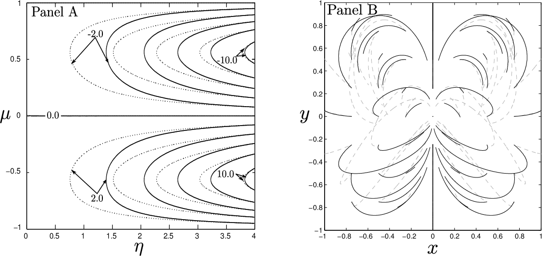
We compare in Figure 12 the semi-analytic solution with the new solution (subscript “num” denotes the new numerical solution). We also show in this figure that the new numerical solution is not a separable solution. Panel A reveals that varies significantly, while a result of rescaling would give a constant ratio. Panel B, which shows with a fixed value, illustrates that the new numerical solution descends faster to zero than the semi-analytic solution when goes to (or equivalently, when goes to ). It also tells the impossibility of separating variables: they indicate that has different patterns if we assign to different values and plot against . Panel C shows the non-separability in another aspect: we present the variation of , where is a constant value and is value of the at the boundary. Clearly is not a constant, which is in contrast with separability.
Nevertheless, as was found in our extensive numerical explorations using both FDM and FEM schemes, when we prescribe the boundary condition (40) (with as an example) for nonlinear PDE (36), we would obtain via iterations a numerical solution which is definitely different from the separable semi-analytic nonlinear solution. At least, this can be done in a sequence of nonlinear solution pairs with the same boundary conditions. As an example of illustration, we present in Panel A of Figure 11 a comparison between a pair of semi-analytic results with , (i.e. ), and its corresponding numerical nonlinear solution determined by the above procedure. Meanwhile in Panel B of Figure 11, we compare magnetic field lines of force generated by two different solutions in the pair. For each type of solutions, we plot 49 magnetic field lines of force starting from 49 evenly spaced points lying on the plane with and (these are Cartesian coordinates), as was done in panel (b) of figure 3 by Low & Lou (1990). The differences are patently clear. The existence of multiple nonlinear solutions prompt us to further explore the steady MHD problem with possible multiple nonlinear solutions described in this paper.
We highlight the following statements regarding the development and tests of numerical extrapolation MHD codes over decades to construct various configurations of solar/stellar and astrophysical disk coronal magnetic fields. For example in the solar case, it is highly desirable for solar physicists to infer coronal magnetic fields based on the measurements of solar photospheric magnetic fields (e.g. Low & Lou, 1990, and references therein). Realizing the real possibility of multiple (currently at least two by our MHD model analysis) nonlinear solutions with the exactly same boundary conditions, the numerical code development for extrapolating magnetic field configurations from specified or measured surface conditions would face considerable challenges and should proceed with extreme cares. Essentially, this dilemma would involve computation selection effects of numerical solutions and nature selection effects of physical solutions. Two key questions are then: How do we know that our extrapolation MHD codes are reliable through tests against known solutions? What are the paths of choosing separate numerical solutions? In a sense, we need to know and determine all multiple solutions for the same boundary conditions if there are indeed more than two. Otherwise, we would be highly uncertain about the convergence of our numerical solutions as settled by our extrapolation MHD codes. One conceivable yet unfavorable situation would be the undesirable artificial exclusion of possible numerical solutions because of the implementation of a particular numerical scheme under certain constraints. Even if all numerical solutions with the same boundary conditions are know and available, we would then need additional physical information and/or requirements to remove such degeneracy of multiple nonlinear solutions. Or, they are all realizable in nature. We would like to know their stabilities as well as their mutual or independent evolution. This appears to be a new dimension/perspective for this research field involving nonlinear degeneracy.
One implication of these findings for multiple (i.e. non-unique) nonlinear solutions is that they might cause “peculiar things” that may happen in simulation tests for numerical MHD codes to extrapolate solar/stellar and astrophysical disk coronal magnetic fields from the photosphere, especially those likely involving aspects of the “ill-posed” problems as emphasized by Low & Lou (1990).
For a clearer presentation of this problem and further discussion, we indicate below four common “diagnostics” (Amari et al., 2006, e.g.) of our numerical nonlinear solutions, one of which is fairly similar to equation (23) in subsection 5.2.2. First, we state the mathematical definitions of those “diagnostic functions”. The correlation of vector magnetic fields:
| (41) |
the Cauchy-Schwartz correlation of two vector magnetic fields:
| (42) |
the normalized error of a vector magnetic field:
| (43) |
and the mean error of a vector magnetic field:
| (44) |
In the foregoing four expressions, is the differential volume element and is the spatial volume for integration. Clearly, if the two vector fields are identical everywhere inside the spatial volume for integration, we should have and . In other words, the amounts by which the correlation functions ( and ) deviate from and/or the error functions ( and ) deviate from indicate the extent for which deviates from .

We take the spatial integration volume in eqs. (41) to (44) to be a spherical shell whose inner radius is and outer radius is which is adjustable. In Figure 13, we illustrate these four “diagnostic functions” as functions of . One can see clearly from Figure 13 that the correlation functions, especially the Cauchy-Schwartz correlation, drops significantly below as the integration volume becomes larger, which reveals that the novel numerical solutions deviate from the corresponding semi-analytic ones more severely in a larger spatial volume. The increase of the two error functions for vector magnetic fields shown in Panel B reveals a similar trend.
Calculations of these four “diagnostic functions” are frequently performed in the literature concerning the numerical extrapolation scheme of force-free magnetic fields, e.g. Valori et al. (2007), Hu & Dasgupta (2008) and Li et al. (2009). Although the verification of numerical extrapolation algorithms seem to have good consistency with the results of Low & Lou (1990), our numerical calculations here, taken with respect to the novel numerical solution and the semi-analytic solution, suggest that significant deviations may also occur due to the nonlinearity of the force-free equation. Possibly those discussions could be responsible for “not-so-good” results of extrapolation tests [e.g. He & Wang (2008) and Liu et al. (2011)], aiming at reproducing separable semi-analytic results in Low & Lou (1990).
Appendix C Derivation of the key scalar nonlinear elliptical PDE
In this Appendix C, we summarize the major steps that lead to the key scalar nonlinear elliptical PDE (5) (Throumoulopoulos & Tasso, 2001, see also).
In nonlinear PDE system (2), a divergence-free vector field of axisymmetry can be generally expressed in terms of a toroidal component and a poloidal component (Chandrasekhar, 1956, e.g.) in the form of
| (45) |
where and are two scalar functions of and , and in the spherical polar coordinates . An axisymmetric scalar field with the symmetry axis along always satisfies the condition of .
By projecting the Ohm’s law of infinite conductivity, i.e. in the azimuthal direction and assuming axisymmetry, we have
| (46) |
after straightforward manipulations of vector identities. As the only non-zero component of is the component, we simply have from the last factor in condition (46) above. Similarly, we also derive by projecting the Ohm’s law of infinite conductivity along the magnetic field direction. We readily have by integrating and it also follows similarly that .
Another useful relation can be derived by projecting the Ohm’s law of infinite conductivity along , yielding
| (47) |
after straightforward manipulations. This gives rise to the second line in equation (3) by simply inserting the two relations and derived above.
Before more integral relations, we invoke below two useful equations. The first one is the familiar vector identity
| (48) |
The second one involves the axisymmetric function ,
| (49) |
where .
Two identities (48) and (49) are inserted into the second line of (1), i.e. the momentum equation. Using equations (2), the left-hand side (LHS) of equation (48) can be further expanded in the form of
| (50) |
The specific Lorentz force term can also be expanded in the form of
| (51) |
We first project the momentum equation along the azimuthal direction to obtain
| (52) |
where equation (47) is used. We then use the definition of in the third line of equation (3) and , which naturally leads to and hence turns out to be another free functional in our MHD formalism.
The momentum equation along the direction yields
| (53) |
where because is a full function of and is the gravitational potential. We now impose the condition of incompressibility leading to and thus . Equation (53) can be cast into the form of
| (54) |
where we have invoked the last two lines in equations (3) to eliminate . The following equation is also applied in deriving equation (54), viz.
| (55) |
where , and are all full functionals of . If we define the sum of all terms within the curly brace of equation (54) to be , we thus infer similar to what we did for and , where the definition of variable is consistent with the first line of equation (3).
The scalar nonlinear elliptical PDE can be derived by projecting the momentum equation along direction. It is then straightforward yet tedious to obtain
| (56) |
We simplify PDE (56) by substituting the definition of [i.e. the first line of equation (3)] and the definition of poloidal Alfvénic Mach number via (see subsection 3). Straightforward manipulations then yield
| (57) |
We then utilize transformation (4) to finally arrive at scalar nonlinear elliptical PDE (5).
Appendix D Functional analysis for FEM software
Unlike equation (15),
FreeFem++ uses one or two testing
variation testers in the FEM space.
Therefore, it gives a functional analysis problem, where
the “zero point” of the following functional
instead of a “minimum point” needs to be found:
| (58) |
Here is the variation tester. In order to find the zero point, another tester should be introduced to calculate :
| (59) |
Since the PDE is not linear, we shall expect a Newton iteration scheme for the final solution to the non-linear problem. The computational steps during each iteration are taken as follows:
- 1.
Calculate with current , presented as a vector.
- 2.
Calculate , presented as a matrix.
- 3.
Update the value of by .
The detailed code and conditions may vary from a specific problem to another, and from a user to another, but the essentials remain the same as outlined above.