Coaxing Cosmic 21 cm Fluctuations from the Polarized Sky using -mode Analysis
Abstract
In this paper we continue to develop the -mode formalism, a technique for efficient and optimal analysis of wide-field transit radio telescopes, targeted at cosmology. We extend this formalism to give an accurate treatment of the polarised sky, fully accounting for the effects of polarisation leakage and cross-polarisation. We use the geometry of the measured set of visibilities to project down to pure temperature modes on the sky, serving as a significant compression, and an effective first filter of polarised contaminants. As in our previous work, we use the -mode formalism with the Karhunen-Loève transform to give a highly efficient method for foreground cleaning, and demonstrate its success in cleaning realistic polarised skies observed with an instrument suffering from substantial off axis polarisation leakage. We develop an optimal quadratic estimator in the -mode formalism, which can be efficiently calculated using a Monte-Carlo technique. This is used to assess the implications of foreground removal for power spectrum constraints where we find that our method can clean foregrounds well below the foreground wedge, rendering only scales inaccessible. As this approach assumes perfect knowledge of the telescope, we perform a conservative test of how essential this is by simulating and analysing datasets with deviations about our assumed telescope. Assuming no other techniques to mitigate bias are applied, we find we recover unbiased power spectra when the per-feed beam width to be measured to , and amplifier gains to be known to within each minute. Finally, as an example application, we extend our forecasts to a wideband cosmological observation and consider the implications for probing dark energy, finding a pathfinder-scale medium-sized cylinder telescope improves the DETF Figure of Merit by around over Planck and Stage II experiments alone.
I Introduction
Recent years have seen a surge in excitement at the promise of radio cosmology. By using low frequency observations of the line we can survey the distribution of neutral hydrogen throughout large volumes of the Universe. Radio interferometers provide an efficient, and cost effective method for doing this.
This transformation of radio interferometers into survey instruments has been driven by recent technological advances, particularly in the cheap low-noise amplifiers required for mobile phones, and the constant progress of Moore’s law making large, high bandwidth correlators economical. By correlating a large number of low cost feeds in a compact area we can produce a telescope ideally suited for wide-field surveys.
There are three main epochs we can observe: low redshift (), where we observe the large scale emission from unresolved galaxies, a technique termed intensity mapping [1, 2]; the Epoch of Reionisation (–) where the neutral IGM is eaten away by the first ionising sources [3]; and perhaps even the primordial structure in the dark ages (), though observations at these very low frequencies () will be extremely challenging [4]. These eras are of huge cosmological importance, a fact reflected in the large number of current and planned experiments targeting observations, with GMRT [5], HERA [6], LOFAR [7], MWA [8], MITEoR [9] and PAPER [10] targeting the Epoch of Reionisation and BAOBAB [11], BAORadio [12], BINGO [13], CHIME [14], EMBRACE/EMMA [15], Ooty [16], Parkes [17] and Tianlai [18] aiming at the low redshift intensity mapping era.
In this paper we will focus on the low redshift, intensity mapping epoch, though most of the results and techniques we describe apply equally well at higher redshift. Observations at these low redshifts target the same science as spectroscopic galaxy redshift surveys such as [19, 20]: measuring Baryon Acoustic Oscillations and through them probing the expansion history of the Universe [21, 22, 23]. However, they are very complimentary, with radio observations probing a larger volume at higher redshift, with a completely different set of systematics.
To make effective use of this new generation of radio interferometers, we must develop new methods of interpreting and analysing their data. Progress has accelerated in recent years with many developments [24, 25, 26, 27, 28, 29, 30, 31].
In a previous paper [32] we developed a new techique for the analysis of data from these experiments called the -mode formalism. This method departs from the usual interferometric analysis—making no flat-sky or small field approximations—at the expense of being limited to transit telescopes for which it is an exact treatment. It also brings computational advantages by allowing us to break the data into uncorrelated -modes, making it feasible to treat the full statistics of the data. This opens up the possibility of performing optimal map making, foreground subtraction, and power spectrum estimation, which would be extremely difficult otherwise.
Perhaps the foremost challenge facing cosmology is the presence of bright astrophysical radio sources at frequencies below which are around six orders of magnitude brighter than the signal. This emission comes mainly from synchrotron radiation, which is spectrally smooth, and in principle this allows it to be separated from the as it is described by a small number of modes [33] and these can simply be removed. The remaining modes, which have significant spectral structure are assumed to be free of contamination. Unfortunately, this picture is complicated by the realities of radio observation:
- •
Frequency dependent beams lead to mixing of angular structure into spectral structure which contaminates the foreground clean modes [34]. This problem, known as mode mixing, means that looking at only the frequency direction of our data is insufficient to separate these two signals.
- •
Synchrotron emission from our galaxy is highly polarised, and though the totally intensity is spectrally smooth, Faraday rotation by the magnetic interstellar medium means that the polarised emission is not. Unfortunately, the complicated polarisation response of real telescopes irreversibly mixes some fraction of the polarised sky, introducing significant frequency fluctuations [35]. As the emission comes from a range of Faraday depths, we cannot simply de-rotate the emission.
Fundamentally there are still the same number of large foreground modes, mode mixing only makes them harder to identify. In [32] we developed a foreground removal technique based on the Karhunen-Loève (KL) transform. This uses the full covariance statistics of the contaminating foregrounds to find an optimal separation from the signal, fully accounting for this mode mixing effect. However, the technique presented there was limited in two important ways: no attempt was made to address the problem of polarised foregrounds; and it assumed that we have full knowledge of the properties of our instrument, including the full polarised response of the primary beam, and any per-feed amplitude gains and phase shifts introduced in the receiver system. In this paper we continue to develop both the -mode formalism and KL transform for foreground cleaning, with particular emphasis on investigating these two limitations.
We start by extending the -mode formalism to give a full treatment of polarisation (Section II), and discuss how the unpolarised approach of [32] is a limiting case (Section III)). The example telescope we use throughout is described in Section IV, and its harmonic space sensitivity is examined in Section V. Next we take a careful look at the geometry of the measured -modes (Section VI), leading us to a technique which both efficiently compresses the data and effectively removes polarised contamination. We give an overview of the Karhunen-Loève scheme for foreground removal in Section VII, and demonstrate its effectiveness on simulated polarised skies. In Section VIII we construct an optimal power spectrum estimator in the -mode formalism, which we use to study the performance of our foreground filter (Section IX). In Section X we use this estimator to show how instrumental uncertainties give rise to power spectrum biases. Finally we forecast the performance of our example telescope at measuring the expansion history of the Universe and constraining the nature of dark energy (Section XI).
II Polarised Transit Telescope Analysis
In this section we develop a fully polarised version of the -mode formalism, a new method for analysing transit interferometers that was first introduced in a previous paper [32]. That treatment encapsulates all the essential ideas but avoids the added complexity of tracking the polarisation, and is a useful introduction to the full treatment given here. Polarised descriptions of full-sky interferometry have been given elsewhere (notably [36, 37]), but here we develop the transit telescope limit.
Any transit telescope can be viewed as a collection of feeds, fixed relative to the ground frame. Each feed, measures a combination of the electric field coming from various directions on the sky. In order to accurately treat the polarisation when the response varies over the sky, we need to be able to keep track of the contribution from each direction to the electric field at a point. In order to do this we define as the electric field density in a frequency interval and solid angle by
| (1) |
With this definition the Poynting flux is conveniently written as
| (2) |
Radio emission from the sky is generally incoherent and so we can write the correlations of explicitly in terms of the Stokes parameters
| (3) |
where the indices are over basis vectors transverse to the line of sight. As in the unpolarised case we are more interested in the brightness temperature on the sky, and so we have written Equation 3 to make that explicit (thus , , and are polarisation brightness temperatures). The polarisation tensors are related to the Pauli matrices (in an orthonormal basis), specifically
| (4) |
The standard basis to use in spherical geometry are the polar and azimuthal directions, and , as these allow spin spherical harmonics to be used straightforwardly to decompose the polarisation field.
Any feed on the telescope measures a weighted combination of the electric field coming from each direction on the sky. In particular we need to keep track of the antenna’s sensitivity to the orientation of the incoming electric field. We’ll write the measured signal at the -th feed, as which is given by
| (5) |
and is directly proportional to the voltage induced in the circuit. Here, and onwards, we will implicitly sum over the polarisation index . The antenna reception pattern is a vector quantity describing the electric field response in a given direction. The response , the effective antenna length (choosing them equal would make be the antenna voltage). We normalise such that the normalised antenna power pattern ensuring the solid angle of the beam is
| (6) |
In Equation 5 we have also included an exponential factor which gives the phase relative to an arbitrary reference point. As both this, and the antenna orientation change with the Earth’s rotation relative to the sky, we write them as functions of , the rotation angle.
The fundamental quantity in radio-interferometry is the cross correlation between two feeds, the visibility . Using Equations 5 and 3 we can write down exactly what a visibility measures, explicitly keeping track of the different sky polarisations to give
| (7) |
where the beam transfer functions encode all the information about the optics and geometry of the instrument. They are given by
| (8) |
where . The measured visibilities are corrupted by noise, which we include as an additional term . In this work we will assume that the noise from different antennas, and frequencies are uncorrelated (we discuss the statistics in more detail in Appendix A).
We normalise our visibilities so that they are the correlated antenna temperature in the noiseless limit (in particular the auto-correlation is the antenna temperature). The factor of two in the definition of the transfer function ensures that for an unpolarised sky with uniform brightness , the measured autocorrelation . Note that in Equation 7 and onwards the symbol denotes two different quantities, the visibility and the Stokes V sky field . The distinction will be clear from the context.
The above Equations 7 and 8 are completely exact. The general approach to interferometric analysis is to approximate the above to a 2D Fourier transform, which is valid for small fields of view. For wide-field observations we can attempt to relax this with techniques such as mosaicing [38] and -projection [39] though this quickly becomes complicated. In our case we are interested in a specific class of transit interferometers intended for surveys. However, as these instruments are extremely wide-field, this approach is limiting. Instead we will try a different route, restricting our domain to transit telescopes, but otherwise attempting to keep the analysis exact.
To continue, we decompose into spherical harmonics, as they are a natural way of representing fluctuations on the sky. As polarisation is not a scalar field we must expand and in spin-2 harmonics (the Stokes field transforms as a scalar). This yields
| (9) | ||||
| (10) | ||||
| (11) | ||||
| (12) |
The polarised beam transfer matrices also transform as spin fields, and so we decompose them in the same way, with
| (13) | ||||
| (14) | ||||
| (15) | ||||
| (16) |
Note that we have decomposed with the complex conjugates of the spin-harmonics. This allows us to use the orthogonality of the (spin) spherical harmonics to rewrite the visibility equation Equation 7 as
| (17) |
Though this has completely transformed the problem into harmonic space, it will be more convenient if we change into the conventional and mode decomposition as they are real scalar fields [40]. This can be done by making the standard substitutions
| (18) | ||||
| (19) |
as well as the corresponding changes for the beam matrices
| (20) | ||||
| (21) |
leaving the visibility as
| (22) |
In the above the harmonic coefficients are now all the transforms of real scalar fields (the are the complex conjugates of the spherical harmonic coefficients).
Given the periodicity of the system in , Fourier transforming Equation 22 is an obvious next step
| (23) |
We call these Fourier coefficients, -modes, and they will become the key quantity in our analysis. As the visibility is a complex timestream, the positive and negative ’s are independent measurements.
As the dependence simply rotates the functions about the polar axis the transfer function is trivially . The integral over the exponential factors generates the Kroenecker delta and removes the summation over entirely, and we can write the -modes as
| (24) |
Though slightly hidden, this a property of the convolution theorem. For a transit telescope the visibility timestream is an azimuthal convolution of the beam and sky. This means its Fourier conjugate, the -modes, are products of the individual Fourier modes (with a remaining summation over the index). This equation fully describes how the measured visibilities are related to the polarised sky that we are observing.
It is worth thinking about what we are measuring. The visibility we see is a complex time series, which roughly corresponds to the signal from the sky modulated by a complex Fourier mode. In our case the time variable is , the Earth’s rotation. Taking the Fourier transform of a visibility splits the time series into right and left moving waves (positive and negative respectively). A correlated beam pointing south of the north pole only produces modes moving in one direction (as the beam on the sky is a Fourier mode), however pointing the same beam beyond the north pole (that is north of it as defined in the ground frame), produces the other modes as the Fourier mode on the sky moves in the opposite direction with respect to the Earth rotation. One important consequence of this is that if we use the freedom to choose the order of the our feed pairs such that the baseline vectors point towards the east, positive -modes are produced below the pole, and negative -modes come from above. If the primary beam does not extend over the pole only positive ’s are produced, though a small amount of negative ’s are seen because of the effect of the primary beam.
In fact, whilst the positive and negative -modes may be independent measurements they are still observations of the same sky — for a real field and thus both and measure the same harmonics on the sky. It will be useful to change our notation to make this fact transparent.
Let us separate out the positive and negative parts by defining
| (25) | ||||||
| (26) |
which is valid for . Additionally to prevent double counting the measurement we need to set . For brevity of notation, we will introduce a label which indexes both the positive and negative parts of all included feed pairs , such that any particular specifies exactly the values of (exactly how is packed is unimportant). This gives the final form of the -mode visibility equation that we use as the basis of this work,
| (27) |
As in [32] we can write this equation in an explicit matrix form which will allow us to simplify the notation. The beam transfer matrices above can be written in an explicit matrix notation
| (28) |
where the row index labels all baseline () and frequency combinations (), whereas the column index is over all multipole () and frequencies (). Similarly we can define vectors for the visibilities and harmonic coefficients
| (29) |
To keep track of the different polarisation states we define the block matrix and vector
| (30) |
such that
| (31) |
This is the essence of the -mode formalism: a simple, linear matrix relation that exactly describes the whole measurement process for a transit interferometer. As we will discuss in Section V both the number of -modes and the dimensionality of the matrices is bounded by the physical size of the instrument. This means that we can easily apply all the standard tools of statistical signal processing without even remembering that we’re dealing with an interferometer. In the following sections we do this with gusto.
Despite this being an interferometry paper, the -plane has not been mentioned at all so far. Though it is prevalent in many interferometric applications, as both an extremely useful aid for physical understanding and for computational efficiency (by virtue of the FFT), the -mode formalism does not make use of it. Eschewing the -plane is part of its power, helping it to work trivially for wide-field analysis, and focusing us on only the measured degrees of freedom. However, it comes at the cost of making it difficult to have concrete physical interpretations of the process.
III Unpolarised Limit
In [32] we developed an unpolarised formalism because it gives a simpler problem to analyse, both conceptually and computationally. However, under certain assumptions it is directly equivalent to the full polarised case.
For a telescope with dual polarised antennas, let us suppose that we can engineer our telescope optics such that the field patterns of the two feeds (labelled and ) obey two constraints. First, that their normalised power patterns are equal everywhere
| (32) |
and second that their polarisation orientations are orthogonal all over the sky
| (33) |
Under these constraints there is only one relevant linear combination of the four , , and visibilities that is sensitive to the total intensity, the average of the and visibilities
| (34) | ||||
Because of the properties of the polarisation matrices, this is not sensitive to the different polarisation modes , and , whilst all the orthogonal combinations are insensitive to the total intensity .
In this limit, the combination is equivalent to the unpolarised formalism given in [32], if we relabel the noise terms such that . Provided the noise terms are uncorrelated this reduces the power spectrum down by a factor of two — that is the unpolarised system temperature is .
IV Cylinder Telescopes
Cylinder telescopes are interferometric arrays consisting of one or more parabolic cylindrical reflectors. They have a long history in radio astronomy, with well known facilities like the Molongo Synthesis Telescope [41], and the Ooty Radio Telescope [42]. Though advances in amplifier technology meant they steadily lost favour to dish-based interferometers, interest in them has recently been revived. Reasons are twofold: the development of cheap, room temperature, low noise amplifiers has dramatically improved sensitivity; and intensity mapping has provided an application for which they are ideally suited.
Intensity mapping requires a large collecting area in a compact region to achieve high brightness sensitivity, which cylinders can provided cheaply. Additionally cylinder telescopes are a cost effective way of surveying large amounts of sky at high speed [43]. And whilst arrays of dipoles provided a bigger instantaneous field of view, the large number of elements required at a fixed angular resolution makes the receiver and correlation hardware increasingly expensive.
Each cylinder has a parabolic cross section such that they focus only in one direction. In the layout we assume (see Figure 1), this gives a long and and thin beam on the sky, extending nearly from horizon to horizon in the North-South direction but which is only around 2 degrees wide East-West. Feeds are spaced along the axis of each cylinder — when correlated these provide resolution in the N-S direction. As the telescope operates as a transit telescope this means that the entire visible sky is observed once per sidereal day.
In this paper we illustrate the -mode formalism using a medium sized cylinder telescope, similar to the CHIME Pathfinder. Table 1 lists the parameters of this example instrument.
| Parameters | Value |
|---|---|
| Number of cylinders | 2 |
| Cylinder width [m] | 20 |
| Feeds per cylinder | 64 (dual-pol) |
| Feed spacing [m] | 0.3 |
| [K] | 50 |
| Bandwidth [MHz] | – |
| Channel width [MHz] | 2.5 |
| Number of Channels | 160 (in groups of 40) |
| Telescope Latitude |
IV.1 Beam model
In the -mode formalism knowledge of the primary beams of our instrument is crucial. In our model we assume an arrangement such that at each location there are two perpendicular dipoles: the feed where the dipole is aligned across the cylinder (pointing East), and feed where the dipole is aligned along the axis (pointing North). In both cases the feeds hang below a conducting ground plane which stops the beam spilling above the cylinder (which is assumed to have an f-ratio of ).
Solving for the beam on the sky for a feed placed in a parabolic cylinder is a complex problem (for one approach see [44, 45]). Crudely the cylinder acts in two ways: in the parabolic direction it focuses the antenna beam to a diffraction limited beam on the sky; in the orthogonal direction it acts like a mirror, inverting the antenna beam. Rather than try to accurately solve for the beam, we try to capture these two effects. We will break the model down into the product of two 1D functions: a function for the E-W direction, calculated by illuminating the cylinder with the dipole beam, and solving for the diffraction in the Fraunhofer limit; and a N-S function which is just the reflected feed amplitude in the N-S direction. We will also model the polarisation direction as being the same as that of an unfocused dipole (in spherical co-ordinates, for a dipole along the polar axis, the polarisation direction is ).
First we model the beam amplitude for the unfocused dipole in the E-plane and H-plane as taking the form
| (35) |
where is the full width at half-power of the beam. For a horizontal dipole mounted a distance over a conducting ground plane (see [46, section 4.7]), we can exactly calculate the widths in the H-plane () and E-plane (). We use these value for our fiducial beam model, though we will vary them later in this paper.
In the E-W direction we are solving the Frauhofer diffraction problem of a cylinder feed illuminating an aperture of a finite width. This has the solution
| (36) |
where we have used the fact that for a cylinder with an f-ratio of a ray striking a distance from the cylinder centre reflects by an angle where W is the cylinder width.
Putting these components together, our overall beam model can be written as the product of three functions. For the feed
| (37) |
and for the feed
| (38) |
where the vectors is a unit vector transverse to the cylinder, pointing East, and is along the cylinder, pointing North. The function gives the unit vector polarisation direction on the sky for a dipole in direction
| (39) |
In Figure 2 we illustrate the on-sky beam for this our example telescope. We plot the response of an ‘instrumental Stokes I’, constructed from the combination of polarisation, to Stokes I and polarisated emission on the sky. The reponse to Stokes I on the sky is given by
| (40) |
As a measure of the response to polarised radiation we use
| (41) |
For a beam with no polarisation leakage, this response is zero. Though our example has no leakage on-axis, Figure 2 clearly shows that there is significant pickup of polarisation away from the beam centre.

V Sensitivity in Harmonic Space
The geometry of an interferometer on the ground determines its angular sensitivity on the sky, with the total size of the optical system determining the smallest scales that can be measured. This limits the number of harmonic modes on the sky that we are able to measure, reducing Equation 27 to finite sums.
The set of spherical harmonics that a given baseline is sensitive to can be found by expanding a plane wave on the sky
| (42) |
where the part in square brackets is the coefficient in a spherical harmonic expansion of the plane wave. The amplitude of a spherical harmonic function can be conveniently written in terms of integrals of Bessel functions [47, section 5.4]. For large we find
| (43) |
where we have used the approximation that . Combining this with Equation 42 shows that the magnitude of the spherical harmonic coefficients of a plane wave are
| (44) |
In particular this shows that the coefficients are effectively bounded in a triangle by and because of the exponential decay of the Bessel functions for large order.
The highest frequency fourier mode measured on a sky by an individual baseline comes from the maximum distance between illuminated areas on the correlated antennas (this is the largest distance from the origin in the -plane). Following through from Equation 44, we expect the range of measureable modes to be and , where is the largest distance assoicated with baselines and the largest in the E-W direction.
Let us consider our cylinder (see Figure 1). A feed on the cylinder effectively illuminates the whole width of the cylinder, but a very short distance along its axis. This makes the largest E-W distance of all feed pairs , and the largest N-S distance . In terms of spherical harmonics coefficients on the sky, we are limited to
| (45) | ||||
| (46) |
Though this result is correct for a cylinder telescope, for an interferometer with a compact field of view, pointing away from the celestial equator, it needs modifying. As before the resolution in the E-W direction is determined by the maximum distance , however, if the primary beam does not cross the equator this resolution corresponds to a larger fraction of the circle of constant declination at that point. As the -mode corresponds to the Fourier mode in the azimuthal direction, this means that the limit on is in fact , where is the declination of the point in the primary beam closest to the celestial equator.
To look at the sensitivity of the telescope in more detail we can calculate the Fisher matrix of the coefficients (we discuss the interpretation of Fisher matrices in detail in Section VIII). For Gaussian noise the likelihood function for the ’s is
| (47) |
From this we can calculate the Fisher matrix for a particular
| (48) |
We expect that in general this matrix will be singular and hence we cannot find the covariance matrix of the coefficients by finding . One obvious source of this is that the interferometer does not see the whole sky — anything declination less than is below the horizon — and this manifests itself as correlated combinations of ’s that we cannot separate. Additionally the angular resolution falls off towards the horizon meaning that we do not have uniform sensitivity across the sky.
This consequence of this is obvious from simply counting the degrees of freedom involved. For the example telescope, there are 762 unique baselines each of which gives a noisy complex measurement of the sky. However, we are sensitive up to for each polarisation, giving complex degrees of freedom on the sky, so there must be some combinations about which we have no information.
As in general we cannot determine the covariance matrix of the , we will use the Fisher matrix itself to describe the sensitivity. In Figure 3 we show the diagonal elements of the Fisher matrix at each for the example telescope, this gives an illustration of the amount of information we have about any spherical harmonic mode.

VI SVD projection
For cosmology we are only interested in deriving real properties of the unpolarised sky. As we shall see this is usually of much lower dimension than the space of measurements made by an interferometer, leaving a large number of redundant degrees of freedom which are just filled by the instrumental noise. Eliminating these would allow us to significantly compress the data space, without losing useful information. In Figure 4 we illustrate the geometry of the measured visibilities. The matrix wholly describes the mapping between the sky and the measured visibilities, and understanding its structure is the key to isolating the important degrees of freedom.
To start with let us concentrate on how to reduce to only the degrees of freedom on the sky (ignoring their polarisations for now). The matrix tells us how a subspace of the spherical harmonics map into a subspace in visibility space . This visibility subspace (shown by the plane in the Figure 4), is termed the image of . The subspace of visibilities orthogonal to the image, is called the cokernel. The cokernel has no mapping to the sky, and so measuring this subspace yields no useful information. By projecting our data onto the image, we remove the cokernel and compress our data by retaining only the relevant degrees of freedom. In Figure 4 this corresponds to projecting onto the plane, eliminating the perpendicular dimensions.
The number of retained degrees of freedom is given by the dimensionality of the image — that is, the rank of — and cannot exceed the number of measured modes on the sky. For a single frequency and , the rank is guaranteed to be less than the total number of spherical harmonics required to describe the polarised sky, that is . However, in the case of incomplete sky coverage, we cannot measure all spherical harmonic modes independently, and this coupling means that the rank is likely to be reduced to around , where is the fraction of sky observed.
These numbers depend only on the physical size of the telescope, and not details of the feed distribution. For compact interferometers with little redundancy, the number of feed pairs rapidly exceeds the rank of the matrix, and so projecting onto the image gives a large computational saving.
To find the image of we can use the Singular Value Decomposition (SVD). However, first we will pre-whiten the visibilities with respect to the instrumental noise. This transforms it to be uncorrelated with unit variance and can be done by multiplying them with , a matrix such that . As is positive definite this factorisation always exists and can be found by Cholesky factorisation or eigendecomposition. This leaves Equation 31 as
| (49) |
We then take the SVD of the whitened beam transfer matrix
| (50) |
The matrix defines the image and cokernel, given by columns of corresponding to non-zero and zero singular values respectively. In practice many singular values are numerically small but not precisely zero, giving modes which are either non-zero because of numerical precision, or simply carry a very small but non-zero amount of information about the sky. In this case we separate the image and cokernel using a numerical threshold. We partition the columns of the matrix into two matrices and which give the image and cokernel respectively. To compress our data we simply filter with the matrix to give .
While this filtering can yield a large compression, we should note that it preserves all the information about the sky. However, the cosmological signal we are interested in is purely unpolarised and requires only modes per frequency and to describe it. This suggests that we should be able to improve our compression by around another factor of four.
As a first attempt we might consider projecting onto the image of , the total intensity transfer matrix, rather than the full . In Figure 4 this would correspond to projecting straight onto the vector, rather than just the plane.
Unfortunately as illustrated in Figure 4, the image of the total intensity need not be orthogonal to the subspace containing the polarised image. This is a manifestation of polarisation leakage. In this case by doing this we lose the ability to differentiate between polarised and unpolarised signals from the sky, resulting in catastrophic leakage of polarised foregrounds.
A resolution to this problem is to project not onto the image of but to perform another projection, this time onto the polarisation cokernel. In Figure 4 this is equivalent to projecting onto the vector . By doing this we ensure that there is no leakage of the polarised sky into our compressed data, at the expense of throwing away information about the total intensity signal that lies in the overlap between the two spaces.
To project out the polarised signal, we first construct the polarisation transfer matrix
| (51) |
then we use this to isolate the polarisation cokernel in the sky compressed basis by performing another SVD
| (52) |
As before we separate into the image and cokernel of this matrix, by dividing up into and respectively. As before the separation onto the two spaces is not exact, but done through a numerical threshold. By projecting our dataspace onto the cokernel we achieve this final compression.
Overall we have applied three transformations to our data:
- •
Whiten the instrumental noise by applying
- •
Project onto the sky subspace by using
- •
Project out the polarised sky using
Combined these define a new basis in which to consider our data. One which strives to preserve as much of the relevant information as possible, whilst vastly reducing the number of degrees of freedom we must consider. We define our filtered visibility data as
| (53) |
We can write a modified version of the measurement equation (31) which relates this to the sky signal
| (54) |
where we have defined
| (55) | ||||
| (56) |
As the columns of and are orthonormal, the instrumental noise still has the identity covariance . In Figure 5 we show the singular values of the new mapping matrix , clearly illustrating that we are only sensitive to a small number of modes on the sky.
In order to visualise our data we will want to make maps from our filtered dataset. For Gaussian distributed instrumental noise it is straightforward to make maximum likelihood maps of the sky as discussed in [32]. As we have whitened the instrumental noise, our data has a likelihood function
| (57) |
and thus we can solve for the maximum-likelihood solution using the Moore-Penrose pseudo-inverse, giving our best estimate of the spherical harmonics simply as
| (58) |
As in [32], to make a full map of the sky, we simply use this estimator on a per- and per frequency basis and collate the estimates. We can then perform an inverse Spherical Harmonic Transform to produce sky maps at each frequency. As we have projected onto the polarisation cokernel, the data does not contain any information about the polarised sky. Combined with the minimum power property of the Moore-Penrose pseudo inverse this means that the polarised spherical harmonics will be zero.

VII Foreground Removal with the Karhunen-Loève Transform
The foremost challenge for any intensity mapping experiment is separating the cosmological signal from astrophysical contaminants which are around – times larger. The primary sources are the diffuse synchrotron emission from our own galaxy and emission from extra-galactic point sources [48]. All significant foregrounds are expected to be spectrally smooth [33], however, the signal decorrelates quickly as each frequency corresponds to a different spatial slice. This gives an opportunity to separate the two.
Conceptually foreground removal is simple—we just remove the smooth frequency component from our observations. Unfortunately the reality is far from straightforward. The large dynamic range between the amplitude of the foregrounds and the signal makes several effects extremely problematic.
- Mode mixing
-
In a real experiment the shape of the beam on the sky will vary with the observed frequency, driven by the optical effects of using a fixed physical aperture or feed spacing. Even if the angular fluctuations on the sky were frequency independent as we scan through in frequency the beam structure changes, and this introduces variations of our measurements with frequency.
- Model uncertainties
-
Astrophysical foregrounds are poorly constrained at the small angular and frequency scales that will be probed by upcoming intensity mapping experiments. Whilst there exist theoretical and phenomenological models of this regime, a successful foreground removal method should be robust to uncertainties in the foreground statistics. Though most effort has focused on the uncertainties in the two-point correlations, we must also ensure that higher order moments do not impair our analysis.
Given these complications, we would prefer a foreground removal method to be conservative, throwing away potentially useful information in order to be robust to them. It is better to be cautiously correct than precisely wrong.
Accepting that we may prefer to lose information about the signal in order to be unbiased by residual foregrounds, we would still like to perform the best job we can, requiring that we are
- Statistically Optimal
-
Whatever space the foregrounds are removed in we must be able to keep track of the statistics of both the instrumental noise, and the foreground residuals in order to be able to optimally perform subsequent stages, notably power spectrum estimation.
This latter point is especially pertinent for any technique that operates directly in map space. It is not only difficult to express the pixel-pixel correlations caused by the measurement process (especially with noise), but similarly difficult to project these back after any foreground cleaning has been performed.
In a previous paper [32] we developed a foreground removal technique that addresses these three issues. It does this by explicitly taking into account the statistics of both the signal and foregrounds in the basis that they are measured. In this Section we give an overview of this method in the context of the polarised analysis presented here.
VII.1 Stationary Statistics
Understanding the statistics of our measured data is essential ingredient in all but the most basic analysis if we make best use of the data. For intensity mapping experiments, our data has three components: the signal which we are trying to extract, the foregrounds, and instrumental noise. The statistics of instrumental noise live in the visibility space, the basis of our measurements. However the other components are naturally represented on the sky, and must be projected into this space using Equation 58.
In this work we treat the sky as a statistically isotropic field with a two-point function
| (59) |
which we write in matrix form as defined as
| (60) |
This quantity can be projected into the SVD basis for a given using the transfer matrix , which means the final two-point function can be written as
| (61) |
As the measurement process itself does not mix -modes, provided the statistics of the sky do not couple them (which is the case for a statistically isotropic sky), then the covariance of the data is block diagonal in . This brings huge computational savings, and makes a full analysis tractable [32]. Clearly the observed sky is not statistically isotropic, with our own galaxy varying wildly across the sky. However, as discussed in [32], this does not seem to diminish the effectiveness of the analysis.
These savings come because we can then operate on each block independently. For instance to diagonalise a covariance (an operation) we can save around a factor of in computation by diagonalising each block separately, and as we only need store the diagonal blocks storage is reduced by a factor of .
VII.2 Foreground Removal
Any foreground removal method aims to find a subset of the data within which there is significantly more signal than astrophysical foregrounds. Most techniques are linear, and they can be thought of as constructing a new linear basis for the data which localises the two components into distinct regions. Unfortunately, in the presence of mode-mixing, it is not obvious how to select a basis which separates the two components — what we introduce here is a method which can automatically generate it.
The signal covariances of the signal and foregrounds describe how their respective power is distributed and correlated within the measured data. It is these correlations that make the foreground fluctuations superficially seem much larger than those of the signal. In fact we expect them to be driven by a very small number of very highly correlated modes, and we would like to change to a basis where this is apparent. This can be achieved by use of the Karhunen-Loève transform (often called the Signal-Noise eigen-decomposition), which has a long history in cosmology [49, 50, 51]. This transform simultaneously diagonalises both the signal and foreground covariance matrices, generating an uncorrelated set of modes. This makes comparing the amount of signal and foreground power in each mode trivial.
Performing this transform requires covariance matrices for the signal and foregrounds. The signal matrix, contains only the 21-cm signal the we want to extract
| (62) |
whereas the noise covariance contains the astrophysical foregrounds
| (63) |
This requires models for the statistics of both the signal and the foregrounds. The signal is modelled as a simple Gaussian random field for the emission from unresolved galaxies, whereas the foreground model includes both the synchrotron emission from our galaxy, and the contribution from a background of extragalactic point sources. The details of both are discussed in Appendix C.
Using these two matrices we can construct the Karhunen-Loève eigenbasis (see Appendix B for details on the process). This gives a set of statistically uncorrelated eigenmodes, and corresponding eigenvalues. Writing the eigenvectors in a matrix row-wise gives the transformation matrix to diagonalise the covariances. By convention the signal covariance transforms to
| (64) |
where is the diagonal matrix of eigenvalues, and the foreground covariance becomes
| (65) |
Hence, in the new basis the eigenvalues give the ratio of signal to foreground power. In practice the S/F spectrum is steep, with a quick transition from foreground dominated to signal dominated modes [32].
Transforming a visibility vector into the new basis is done by simply applying
| (66) |
To isolate the signal we want to select modes which contain little foreground contamination, which can be done by picking modes with eigenvalue (S/F power) greater than some threshold. This forms a reduced basis within which the remaining modes have negligible contamination by foregrounds. To project into this basis we define the matrix which contains only the rows from corresponding to eigenvalues greater than the threshold . In Figure 6 we illustrate how the signal and foreground modes appear when projected back onto the sky.
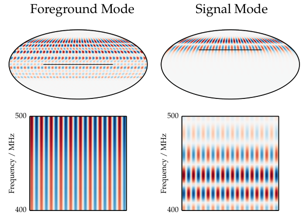
For the purpose of power spectrum estimation (see next section) we will only require forward estimators (where we project quantities into the KL-basis) and knowing will suffice. However, for visualising our results, we want to be able to transform back to the sky (by way of the measured visibilities). This requires us to use an inverse to map from the truncated KL-basis back to the visibilities. Unfortunately because the KL-modes are non-orthogonal it is ambiguous how to project back into the higher dimensional space. One obvious choice would be to make further use of the Moore-Penrose pseudo-inverse. This returns a vector in the visibility space which is a linear combination of the retained signal modes whilst preserving their projected amplitudes. However, because the full set of modes are not orthogonal the resulting vector has a non- zero foreground amplitude (see Figure 7 for a visual illustration).
A far better choice is to generate the full inverse and remove columns corresponding to the rejected modes (we denote this matrix ). This is equivalent to projecting into the full KL-basis, zeroing the foreground contaminated modes, and the using the full-inverse to return the visibility space. The distinction with the pseudo-inverse is shown in Figure 7.

To demonstrate the foreground removal process we project separate realisations of the total intensity foregrounds, polarised foregrounds (showing Stokes Q only), and the signal, through the filtering process (see Figure 8). We show the original simulations, and the maps made from the foreground filtered visibilities. This illustrates how the foreground amplitude is dramatically reduced by the process, whilst the signal retains its overall character.
VII.3 Double-KL transform
So far we have neglected the effects of instrumental noise. To add the instrumental noise back in we simply transform all noise contributions into the new basis. Writing the total noise contribution as , the matrix in the truncated basis is
| (67) | ||||
| (68) |
Though this transform ensures that our foreground contamination remains minimal, as the transformed instrumental noise matrix will not remain diagonal this gives a correlated component between all our modes. However, for further analysis it will be particularly useful if the set of modes we use in our calculation are uncorrelated. By making a further KL-transformation on the foreground removed signal , and total noise covariance matrices, we find a new transformation matrix which maps into a basis where this is true. We will apply a further cutoff to this, including only modes with a signal to total noise ratio greater than to give a transform .
For notational convenience we will write the total transformation in terms of a single matrix , having chosen suitable values for the two cutoffs and . Quantities in this final basis we denote with tildes, for example a visibility mapped into this basis is , and a covariance is . We will denote the signal covariance , and the total noise covariance (including foregrounds) as .
VIII Power Spectrum Estimation
In cosmology we are primarily interested not in the individual structures we see, but in their global properties. It is these statistical observations which tell us about the fundamental nature of the Universe. The quantity we are most interested in is the power spectrum which encodes most of the cosmological information in its shape and evolution. In particular for intensity mapping it allows us to measure the position of the Baryon Acoustic Oscillations (BAOs), which in turn can shed light on the time evolution of dark energy [21].
In order to determine the power spectrum shape we first need to parameterise it. We choose to model the two-dimensional, real-space comoving power spectrum, describing it as a linear summation of different basis functions
| (69) |
In this paper we decompose -space into bands in and , such that each band represents a ring around the line of sight axis in the full three dimensional -space.
We can calculate the accuracy we could achieve measuring the power spectrum using the Fisher Information Matrix, which provides a method for predicting our ability to constrain arbitrary sets of parameters, and has become the essential tool in cosmology for forecasting. The Fisher matrix is defined as
| (70) |
where is the Likelihood function and the are the parameters we are trying to forecast. In the limit that we are measuring the Fisher information for the true parameters that generate the data , and the priors are uniform in this region, the inverse gives a lower bound on the errors of any unbiased estimator (the Cramér-Rao bound), and can be viewed as a forecast for the covariance of the .
Let us specialise this to the case of estimating the power spectrum. After projection into the foreground cleaned basis we assume that the remaining modes follow a complex Gaussian distribution with zero mean. This assumption should be reasonable provided we have successfully removed the modes containing any significant foreground contribution—it is these modes which contain the most non-Gaussian contributions. In this case the Fisher Information matrix of a single -mode for a set of parameters is
| (71) |
where is the linear response of the data covariance to a change in , that is
| (72) |
For power spectrum forecasting, the are the amplitudes of our power spectrum bands (see Equation 69). To calculate the response we need to project the band functions into the cleaned basis. First, the spatial representation must be turned into a multi-frequency angular power spectrum . We do using a simple linear flat-sky prescription which both includes the effects of redshift distortion and structure growth (see Appendix C). We denote the matrix representation of the angular power spectrum basis function as . This must be projected into the KL-basis
| (73) |
In practice explicitly calculating the this way is computationally very expensive. We will discuss a fast Monte-Carlo alternative for calculating the Fisher matrix later in this section. In the constructed eigenbasis is exactly diagonal, however, can have off-diagonal elements.
As there is no coupling between them, the total Fisher Information for the whole dataset is simply the sum over the individual -modes
| (74) |
The Fisher matrix gives us the ability to forecast how well we can possibly measure the power spectrum, but it does not tell us how to go about estimating that power spectrum. We will use the quadratic power spectrum estimator of [52, 53]. This is an optimal estimator in that it achieves the Cramér-Rao bound giving it the lowest possible variance. We will give an overview of this estimator below, though we encourage the reader to look at the original papers for more detail.
As our dataset is made up of a large number of independent -modes, for simplicity we will start with the power spectrum estimator for the whole dataset, and then break it down into individual modes which can be calculated simply.
For notational simplicity, it is most convenient to start with a related estimator
| (75) |
where the quantities on the right hand side include all ’s. This forms a weighted combination of all the quadratic pairs . Our actual power spectrum estimator is built out of linear combinations of the -estimator.
| (76) |
In this subtracts the additive bias from the instrumental and foreground noise, and the mixing matrix takes linear combinations such that is related to the actual power spectrum. Our estimator will have minimum variance with the choice
| (77) |
where again these matrices include all ’s. For a detailed derivation of this weighting, see [52]. Requiring to be an unbiased estimator of the power spectrum we can determine the noise bias term
| (78) |
Our remaining choice is that of the mixing matrix which gives the exact link between our estimator, and the the ‘true’ power spectrum. In particular, we care about the expectation of the estimator
| (79) |
which we have written in terms of a window function which mixes the power spectrum bands. Using Equation 75 and Equation 77 we find that
| (80) | ||||
| (81) |
and combining this with Equation 79, gives the window function as
| (82) |
We fix the normalisation by requiring that . Our choice of the mixing matrix also affects the covariance of the estimator, giving
| (83) |
where we have used the fact that .
There are three common choices for the mixing matrix [54]:
- Unwindowed
-
Choosing the window function to be the identity means that . This corresponds to . This is the most natural choice, however it gives highly correlated errors bars.
- Uncorrelated
-
To make the estimator covariance, we choose . This leads to uncorrelated estimates, but leads to mildly spread window functions [31].
- Minimum Variance
-
The minimum variance estimator requires that the mixing matrix is diagonal , and gives window functions with moderate spread.
We are generally interested in the Unwindowed estimator and we will use this in our forecasts, however, for convergence reasons that we discuss later, we will also use the Minimum Variance estimator when estimating power spectrum biases.
Naive calculation of this estimator is problematic because of the large dimensionality of the data. However, we can trivially exploit the independence of the individual -modes to simplify this calculation. Noting that the covariance matrices in Equation 77 are block diagonal in because they are statistically independent, the weight matrix is also block diagonal. This means we can rewrite the q-estimator as a sum of seperate estimators for each
| (84) |
with
| (85) |
where the are the diagonal blocks of , and is the data for each -mode. Similarly we will also break up the bias terms into contributions from each . The total bias
| (86) |
where the individual
| (87) |
Unfortunately exact calculations of the Fisher matrix and the bias are computationally difficult. While many aspects of the calculation can be simplified by the fact that is diagonal, the need to explicitly construct covariances of and in the KL-basis is still prohibitive. To avoid this, we follow [54, 31] and construct a Monte-Carlo scheme to evaluate the Fisher matrix.
The key to this scheme is that evaluating the -estimator is quick as we do not need to explicitly construct any large matrices. This is achieved by constructing the intermediate vector
| (88) |
which can be efficiently evaluated from right to left. The -estimator is then
| (89) |
As is block diagonal in this can be quickly evaluated. To estimate the Fisher matrix we draw many random realisations of our dataset to which we apply the -estimator. Then, noting that the covariance of is
| (90) |
we can evaluate the sample covariance of our -samples to form an estimate of the Fisher matrix. The estimate the bias term we use the fact that
| (91) |
and take the average of the -estimator under random realisations of the noise.
This Monte-Carlo scheme converges rapidly enough that it is effective for forecasting. Unavoidably there will be small off diagonal terms in the Fisher matrix which do not converge exactly, and these errors can become amplified when taking powers to construct the mixing matrix . These errors remain small enough that they are not apparent when performing power spectrum estimation on data close to the fiducial model, and in most cases this Monte-Carlo technique is still sufficient. However, for data significantly biased from the fiducial model (by – times the estimator error bar) these errors can add spurious noise to the estimator. This is particularly acute when using the Unwindowed estimator which requires the inverse of the Fisher matrix. However, using the Minimum Variance estimator, which does not require us to calculate any powers of the Fisher matrix, alleviates this problem. This is the route we take when dealing with the biased data we will find in Section X.
IX Discussion
IX.1 Polarised Foreground Removal
Foreground cleaning inevitably throws away measured information about the sky, and is guaranteed to reduce our sensitivity to the signal we are seeking. As our primary interest is to measure the power spectrum it is vital that we understand how foreground cleaning methods affect our power spectrum errors. Over the previous sections we have developed the tools to tackles this: in Section II we saw how the -mode formalism gives us a simple and efficient description of the measurement process; Section VII developed an effective foreground cleaning method based on the KL-transform that allows us to easily tracks the statistics of our data through the cleaning; and in the previous section (Section VIII) we constructed an optimal estimator for the power spectrum, and forecast its errors using the Fisher matrix. Here, we combine these to forecast the performance of our example telescope in the presence of foregrounds.

In Figure 9 we show the power spectrum errors for observations of the band with our example telescope. We forecast three distinct sets of foregrounds: no foregrounds; completely unpolarised foregrounds; and partially polarised. We use values of the foreground amplitudes and spectral correlation that are representative of those in our galaxy, these models are described in detail in Appendix C. In particular the latter includes the effects of Faraday rotation, especially emission from a range of Faraday depths within our galaxy, that produces significant spectral structure in the polarised emission.
Clearly the dominant effect of foreground removal in both cases is that we become insensitive to power at low , with a slight increase in the errors across -space. This is in line with our expectations that the foregrounds contaminate the large scale frequency modes corresponding to small , though we discuss this how this relates to the foreground wedge of [55, 29] later.
Polarised foregrounds are removed primarily by the action of the SVD filter described in Section VI. This leads to only a slight worsening of the errors compared to the case of unpolarised foregrounds only. One concern could be that the SVD filter does not discriminate between polarised modes on the basis of the magnitude of their contamination (as would be done by a KL-based filter), it removes them all. This approach is not perfectly optimal, and could be improved by allowing all polarisation modes to propagate through and let the KL-filter determine which to remove. In tests on smaller examples, this approach yields no significant improvement, but due to computational limitations can not be demonstrated on the example in this work.
In all the cases illustrated in Figure 9 there are clear peaks in the sensitivity in the direction that correspond to those seen in Figure 3, and a rapid drop-off as we approach the limit of resolution limit of the telescope. Additionally at low we can see there is a reduction in sensitivity caused by the sample variance of the small number of large scales angular modes.
IX.2 Foreground Wedge
Previous studies of the performance of experiments in the face of large astrophysical foregrounds have found the bulk of the contamination to lie in a wedge shaped region of (for an experiment dependent constant ), termed the foreground wedge [56, 29, 55]. In these studies, the complement of this region remains largely free of contamination, and is thought to provide the best chance for observing cosmological radiation (in the context of Epoch of Reionisation observation this region is called the EoR Window).
Important progress has been made in recent years understanding the source of this contamination [29, 55]: spectrally smooth radio emission is observed at a delay which depends on the baseline length, and distance of the emission from the phase centre, the phase rotation with frequency from this delay appears like fluctuations along the line of sight. This argument leads us to predict that spectrally smooth sources contribute power within a region
| (92) |
where is the comoving distance to redshift , and is the maximum observable distance from the beam centre.
In Figure 9 we mark the boundary of the foreground wedge for our example telecope. While foreground removal makes us insensitive to small there is no discernible variation of this with , and we can observe well into the ‘foreground wedge’. Clearly there is no fundamental loss of information about the entire wedge. Though the distinction between the information lost here, and the whole wedge is small for our example, for a larger telescope with higher angular resolution the difference will be significant.
As pointed out in [33] we expect the foregrounds along each line of sight to be described by only a small number of eigenmodes (with those beyond five contributing less than in power). Though mode-mixing may make these modes appear to contribute power throughout the foreground wedge, fundamentally there are only a small number of them. The KL-transform projects these eigenmodes forward into the data-basis while keeping track of how their angular structure correlate different baselines. If our knowledge of the telescope is perfect, we can use these modes to exactly project out the large foreground contributions to the data.
If our knowledge of the telescope is not perfect as in our forecasts (e.g. Figure 9), we cannot perfectly remove the foregrounds. We investigate this in the following section.
X An Uncertain World
So far we have demonstrated that the signal can be separated from the astrophysical foregrounds in a way which does not distort our measurement of the underlying power spectrum. This assumed an ideal instrument about which our knowledge was perfect in every sense, conditions that a real telescope will not meet. There are many sources of non-ideality — primary beam response, amplifier gains, cable delays and noise temperatures are just a few — each of which could distort our measurements. We can divide these non-idealities into two classes:
- •
Known deviations from the design can be incorporated into our analysis to keep it unbiased and optimal, though our ultimate sensitivity may change relative to the design.
- •
Unknown deviations from our best model of the instrument cannot be corrected and will lead to bias from both foreground leakage and using a biased power spectrum estimator.
The second class of deviations is the most serious, and so for these effects we would like to know how large our uncertainty can be before it matters, or more precisely before it is significant compared to the statistical errors.
As our ability to separate signal and foregrounds requires detailed knowledge of our instrument, we can form a naive expectation of the allowed uncertainty from the dynamic range between signal and foregrounds. In the smooth frequency modes where foregrounds dominate, they are around times brighter than the ( versus ), and so we expect that knowing our instrumental gains and beam shapes to accuracy should be sufficient.
In this section we aim to test two particular forms of uncertainty that we can parametrise simply in our model telescope to see if the requirements are as stringent as . Our approach is to assume that our example telescope represents our best knowledge about the state of the system, which we use to generate our foreground cleaning filter and our power spectrum estimator. We then generate a corrupted timestream corresponding to the observations the true telescope would make. By analysing this timestream with the filters generated for the example telescope we can see at what point imperfect knowledge leads to significant power spectrum biasing.
X.1 Gain Fluctuations
A receiver system turns the input antenna voltage into a signal which can be measured and correlated. In the process of doing this a complex gain may be applied, and while this can be corrected for, this generally leaves unknown residuals in the data. This gain residual is unique to each feed and may be time and frequency dependent.
We model gain fluctuations on a feed by feed basis, as a complex perturbation around a nominal gain of unity. The perturbed feed input is
| (93) |
where the perturbation is a complex Gaussian random variable with variance . These combine to give corrupted visibilities
| (94) |
In our model we do not allow the gain to fluctuate in frequency, enforcing each antennas gain to be frequency independent. However, we do allow the gains to fluctuate in time, assuming that each sample has a separate uncorrelated gain residual. Over the two years of integration, the errors on each co-added sample are reduced by a factor of .
We start with the base timestream to which we have added random gain fluctuations with , and in each period. These time streams are then analysed with the fiducial analysis products that assume no gain fluctuations. In Figure 10 we show the power spectrum biases corresponding to each level of gain fluctuation. We have used the Minimum Variance estimator discussed in Section VIII, the results appear similar if we use the Unwindowed estimator (albeit noisier). The bias, which is caused by foreground leakage from the imperfect calibration, is mostly located within the foreground wedge. This is inline with our expectation from [55, 29] which indicate that leakage from imperfect foreground cleaning will be concentrated in this region. However, there are significant discrepancies from this picture that seem to be related to the array geometry (such as the line ), that may require more detailed study to understand intuitively [57].

We can see that the bias becomes negligible for errors residuals of around . Over the course of the two years observation this corresponds to a tolerance on gain fluctuations of for each synthetic beam (). This required tolerance is significantly less than the naively expected. This difference is due to the fact that we repeatedly measure the same sky because our array is highly redundant (with typical redundancies of ) allowing us to average down the affect of gain fluctuations, reducing the precision required on an individual baseline.
This level of precision should be achievable with techniques such as redundant baseline calibration [58]. Our analysis assumes that the residuals are Gaussian and independent in time, such that they quickly average down with repeated measurements. In practice there may be a component of the residuals from noise with large correlation times which make this assessment more difficult. We leave investigation of such effects for future studies.
X.2 Unknown Primary Beam
One of the key inputs to our analysis is an accurate model of each feeds primary beam. In particular we need the electric field response at each position on the sky, given by the quantity . Generally this quantity can only be determined by calibrating from observations of the sky (for instance by holography). As this process is challenging and time-consuming, we would like to know how precise the calibration must be.
Here, we use the parametrisation of the primary beam given in Section IV.1. We use the fiducial model of the dipole’s beam, , (this is the same as the example used throughout). However, we will perturb the E-plane widths of each antenna around the fiducial model by an amount . Increasing has the effect of making the primary beam of the -feed slightly narrower, and the -feed longer (decreasing it does the opposite). It also reduces the difference in response between the and feeds, reducing the expected amount of polarisation leakage. This is demonstrated in Figure 11 where we show the effect on the Stokes I and polarised response to changes in to the and feeds. In particular we show the derivatives of (Equation 40) and (Equation 41) with respect to and .


To calculate the changes to the data we need to propagate these primary beam changes through to the Beam Transfer matrices. At linear order in the the perturbed Beam Transfer functions are
| (95) |
where the derivatives are related to the primary beam derivatives by
| (96) |
The derivative of the composite beam solid angle is
| (97) |
By treating the primary beam derivatives as a modified beam, we can use Equation 96 to calculate timestreams for the beam perturbed Beam Transfers. We then use Equation 95 to apply the effects of arbitrary combinations of perturbations to for each antenna.
We draw a set of Gaussian distributed values for the width of each feed, . We vary standard deviation (, and of the fiducial model) and use them to generate synthetic data with perturbed beam widths. We propagate the analysis of these corrupted timestreams all the way through to the power spectrum, assuming the fiducial configuration. In Figure 12 we show the results for the Minimum Variance estimator. Again we see that the bias is mostly concentrated in the foreground wedge region. The bias can be significant (compared to statistical errors) if our beam knowledge is imperfect, though it has mostly disappeared in the case where we know the beam width to .
This analysis suggests that if the beam width were the only varying parameter, in the absence of other bias mitigating techniques, we would need to measure it to accuracy. However, as the beam derivative is typically of order (see Figure 11), this can be seen as a precision of around on the beam itself, similar to the gain fluctuations, and still a lower precision than our expectation of around . We can attribute this to the fact that our power spectrum estimation is dependent on a complicated combination of all the primary beams, and this averages down the fluctuations in the same manner as we expect for the gain fluctuations.
Clearly a realistic description of the beam must contain much more than a simple beam width, but this indicates the accuracy to which we must strive to map the primary beam of each feed. This level of precision will be challenging, though not unprecedented, with similar accuracies achieved by holographic means [59].
XI Full bandwidth forecasts
Experiments such as CHIME are targeted at measuring the evolution of dark energy over a large range of redshift. As an example application of this method we show in this Section forecasts for the example cylinder telescope (similar in size to the CHIME Pathfinder but smaller than full CHIME) across a full octave in bandwidth of , corresponding to a redshift range of –. This is broken up into four sub-bands to illustrate the changes with frequency.

In Figure 13 we show the power spectrum forecasts for each of the four sub-bands. This clearly illustrates the increase in sensitivity as we move to higher frequency, particularly at large where the increased angular resolution combines with the decreased observation distance to dramatically increase the spatial resolution. There is an additional boost at large where the constant frequency corresponds to a decreasing line of sight distance. We can also see how the double peaked structure in sensitivity (discussed in Section IX) changes with frequency, with the peaks moving outwards and broadening as expected from the increasing resolution. However, the drop-off at small barely increases in size as it comes from the contribution of sample variance which does not change with the increased angular resolution (it does shift slightly because a fixed angular scale maps a smaller spatial scale at higher frequency).
The effect of foreground cleaning is similar across all bands, with it removing sensitivity for . We don’t expect the number of modes used to describe the foregrounds along a particular line of sight to vary significantly with the small shifts in frequencies between the bands, and this should translate into a similar loss of power spectrum sensitivity for each band.
To constrain the dark energy equation of state, we will use the measured power spectrum in each band to determine the apparent scale of the Baryon Acoustic Oscillation as a function of redshift. The angular and line of sight scales respectively constrain the transverse comoving distance and the Hubble parameter . These give two distinct probes of the expansion history as a function of redshift. In Figure 14 we illustrate how measurements from our example telescope could be used to improve current constraints from Planck.
In Figure 15 we show the predicted constraints on the dark energy equation of state in the - parametrisation. We describe how these are derived from the power spectrum forecasts in Appendix E. This gives a Figure of Merit (FoM) [62] of for the telescope and Planck, and if we add in Stage II experiments. This is an improvement by around from Planck and Stage II only (FoM of ). If there were no loss in sensitivity due to foreground cleaning, the FoM increases to and respectively.
XII Conclusion
In this paper we have improved and extended the -mode formalism for analysing observations from transit radio interferometers. In particular, we have extended the formalism to include a complete description of polarisation (see Section II). This allows us to characterize observations of the real polarised sky including the effects of instrumental polarisation. Including these effects is crucial when making wide-field multi-frequency observations with a polarization-dependent sky response. Furthermore, by considering the geometry of the measured data in the vector space of observations, we have developed a simple SVD projection that not only yields a significant data compression, but also acts as an effective filter to suppress polarised foreground contamination (Section VI).
In the limit of statistically isotropic foregrounds, each -mode is independent of the others with no statistical coupling between them. Thus the -mode formalism, because it allows each mode to be treated independently, allows for a compact and computationally efficient representation for statistics of our data. We have exploited this to develop the KL-transform as a technique for the removal of of astrophysical foregrounds, which otherwise appears to be extremely challenging using other methods (Section VII). We believe this is the first technique shown to be effective at the removal of polarised foregrounds to below the signal level while using a telescope model with realistic amounts of polarisation leakage (see Figure 8).
Within the -mode formalism we have constructed an optimal quadratic estimator for the power spectrum that is computationally efficient and takes into account the full statistics of the data, including the effects of the foreground cleaning (Section VIII). This has allowed us to forecast the performance of a medium sized cylinder transit telescope (Section IX) — similar in size to the CHIME pathfinder telescope currently under construction. We show that the KL-transform is able to clean foregrounds well into the foreground wedge, demonstrating that there is no fundamental information loss within the region, with foreground cleaning limiting our measurements only in a smaller band . In fact, we find that even the removal of the polarized foregrounds gives a minimal reduction in the expected ability to constrain the power spectrum.
While our results are encouraging, the -mode formalism does make simplifying assumptions and the impact of these assumptions needs to be tested when analysing real experiments. For instance, for the analysis to be tractable, we assume the statistics of the data are stationary under rotation of the Earth. This is expected of the signal itself, but is not expected to be true of both for the foregrounds where the galaxy is heavily anisotropic (though in our simulations this does not seem prevent us from suppressing foregrounds consistent with the actual structure of the galaxy), and for the instrumental effects where noise, RFI, and thermal fluctuations make the behaviour the of the instrument time dependent. The -mode formalism also assumes perfect knowledge of the telescope, including amplifier gains, and fully characterised beams. In Section X we have investigated how these uncertainties, if ignored, would lead to significant biases in the measured power spectrum, and placed limits on how well we must know these to faithfully recover the power spectrum. We find that random complex gain variations can have an amplitude of up to (on one minute timescales), before they cause any significant power spectrum shifts. Similarly, using the beam width as a simple parameterisation of our uncertainty we find that we must know the width of the primary beam of each feed to around to avoid bias. These precisions are less stringent than naive expectations from the dynamic range between the signal and foregrounds (around ). Though challenging, requiring effort and innovation, they should be achievable.
One avenue to further loosen these calibration requirements is to follow the same philosophy we take with foreground removal and conservatively identify, and remove, the modes which are particularly susceptible to this miscalibration. Even in the case where we perturb the nominal beam width by an unknown number of order there is a significant fraction of the KL modes that do not get biased appreciably. It is conceivable that through Monte-Carlo modelling of beam uncertainties the highly corruptible KL modes could be found and excised prior to estimating the power spectrum (at the cost of increased error bars). Alternatively we could pursue a more targeted approach by incorportating these instrumental uncertainties into the noise model, and using the KL-filter to remove them. We leave investigations of these and other bias mitigating techniques to future work.
When our feed spacing is larger than the Nyquist criterion at a particular wavelength (for a beam stretching to the horizon this is ), we cannot uniquely localise a source on the sky. This aliasing effect causes us to form multiple images when map-making and, while not leading to biases, gives a degradation in power spectrum errors. For the example cylinder telescope used here, this occurs at . While an investigation of this effect is beyond the scope of this paper we do not expect it is a fundamental limitation and believe that this degradation may be alleviated by moving away from a fully uniform feed spacing.
The pipeline we have developed for performing the -mode analysis described in this paper is publically available from http://github.com/radiocosmology. The tools created for modelling and simulating the radio sky are available from the same location.
Acknowledgements.
We thank the CHIME team for stimulating discussions. KS, UP, and MS are supported in part by the Natural Sciences and Engineering Research Council (NSERC) of Canada. The work of AS was supported by the DOE at Fermilab under Contract No. DE-AC02-07CH11359. KS thanks Perimeter Institute for Theoretical Physics for their hospitality. Some of the results in this paper have been derived using the HEALPix11 1 http://healpix.sourceforge.net/ package [63]. Computations were performed on the GPC supercomputer at the SciNet HPC Consortium. SciNet is funded by: the Canada Foundation for Innovation under the auspices of Compute Canada; the Government of Ontario; Ontario Research Fund - Research Excellence; and the University of Toronto.Appendix A Noise Power Spectrum
The sensitivity of a a radio receiver is a well studied problem [46, 64, 65]. For a single feed the power received in a frequency interval is simply related to the antenna temperature (in the absence of noise). In our notation the antenna temperature for a single feed is simply equal to its auto-correlation . However, we need to extend this to the case of the correlation of two separate antennas. Provided that the power for both the auto-correlation and cross-correlation cases, the signal observed is
| (98) |
where the real and imaginary parts of contain the cosine and sine-like correlations. The same conclusion can be reached by following through the correlation of the induced voltage from each antenna using the effective length. With our normalisation , with the maximum length anywhere on the sky.
Beyond the astrophysical signal there are other contributions to the observed power. This noise may come from many sources such as the ground or the atmosphere, or the receiver system itself. For the auto-correlation of a single feed the instantaneous noise power defines the system temperature
| (99) |
When consider the cross-correlation between different feeds, provided the noise at both is uncorrelated, there is no additional power observed in the mean of the signal. However, the noise does contribute to the fluctuations about the mean. If we average a frequency channel of width over a rectangular window of time length , we find the mean power observed is
| (100) |
The fluctuations in the amplitude have standard deviation
| (101) |
See [64, 65] for a detailed calculation. The fluctuations in the real and imaginary have an equal amplitude of . We have assumed we are in the limit where the the system temperature dominates the antenna temperature, .
If the noise at each feed is independent, that means that the noise between different baseline pairs is uncorrelated. The variance that we would ascribe to the measurement of a particular visibility at a particular time (after the averaging) is
| (102) |
To calculate the -mode power spectrum of fluctuations we first calculate the noise correlation function. Assuming that it is white noise, and again using a rectangular window function the correlation function is
| (103) |
where the triangle function for . To calculate the noise power spectrum we simply fourier transform this quantity. As we need to consider the problem in terms of Earth rotation, we identify distinct sidereal days as independent measurements of the sky and treat the averaged noise as periodic. Similarly we can identify redundant baselines, as independent measurements of the same quantity. Only the diagonal elements of the noise matrix, corresponding to the same frequency and baseline are non-zero. The discrete power spectrum of the noise, defined by , is
| (104) |
where is the number of sidereal days that have been observed. Usually we would want the integration length to be smaller than any angular scale we are interested in, in this limit , and the factor is .
Appendix B Karhunen-Loève Transform
Let us write our measurement as a vector , where the each dimension corresponds to a measured degree of freedom. We can write as
| (105) |
where and are respectively the signal we are interested in and some generalised form of noise (in the case of this may include the foregrounds). These components have covariance matrices
| (106) |
We are free to transform the measurement vector as we wish, , provided we are careful to update all the statistics we make use of. In our case we are interested in the two point statistics and so it is sufficient to transform the covariance matrix . The Karhunen-Loeve (KL) transform takes advantage of this to produce simultaneous eigenmodes of the signal and noise covariances.
We start by making the eigendecomposition of the noise matrix
| (107) |
where is the unitary matrix of eigenvectors (stacked row by row), and is the diagonal matrix of eigenvalues. Using this we can transform the data vector , which produces a new signal covariance
| (108) |
and reduces the noise matrix to . As the new noise matrix consists solely of positive diagonal elements , a further transformation , where , reduces the noise matrix to the identity . The signal matrix is transformed to
| (109) |
Applying any unitary transformation to the data will leave the noise covariance as the identity. We use this freedom to diagonalise the signal covariance by eigendecomposition , leaving the total transformation on the data as
| (110) |
Overall this has changed the covariance matrices to
| (111) | ||||
| (112) |
By making this transformation we have simultaneously diagonalised the correlations of both the signal and the noise, mapping the latter to the identity matrix. In particular, the elements of give the signal to noise ratio of each mode. With no hidden correlations this basis allows us to cleanly filter data by simply throwing away modes with signal to noise ratio below some threshold. This is equivalent to zeroing the corresponding elements of .
Rather than explicitly constructing the three transformations, it is mathematically equivalent to find the solutions to the generalised eigenvalue problem
| (113) |
with the eigenvectors forming the transformation matrix, and the eigenvalues giving the elements of the signal covariance . This approach is simpler and computationally more efficient.
Appendix C Statistical Models
As discussed in Section VII to use the Karhunen-Loève transform to perform foreground cleaning we require models of the two-point statistics of both the signal and the foreground contaminants. For computational efficiency these models must be isotropic and so we only need to specify the angular power spectrum
| (114) |
for all the pairs of the four polarisation components .
C.1 Astrophysical Foregrounds
Our foreground models are based on [48]. However we only include the dominant two components, the galactic synchrotron emission and extragalactic point sources. In both cases the angular power spectrum is of the form
| (115) |
The original models were calibrated for forecasting observations of Epoch of Reionisation. In [32] we recalibrated them for the high frequency, all sky observations we are concerned with in this paper. However for this work we also need to specify the correlations of the polarised parts of the foregrounds. We assume that the dominant source of polarised emission is our own galaxy (ignoring the polarisation of point sources) and model the polarised emission as being a statistical fraction of the unpolarised emission
| (116) |
In addition we assume that the polarised emission is uncorrelated such that , and that there is no circular polarisation from the galaxy . Our fiducial polarisation fraction is . We list the parameters for these models in Table 2.
| Component | Polarisation | A () | |||
|---|---|---|---|---|---|
| Galaxy | TT | ||||
| EE, BB | |||||
| Point Sources | TT |
C.2 21 cm Signal
On large scales the brightness temperature is a biased tracer of the matter density field [66] with a power spectrum given by
| (117) |
where is the bias and is the real-space matter power spectrum. The evolution of the perturbations is given by the growth factor normalised such that , with the growth rate (that is the logarithmic derivative of the growth factor ). The mean brightness temperature is assumed to take the form
| (118) |
given in [1]. In [67] they determine the degenerate product , which we use in this work. As the redshift distortions break the degeneracy we fix .
For use in our foreground filter, we require the angular power spectrum of the brightness temperature [68, 69]. This can be calculated from the real-space power spectrum Equation 117, but is compuationally difficult, generally requiring double-integration over highly oscillatory functions for each , pair. To speed this up we use the flat-sky approximation from [69]
| (119) |
where and are the comoving distances to redshift and and their difference is denoted by . The wavevector has components and in the directions parallel and perpendicular to the line of sight ( is the mean of and ). This approximation is accurate to the 1% level for [69].
We use this method not only for calculating the signal covariance function, but also the band functions required for the power spectrum. To determine each we simply apply Equation 117 and Equation 119, with .
Appendix D Simulating All-sky Radio Emission
Testing of the -mode formalism, and the foreground cleaning with the Karhunen-Loève transform requires the use of synthetic sky maps. For it to be realistic these simulated maps must capture the essential properties of the signal and foreground components. In this Section we briefly describe how these simulations are generated.
D.1 21 cm Signal
Assuming the cosmological emission is Gaussian on the scales of interest, the angular power spectrum given in the previous section (Equation 119) completely specifies its fluctuations. Maps of the sky can be generated by drawing Gaussian realisations of the power spectrum, using Cholesky decomposition to produce the correct frequency correlation structure, and then adding in the mean temperature given by Equation 118.
D.2 Extra-Galactic Point Sources
We construct our point source simulations from three components: a population of real bright point sources ( at ); a synthetic population of dimmer sources down to at ; and an unresolved background of dimmer sources () modelled as a Gaussian random field. This last component dramatically reduces the number of sources we must directly generate.
The unresolved background is generated by drawing a Gaussian realisation from the point source model detailed in Table 2. The random source catalogue is constructed by drawing from the point source distribution of [70] and scattering the sources randomly over the sky. The intrinsic polarisation of each point source is determined by
| (120) |
where the polarisation fraction is a complex Gaussian random variable with standard deviation . This standard deviation is equal to the average polarisation fraction of sources in the catalogue, we set .
The population of real bright point sources is generated by matching VLSS at [71] against NVSS at [72]. We only include sources interpolated to be brighter than at . Each source is assigned the polarisation as measured by NVSS, and is extrapolated to other frequencies. In this work we have also assumed that the six sources above (at ) have been removed from the timestream to high accuracy.
The polarisation of an extra-galactic source is Faraday rotated as it passes through the magnetised interstellar medium in our galaxy, generating oscillatory frequency structure in the polarisation. To apply this, we use the Faraday depth map of [73] to rotate the polarisation angle of our background sources.
D.3 Galactic Synchrotron Intensity
In this work we continue to use the prescription developed in a previous paper [32] to generate constrained simulations of the total intensity of synchrotron emission from our galaxy. These maps are formed from two distinct components:
- •
A large scale base map produced by extrapolating the Haslam map22 2 We use the map from the Legacy Archive for Microwave Background Data Analysis (LAMBDA), which has been processed to remove bright point sources and striping. See http://lambda.gsfc.nasa.gov/product/foreground/haslam_408.cfm with a spectral index map from [74].
- •
A randomly generated map that adds in fluctuations in frequency and on small angular scales. This is constrained to be zero on the scales constrained by the Haslam map, and is designed to smoothly extrapolate the angular fluctuations of the Haslam map to smaller scales, and reproduce the anisotropic fluctuations on small scale power across the sky [75].
The procedure for generating these two components is described in detail in [32], with the only change being the spectral index map used.
D.4 Galactic Synchrotron Polarisation
To test our foreground removal and analysis we need to be able to create simulated multi-frequency maps of our galaxy, and in particular its polarisation structure. As the observed radiation has been omitted across a range of Faraday depths, unlike extra-galactic sources, this is challenging. One approach is to make use of the increasingly sophisticated models of the galactic magnetic field structure [76], and electron distribution [77], to create realistic large scale simulations of the polarisation structure [78]. However, we instead appeal to the ideas of Faraday Rotation Measure Synthesis [79] to rapidly create simulations that capture the important effects.
Rotation measure synthesis attempts to link the wavelength dependent polarisation rotation to the structure along the line of sight. Polarised radiation emitted at a distance from us is Faraday rotated by an amount before it reaches us, where the Faraday depth
| (121) |
The key idea in Faraday Rotation Measure Synthesis is to not directly probe the physical structure of emission, but to probe the structure as a function of Faraday depth. In this case we can just think of the observed polarised emission in a given direction as being the summation of the emission at all Faraday depths , rotated by the correct wavelength dependent amount
| (122) |
In [79] the idea was to use multi-wavelength observations to invert this Fourier relation, and constrain the structure of . However, we will attempt to use well motivated assumptions about the emission in Faraday-space to construct simulations of polarised skies. As in [79] we presume that the Faraday space emission is separable in its spectral dependence, such that . This flattens the spectrum of so that we can still use the Faraday synthesis formalism for it. We take the spectral function from the unpolarised emission.
We start with a simple model of the emission from the galaxy, assuming that along any line of sight the emission comes from many independent synchrotron regions each of fixed brightness . In a direction with total brightness temperature , there are such regions. We assume that the emitting regions are scattered across a range in Faraday depth. With no reason to favour positive or negative Faraday depths, we assume this distribution is zero mean. From observations of extragalactic point sources we know the Faraday depth to the edge of our galaxy [73] and this gives us a measure of the range of Faraday depths within the galaxy. Combining these properties the distribution is modelled as a zero-mean Gaussian with a width which is determined from the Faraday rotation data. We determine by taking the Faraday depth map of [73], taking its absolute value, and smoothing with a FWHM of . Each of these regions has a small width in over which its polarisation is coherent. We call this coherence length , and note that it determines size of structures in Faraday space
To determine the polarisation structure we start by calculating the number of emitting regions within a range to . This is given by
| (123) |
As each region is independent we assume they have a randomly distributed complex polarisation, drawn from a Gaussian distribution with variance , where is the polarisation fraction. Within this range in Faraday depth the polarisations add up like a random walk, giving the expected total root-mean-square polarisation as
| (124) |
This gives the expected magnitude of the emission at each position in Faraday space, showing that even in Faraday space we see depolarisation because of the incoheret combination of multiple Faraday sources at a single depth.
This suggests we model the emission as two factors
| (125) |
The first is a positive envelope function which defines the region, and amplitude of emission in Faraday depth.
| (126) |
The second is a random field that gives fluctuations in the complex polarisation as a function of Faraday depth, this should be highly correlated on scales , and uncorrelated on scales . We model this as a Gaussian random field drawn with an angular power spectrum
| (127) |
The angular dependence is chose to match that of the total intensity model Equation 115.
The normalisation of these functions is degenerate with the value of . We fix the combination by considering what happens at high frequency observations where Faraday rotation is much less important. In this limit the polarisation fraction is determined by the incoherent addition of the polarisation of the emitting regions and is . We choose which is the intrinsic polarisation of synchrotron with a spectral index of the electron energy distribution . Polarised maps from the WMAP satellite at [80] indicate that the galaxy is 20% polarised at high latitudes, we use this fact to determine the overall normalisation.
The only remaining degree of freedom is the the correlation length of the emitting regions if Faraday space, . The size of an emitting region in Faraday space will grow towards the galactic centre because of the increased magnetic field strengths. We construct a crude model
| (128) |
chosen to visually reproduce the amount of depolarisation seen in polarisation maps [81, 82, 83].
This gives all the necessary ingredients to draw a realisation of which we can Fourier transform, and scale by the spectral function to produce the polarised emission using Equation 122. All these operations are performed on a regular grid in , which is extended beyond the desired frequency range to negate edge effects. The resulting series of maps are then interpolated onto the required frequency slices.
Polarisation Fraction

Correlation length

In Figure 16 we show the polarisation fraction, and frequency correlation length derived from a simulation between . Though the model we have constructed here is crude, and based unrealistic assumptions about the galactic emission it exhibits the properties we would expect from the real galactic emission:
- •
Emission is from a range of Faraday depths, rather than a single screen.
- •
In the galactic plane there is substantial depolarisation, but at high latitudes the polarisation fraction is around that at .
- •
Frequency decorrelation on lengths that we would predict from the Faraday rotation over the galaxy, going to near zero in the galactic centre where the emission goes up to large Faraday depths.
Appendix E Distance Measurements
By extracting the Baryon Acoustic Oscillation (BAO) signal from the power spectrum, measurements of the Hubble rate and transverse comoving distance can be made. The BAO manifests itself as a preferred separation in the two-point correlation function at distances perpendicular to the line of sight and parallel to the line of sight. The fractional errors on and are equivalent to the fractional errors on the combinations and , respectively, where is the comoving sound horizon at the drag epoch. Thus, if is well-known (for example from observations of the Cosmic Microwave Background) then measurements of and put observational constraints on and .
To project uncertainties in the power spectrum onto and , we first transform the Fisher matrix for the power spectrum into the Fisher matrix for the parameters via the Jacobian , where the Fisher matrices are related by . is evaluated using a fiducial cosmological model.
To calculate , we follow [84], where the effect of the baryons on the power spectrum is modelled by an additive term to the otherwise ‘wiggles-free’ power spectrum that is approximated as
| (129) |
where , is the Silk scale, and is the linear power spectrum evaluated at . In this expression, is a normalization constant, taken to be . is the nonlinear dampening scale given by
| (130) |
where , , is the growth function, and is the growth rate. We follow [85] and assume that we may partially reconstruct parts of the BAO signal degraded by nonlinear effects for modes with high signal to noise and set the effective nonlinear dampening scale to be . By differentiating Equation 129 with respect to the variables , one can form and subsequently evaluate . Note that is equivalent to the Fisher matrix for the variables .
The Fisher matrix can be transformed again into the Fisher matrix for the cosmological parameters by use of the Jacobian , which as before is evaluated using a fiducial cosmological model. In , the equation of state has been parameterized as
| (131) |
Note that the dependence in comes from the comoving sound horizon , present in both terms of , which is dependent on the baryon to photon ratio . The Fisher matrix for the dark energy parameters is then formed as . Constraint contours in the plane can be found by marginalizing over the other variables in , which in this case amounts to inverting to get the covariance matrix, removing the rows and columns corresponding to the marginalized variables, and inverting once more to recover the marginalized Fisher matrix for .
References
- [1] T.-C. Chang, U.-L. Pen, J. B. Peterson, and P. McDonald, Physical Review Letters 100, 091303 (2008), arXiv:0709.3672 .
- [2] A. Loeb and J. S. B. Wyithe, Physical Review Letters 100, 161301 (2008), arXiv:0801.1677 .
- [3] S. R. Furlanetto, S. P. Oh, and F. H. Briggs, Phys. Rep. 433, 181 (2006), arXiv:astro-ph/0608032 .
- [4] A. Loeb and M. Zaldarriaga, Physical Review Letters 92, 211301 (2004), arXiv:astro-ph/0312134 .
- [5] G. Swarup, S. Ananthakrishnan, V. K. Kapahi, A. P. Rao, C. R. Subrahmanya, and V. K. Kulkarni, Current Science, Vol. 60, NO.2/JAN25, P. 95, 1991 60, 95 (1991).
- [6] J. C. Pober, A. Liu, J. S. Dillon, J. E. Aguirre, J. D. Bowman, R. F. Bradley, C. L. Carilli, D. R. DeBoer, J. N. Hewitt, D. C. Jacobs, M. McQuinn, M. F. Morales, A. R. Parsons, M. Tegmark, and D. J. Werthimer, ArXiv e-prints (2013a), arXiv:1310.7031 [astro-ph.CO] .
- [7] M. P. van Haarlem, M. W. Wise, A. W. Gunst, G. Heald, J. P. McKean, J. W. T. Hessels, A. G. de Bruyn, R. Nijboer, J. Swinbank, R. Fallows, et al., A&A 556, A2 (2013), arXiv:1305.3550 [astro-ph.IM] .
- [8] C. J. Lonsdale, R. J. Cappallo, M. F. Morales, F. H. Briggs, L. Benkevitch, J. D. Bowman, J. D. Bunton, S. Burns, B. E. Corey, L. Desouza, S. S. Doeleman, M. Derome, A. Deshpande, M. R. Gopala, L. J. Greenhill, D. E. Herne, J. N. Hewitt, P. A. Kamini, J. C. Kasper, B. B. Kincaid, J. Kocz, E. Kowald, E. Kratzenberg, D. Kumar, M. J. Lynch, S. Madhavi, M. Matejek, D. A. Mitchell, E. Morgan, D. Oberoi, S. Ord, J. Pathikulangara, T. Prabu, A. Rogers, A. Roshi, J. E. Salah, R. J. Sault, N. U. Shankar, K. S. Srivani, J. Stevens, S. Tingay, A. Vaccarella, M. Waterson, R. B. Wayth, R. L. Webster, A. R. Whitney, A. Williams, and C. Williams, IEEE Proceedings 97, 1497 (2009), arXiv:0903.1828 [astro-ph.IM] .
- [9] H. Zheng, M. Tegmark, V. Buza, J. S. Dillon, H. Gharibyan, J. Hickish, E. Kunz, A. Liu, J. Losh, A. Lutomirski, S. Morrison, S. Narayanan, A. Perko, D. Rosner, N. Sanchez, K. Schutz, S. M. Tribiano, M. Zaldarriaga, K. Zarb Adami, I. Zelko, K. Zheng, R. Armstrong, R. F. Bradley, M. R. Dexter, A. Ewall-Wice, A. Magro, M. Matejek, E. Morgan, A. R. Neben, Q. Pan, C. M. Peterson, M. Su, J. Villasenor, C. L. Williams, H.-I. Yang, and Y. Zhu, ArXiv e-prints (2013), arXiv:1309.2639 [astro-ph.IM] .
- [10] A. R. Parsons, D. C. Backer, G. S. Foster, M. C. H. Wright, R. F. Bradley, N. E. Gugliucci, C. R. Parashare, E. E. Benoit, J. E. Aguirre, D. C. Jacobs, C. L. Carilli, D. Herne, M. J. Lynch, J. R. Manley, and D. J. Werthimer, AJ 139, 1468 (2010), arXiv:0904.2334 [astro-ph.CO] .
- [11] J. C. Pober, A. R. Parsons, D. R. DeBoer, P. McDonald, M. McQuinn, J. E. Aguirre, Z. Ali, R. F. Bradley, T.-C. Chang, and M. F. Morales, AJ 145, 65 (2013b), arXiv:1210.2413 [astro-ph.CO] .
- [12] R. Ansari, J.-E. Campagne, P. Colom, C. Magneville, J.-M. Martin, M. Moniez, J. Rich, and C. Yèche, Comptes Rendus Physique 13, 46 (2012a), arXiv:1209.3266 [astro-ph.CO] .
- [13] R. A. Battye, I. W. A. Browne, C. Dickinson, G. Heron, B. Maffei, and A. Pourtsidou, ArXiv e-prints (2012), arXiv:1209.0343 [astro-ph.CO] .
- [14] CHIME, “Canadian Hydrogen Intensity Mapping Experiment (CHIME),” (2013).
- [15] G. W. Kant, P. D. Patel, S. J. Wijnholds, M. Ruiter, and E. van der Wal, IEEE Transactions on Antennas and Propagation 59, 1990 (2011).
- [16] S. Saiyad Ali and S. Bharadwaj, ArXiv e-prints (2013), arXiv:1310.1707 [astro-ph.CO] .
- [17] Parkes, “CSIRO Parkes Observatory,” (2013).
- [18] X. Chen, International Journal of Modern Physics Conference Series 12, 256 (2012), arXiv:1212.6278 [astro-ph.IM] .
- [19] C. Blake, E. A. Kazin, F. Beutler, T. M. Davis, D. Parkinson, S. Brough, M. Colless, C. Contreras, W. Couch, S. Croom, D. Croton, M. J. Drinkwater, K. Forster, D. Gilbank, M. Gladders, K. Glazebrook, B. Jelliffe, R. J. Jurek, I.-H. Li, B. Madore, D. C. Martin, K. Pimbblet, G. B. Poole, M. Pracy, R. Sharp, E. Wisnioski, D. Woods, T. K. Wyder, and H. K. C. Yee, MNRAS 418, 1707 (2011), arXiv:1108.2635 [astro-ph.CO] .
- [20] L. Anderson, E. Aubourg, S. Bailey, D. Bizyaev, M. Blanton, A. S. Bolton, J. Brinkmann, J. R. Brownstein, A. Burden, A. J. Cuesta, L. A. N. da Costa, K. S. Dawson, R. de Putter, D. J. Eisenstein, J. E. Gunn, H. Guo, J.-C. Hamilton, P. Harding, S. Ho, K. Honscheid, E. Kazin, D. Kirkby, J.-P. Kneib, A. Labatie, C. Loomis, R. H. Lupton, E. Malanushenko, V. Malanushenko, R. Mandelbaum, M. Manera, C. Maraston, C. K. McBride, K. T. Mehta, O. Mena, F. Montesano, D. Muna, R. C. Nichol, S. E. Nuza, M. D. Olmstead, D. Oravetz, N. Padmanabhan, N. Palanque-Delabrouille, K. Pan, J. Parejko, I. Pâris, W. J. Percival, P. Petitjean, F. Prada, B. Reid, N. A. Roe, A. J. Ross, N. P. Ross, L. Samushia, A. G. Sánchez, D. J. Schlegel, D. P. Schneider, C. G. Scóccola, H.-J. Seo, E. S. Sheldon, A. Simmons, R. A. Skibba, M. A. Strauss, M. E. C. Swanson, D. Thomas, J. L. Tinker, R. Tojeiro, M. V. Magaña, L. Verde, C. Wagner, D. A. Wake, B. A. Weaver, D. H. Weinberg, M. White, X. Xu, C. Yèche, I. Zehavi, and G.-B. Zhao, MNRAS 427, 3435 (2012), arXiv:1203.6594 [astro-ph.CO] .
- [21] C. Blake and K. Glazebrook, ApJ 594, 665 (2003), astro-ph/0301632 .
- [22] W. Hu and Z. Haiman, Phys. Rev. D 68, 063004 (2003), astro-ph/0306053 .
- [23] H.-J. Seo and D. J. Eisenstein, ApJ 598, 720 (2003), astro-ph/0307460 .
- [24] S. T. Myers, C. R. Contaldi, J. R. Bond, U.-L. Pen, D. Pogosyan, S. Prunet, J. L. Sievers, B. S. Mason, T. J. Pearson, A. C. S. Readhead, and M. C. Shepherd, ApJ 591, 575 (2003), arXiv:astro-ph/0205385 .
- [25] M. Tegmark and M. Zaldarriaga, Phys. Rev. D 79, 083530 (2009), arXiv:0805.4414 .
- [26] A. R. Parsons and D. C. Backer, AJ 138, 219 (2009), arXiv:0901.2575 [astro-ph.IM] .
- [27] A. Liu, M. Tegmark, S. Morrison, A. Lutomirski, and M. Zaldarriaga, MNRAS 408, 1029 (2010a), arXiv:1001.5268 [astro-ph.IM] .
- [28] A. Liu and M. Tegmark, Phys. Rev. D 83, 103006 (2011), arXiv:1103.0281 [astro-ph.CO] .
- [29] A. R. Parsons, J. C. Pober, J. E. Aguirre, C. L. Carilli, D. C. Jacobs, and D. F. Moore, ApJ 756, 165 (2012), arXiv:1204.4749 [astro-ph.IM] .
- [30] R. Ansari, J. E. Campagne, P. Colom, J. M. Le Goff, C. Magneville, J. M. Martin, M. Moniez, J. Rich, and C. Yèche, A&A 540, A129 (2012b), arXiv:1108.1474 [astro-ph.CO] .
- [31] J. S. Dillon, A. Liu, and M. Tegmark, Phys. Rev. D 87, 043005 (2013), arXiv:1211.2232 [astro-ph.CO] .
- [32] J. R. Shaw, K. Sigurdson, U.-L. Pen, A. Stebbins, and M. Sitwell, ArXiv e-prints (2013), arXiv:1302.0327 [astro-ph.CO] .
- [33] A. Liu and M. Tegmark, MNRAS 419, 3491 (2012), arXiv:1106.0007 [astro-ph.CO] .
- [34] A. Liu, M. Tegmark, and M. Zaldarriaga, MNRAS 394, 1575 (2009), arXiv:0807.3952 .
- [35] D. F. Moore, J. E. Aguirre, A. R. Parsons, D. C. Jacobs, and J. C. Pober, ApJ 769, 154 (2013), arXiv:1302.0876 [astro-ph.CO] .
- [36] J. Kim, MNRAS 375, 625 (2007), arXiv:astro-ph/0611410 .
- [37] J. D. McEwen and A. M. M. Scaife, MNRAS 389, 1163 (2008), arXiv:0803.2165 .
- [38] M. A. Holdaway, in Synthesis Imaging in Radio Astronomy II, Astronomical Society of the Pacific Conference Series, Vol. 180, edited by G. B. Taylor, C. L. Carilli, and R. A. Perley (1999) p. 401.
- [39] S. Bhatnagar, T. J. Cornwell, K. Golap, and J. M. Uson, A&A 487, 419 (2008), arXiv:0805.0834 .
- [40] M. Zaldarriaga and U. Seljak, Phys. Rev. D 55, 1830 (1997), astro-ph/9609170 .
- [41] B. Y. Mills, Proceedings of the Astronomical Society of Australia 4, 156 (1981).
- [42] G. Swarup, N. V. G. Sarma, M. N. Joshi, V. K. Kapahi, D. S. Bagri, S. H. Damle, S. Ananthakrishnan, V. Balasubramanian, S. S. Bhave, and R. P. Sinha, Nature Physical Science 230, 185 (1971).
- [43] J. B. Peterson, K. Bandura, and U. L. Pen, ArXiv Astrophysics e-prints (2006), arXiv:astro-ph/0606104 .
- [44] C. Craeye, in Antennas and Propagation Society International Symposium, 2005 IEEE, Vol. 2B (2005) pp. 449–452 vol. 2B.
- [45] C. Craeye, in Antennas and Propagation Society International Symposium, 2008. AP-S 2008. IEEE (2008) pp. 1–4.
- [46] C. A. Balanis, Antenna theory : analysis and design, 3rd ed. by C.A. Balanis. Hoboken, NJ: Wiley-Interscience, 2005, 3rd ed. (Wiley-Interscience, 2005).
- [47] D. Varshalovich, A. Moskalev, and V. Khersonskiĭ, Quantum Theory of Angular Momentum: Irreducible Tensors, Spherical Harmonics, Vector Coupling Coefficients, 3nj Symbols (World Scientific Pub., 1988).
- [48] M. G. Santos, A. Cooray, and L. Knox, ApJ 625, 575 (2005), arXiv:astro-ph/0408515 .
- [49] J. R. Bond, Physical Review Letters 74, 4369 (1995), arXiv:astro-ph/9407044 .
- [50] M. Tegmark, A. N. Taylor, and A. F. Heavens, ApJ 480, 22 (1997), arXiv:astro-ph/9603021 .
- [51] E. F. Bunn, M. Zaldarriaga, M. Tegmark, and A. de Oliveira-Costa, Phys. Rev. D 67, 023501 (2003), arXiv:astro-ph/0207338 .
- [52] M. Tegmark, Phys. Rev. D 55, 5895 (1997), arXiv:astro-ph/9611174 .
- [53] J. R. Bond, A. H. Jaffe, and L. Knox, Phys. Rev. D 57, 2117 (1998), arXiv:astro-ph/9708203 .
- [54] N. Padmanabhan, U. Seljak, and U. L. Pen, New A 8, 581 (2003), arXiv:astro-ph/0210478 .
- [55] M. F. Morales, B. Hazelton, I. Sullivan, and A. Beardsley, ApJ 752, 137 (2012), arXiv:1202.3830 [astro-ph.IM] .
- [56] A. Datta, J. D. Bowman, and C. L. Carilli, ApJ 724, 526 (2010), arXiv:1005.4071 [astro-ph.CO] .
- [57] B. J. Hazelton, M. F. Morales, and I. S. Sullivan, ApJ 770, 156 (2013), arXiv:1301.3126 [astro-ph.IM] .
- [58] A. Liu, M. Tegmark, S. Morrison, A. Lutomirski, and M. Zaldarriaga, MNRAS 408, 1029 (2010b), arXiv:1001.5268 [astro-ph.IM] .
- [59] G. R. Harp, R. F. Ackermann, Z. J. Nadler, S. K. Blair, M. M. Davis, M. C. H. Wright, J. R. Forster, D. R. Deboer, W. J. Welch, S. Atkinson, D. C. Backer, P. R. Backus, W. Barott, A. Bauermeister, L. Blitz, D. C.-J. Bock, G. C. Bower, T. Bradford, C. Cheng, S. Croft, M. Dexter, J. Dreher, G. Engargiola, E. D. Fields, C. Heiles, T. Helfer, J. Jordan, S. Jorgensen, T. Kilsdonk, C. Gutierrez-Kraybill, G. Keating, C. Law, J. Lugten, D. H. E. MacMahon, P. McMahon, O. Milgrome, A. Siemion, K. Smolek, D. Thornton, T. Pierson, K. Randall, J. Ross, S. Shostak, J. C. Tarter, L. Urry, D. Werthimer, P. K. G. Williams, and D. Whysong, IEEE Transactions on Antennas and Propagation 59, 2004 (2011), arXiv:1210.8246 [astro-ph.IM] .
- [60] Planck Collaboration, P. A. R. Ade, N. Aghanim, C. Armitage-Caplan, M. Arnaud, M. Ashdown, F. Atrio-Barandela, J. Aumont, C. Baccigalupi, A. J. Banday, and et al., ArXiv e-prints (2013), arXiv:1303.5076 [astro-ph.CO] .
- [61] N. Suzuki, D. Rubin, C. Lidman, G. Aldering, R. Amanullah, K. Barbary, L. F. Barrientos, J. Botyanszki, M. Brodwin, N. Connolly, K. S. Dawson, A. Dey, M. Doi, M. Donahue, S. Deustua, P. Eisenhardt, E. Ellingson, L. Faccioli, V. Fadeyev, H. K. Fakhouri, A. S. Fruchter, D. G. Gilbank, M. D. Gladders, G. Goldhaber, A. H. Gonzalez, A. Goobar, A. Gude, T. Hattori, H. Hoekstra, E. Hsiao, X. Huang, Y. Ihara, M. J. Jee, D. Johnston, N. Kashikawa, B. Koester, K. Konishi, M. Kowalski, E. V. Linder, L. Lubin, J. Melbourne, J. Meyers, T. Morokuma, F. Munshi, C. Mullis, T. Oda, N. Panagia, S. Perlmutter, M. Postman, T. Pritchard, J. Rhodes, P. Ripoche, P. Rosati, D. J. Schlegel, A. Spadafora, S. A. Stanford, V. Stanishev, D. Stern, M. Strovink, N. Takanashi, K. Tokita, M. Wagner, L. Wang, N. Yasuda, H. K. C. Yee, and T. Supernova Cosmology Project, ApJ 746, 85 (2012), arXiv:1105.3470 [astro-ph.CO] .
- [62] A. Albrecht, G. Bernstein, R. Cahn, W. L. Freedman, J. Hewitt, W. Hu, J. Huth, M. Kamionkowski, E. W. Kolb, L. Knox, J. C. Mather, S. Staggs, and N. B. Suntzeff, ArXiv Astrophysics e-prints (2006), astro-ph/0609591 .
- [63] K. M. Górski, E. Hivon, A. J. Banday, B. D. Wandelt, F. K. Hansen, M. Reinecke, and M. Bartelmann, ApJ 622, 759 (2005), arXiv:astro-ph/0409513 .
- [64] P. C. Crane and P. J. Napier, in Synthesis Imaging in Radio Astronomy, Astronomical Society of the Pacific Conference Series, Vol. 6, edited by R. A. Perley, F. R. Schwab, and A. H. Bridle (1989) p. 139.
- [65] J. M. Wrobel and R. C. Walker, in Synthesis Imaging in Radio Astronomy II, Astronomical Society of the Pacific Conference Series, Vol. 180, edited by G. B. Taylor, C. L. Carilli, & R. A. Perley (1999) p. 171.
- [66] K. W. Masui, E. R. Switzer, N. Banavar, K. Bandura, C. Blake, L.-M. Calin, T.-C. Chang, X. Chen, Y.-C. Li, Y.-W. Liao, A. Natarajan, U.-L. Pen, J. B. Peterson, J. R. Shaw, and T. C. Voytek, ApJ 763, L20 (2013), arXiv:1208.0331 [astro-ph.CO] .
- [67] E. R. Switzer, K. W. Masui, K. Bandura, L.-M. Calin, T.-C. Chang, X.-L. Chen, Y.-C. Li, Y.-W. Liao, A. Natarajan, U.-L. Pen, J. B. Peterson, J. R. Shaw, and T. C. Voytek, MNRAS 434, L46 (2013), arXiv:1304.3712 [astro-ph.CO] .
- [68] A. Lewis and A. Challinor, Phys. Rev. D 76, 083005 (2007), arXiv:astro-ph/0702600 .
- [69] K. K. Datta, T. R. Choudhury, and S. Bharadwaj, MNRAS 378, 119 (2007), arXiv:astro-ph/0605546 .
- [70] T. Di Matteo, R. Perna, T. Abel, and M. J. Rees, ApJ 564, 576 (2002), arXiv:astro-ph/0109241 .
- [71] A. S. Cohen, W. M. Lane, W. D. Cotton, N. E. Kassim, T. J. W. Lazio, R. A. Perley, J. J. Condon, and W. C. Erickson, AJ 134, 1245 (2007), arXiv:0706.1191 .
- [72] J. J. Condon, W. D. Cotton, E. W. Greisen, Q. F. Yin, R. A. Perley, G. B. Taylor, and J. J. Broderick, AJ 115, 1693 (1998).
- [73] N. Oppermann, H. Junklewitz, G. Robbers, M. R. Bell, T. A. Enßlin, A. Bonafede, R. Braun, J. C. Brown, T. E. Clarke, I. J. Feain, B. M. Gaensler, A. Hammond, L. Harvey-Smith, G. Heald, M. Johnston-Hollitt, U. Klein, P. P. Kronberg, S. A. Mao, N. M. McClure-Griffiths, S. P. O’Sullivan, L. Pratley, T. Robishaw, S. Roy, D. H. F. M. Schnitzeler, C. Sotomayor-Beltran, J. Stevens, J. M. Stil, C. Sunstrum, A. Tanna, A. R. Taylor, and C. L. Van Eck, A&A 542, A93 (2012), arXiv:1111.6186 [astro-ph.GA] .
- [74] M.-A. Miville-Deschênes, N. Ysard, A. Lavabre, N. Ponthieu, J. F. Macías-Pérez, J. Aumont, and J. P. Bernard, A&A 490, 1093 (2008), arXiv:0802.3345 .
- [75] L. La Porta, C. Burigana, W. Reich, and P. Reich, A&A 479, 641 (2008), arXiv:0801.0547 .
- [76] R. Jansson and G. R. Farrar, ApJ 761, L11 (2012), arXiv:1210.7820 [astro-ph.GA] .
- [77] J. M. Cordes and T. J. W. Lazio, ArXiv Astrophysics e-prints (2002), arXiv:astro-ph/0207156 .
- [78] A. Waelkens, T. Jaffe, M. Reinecke, F. S. Kitaura, and T. A. Enßlin, A&A 495, 697 (2009), arXiv:0807.2262 .
- [79] M. A. Brentjens and A. G. de Bruyn, A&A 441, 1217 (2005), arXiv:astro-ph/0507349 .
- [80] A. Kogut, J. Dunkley, C. L. Bennett, O. Doré, B. Gold, M. Halpern, G. Hinshaw, N. Jarosik, E. Komatsu, M. R. Nolta, N. Odegard, L. Page, D. N. Spergel, G. S. Tucker, J. L. Weiland, E. Wollack, and E. L. Wright, ApJ 665, 355 (2007), arXiv:0704.3991 .
- [81] M. Wolleben, T. L. Landecker, W. Reich, and R. Wielebinski, A&A 448, 411 (2006), arXiv:astro-ph/0510456 .
- [82] J. C. Testori, P. Reich, and W. Reich, A&A 484, 733 (2008).
- [83] W. Reich and P. Reich, in IAU Symposium, IAU Symposium, Vol. 259, edited by K. G. Strassmeier, A. G. Kosovichev, and J. E. Beckman (2009) pp. 603–612, arXiv:0812.4128 .
- [84] H.-J. Seo and D. J. Eisenstein, ApJ 665, 14 (2007), arXiv:astro-ph/0701079 .
- [85] H.-J. Seo, S. Dodelson, J. Marriner, D. Mcginnis, A. Stebbins, C. Stoughton, and A. Vallinotto, ApJ 721, 164 (2010), arXiv:0910.5007 [astro-ph.CO] .