Removing beam asymmetry bias in precision CMB temperature and polarisation experiments
Abstract
Asymmetric beams can create significant bias in estimates of the power spectra from CMB experiments. With the temperature power spectrum many orders of magnitude stronger than the B-mode power spectrum any systematic error that couples the two must be carefully controlled and/or removed. Here, we derive unbiased estimators for the CMB temperature and polarisation power spectra taking into account general beams and general scan strategies. A simple consequence of asymmetric beams is that, even with an ideal scan strategy where every sky pixel is seen at every orientation, there will be residual coupling from temperature power to B-mode power if the orientation of the beam asymmetry is not aligned with the orientation of the co-polarisation. We test our correction algorithm on simulations of two temperature-only experiments and demonstrate that it is unbiased. The simulated experiments use realistic scan strategies, noise levels and highly asymmetric beams. We also develop a map-making algorithm that is capable of removing beam asymmetry bias at the map level. We demonstrate its implementation using simulations and show that it is capable of accurately correcting both temperature and polarisation maps for all of the effects of beam asymmetry including the effects of temperature to polarisation leakage.
Keywords:
methods: data analysis - methods: statistical - cosmology: cosmic microwave back-ground - cosmology: large-scale structure of Universe1 Introduction
The cosmic microwave background (CMB) has proved to be an incredibly useful tool for testing cosmological models. The CMB two-point correlation functions, or alternatively in Fourier space the power spectra, of the temperature and polarisation fluctuations are of particular interest. There has been a wealth of experiments which have been successful at characterising the CMB power spectra and these observations are consistent with the standard CDM cosmological model (see e.g. Planck Collaboration et al. 2013c). The temperature power spectrum is now extremely well characterised (Planck Collaboration et al., 2013a) and ongoing and future experiments will focus on characterising the polarization more accurately.
The polarisation of the CMB, being a spin-2 field, can be decomposed into curl-free (-mode) and gradient-free (-mode) components. -modes have been successfully detected and characterised, and have helped to constrain cosmology (Kovac et al., 2002; Readhead et al., 2004; Montroy et al., 2006; Brown et al., 2009; Chiang et al., 2010; QUIET Collaboration et al., 2012). The fainter -mode signal presents a much greater challenge for experimentalists, though the first tentative detections of -mode polarization on small scales are now being made through cross-correlations (Hanson et al., 2013; Polarbear Collaboration et al., 2013).
The -mode power spectrum is approximately two orders of magnitude fainter than the temperature power spectrum while the -mode power spectrum is expected to be at least 2 orders of magnitude fainter still (Challinor, 2013). This means that in any experiment aimed at detecting -modes, systematic effects that could potentially couple the temperature or -mode signal to the -mode power spectrum must be strictly controlled. One source of potential error is an asymmetric optical response function (i.e. the experimental beam). During the data analysis for CMB experiments, one often assumes that the beam is axisymmetric so that its effect is to simply (and isotropically) smooth the sky. This assumption can result in a bias in subsequent power spectrum estimates if, as is often the case in reality, the beam is not perfectly axisymmetric.
At present this has not been crucial in extracting CMB power spectra, but with increased sensitivity of instruments, this bias will be important for future experiments. Currently there are three approaches in the literature that attempt to deal with this effect. The first is simply to quantify the systematic error on the cosmological parameters caused by the asymmetry and be satisfied that they are below the statistical uncertainty. This can be done by simulating an experiment’s full beam response (Mitra et al., 2011) and propagating the error (Planck Collaboration et al., 2013b). This approach is effective as the error in the maps can be estimated. In their analysis the Planck team accounted for the effects of beam asymmetry by finding the most suitable axisymmetric effective beam transfer function to deconvolve the recovered power spectrum. Any further asymmetry bias was shown to have little to no effect on the science (Planck Collaboration et al., 2013a). The second method investigated attempts a full deconvolution of the Time Ordered Data (TOD) from a CMB experiment to remove the effect completely (Wandelt & Górski, 2001; Challinor et al., 2000; Keihänen & Reinecke, 2012). The results of this method are encouraging but it is not able to deal with certain unavoidable real-world complications. In particular when noise is added to the TOD the deconvolution no longer works for high multipoles. In addition, the deconvolution only works if the experiment observes the entire sky. This is not a significant problem for satellite-based experiments but for ground- or balloon-based experiments this will obviously not be the case.
A third approach is to calculate, and subsequently correct for, the asymmetry bias on the measured pseudo- in an experiment (Ramamonjisoa et al., 2013; Souradeep et al., 2006). As presently formulated this is unable to deal with a cut sky without apodising the azimuthal dependence of the mask. This in turn results in a reduction of the cosmological information content of the TOD which is something that we would like to avoid. In addition, these authors assume that each sky pixel is seen in a single orientation only, whereas, in general, experiments will observe each sky pixel in a number of different orientations.
In this paper, we present two methods to remove the effect of asymmetry bias. The first is an algorithm to recover the CMB power spectra using the pseudo- approach. We make no assumptions about the beam or the scan strategy in developing unbiased estimators for the underlying CMB temperature and polarisation power spectra. We also show that noise can be easily accommodated. The pseudo- estimator that we propose is based on a calculation similar to one presented in Hanson, Lewis, & Challinor (2010). Here, we extend the analysis to polarisation and demonstrate its implementation on simulated temperature-only experiments. Since the estimator works directly on the time ordered data (TOD), it is sub-optimal for polarization experiments that do not directly measure both and Stokes parameters in the timeline (e.g. via detector differencing). For such experiments, the estimator will perform the decomposition into and at the level of the power spectrum which will contribute to the statistical error. However, this estimator is well suited to an experiment such as Planck which has both instrument- and instrument- detector pairs on its focal plane.
In addition to the pseudo- approach, we present a new map-making algorithm that is capable of making temperature and polarisation maps cleaned of asymmetry bias. The map-making algorithm produces maps containing the sky signal smoothed with just the axisymmetric components of the beam and noise. Note that this map-making scheme requires a suitable scan strategy — in general, the more complex the beam asymmetry is, the more redundancy (in terms of polarization angle covereage) is required in the scan strategy. For the asymmetric beams that we have investigated in this paper, the scan strategy requirements are fully met by scanning modes proposed for future CMB satellite experiments such as those described in Bock et al. (2009).
Removing the asymmetry at the map level has two main benefits. Firstly, in contrast to the case of the pseudo- approach, the polarisation power spectrum estimator error bars are not affected by the sample variance of the temperature power spectrum. Secondly, the resulting bias-free temperature and polarisation maps can also be used for science other than power spectrum estimation. Foregrounds can be removed after the map-making has been performed meaning that current component separation techniques can be applied.
The paper is organized as follows. We begin in Section 2 where we present some basic definitions and develop the mathematical formalism on which our algorithms are based. In Section 3, we present the pseudo- based approach to correcting for beam asymmetry. Section 4 discusses the potential impact of beam asymmetries on CMB polarization experiments, if they are left uncorrected. In Section 5, we present a technique to correct for the effects of beam asymmetry in the map domain. Section 6 discusses some details of the decomposition of the beam which is required for both of our approaches. We demonstrate our techniques on simulations in Sections 7 & 8 and our conclusions are presented in Section 9.
2 Basic definitions and preliminaries
Our objective is to construct estimators for the temperature and polarisation fluctuation power spectra given a TOD. We assume that any non-astrophysical signals in the TOD have been flagged and, for the pseudo- approach, that foregrounds have been removed and/or masked. We consider an asymmetric beam and a general scan strategy. We begin by defining some relevant quantities.
The CMB temperature and polarisation fluctuations, and , can be decomposed into spin-weighted spherical harmonics
| (1) | |||||
| (2) |
where are the spin weighted spherical harmonics. The temperature, -mode and -mode harmonic coefficients are related to these by
| (3) | |||||
| (4) | |||||
| (5) |
We are interested in obtaining unbiased estimates for the power and cross spectra of the CMB defined as
| (6) |
where .
The response of a telescope to the Stokes parameters on the sky can be described by some response (beam) functions . The total detected power is
| (7) |
For details of how polarised detectors respond to the CMB see Challinor et al. (2000). One element of the TOD is then this power integrated over the time interval between two samples. We define the spin weighted spherical harmonic transforms of the beam to be
| (8) | |||||
| (9) |
when the beam is pointing in the -direction in a fiducial orientation such that the co-polarisation is aligned with the -direction. Note that this formalism can describe all aspects of a detector’s response function. For example, we can include both the asymmetry of the beam and any cross-polarisation response. This will allow us to remove any bias that these beam imperfections would impart on the estimated power spectra.
We truncate our expansion of both the beam and the sky at some maximum multipole, . We also cap the expansion of the beam in at some maximum value, . This is a reasonable approximation to make as beam response functions are typically close to axisymmetric. In Section 6 we will examine this assumption for some specific cases. The beam is then rotated around the sky in a scan to measure the CMB. We describe this rotation using Euler angles . This is really three active rotations. They are active as the beam moves with respect to the coordinate system. The following series of steps describe how to rotate the beam from the fiducial orientation to the orientation described by , all rotations being perfomed anticlockwise when looking down the axis by which they are defined.
- 1.
The beam is rotated around the axis by .
- 2.
The beam is rotated by around the axis.
- 3.
The beam is rotated around the axis again by .
The Wigner D-matrix, , performs the required rotations on the spherical harmonic decomposition of a function. Therefore we can write one element of the TOD () as
| (10) |
For simplicity, in this paper, we only write the index which is being summed over and not the ranges. For the rest of this paper one should assume ranges from 0 to , from to and . The index ranges from to , unless , in which case the range is the same as for .
Before we can go further we must define some more mathematical constructs. The first is the “hit cube”, , which describes which sky positions the experiment has observed, and in which orientations. is defined on the space running from 0 to in and from 0 to in both and . The infinitesimal volume element of this space .
The convolution of the sky with the beam is a continuous function which we only have limited knowledge of. The knowledge we have is dictated by the scan strategy, or in this formalism the hit cube. Formally we have
| (11) | |||||
| (12) |
is a function which contains all of the astrophysical information present in the experiment. It is simply a rewriting of the TOD, where each element is decribed by a -function at the relevant orientation .
The Wigner D-matrices provide a complete orthogonal basis for this space, so we use them to decompose both the TOD and the hit cube as
| (13) | |||||
| (14) |
Here, we have introduced the weighting function , which ranges from 0 to 1. We use this function to down-weight noisy pixels, apply a foreground mask and/or apodise the hit cube so that is can be described well within our expansion. 11 1 Specifically we consider a weighting function that openly depends on and . Our choice of normalised weighting function for a given sky pixel is , where is the mask applied to pixel and is the number of hits that pixel receives in the scan strategy. Weighting a TOD element with a factor of is equivalent to the weight the element receives when making a binned map and should not be considered to be down weighting high signal to noise regions of the map. We use the prefactor in equation (14) to correctly normalise the coefficients so that we can write
| (15) |
For this reconstruction of the hit cube to be exact, one would require to range from to , not as we have here from to . This is not a problem for our proposed techniques since, as we shall see later, we only need to capture the features in the direction with Fourier modes up to some , the value of which is determined by the complexity of the beam asymmetry. This is analogous to the axisymmetric case, where to recover the temperature fluctuation power spectrum the analysis uses the hit map, which is just the Fourier mode of the hit cube. So while we cannot fully recover the complete hit cube we do recover its important features.
3 Beam asymmetry correction within the pseudo- framework
In this section, we develop a technique to correct for the effects of beam asymmetry within the framework of pseudo- power spectrum estimators (Hivon et al., 2002; Brown, Castro, & Taylor, 2005). As described earlier, this approach to correcting for beam asymmetries is well suited to experiments that can measure the and Stokes parameters simultaneously in the timestream (e.g. differencing experiments). In Appendix A we show that for such an experiment the pseudo- presented here is similar to that of the standard pseudo- approach (Brown, Castro, & Taylor, 2005).
3.1 Definition of the pseudo- spectra
We wish to define a two-point statistic that contains the relevant information from the TOD and which can also be related to the power spectra defined in equation (6) via a coupling matrix. As the quantity contains all of the information present in the TOD, it must therefore contain all of the information required to recover the CMB spectra. We define the pseudo- spectra as
| (16) |
which can be computed directly from the TOD. The appropriateness of this choice becomes clear when we write the Wigner D-matrices in terms of the spin weighted spherical harmonics, from equation (3.10) in Goldberg et al. (1967):
| (17) |
We see that will be similar to the coefficients of a binned map made from the TOD while will be similar to the coefficients. This is due to the fact that the Wigner D-matrices are decomposing the 3D space, , with basis functions over the and dimensions which are the spin weighted spherical harmonics.
3.2 Calculating the coupling operator
Here we aim to find an analytic expression for the defined in equation (16) in terms of the true sky spectra and a coupling matrix that depends only on the scan strategy and the beam. We begin by re-writing the decomposition of the TOD using equation (10) and the definition of the window function. We do this to replace the sum over with an integral,
Using the definition of the hit cube we deduce that
| (18) |
where in the last line we have introduced the coupling kernel,
| (19) |
We are now in a position to calculate the coupling operator. We start from the definition of ,
| (20) | |||||
If we now assume that the CMB temperature and polarization fluctuations are Gaussian distributed with isotropic variance, then we can write where we have defined
| (21) |
Using this result, equation (20) simplifies to
| (22) | |||||
where, in the second step, we have used the product of two coupling kernels, , derived in Appendix B. We can now identify the coupling operator that describes the contribution of each sky spectrum to each of the , i.e. we can write
| (23) |
where,
| (24) |
Certain symmetries can be used to reduce the number of matrices required to evaluate equation (24). These symmetries, which are derived in Appendix C, are
| (25) | |||||
| (26) |
3.3 Recovering the true CMB spectra
We are now in a position to obtain unbiased estimators for the true CMB power spectra defined in equation (6). We start by defining a large vector made up of the pseudo- spectra, , and another comprised of the true full-sky spin spectra, defined in equation (21):
| (27) | |||||
| (28) |
Each of these are vectors of length . Using these definitions we can write our overall coupling matrix equation as
| (29) |
We write the overall coupling operator explicitly in terms of the individual -matrices of equation (24) in Appendix D. Once this operator has been calculated, equation (29) can be inverted to recover the true spin spectra , properly deconvolved for both the mask and the asymmetric beam. A further simple transformation, which is explicitly written down in Appendix E, yields the final estimates of the six possible CMB power spectra, . Note that, as with normal pseudo- estimators, in the presence of a severe sky cut, the matrix, will be singular and must therefore be binned before it can be inverted. This is standard practice with pseudo- power spectrum estimators (Hivon et al., 2002; Brown, Castro, & Taylor, 2005).
3.4 Including noise
Any useful algorithm for removing the effects of beam asymmetry must also be able to deal with instrumental noise. Since our algorithm works within the framework of the standard pseudo- technique, we can use exactly the same approach to remove the noise bias as is adopted in the standard analysis (Hivon et al., 2002). A TOD element including noise can be written as
| (30) |
If we assume that the noise is not correlated with the pointing direction of the telescope then
| (31) |
where the and superscripts denote the signal-plus-noise and the signal-only pseudo- spectra respectively. An unbiased estimate of the noise power spectra, , can be obtained by performing a set of simulations containing only instrument noise and calculating for each as before using equation (16). The noise bias is then estimated as the average over the set of noise realisations, . The final estimator for the full-sky, noise-debiased and asymmetry-cleaned spin power spectra can then be written as
| (32) |
where is a vector of length comprised of all of the individual noise bias spectra, constructed in an analgous fashion to equations (27) and (28). As before, the six CMB power spectra are then recovered trivially using the relation in Appendix E.
4 Impact of beam asymmetries on CMB polarization experiments
With the anaysis of the previous two sections in place, we can now examine the effect that beam asymmetries will have on the - and -mode polarization power spectra. We begin by noting again that the of equation (13) are closely related to the spin-2 harmonic coefficients of and maps constructed from the same TOD. In analogy with equations (4) and (5), we can therefore define the following -mode-like and -mode-like linear combinations and two-point correlations of the :
| (33) | |||||
| (34) | |||||
| (35) | |||||
| (36) |
In Appendix A, we show that the quantities defined in equations (33) and (34) are similar to the standard pseudo- - and -modes defined in Brown, Castro, & Taylor (2005). These relations can then be used to investigate the impact of beam asymmetries and/or a non-zero cross-polar beam response function.
Of particular concern is the potential coupling between the temperature power spectrum and the -mode polarization power spectrum. As the temperature power spectrum is known to be at least four orders of magnitude stronger than the -mode power, any coupling between the two could be catastrophic if not properly accounted for. Here we show how the most prominent asymmetric modes of the beam can potentially create such a coupling.
As described in Section 6 (see Figs. 1 and 2), the mode is by far the most prominent asymmetric term for the representative beams that we consider later in this paper. To examine the impact of the asymmetry, we consider a situation where all possible orientations are observed, i.e. where , for the normalisation described in section 2. In this case, the contribution to from the temperature fluctuations is
| (37) | |||||
where we have used the orthogonality of the Wigner D-matrices (Goldberg et al., 1967). Equation (37) shows that the asymmetry will couple temperautre to polarization even in the case of an ideal scan strategy. This was to be expected, since both the CMB polarisation field and the convolution of the temperature fluctuations with the term of the beam are spin-2 quantities. From equations (33) and (34), the effect on the measured the - and -mode polarisation is
| (38) | |||||
| (39) |
For the coupling from temperature to -mode polarisation to be non-zero in this case, then must be complex. This will only be the case if the beam asymmetry is orientated at an angle to the polarization sensitivity direction defined by the co-polar response, which will not be the case in general.
This result was first found by 2003PhRvD..67d3004H, where they examined statistically varying systematic errors. A statistically varying differential beam ellipticity between a detector pair would couple temperature to polarisation just as our constant ellipticity has. O’Dea, Challinor, & Johnson (2007) also studied the systematic errors induced when an elliptical Gaussian beam is used in a -mode experiment. They considered a specific type of ellipticity: one where the beam is either perturbed along the direction of the polarisation, or perpendicular to it. This type of perturbation has the unique property of having a decomposition where is real, and therefore such an asymmetry cannot couple temperature fluctuations to -mode fluctuations. As O’Dea, Challinor, & Johnson (2007) shows, if the beam is perturbed in any other way than this special case, then temperature fluctuations will be coupled to -mode fluctuations even in the case of an ideal scan strategy. This result is in agreement with the findings of Shimon et al. (2008) who also considered the coupling between temperature and -mode polarisation due to beam asymmetry effects.
5 Beam asymmetry correction during map-making
In some cases, the approach to correcting for beam asymmetry presented in Section 3 will be sub-optimal. For example, in the case where one corrects for significant temperature-to-polarization leakage, there will be a contribution to the error-bars on the reconstructed polarization power spectra due to the sample variance associated with the leaked temperature signal. In addition, for polarization experiments that do not measure and simultaneously in the time-stream, the -mode power spectrum errors will be affected by the sample variance associated with the much larger -mode polarisation. A technique that corrects for beam asymmetry at the map level will be immune to these issues and is therefore an attractive prospect. Here, we develop such a method to correct for beam asymmetry effects during the map-making step.
We begin by recalling that the convolution of the sky signal with a general beam is given by equation (11). In an experiment a telescope will scan the sky, giving us a set of measurements of this function . For each pixel on the sky we therefore have a set of measurements at various orientations.
5.1 Extracting the temperature and polarisation of a pixel
This discussion is concerned with estimating the temperature and polarisation signal at the position of a single sky pixel. The detected signal at the position of a pixel will depend on the instrument orientation at the time of observation due to the polarisation of the sky and the beam asymmetry. If the beam was axisymmtric and had no polarised response then would be constant and equal to the beam-smoothed CMB temperature at the pixel location. 22 2 The dectected signal for a pixel is related to our previous notation by This can be seen from equation (11) by setting and noticing that the dependence of comes from the Wigner D matrices. For a polarised detector would then contain Fourier modes, due to the spin-2 nature of polarisation. This property is exploited by map-making algorithms to find the temperature and polarisation of a pixel. In these algorithms the dependence of the detected signal is assumed to be due to the polarisation signal. Here, we relax this assumption and develop a map-making algorithm that provides estimates of the temperature and polarisation of a pixel that are free of systematics of different spins.
We represent the orientations at which a pixel is seen in an experiment by defining a window function , where is the number of hits on the pixel. will be different for each pixel and will be dependant on the scan strategy. The detected signal is therefore
| (40) |
In Fourier space33 3 We define the Fourier transform of and the inverse transform to be and . this multiplication takes the form of a convolution
| (41) |
where we have defined . Therefore, if we can invert the matrix then we can recover the true . Recovering the spin-0 and spin-2 features of is the main goal of this work since these are the CMB temperature and polarisation of the pixel. Therefore, we would like to obtain estimates for and .
Inverting the matrix as it is written in equation (41) would be impossible: firstly it is infinitely large, and secondly for any realistic the matrix will be singular.44 4 Note that “realistic” in this context explicitly excludes the case of an ideal scan strategy for which . However, if we make the assumption that cuts off at a small value of and if the angle coverage of that pixel is sufficent such that this reduced matrix is invertible then we can use the approximation,
| (42) |
We can choose by measuring the azimuthal dependence of the beam and ensuring that we include enough -modes to capture all of the Fourier modes in . As in the case of the pseudo- approach (Section 3), the should chosen so that the asymmetry of the beam is fully captured. We return to this issue in the following section where we examine the harmonic decomposition of some representative asymmetric beams.
Adopting the HEALPix55 5 See http://healpix.sourceforge.net definition of the Stokes parameters, we can calculate the temperature and polarisation of the pixel from the inverse Fourier transform of the estimated as
| (43) | |||||
| (44) | |||||
| (45) |
Performing this procedure for all observed pixels, we will then have estimates of the and maps which are free of systematics that have a different spin to our desired quantity. Note we will have not removed systematics that have the same spin. Specifically the coupling from temperature to polarisation due to the asymmetry in the beam discussed in Section 4 will still contaminate our estimates of and . We will consider this problem in the following subsection. As we show in the simulation tests in Section 8 there will be a noise penalty associated with this effective re-weighting of the data. For this reason should be as large as it needs to be to capture all the asymmetry in the beam but no larger as this will increase the noise in the map.
This method is similar to the re-weighting of the data to remove systematics of different spin presented in Bock et al. (2009). Note however that in Bock et al. (2009) study suggests descarding (or down weighting) all data that does not have a ”counterpart” that could be used to average systematics to zero. For example, a spin-1 systematic can be removed if every TOD element has a counter part where the pixel was hit with orientation away from the first. Conversely, the method we propose in this paper can use all of the data to characterise the spin-1 systematic and remove it.
5.2 Removing the leakage from temperature to polarisation
We showed in Section 4 that the asymmetry of the beam will leak temperature fluctuations to polarisation regardless of the scan strategy. This is due to the spin-2 dependence of the temperature of the CMB convolved with the mode of the beam response function. The polarisation maps made using the map-making method described above will still contain this spin-2 leakage from temperature to polarisation. However, since we know that this leakage is from the temperature fluctuations coupling to the asymmetry in the beam, and since we also now have an unbiased estimate of the temperature map, we can therefore calculate and remove this leakage.
We start from the estimated temperature map. If we have observed only part of the sky it is necessary to apodise the map such that there are no features due to the mask that are smaller than the beam scale. We then take the spherical harmonic transform of this map,
| (46) |
We can now calculate the polarization leakage using equations (38) and (39). One can show that the spherical harmonic transform of the temperature leakage is given by
| (47) | |||||
| (48) |
Upon transforming back to real space, these terms can then be removed from the polarisation maps. Note that the regions within a beam-scale of the locations where the temperature map was aposided should be disregarded as the leakage will not have been removed in these regions.


6 Evaluating the parameter for a temperature only experiment
Both the pseudo- technique and the map-making approach for removing beam asymmetries require us to impose a cap on the harmonic expansion of the beam, . We now look at a realistic set up for a CMB experiment in order to ascertain how large the required is likely to be for real experiments. We make no assumption on the scan strategy. However, beam shapes are generally designed to be as axisymmetric as possible. We expect therefore that the beam expansion can be truncated after only a few terms with minimal loss of accuracy. We note that the pseudo- correction technique can in principle be applied for any that is deemed necessary in order to achieve the required accuracy. This will come with the obvious computational cost of increasing the number of summations required to evaluate equation (24). In contrast, for the map-making approach, there will be some maximum value of for which the matrix of equation (42) will be invertible. We also note that increasing will increase the statistical error on the recovered map. It should therefore be chosen to be only as large as is required by the asymmetry in the beam. In practice, whether the map-making approach will be appropriate for any given experiment will depend on both the complexity of the beam asymmetry and on the polarization angle coverage of the experiment.
6.1 Beam decompositions for some representative cases
As a demonstration of how a realistic and asymmetric beam can be represented using just a few -modes, we consider a numerical simulation of an instrumental beam corresponding to the multi-moded 145 GHz feed horns planned to be flown on-board the balloon-borne Large Scale Polarisation Explorer (LSPE, The LSPE collaboration et al. 2012). By coupling 17 wave-guide modes, the sensitivity of a single LSPE horn + detector module is greatly increased. However, the large number of propagated modes results in a complicated and potentially asymmetric overall beam shape. Note that the numerical simulation used here is of the horn only and a simple scaling of the overall beam size has been applied to roughly approximate the effect of the telescope lens.
We note that the LSPE experiment will also include a half-wave plate (HWP) in front of the optics which will be used to increase the polarization angle coverage of the experiment. However, for the purposes of this demonstration, we consider a temperature-only experiment and we therefore ignore the effect of the HWP.
Upon performing the spin-0 decomposition of the beam, (equation 8), we find that only a few azimuthal modes are required to accurately model what might be considered a rather asymmetric beam. Fig. 1 shows the original simulated beam alongside a representation of it retaining only the two most significant modes ( and ) of the decomposition. The major features of the beam asymmetry are clearly well captured using this heavily truncated expansion. We therefore choose to set . The beams shown here are invariant when rotated by , therefore the odd azimuthal terms will be zero. Explicitly the truncated decomposition of the beam can be written as (now writing etc. for clarity)
| (49) |
In Fig. 1 we also show the residuals between the full beam and this representation which is seen to be a good approximation. We can immediately see from equation (22) that this will greatly simplify the pseudo- coupling matrix calculation by limiting the sum over and to only include the modes.
We also examine a general elliptical Gaussian beam described by
| (50) |
where is a parameter that defines the asymmetry of the beam and the full with at half maximum (FWHM) . If then the beam is axisymmetric. To test the expansion we choose arcmin and , which represents a highly elliptical beam, significantly more elliptical than one might expect in a real CMB experiment. This simulated beam therefore provides a stringent test of our correction algorithms. We plot the spin-0 decomposition of this beam in Fig. 2. It is encouraging to see that once again, we can describe the beam asymmetry using a relatively small number of terms.
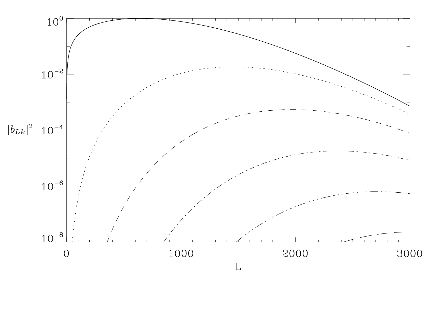
6.2 Using the noise power to set in a temperature only experiment
From the above demonstration, it appears that only a small number of terms in the harmonic expansion of the beam need to be retained in order to capture the global features of the beam response including the effects of asymmetry.
However, to be truly confident that the truncated expansion is an accurate enough representation of the beam, one would ideally choose the value of such that the any residual error from mis-representing the beam is smaller (to some tolerance level) than the statistical error in an experiment. For a particular asymmetric expansion term the leading order contribution to is , where . Therefore we can say that the asymmetric term should be included if
| (51) |
where is a tolerance level to which we require our systematic errors to be below the statistical error. A reasonable choice may be , to ensure that the systematic error is 10% of the noise statistical error. is the standard deviation of the noise power, see equation (31), which is the dominating source of statistical error at high . The term is the mode of the angle coverage quality of the scan strategy defined as
| (52) |
where denotes an average over all pixels on the sky, is the number of hits a pixel receives and the sum over the index is over all observations of a particular pixel. The lower the value of , the better the scan strategy is at removing the bias created by the beam asymmetry due to the azimuthal mode.
The rule of thumb in equation (51) becomes problematic when the sky coverage is small and in the presence of a highly asymmetric beam due to coupling between asymmetric terms of different . This coupling is suppressed in the all-sky case because the cross spectra are small for , which in turn means the coupling matrix is small.
However in the case where the power in the mask extends to high these cross spectra terms can become significant. This results in a significant contribution to the operator by a term of the form , where . This additional contribution could potentially be larger than the term if .
7 Testing the pseudo- on Simulations
In this section, we demonstrate the implementation of the pseudo- technique developed in Section 3 on numerical simulations of two representative types of CMB experiment – a generic balloon-borne experiment and a future satellite mission. Note that we test the performance of the algorithm in the temperature-only case. The implementation of our technique for polarization experiments will be presented in a future paper. For a temperature-only analysis, the coupling is reduced to
| (53) | |||||
| (54) |
The main stages of the simulation pipeline are as follows:
- 1.
We use the HEALPix package to create simulations of the CMB temperature field based on the theoretical CMB power spectrum for the concordance CDM cosmological model.
- 2.
We then create a TOD by convolving the CMB with the telescope beam in the appropriate orientation given the scan strategy.
- 3.
We then calculate the using equation (16).
- 4.
The coupling operator is calculated using the expression in equation (54).
- 5.
With the operator calculated, we then invert it to recover an estimate of the full-sky and beam-deconvolved power spectrum.
Note that we use two different convolution codes for the two classes of experiment that we simulate. For the balloon-like test we calculate each element of the TOD using equation (10). The HEALPix ROTATE_ALMS routine operates on the beam multipole coefficients. This function uses the Wigner D-matrices to rotate the beam coefficients by a set of Euler angles given on input. The TOD element can then be calculated using,
| (55) |
where is the multipole expansion of the beam when it has been rotated through the Euler angles . In this way the whole TOD can be created. While this is accurate and simple it would be impossible to use this approach in the satellite-like experiment as the number of TOD elements and the required would make it computationally infeasible. To create the simulated TOD in the satellite-like case, we use a method similar to the FEBeCoP approach (Mitra et al., 2011) except that do not calculate the effective beams but rather we produce the individual TOD elements. The convolution is simplified by describing the beam in pixel space and we only calculate the value of the beam on a set of neighbouring pixels centred around the pointing centre of the beam. We use pixels within of the centre of the beam (see equation 50) to describe the beam over this localised region of sky.
A second technical challenge was to obtain the Wigner D-matrix transforms of the TOD and the window function. We achieved this by implementing equations (13) and (14) using the expression for the Wigner D-matrix in terms of spin weighted spherical harmonics (equation 17). First, the integral over was performed using a simple Newton-Cotes numerical integration method. The HEALPix routine MAP2ALM_SPIN was then used to perform the integrals over and .
7.1 Balloon-like experiment
For our first test we use the simulated LSPE beam shown in Fig. 1 with a modification. We greatly amplify the size of the asymmetry in order to produce a more stringent test of the asymmetry correction algorithm. The spherical harmonic decomposition of this exaggerated beam is related to the original LSPE decomposition by
| (56) |
We use the planned scan strategy for LSPE but we stress that we have not included the effects of the half-wave plate (HWP) that LSPE will use. The LSPE experiment will incorporate a HWP in front of the optics which will be used to increase the polarization angle coverage of the experiment. However, for the purposes of this demonstration where we consider a temperature-only experiment, we have ignored the (advantageous) effects of the HWP. LSPE will be launched at a latitude of 780 North and will follow a jet stream around the globe staying at roughly the same latitude. The payload will spin at 3 rpm and the telescope will perform constant allevation scans with regular (§daily) steps in elevation (The LSPE collaboration et al., 2012).
We created a set of TOD following the above procedure including white noise. The LSPE scan strategy covers of the sky and so provides a test of the algorithm’s ability to account for a cut sky in addition to the effects of beam asymmetry. Fig. 3 shows an example of a simple binned map created from one of our simulations. This figure also shows the hit map of the scan strategy, the coverage quality defined in Section 6.2 and the weighting function that we use to apodise the hit map. We include an (unrealistically high) noise level of mK-arcmin in our simulations in order to test the removal of noise bias from the recovered power spectrum.
 |
 |
 |
 |
The for 1000 realisations were computed according to equation (53) and the coupling operator was calculated using equation (54). In order to invert the coupling matrix we needed to bin the and the coupling operator, as in Hivon et al. (2002). This binning ensures that the matrix is invertible and that the resulting data points are uncorrelated. Here we use a bin size of . A correction for noise bias was also implemented following the procedure outlined in Section 3.4. Fig. 4 shows the mean power spectrum recovered from the simulations in comparison to the input spectrum. In this figure, we also plot the mean power spectrum recovered when the beam was assumed to be axisymmetric, by including only the term on the pseudo-. This figure clearly demonstrates that our algorithm can successfully recover the power spectrum in a situation where the axisymmetric approximation clearly fails. The power spectrum obtained in the case where the noise in the TOD was ignored is also shown demonstrating the ability of our algorithm to successfully correct for noise bias.

7.2 Satellite-like experiment
The second test that we perform is using a satellite-like scan strategy. For this test, we use a beam described be equation (50) with arcmin corresponding to a FWHM of 7 arcmin and . The scan strategy used is similar to that proposed for the Experimental Probe of Inflationary Cosmology (EPIC, Bock et al. 2009). In Fig. 5 we show the hit map, the quality (equation 52) and the weighting function that we have used to mask the galaxy and extragalactic sources. We use the same mask as was used by the Planck collaboration (Planck Collaboration et al., 2013b) for their power spectrum analysis. The weighting function also apodises the hit map. Note that the EPIC scan strategy was designed to improve the coverage quality defined in Section 6.2. This choice of scan strategy will therefore be effective in mitigating beam asymmetries even in the absence of a dedicated correction algorithm. We therefore expect the bias, in the absence of a dedicated correction, to be much smaller than seen in the previous section (although it will still be non-zero). The mean recovered power spectra using are shown in the top panel of Fig. 6. The lower panel of this figure shows the fractional residual bias in the power spectrum recovery and demonstrates an unbiased result to high- when is used. These simulations included white noise such that the error on the map is equivalent to K-arcmin. We can see that even with a scan strategy designed to optimise crossing angles and thereby reduce the asymmetry bias, there remains a bias at the level of when the axisymmetric approximation is made.
 |
 |
 |
The importance of this test is two-fold. It demonstrates that the algorithm can deal with a more conventional elliptical Gaussian beam and also that it can be extended to high-. The coupling operator was calculated in 9 hrs on one 2.26 GHz processor to . We calculated the coupling operator to a much higher than the maximum multipole of interest to ensure that we did not miss any effects from the aliasing of power from higher multipoles.
 |
8 Testing the map-making algorithm on Simulations
We test the map-making algorithm described in Section 5 in two ways. First, we use the algorithm on multiple realisations of the same simulated experiment as described in Section 7.2 to show that the algorithm can correctly remove the asymmetry bias on the temperature power spectrum. The second test is performed on a single noise-free full sky simulation of the satellite experiment. We use this latter simulation to test if the algorithm can successfully remove the asymmetry bias directly from the temperature and polarisation maps. We do not include a CMB polarisation signal in our TOD and so a successful asymmetry correction algorithm should recover a zero polarisation signal.
8.1 Removing the asymmetry bias on the temperature power spectrum
As in Section 7.2, we create 48 TOD realisations using the satellite-like scan strategy, and using an elliptical Gaussian beam with arcmin and (see equation 50). As before, the TOD included white noise equivalent to a map noise level of K arcmin.
From the simulated TOD, we then compute both a simple binned map and a map constructed using the algorithm presented in Section 5 with . We then apply the same galactic and point source mask to these maps as used in Section 7.2. A standard pseudo- analysis (Hivon et al., 2002) is then applied in order to recover the power spectrum. The recovered power spectrum is then deconvolved by dividing by the beam window function , which is the axisymmetric component of the input beam. Fig. 7 shows the recovered power spectrum for the binned map and for the asymmetry cleaned map obtained using the new map-making algorithm of Section 5. The asymmetry bias has clearly been removed successfully. Note that the removal of the asymmetry bias comes at the cost of a modest inflation of the power spectrum error-bars which have increased by . This increased error is modest compared to the systematic bias that has been removed.
 |
8.2 Removing the asymmetry bias on the temperature and polarisation maps
Here we present a demonstration of how the map-making algorithm can be used to remove the asymmetry bias on both the temperature and polarisation maps.
To estimate the temperature map, the algorithm of Section 5 extracts only the spin-0 components of the TOD. This quantity contains the temperature of the CMB smoothed with the axisymmetric component of the beam. To demonstrate this we simulate a noise free TOD using the elliptical Gaussian and the satellite-like scan strategy. We plot the CMB used in the simulation smoothed with the axisymmetric component of the beam in the top panel of Fig. 8. The other three panels in this figure show the absolute error between this isotropically smoothed map and a simple binned map (second panel); and between the isotropically smoothed map and maps produced using the map-making algorithm with and (lower two panels). The reduction in the bias due to beam asymmetry as is increased is clearly demonstrated by this figure.
We also tested the ability of the map-making algorithm to remove the leakage from temperature to polarisation due to the asymmetry of the beam. We performed this test using the approach described in Section 5.2 which makes use of a previously estimated temperature map obtained with the method described in Section 5.1 with . In our simulation we have not included an input polarisation signal so the expected power in the polarisation maps will be zero in the absence of systematics. As described in Section 4, the temperature to polarization leakage could contaminate either the -mode or the -mode power spectrum depending on the relative orientation between the beam ellipticity and the polarisation response of the detector.
In Fig. 9 we plot the power of the leaked temperature to polarisation signal and the power in the polarization maps after this leakage has been removed using the appproach described in Section 5.2. The power in the cleaned polarisation map has been successfully reduced by 4 orders of magnitude compared to the uncleaned map.
 |
 |
 |
 |

9 Discussion
We have developed two separate techniques to remove asymmetry bias in CMB experiments. The first is a pseudo- method that corrects for the asymmetry bias on the temperature and polarisation power spectra. There is no assumption on the scan strategy and only a modest approximation to the beam is required. The analysis is similar to the MASTER algorithm (Hivon et al., 2002) and its extension to polarisation (Brown, Castro, & Taylor, 2005). However we include additional contributions to the coupling operator that corrects for the contaminating effects of the beam asymmetry. We note that this algorithm can only be applied to experiments that can directly measure the and Stokes parameters in the timeline, e.g. a differencing experiment with both instrument- and instrument- detectors on its focal plane. This is due to the fact that we make no attempt to make a map and so we must have measurements of the Stokes parameters in the telescope’s frame of reference. At present the formalism assumes the four beams required for such a differencing experiment are the same. In future work we will relax this assumption.
Using this formalism we also examined the inter-spectra coupling resulting from the beam asymmetry. As an example, we investigated the coupling between temperature and B-mode power in the presence of an ideal scan strategy. In doing so we showed that the temperature power will be coupled to the B-mode power if the beam asymmetry is at an angle to the polarisation sensitivity direction of the detector. This result is in agreement with previous work (Shimon et al., 2008).
The coupling operator in equation (24) allows us to calculate the contribution to each pseudo- from the sky power, due to both the mask and beam asymmetry. By inverting this operator we can, therefore, calculate an unbiased estimate for the CMB power spectra. To calculate the operator we must cap the azimuthal dependence of the beam, . We demonstrated in Section 6, and in Figs. 1 and 2, that a simulated beam from a multi-moded horn, and an elliptical Gaussian, equation (50), are both well described by only a few azimuthal modes. This property allows us to remove to a high degree of accuracy the bias due to the beam asymmetry for any given scan strategy.
We then went on to implement this algorithm in the temperature only case for two simulated experimental set-ups: a balloon-like experiment and a satellite-like experiment. We showed that we could successfully recover the input power spectrum, when the TOD was created using a highly asymmetric beam in the presence of both a severe sky-cut and instrument noise. These tests showed that the algorithm can deal comfortably with beams that have much higher levels of asymmetry than that typically found in real CMB experiments, and using two completely different and realistic scan strategies. The scan strategies investigated include the proposed scanning mode for the forthcoming balloon-borne LSPE experiment (The LSPE collaboration et al., 2012), and a scan strategy optimized for a possible future CMB polarization satellite mission (Bock et al., 2009).
The second technique that we propose for removing beam asymmetry bias is a new map-making algorithm. The map-making algorithm produces temperature and polarisation maps of the CMB that are smoothed with only the axisymmetric component of the beam. It achieves this by separating out the different spin components of the detected signal using equation (42). This allows us to obtain unbiased estimates for the spin-0 and spin-2 components of the signal which correspond to the temperature and polarisation of the pixel. The temperature map estimated using this technique will be clean of systematics due to the asymmetry of the beam. However, the polarisation map will still contain a temperature to polarisation leakage term due to the azimuthal mode of the beam. This contaminating signal can effectively be removed by calculating the leakage from the estimated temperature map and the known beam response as described in Section 5.2.
Removing the effects of beam asymmetry at the map level is preferable to removing it using the pseudo- method. There are three main reasons for this. Firstly there will be no aliasing between spectra. By removing the inter-spectra leakage at the power spectrum level we will increase the statistical error on the recovered power spectra by a factor proportional to the amplitude of the leaked spectra. A more optimal estimate of the true power spectrum can therefore be obtained if we can remove the leakage in the map domain. Secondly, the map-making algorithm can be applied before foregrounds are removed, allowing the application of traditional foreground removal techniques on the beam asymmetry-cleaned maps. Thirdly, the cleaned maps can subsequently be used for other science applications beyond the power spectrum such as CMB lensing, non-Gaussianity studies and foreground science. Note error propagation from uncertainty in the beam shape may be more complicated. We propose that an experiment should Monte-Carlo over uncertainties in the beam to be able to fully understand the errors on the map and therefore the science.
The map-making algorithm requires a scan strategy to cross a pixel at multiple orientations. If this is not the case, the matrix , defined in equation (41), is not invertible. In such cases, the map-making method cannot be applied (although the pseudo-Cℓ approach could still be used). We note that, as an alternative to a highly redundant scan strategy, the required polarisation angle coverage could also be provided through the use of an appropriately positioned HWP, as is the case in the LSPE experiment (The LSPE collaboration et al., 2012).
In Section 8 we showed that we could use the map-making algorithm to correctly recover an input temperature power spectrum free of asymmetry bias for the same simulated satellite-like experiment as was used to test the pseudo- technique. In doing this we found that the noise level in the recovered power spectrum increased by compared to that recovered from a simply binned map. We also demonstrated that we could successfully correct the temperature and polarisation signal for the effects of beam asymmetry at the map level. To demonstrate this, we simulated a satellite-like experiment free of noise and we computed the temperature and polarisation maps using the algorithm described in Section 5. For the case of we showed that the residual error between the resulting estimated temperature map and the input temperature map smoothed with the axisymmetric component of the beam was comparable to the numerical error in the convolution code. Finally, we have also demonstrated that this method could be very powerful for correcting for temperature to polarization leakage due to beam asymmetries. This ability, which is demonstrated in Fig. 9, could prove extremely useful for controlling systematics due to beam asymmetries in future precision CMB -mode polarization experiments.
Acknowledgments
CGRW acknowledges the award of a STFC quota studentship. MLB is grateful to the European Research Council for support through the award of an ERC Starting Independent Researcher Grant (EC FP7 grant number 280127). MLB also thanks the STFC for the award of Advanced and Halliday fellowships (grant number ST/I005129/1). We also thank Bruno Maffei and the LSPE collaboration for helpful discussions. Some of the results in this paper have been derived using the HEALPix (Górski et al., 2005) package.
References
- Bischoff & BICEP Collaboration (2013) Bischoff C., BICEP Collaboration, 2013, IAUS, 288, 61
- Bock et al. (2009) Bock J., et al., 2009, arXiv, arXiv:0906.1188
- Brown, Castro, & Taylor (2005) Brown M. L., Castro P. G., Taylor A. N., 2005, MNRAS, 360, 1262
- Brown et al. (2009) Brown M. L., et al., 2009, ApJ, 705, 978
- Buder & BICEP Collaboration (2013) Buder I., BICEP Collaboration, 2013, AAS, 222, #103.01
- Challinor (2013) Challinor A., 2013, IAUS, 288, 42
- Challinor et al. (2000) Challinor A., Fosalba P., Mortlock D., Ashdown M., Wandelt B., Górski K., 2000, PhRvD, 62, 123002
- Chiang et al. (2010) Chiang, H. C., Ade, P. A. R., Barkats, D., et al. 2010, ApJ, 711, 1123
- Goldberg et al. (1967) Goldberg J. N., Macfarlane A. J., Newman E. T., Rohrlich F., Sudarshan E. C. G., 1967, JMP, 8, 2155
- Górski et al. (2005) Górski, K. M., Hivon, E., Banday, A. J., et al. 2005, ApJ, 622, 759
- Hanson et al. (2013) Hanson, D., Hoover, S., Crites, A., et al. 2013, Physical Review Letters, 111, 141301
- Hanson, Lewis, & Challinor (2010) Hanson D., Lewis A., Challinor A., 2010, PhRvD, 81, 103003
- Hivon et al. (2002) Hivon E., Górski K. M., Netterfield C. B., Crill B. P., Prunet S., Hansen F., 2002, ApJ, 567, 2
- Keihänen & Reinecke (2012) Keihänen E., Reinecke M., 2012, A&A, 548, A110
- Kovac et al. (2002) Kovac, J. M., Leitch, E. M., Pryke, C., et al. 2002, Nature, 420, 772
- The LSPE collaboration et al. (2012) The LSPE collaboration, et al., 2012, arXiv, arXiv:1208.0281
- Mitra et al. (2011) Mitra S., Rocha G., Górski K. M., Huffenberger K. M., Eriksen H. K., Ashdown M. A. J., Lawrence C. R., 2011, ApJS, 193, 5
- Montroy et al. (2006) Montroy, T. E., Ade, P. A. R., Bock, J. J., et al. 2006, ApJ, 647, 813
- O’Dea, Challinor, & Johnson (2007) O’Dea D., Challinor A., Johnson B. R., 2007, MNRAS, 376, 1767
- Planck Collaboration et al. (2013a) Planck Collaboration, et al., 2013a, arXiv, arXiv:1303.5062
- Planck Collaboration et al. (2013b) Planck Collaboration, et al., 2013b, arXiv, arXiv:1303.5068
- Planck Collaboration et al. (2013c) Planck Collaboration, et al., 2013c, arXiv, arXiv:1303.5076
- Polarbear Collaboration et al. (2013) Polarbear Collaboration, et al., 2013, arXiv, arXiv:1312.6646
- QUIET Collaboration et al. (2012) QUIET Collaboration, et al., 2012, arXiv, arXiv:1207.5562
- Ramamonjisoa et al. (2013) Ramamonjisoa F. A., Ray S., Mitra S., Souradeep T., 2013, arXiv, arXiv:1309.4784
- Readhead et al. (2004) Readhead, A. C. S., Myers, S. T., Pearson, T. J., et al. 2004, Science, 306, 836
- Shimon et al. (2008) Shimon M., Keating B., Ponthieu N., Hivon E., 2008, PhRvD, 77, 083003
- Souradeep et al. (2006) Souradeep T., Mitra S., Sengupta A., Ray S., Saha R., 2006, NewAR, 50, 1030
- Wandelt & Górski (2001) Wandelt B. D., Górski K. M., 2001, PhRvD, 63, 123002
- Varshalovich et al. (1988) Varshalovich, D., Moskalev, A., Khersonskiĭ, V., 1988. Quantum theory of angular momentum. World Scientific Publishing Co. Inc.
Appendix A Relationship between our pseudo- and the standard pseudo-
Here we show that the pseudo- expression derived in Section 3 reduces to a rewriting of the standard polarised pseudo- presented in Brown, Castro, & Taylor (2005), in the case where the beam is axisymmetric and where the experiment has both instrument- and instrument- detectors. We begin by looking at the coupling kernel,
| (57) |
We use the weighting function to apodise the hit map and apply a galactic mask. While, in general, it can be a function of , and , in practice, it is sufficient for it to be a function of just and . The function will be discretised. It should be chosen such that for a given pixel ranges from 0 to 1 and acts as the standard window function in the pseudo-. The requirement that the experiment has both an instrument- and - detector means that for every orientation of the telescope we have 4 detections of the sky each at , where j=0,1,2,3. A consequence of this arrangement of detectors is that
| (59) |
Therefore if . We can now examine the Wigner decomposition of the time stream, in particular the components, as these will contain information on the temperature and polarisation of the CMB. We also assume the beam to be axisymmetric and have a zero cross polar response, so that for . We make this assumption in order to make the connection with the standard pseudo- approach. Applying these constraints to equation (18) we get,
| (60) | |||||
| (61) |
Using these expressions, we can show that - and -mode-like decompositions (equations 33 & 34) of the TOD in this experiment will be,
| (62) |
where we have defined,
| (63) | |||||
| (64) |
Comparing the expressions of equation (62) with equation (10) of Brown, Castro, & Taylor (2005) shows that the - and -mode-like decompositions of the TOD defined in equations (33) & (34) have a similar form to the - and -mode decompositions of a polarisation map used in the standard pseudo- technique. They are similar in the sense that they are both the sky polarisation smoothed with the beam, and then convolved with a window function. They differ only in normalisation factors. As the decompositions are similar, the pseudo- constructed from them will also be similar.
Appendix B Product of two coupling kernels
We require the product of two coupling kernels. In order to calculate this, we start from the definition the Kernel
| (65) | ||||
| (66) | ||||
where the second equality comes from an identity found in Varshalovich et al. (1988). We can now evaluate the product summed over certain indices , and
| (71) | ||||
The Wigner 3 orthogonality relation is
which enables the sum over and to be performed and evaluating the Kronecker gives
We can simplify this further by defining the window correlation matrix . Also we can use the selection rule in the 3 symbols that states that the sum of the bottom row must be equal to zero for the symbol to be non-zero. This gives us
Appendix C Symmetries in
The symmetries in the matrix are important to reduce the computation time. First we look at swapping the indices and along with and :
| (104) |
where we have used the definition of window correlation matrix to say that . Now we look at the reversing the sign of all . This implies that
| (105) |
Now we can show symmetry in the matrix is given by
| (114) |
where in the second equality we have used the relation
Appendix D Explicit form of the coupling operator
In section 3.3 we use the coupling operator . Here we explicitly write it in terms of the sub operators
Appendix E Relations between and
The following matrix operation allows conversion from to ,
The matrix is not square, this does not imply that there is more information in the right than the left. There are the same number of degrees of freedom on both sides this is because .