The general property of dynamical quintessence field
Abstract
We discuss the general dynamical behaviors of quintessence field, in particular, the general conditions for tracking and thawing solutions are discussed. We explain what the tracking solutions mean and in what sense the results depend on the initial conditions. Based on the definition of tracking solution, we give a simple explanation on the existence of a general relation between and which is independent of the initial conditions for the tracking solution. A more general tracker theorem which requires large initial values of the roll parameter is then proposed. To get thawing solutions, the initial value of the roll parameter needs to be small. The power-law and pseudo-Nambu Goldstone boson potentials are used to discuss the tracking and thawing solutions. A more general relation is derived for the thawing solutions. Based on the asymptotical behavior of the relation, the flow parameter is used to give an upper limit on for the thawing solutions. If we use the observational constraint and , then we require for the inverse power-law potential with tracking solutions and the initial value of the roll parameter for the potentials with the thawing solutions.
pacs
95.36.+x, 98.80.-kI Introduction
The recent cosmic acceleration observed by type Ia supernova data [1, *hzsst98, *scpsn98] was usually explained by introducing a dynamical scalar field called quintessence [4, *wetterich88, 6, 7]. More general dynamical scalar field models such as phantom [8], quintom [9, *Feng:2004ff, *Guo:2004fq], tachyon [12, *Sen:2002nu, *Padmanabhan:2002cp] and k-essence [15] were also proposed. For a recent review of dark energy, please see Ref. [16, *copelandde, *Nojiri:2006ri, *Padmanabhan:2007xy, *limiaode, *Nojiri:2010wj, *Bamba:2012cp].
For a dynamical scalar field with the potential in the flat Friedmann-Lemaître-Robertson-Walker universe with the metric , its energy density and pressure are and , where . The scalar field rolls down a very shallow potential while its equation of state approaches and it starts to dominate the Universe recently. Because the scalar field catches up the background only recently and the current value of its equation of state parameter is around , does not change too much in the redshift range for most scalar fields, so the time variation of is bounded for the thawing and freezing models [23, 24, 25, 26, 27, *chiba06a, 29, 30, 31, 32]. In general, the evolution of scalar field depends on the initial conditions. However, the attractor solutions and the tracking solutions are independent of the initial conditions [33, *Ferreira:1997hj, 35, 36, 37, 38, 39, 40, 41, 42, *Johri:2001wm, 44, 45, 46, 47, 48, 49, 50, 51, 52]. In particular, the tracker field tracks below the background density for most of the history of the Universe until it starts to dominate recently for a wide range of initial conditions, and there exists a relation between and the fractional energy density today, where the Hubble parameter . There also exists a general relation for the thawing solutions which is well approximated by some analytical expressions [53, 54, 55, 56, 57, 58, 59, 60, 61, 62, 63]. In this Letter, we will discuss the general dynamics such as the relation and the bound on of the tracking and thawing fields. We use the power-law potential and the pseudo-Nambu Goldstone boson (PNGB) potential [64, 65, 66, 67, 68] as examples to illustrate the general dynamical behaviors of tracking and thawing fields.
If the Universe is filled with the quintessence field and the background matter with the equation of state , where [69] is the scale factor at the matter-radiation equality, then in terms of the dimensionless variables,
| (1) |
the cosmological equations are
| (2) | |||
| (3) | |||
| (4) |
The fractional energy density and the equation of state of the scalar field are
| (5) |
Using the fractional energy density and the parameter , Eqs. (2)-(4) become
| (6) | |||
| (7) | |||
| (8) |
From Eq. (7), we get a lower limit . If the tracker parameter can be expressed as a function of the roll parameter , then the above system (6)-(8) becomes an autonomous system. In this case, we have additional critical point and which is absent in the system (2)-(4), where the subscript means the critical point. At the point and , the transformation from to is singular, so we get different critical points. Only when , the point and is the critical point of the system (2)-(4). For the exponential potential, the point and is not a critical point for the system (2)-(4) and the critical point and for the system (6)-(8) is not a stable point.
If we use the flow parameter [30], then Eq. (7) can be written as
| (9) |
To understand the general dynamics of the quintessence, it is useful to use the function [30, 60],
| (10) |
For the thawing solution, the quintessence field rolls down the potential very slowly, and is almost a constant, so at early time when and [60].
II Tracker solution
The energy density of the tracker field tracks below the background density for most of the history of the Universe, it starts to dominate the energy density only recently and then drives the cosmic acceleration. The tracker fields have attractor-like solutions in the sense that they rapidly converge to a common cosmic evolutionary track of and for a very wide range of initial conditions, so the tracking solutions are extremely insensitive to the initial conditions [7, 37]. Furthermore, an important relation between and today was found for the tracker field. When the tracker field enters the tracking solution, it satisfies the tracker condition [37]
| (11) |
thus this condition is the initial condition of tracking solution. In other words, the initial condition for the tracking solution reads . From Eq. (7), we see that when the tracker condition is satisfied, so it is possible that stops varying. On the other hand, the quintessence field satisfies the tracker equation [37, 44]
| (12) |
where and . For the tracking solution, is nearly constant, so , and we get
| (13) |
If when the tracker condition (11) is satisfied, then
| (14) |
and are approximately constants if the tracker parameter is nearly constant, increases with time and decreases with time. For the tracker field, is not negligible, so . In fact, is a constant for the exponential potential when the attractor is reached.
If is not small or the tracker parameter changes rapidly when the tracker condition (11) is satisfied, then won’t keep to be a time independent constant and it decreases with time while increases to 1, so the scalar field does not track the background and Eq. (14) does not hold when the tracker condition (11) is satisfied, but the scalar field has the the freezing behavior with asymptotically. Therefore, both the tracker condition (11) and Eq. (14) will be violated when is not negligible or changes rapidly, and keeps decreasing.
For the tracker field, the tracking solution at late times has the property that and , so should decrease with time while increases with time. When reaches the background value , and decreases to the value , then we reach the tracker condition. After that, decreases toward to zero and increases toward 1. From Eq. (7), we know that we should keep in order that , therefore should decrease with time and when . For any quintessence field rolling down its potential, does not increase with time is equivalent to as easily seen from Eq. (8).
For the exponential potential, is a constant and . If is small, then eventually will decrease to be less than , and will quickly increase to be 1. In particular, if , then the system will reach the attractor solution with and . If is big, i.e., , then the attractor solution is . Since the above attractors satisfy the tracker condition (11), so both of them are also tracking solutions. In Fig. 1, we show the phase diagram for the exponential potential with . The original tracking solution found in [37] is independent of the value of which is in contradiction with the results for the exponential potential. The contradiction was then resolved in [44] by deriving the correct tracker equation (12).

With the dynamical Eqs. (6)-(8), we can understand the general dynamical evolution of the tracker field as follows: (a) Initially if is not too small or is large enough so that , where the subscript means the initial value, then will increase toward 2 independent of the initial value of . Once , will decrease. When decreases to be small enough so that , decreases toward and starts to increase once . Even if decreases, it will overtake when , then increases again. Once increases away from zero, we will have and the tracker behavior of will be reached, maybe after several oscillations. If is small, then to satisfy the tracker condition, cannot be too small and may reach very quickly and the tracker solution with nearly constant will not appear. (b) Initially if or is small so that , then decreases toward 0 and starts to increase once independent of the initial value . After that, the dynamics is similar to that in case (a). In this case, even though is small, but it always increases if is small, will reach 1 soon and the tracker solution with nearly constant does not appear. Of course, the current values of , and depend on their initial values. From these analyses, we conclude that if the initial value of is small, then no tracker solution with nearly constant appears because reaches 1 too soon. For small , once reaches 1, the equation for decouples from the dynamical system (6)-(8). Therefore, the solution to Eqs. (7) and (8) gives a relation between and . Since approaches asymptotically, the relation is universal if is a function of in the sense that it does not depend on the initial conditions, therefore the relation is also universal when .
For the tracking solution, the conditions (11) and (14) are the initial conditions, so for the same initial value of at the start of the tracking solution, the trajectories of , an will be the same, that is why we have the same trajectory for the tracking solution independent of the initial conditions. However, the exact values of and at a moment (for instance, at the present) still depend on the initial conditions. We refer the tracking solutions as those solutions which have a common trajectory for a wide range of initial conditions, technically, the tracking solutions satisfy the two conditions (11) and (14) initially.
In [31], the author rephrased the tracker theorem as: the tracker property appears for any scalar field model in which the roll parameter is capable of taking on large initial values in the early Universe. If decreases with time, then is capable of taking on large initial values in the early Universe. However, for the power-law potential with , the roll parameter can be large if we start from small , and there is no tracking solution. Furthermore, it is not clear how large the initial value should be. Therefore, we propose the tracker theorem as: the tracker behavior appears for any quintessence field in which the roll parameter does not increase with time and the initial value of should be big enough so that is still negligible when the tracker condition (11) is satisfied. The new definition of the tracking solution and the tracker theorem proposed here are parts of the main results of this Letter.
III Power-law potential
In this section, we use the power-law potential as an example to explicitly show the analyses presented in the previous section. Here we focus on the tracking and thawing behaviors and the bound on . For the power-law potential with the energy scale and the Planck mass , the tracker parameter , so the dynamical system becomes an autonomous system. The dynamical analysis of the system (2)-(4) with was carried out in [49]. The dynamical system (2)-(4) has the following critical points: , with arbitrary, and . Only the critical point can be stable if . For the inverse power-law potential, , so the critical point which corresponds to the solution and is a stable point. From this analysis, we know that will decrease to zero for the tracking solution.
III.1 Tracking solution
If we use the dynamical system (6)-(8), the critical points are: , or with arbitrary ; and with arbitrary ; and . The critical point is a stable point. For the critical point , the linear approximation of the system (6)-(8) is
| (15) | |||
| (16) | |||
| (17) |
One of the eigenvalues is 0. To analyze the stability of the system, we need to understand the stability of equation (8) for the critical point by using the center manifold theorem [70]. So we need to solve the following equation [70]
| (18) |
Let , up to the order of , we get . Substituting and into Eq. (8), we get
| (19) |
The system is stable if , so the critical point of the dynamical system (6)-(8) is a stable point for the inverse power-law potential. From the above analysis, we see that asymptotically to the leading order, so this stable critical point corresponds to the late time tracking solution. In other words, the flow parameter starts with the value and approaches the value asymptotically for the tracking solution. The function starts with and increases to asymptotically.
Because the dynamical system (6)-(8) is hard to solve numerically if is too large, we choose to solve the dynamical system (2)-(4) numerically for the inverse power-law potential to illustrate the tracking behavior and the results are shown in Fig. 2. As seen from Fig. 2, the general dynamics of the tracker field follows our discussion in the previous section, and exhibits oscillatory behaviors before the scalar field reaches the tracking solution. For small (for this case, ), the tracking solution with constant does not appear because reaches in a short time. Even though the general relation was not followed as shown by the dotted lines in Fig. 3, the same and relations are still followed for those solutions with small when approaches . For large , the tracking behavior is realized easily. But to get the observationally allowed (the subscript means the current value), we need to adjust the initial values of , and . For the example shown in Fig. 2, we choose and so that . We also show the relation between and for the tracking solutions with different initial conditions in Fig. 3. Not only the relation between and exists, but also the same relation follows for and at any moment after it reaches the tracking solution. This is one of the main results obtained in this Letter.
 |
 |
 |
 |
As we discussed in the previous section, the - trajectory is independent of the initial conditions, so the - relation is the same as the general - relation for the tracking solution because of the tracker condition, although the values of and depend on the initial conditions. Therefore, we generalize the common trajectory found in [7, 37] to the common trajectory for the tracking solutions even though evolves differently when the tracker field starts to dominate the Universe. The trajectory can be obtained by solving the dynamical system (6)-(8) with the initial conditions (11) and (14). A general - relation was proposed in [55] for slow-roll freezing quintessence by assuming constant as
| (20) |
Apparently, this relation cannot be applied for the tracking behavior because when and when if . The reason why the above relation does not work is that is not a constant for the tracking solution as shown in Fig. 3. When is small, a linear approximation for the relation was found in [45, 71]. We find that the general relation for can be fitted by the following function
| (21) |
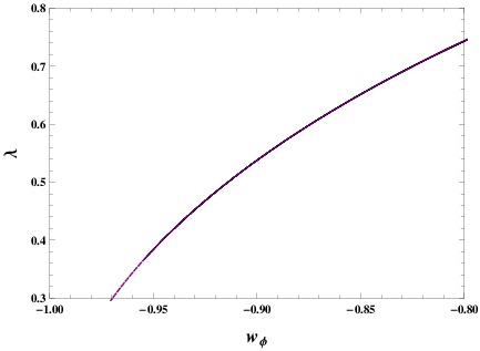
It is obvious that does not differ much from the initial value (14), so is small. To see how small it is, we show the trajectory for different in Fig. 4. The upper limit [23] is also shown in Fig. 4. Our results show that the upper limit is violated. As we discussed above, as , and , so we expect the violation of the upper limit . The other problem is the observational constraints on the values of and . Since and follow a universal relation which is independent of the initial conditions and the energy scale of the potential, we can use the observational data to constrain the form of tracker potential. For the power-law potential , the observational constraints can be satisfied by choosing small as shown in Fig. 4. If we choose the observational constraints and [72, 73], then we require .
 |
 |
III.2 Thawing solution
For the inverse power-law potential, if is small, then decreases to as seen from Eq. (7). If we also fine-tune the initial value of (for , is around at ), then stays at the value and starts to increase recently, we get the thawing behavior. From Eq. (8), it is easy to see that will keep to be a constant when . Combining Eqs. (6) and (7), we get
| (22) |
Taking the approximation , then Eq. (22) can be approximated as
| (23) |
The solution to the above Eq. (23) with constant is
| (24) |
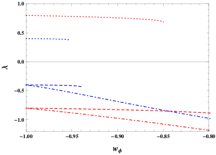
where is the hypergeometric function. This approximation breaks down when . As and , , so the flow parameter and which is consistent with the result found in [60] with different argument. If starts to increase during the matter domination, and , we recover the familiar relation (20) with . We show the evolutions of , and in Fig. 5, and the and relations are shown in Fig. 6 with dotted lines for the inverse power-law potential with . We choose two different initial values of and . The thawing solution was kept up to for and for . When the scalar field takes the thawing solution, is almost a constant as shown in Fig. 5 and the analytical relation (24) approximates the relation well as shown in Fig. 6. Since , the larger is, the faster changes, so the analytical relation (24) gives better approximation for smaller as shown in Fig. 6.
 |
 |
 |
 |
For the power-law potential with positive , the roll parameter increases with time and there is no asymptotically freezing solution. To get the thawing solution, we need to start with small so that decreases to . If we also fine-tune the initial value of (for , is around at ), then stays at the value and starts to increase recently. We show the evolutions of , and in Fig. 5, the and relations in Fig. 6 by the dashed lines for the power-law potential with . We choose two different initial values of and . When the scalar field takes the thawing solution, is almost a constant as shown in Fig. 5 and the analytical relation (24) approximates the relation well as shown in Fig. 6. Again the analytical relation (24) gives better approximation for smaller as shown in Fig. 6. If we use the observational constraints and , then the analytical relation (20) requires . From the analytical relation (20), we see that as which is not true for the positive power-law potential because keeps increasing and it increases faster and faster once deviate from , this means that the approximation is broken as . On the other hand, as , we get , so the flow parameter initially at the matter domination for the thawing solution and the flow parameter when the quintessence field leaves the thawing solution. Therefore, for the thawing solution, we get an upper limit which is smaller than the upper limit [23], and there is no lower limit on . As shown in Fig. 6, the lower limit [23] does not hold. These two upper bounds are also shown in Fig. 6 and they are satisfied by the thawing solutions. From Eq. (10), we get initially and when the thawing period ends.
IV PNGB potential
In this section, we focus on the approximation (24) and the limit on for the PNGB potential. The PNGB potential was first proposed in the schizon model in which the small PNGB mass is protected by fermionic chiral symmetries [64, 65], meson and the axion are examples of PNGB. In cosmology, the PNGB potential was first introduced as natural inflation [66], and was later found that it also dominates the energy density of the universe at present [67]. In this Letter, we choose the PNGB potential without loss of generality, with the energy scale eV, the tracker parameter and [49], so there is no tracking solution for the PNGB potential. Since is not well defined, the dynamical analysis on the fixed points in [49] is not applicable. The critical points are: , or with arbitrary ; and with arbitrary ; and . In fact, all the critical points are unstable points.
In this model, , the roll parameter changes faster than the power-law potential, so we don’t expect that the analytical expression (24) approximates the as well as that for the power-law potential with the same . To get the thawing solution, we also need to start with small so that quickly reaches the initial thawing value , and we also need to fine-tune the initial value of to be around at . The evolutions of , and are shown in Fig. 5, and the and relations are shown in Fig. 6 with dot-dashed lines. As we expect, does not keep to be nearly constant, the approximation (20) is not good for large and it breaks down when approaches 1.
V Discussion and Conclusions
When the tracking solution is reached, , so is almost a constant and both the tracker condition (11) and Eq. (14) are satisfied. To keep to be a constant, should be small and the tracker parameter should be nearly constant, so the tracker condition (11) requires the roll parameter to be large. Therefore, the tracker parameter and large initial value of the roll parameter are the the necessary conditions for tracking solutions. Based on this analysis, we proposed the tracker theorem. Although the current value of and depend on the initial conditions for the tracking solutions, the trajectory before reaches 1 is independent of the initial conditions and it can be used to exclude models by comparing it with the observational constraints. If we choose the observational constraints and , then we require for the inverse power-law potential . Since the dark energy domination () is the attractor for the inverse power-law potential, the asymptotic behaviors of and are the same and the same asymptotic trajectory is followed by all solutions including the tracking and non-tracking solutions. The flow parameter starts and ends with , the upper bound does not hold and we expect that no such upper bound exists for the freezing models, this will make the distinction between cosmological constant and dynamical tracker fields more difficult.
If the initial value of the roll parameter is small, then quickly decreases to -1 and stays at the value until the roll parameter becomes large, after that starts to increase. This thawing behavior can be achieved for the power-law potential with positive and the the PNGB potential. The thawing behavior can also be achieved for the inverse power-law potential for a period of time if the initial value of the roll parameter is small. In general, we need to fine-tune the initial conditions so that we get the right values of and which are consistent with the observational constraints for the thawing solutions. Because initially, the roll parameter changes very slowly and it can be approximated as a constant, a general relation (24) is then obtained. Based on the asymptotical behavior of the relation, the flow parameter when and during the matter domination, and when the thawing behavior ends, we derive the upper bound and we expect that no lower bound exists for the thawing models, so the distinction between cosmological constant and dynamical thawing models becomes more difficult. If we use the observational constraint and , we find that the initial value of the roll parameter for the potentials with the thawing solutions.
In summary, we find that the same relation not only exists between and , but also exists between and at any time after the tracker field takes the tracking solutions. The relation is independent of the initial conditions and the energy scale of the tracker field, so the observational data can be used to constrain the tracker model by using this relation. Based on the existence of the relation, we generalize the tracking solutions with a common track of to those solutions with a common trajectory and we propose the tracker theorem by using the roll parameter . Both the upper limit for the tracking solutions and the lower limit for the thawing solutions are found to be violated, and we propose a lower upper bound for the thawing solutions.
Acknowledgements.
This work was partially supported by the National Basic Science Program (Project 973) of China under grant No. 2010CB833004, the NNSF of China under grant Nos. 10935013 and 11175270, the Program for New Century Excellent Talents in University under grant No. NCET-12-0205 and the Fundamental Research Funds for the Central Universities under grant No. 2013YQ055.References
- [1] S. Perlmutter et al., Nature 391 (1998) 51.
- [2] A. G. Riess et al., Astron. J. 116 (1998) 1009.
- [3] S. Perlmutter et al., Astrophys. J. 517 (1999) 565.
- [4] B. Ratra and P. Peebles, Phys. Rev. D 37 (1988) 3406.
- [5] C. Wetterich, Nucl. Phys. B 302 (1988) 668.
- [6] R. Caldwell, R. Dave, and P. J. Steinhardt, Phys. Rev. Lett. 80 (1998) 1582.
- [7] I. Zlatev, L.-M. Wang, and P. J. Steinhardt, Phys. Rev. Lett. 82 (1999) 896.
- [8] R. Caldwell, Phys. Lett. B 545 (2002) 23.
- [9] B. Feng, X.-L. Wang, and X.-M. Zhang, Phys. Lett. B 607 (2005) 35.
- [10] B. Feng, M. Li, Y.-S. Piao, and X. Zhang, Phys. Lett. B 634 (2006) 101.
- [11] Z.-K. Guo, Y.-S. Piao, X.-M. Zhang, and Y.-Z. Zhang, Phys. Lett. B 608 (2005) 177.
- [12] A. Sen, JHEP 0207 (2002) 065.
- [13] A. Sen, JHEP 0204 (2002) 048.
- [14] T. Padmanabhan, Phys. Rev. D 66 (2002) 021301.
- [15] C. Armendariz-Picon, V. F. Mukhanov, and P. J. Steinhardt, Phys. Rev. Lett. 85 (2000) 4438.
- [16] V. Sahni and A. A. Starobinsky, Int. J. Mod. Phys. D 9 (2000) 373.
- [17] E. J. Copeland, M. Sami, and S. Tsujikawa, Int. J. Mod. Phys. D. 15 (2006) 1753.
- [18] S. Nojiri and S. D. Odintsov, Int. J. Geom. Meth. Mod. Phys. 4 (2007) 115.
- [19] T. Padmanabhan, Gen. Rel. Grav. 40 (2008) 529.
- [20] M. Li, X.-D. Li, S. Wang, and Y. Wang, Commun. Theor. Phys. 56 (2011) 525.
- [21] S. Nojiri and S. D. Odintsov, Phys. Rept. 505 (2011) 59.
- [22] K. Bamba, S. Capozziello, S. Nojiri, and S. D. Odintsov, Astrophys. Space Sci. 342 (2012) 155.
- [23] R. Caldwell and E. V. Linder, Phys. Rev. Lett. 95 (2005) 141301.
- [24] V. Barger, E. Guarnaccia, and D. Marfatia, Phys. Lett. B 635 (2006) 61.
- [25] R. J. Scherrer, Phys. Rev. D 73 (2006) 043502.
- [26] E. V. Linder, Phys. Rev. D 73 (2006) 063010.
- [27] T. Chiba, Phys. Rev. D 73 (2006) 063501.
- [28] T. Chiba, Phys. Rev. D 80 (2009) 129901(Erratum).
- [29] A. Ali, M. Sami, and A. Sen, Phys. Rev. D 79 (2009) 123501.
- [30] R. N. Cahn, R. de Putter, and E. V. Linder, JCAP 0811 (2008) 015.
- [31] L. A. Urena-Lopez, JCAP 1203 (2012) 035.
- [32] X. Chen and Y. Gong, The limit on for tachyon dark energy, arXiv: 1309.2044, 2013.
- [33] P. G. Ferreira and M. Joyce, Phys. Rev. Lett. 79 (1997) 4740.
- [34] P. G. Ferreira and M. Joyce, Phys. Rev. D 58 (1998) 023503.
- [35] E. J. Copeland, A. R. Liddle, and D. Wands, Phys. Rev. D 57 (1998) 4686.
- [36] A. R. Liddle and R. J. Scherrer, Phys. Rev. D 59 (1999) 023509.
- [37] P. J. Steinhardt, L.-M. Wang, and I. Zlatev, Phys. Rev. D 59 (1999) 123504.
- [38] P. Brax and J. Martin, Phys. Rev. D 61 (2000) 103502.
- [39] L. A. Urena-Lopez and T. Matos, Phys. Rev. D 62 (2000) 081302.
- [40] S. A. Bludman and M. Roos, Phys. Rev. D 65 (2002) 043503.
- [41] S. Dodelson, M. Kaplinghat, and E. Stewart, Phys. Rev. Lett. 85 (2000) 5276.
- [42] V. B. Johri, Phys. Rev. D 63 (2001) 103504.
- [43] V. B. Johri, Class. Quant. Grav. 19 (2002) 5959.
- [44] C. Rubano, P. Scudellaro, E. Piedipalumbo, S. Capozziello, and M. Capone, Phys. Rev. D 69 (2004) 103510.
- [45] C. R. Watson and R. J. Scherrer, Phys. Rev. D 68 (2003) 123524.
- [46] J. Aguirregabiria and R. Lazkoz, Phys. Rev. D 69 (2004) 123502.
- [47] M. Sahlen, A. R. Liddle, and D. Parkinson, Phys. Rev. D 75 (2007) 023502.
- [48] D. Huterer and H. V. Peiris, Phys. Rev. D 75 (2007) 083503.
- [49] W. Fang, Y. Li, K. Zhang, and H.-Q. Lu, Class. Quant. Grav. 26 (2009) 155005.
- [50] M. Szydlowski, O. Hrycyna, and A. Stachowski, Int. J. Geom. Meth. Mod. Phys. 11 (2014) 1460012.
- [51] S. del Campo et al., Phys. Rev. D 88 (2013) 023532.
- [52] N. Roy and N. Banerjee, Gen. Rel. Grav. 46 (2014) 1651.
- [53] R. J. Scherrer and A. Sen, Phys. Rev. D. 77 (2008) 083515.
- [54] R. J. Scherrer and A. Sen, Phys. Rev. D. 78 (2008) 067303.
- [55] S. Dutta and R. J. Scherrer, Phys. Lett. B. 704 (2011) 265.
- [56] R. Crittenden, E. Majerotto, and F. Piazza, Phys. Rev. Lett. 98 (2007) 251301.
- [57] S. Dutta and R. J. Scherrer, Phys. Rev. D 78 (2008) 123525.
- [58] T. Chiba, S. Dutta, and R. J. Scherrer, Phys. Rev. D 80 (2009) 043517.
- [59] G. Gupta, E. N. Saridakis, and A. A. Sen, Phys Rev. D 79 (2009) 123013.
- [60] T. Chiba, Phys. Rev. D 79 (2009) 083517.
- [61] S. Sen, A. Sen, and M. Sami, Phys. Lett. B 686 (2010) 1.
- [62] S. del Campo, V. H. Cardenas, and R. Herrera, Phys. Lett. B 694 (2011) 279.
- [63] Y. Gong and Q. Gao, Eur. Phys. J. C 74 (2014) 2729.
- [64] C. T. Hill and G. G. Ross, Phys. Lett. B 203 (1988) 125.
- [65] C. T. Hill and G. G. Ross, Nucl. Phys. B 311 (1988) 253.
- [66] K. Freese, J. A. Frieman, and A. V. Olinto, Phys. Rev. Lett. 65 (1990) 3233.
- [67] J. A. Frieman, C. T. Hill, A. Stebbins, and I. Waga, Phys. Rev. Lett. 75 (1995) 2077.
- [68] K. Coble, S. Dodelson, and J. A. Frieman, Phys. Rev. D 55 (1997) 1851.
- [69] P. Ade et al., Planck 2013 results. XVI. Cosmological parameters, arXiv: 1303.5076, 2013.
- [70] H. K. Khalil, Nonlinear Systems, Third edition (Prentice Hall, New Jersey, 2002).
- [71] T. Chiba, Phys. Rev. D 81 (2010) 023515.
- [72] Y. Gong, Q. Gao, and Z.-H. Zhu, Mon. Not. Roy. Astron. Soc. 430 (2013) 3142.
- [73] Q. Gao and Y. Gong, The tension on the cosmological parameters from different observational data, arXiv: 1308.5627, 2013.