跳到论文正文
W Papers独立论文阅读器 arXiv:1401.1844 论文正文 计算阅读时间 · 0%
引用这篇论文根据当前论文元数据生成,正式投稿前建议核对。


License: arXiv.org perpetual non-exclusive license
arXiv:1401.1844v4 [hep-ph] 05 May 2015

DESY 14-006 ISSN 0418-9833
January 2014
Two-loop electroweak threshold corrections to the bottom and top Yukawa couplings

Bernd A. Kniehl Affiliation: II. Institut für Theoretische Physik, Universität Hamburg,    Oleg L. Veretin Affiliation: Luruper Chaussee 149, 22761 Hamburg, Germany
Abstract

We study the relationship between the MS¯\overline{\mathrm{MS}} Yukawa coupling and the pole mass for the bottom and top quarks at the two-loop electroweak order 𝒪⁡(α2){\cal O}(\alpha^{2}) in the gaugeless limit of the standard model. We also consider the MS¯\overline{\mathrm{MS}} to pole mass relationships at this order, which include tadpole contributions to ensure the gauge independence of the MS¯\overline{\mathrm{MS}} masses. In order to suppress numerically large tadpole contributions, we propose a redefinition of the running heavy-quark mass in terms of the MS¯\overline{\mathrm{MS}} Yukawa coupling. We also present Δ​r\Delta r in the MS¯\overline{\mathrm{MS}} scheme at 𝒪⁡(α2){\cal O}(\alpha^{2}) in the gaugeless limit. As an aside, we also list the exact two-loop expression for the mass counterterms of the bottom and top quarks.

PACS numbers: 11.10.Gh, 12.15.Ff, 12.15.Lk, 14.65.Fy, 14.65.Ha

1 Introduction

The recent discovery of the Higgs boson [1] was a giant leap in particle physics. It confirmed that the concept of spontaneous symmetry braking in connection with the generation of masses by the Higgs mechanism could be realized in nature. This does not explain, however, the very large spread of the fermion masses and the values of the masses themselves. It is generally believed that some grand unified theories could provide a solution to this fundamental problem. An essential rôle in such analyses is played by the renormalization group (RG) equations, which determine the scale dependencies of the running parameters.

Due to the large values of their masses, the bottom quark and, even more so, the top quark attract great interest. Even disregarding the fact that quark masses require special consideration because quarks do not appear as free particles, one may introduce different parameters to describe the notion of quark mass. The most important definitions are those of the pole mass MM, the running mass m⁡(μ)m(\mu) in the modified minimal-subtraction (MS¯\overline{\rm MS}) scheme, and the running Yukawa coupling y⁡(μ)y(\mu), defined in MS¯\overline{\rm MS} scheme as well. Here, μ\mu is the ’t Hooft mass of dimensional regularization. The relationships between these quantities can be obtained in perturbation theory as series in the strong-coupling constant αs\alpha_{s} and Sommerfeld’s fine-structure constant α\alpha. The terms containing ln⁡μ2\ln\mu^{2} can be obtained using the RG beta functions and anomalous dimensions. In QCD, they have been computed in the three- [2] and four-loop [3] approximations. In the standard model (SM), the corresponding RG functions, known through two loops since Ref. [4], have recently been evaluated at the three-loop level [5].

The other aspect of the problem is the matching between the running parameters and the physical observables. These so-called threshold relationships include not only terms with ln⁡μ2\ln\mu^{2}, but also terms of non-logarithmic type. The relation between the MS¯\overline{\rm MS} mass and the pole mass of a quark was elaborated in QCD at one [6], two [7], and three [8] loops. The two-loop result in the supersymmetric extension of QCD was obtained in Ref. [9]. These corrections can be readily applied also to the Yukawa coupling of a quark. However, the situation becomes more complicated if electroweak corrections are taken into account. In this case, the relation between the MS¯\overline{\rm MS} mass and the MS¯\overline{\rm MS} Yukawa coupling of a fermion becomes nontrivial. The full one-loop corrections to the relationships between the MS¯\overline{\rm MS} Yukawa couplings and the pole masses of the fermions were derived in Ref. [10]. The mixed QCD-electroweak two-loop corrections were evaluated for the top quark in Ref. [11] and for the other fermions in Ref. [12] by using the method of large-mass expansion. In some earlier calculations, the tadpole contributions were omitted in the MS¯\overline{\rm MS} to pole mass relations of fermions, e.g. in the calculation of the electroweak parameter Δ​ρ\Delta\rho in the gaugeless limit in Ref. [13]. Expressed in terms of the top-quark and Higgs-boson pole masses, the result for Δ​ρ\Delta\rho thus obtained is correct, but some intermediate results differ from those in Ref. [11]. This situation was clarified in Ref. [14].

The aim of the present paper is to extend the theoretical knowledge of the relationships between the MS¯\overline{\rm MS} masses and Yukawa couplings and the pole masses of the bottom and top quarks by calculating the two-loop electroweak corrections, at order O⁡(α2)O(\alpha^{2}), in the approximation provided by the gaugeless limit.

This paper is organized as follows. In Sections 2 and 3, we give all the necessary definitions concerning the MS¯\overline{\rm MS} mass and Yukawa coupling, respectively. In Sections 4 and 5, we list analytical results for the bottom and top MS¯\overline{\rm MS} Yukawa couplings, respectively. In Section 6, we present our numerical analysis. In Appendix A, we list two-loop expressions for the electroweak parameter Δ​r¯\Delta\bar{r}, which enters the relationships between the MS¯\overline{\rm MS} masses and Yukawa couplings, both in the gaugeless and heavy-top-quark limits. Appendix B contains the exact two-loop renormalization constants of the bottom- and top-quark masses in the MS¯\overline{\rm MS} scheme. In Appendix C, we present the MS¯\overline{\rm MS} to pole mass relation for the bottom quark in the heavy-top-quark limit.

2 Running mass

The pole mass MM of a particle is determined by definition from the position of the pole of its propagator.11 1 If the particle is unstable, then the pole position has a complex value. In this case, the pole mass is usually taken to be the real part of it. We start from the general form of the inverse fermion propagator,

S−1(p/)=p/−m0−Σ(p/),\displaystyle S^{-1}(p\!\!\!/\penalty)=p\!\!\!/\penalty-m_{0}-\Sigma(p\!\!\!/\penalty)\,, (1)

where pp is the four-momentum and m0m_{0} is the bare mass of the fermion. The self-energy function Σ(p/)\Sigma(p\!\!\!/\penalty) is given by the sum of all one-particle-irreducible Feynman diagrams pertaining to the transition of the fermion to itself and depends on further parameters of the theory, such as masses, couplings, and mixing angles. An important comment should be made here. In the SM with the Higgs mechanism, the inclusion of tadpoles (see Fig. 1) is necessary to render the relationship between the pole and bare masses gauge independent [15]. Thus, we include in Σ(p/)\Sigma(p\!\!\!/\penalty) all Feynman diagrams which are one-particle irreducible with respect to all particles except for the Higgs boson.

In the electroweak theory, the left- and right-handed components of a fermion field propagate differently due to parity violation. On the other hand, we take the Cabibbo-Kobayashi-Maskawa quark mixing matrix to be unity and thus effectively turn off CP violation. In this case, the most general decomposition of Σ(p/)\Sigma(p\!\!\!/\penalty) reads [16]:

Σ(p/)=p/ωLAL(p2)+p/ωRAR(p2)+m0B(p2),\displaystyle\Sigma(p\!\!\!/\penalty)=p\!\!\!/\penalty\,\omega_{L}A_{L}(p^{2})+p\!\!\!/\penalty\,\omega_{R}A_{R}(p^{2})+m_{0}B(p^{2})\,, (2)

where ωL,R=(1∓γ5)/2\omega_{L,R}=(1\mp\gamma_{5})/2 are the projectors on the left- and right-handed spinor components, respectively, and ALA_{L}, ARA_{R}, and BB are dimensionless scalar functions of p2p^{2} depending also on the SM parameters.

In order to invert the matrix in Eq. (1), we first decompose it into its left- and right-handed components. The inverse S(p/)S(p\!\!\!/\penalty) may be found in Eq. (10) of Ref. [16]. The poles of its left- and right-handed components coincide and are given by the solution p2=M2p^{2}=M^{2} of the equation [16]

p2​[1−AL​(p2)]​[1−AR​(p2)]−m02​[1+B⁡(p2)]2=0.\displaystyle p^{2}[1-A_{L}(p^{2})][1-A_{R}(p^{2})]-m_{0}^{2}[1+B(p^{2})]^{2}=0\,. (3)

We can solve Eq. (3) perturbatively by substituting the ansatz

M=m0​(1+X1+X2+…),M=m_{0}(1+X_{1}+X_{2}+\dots), (4)

where XiX_{i} refers to the order ii. Explicitly, through second order, we find

X1\displaystyle X_{1} =\displaystyle= B1+12​AL,1+12​AR,1,\displaystyle B_{1}+\frac{1}{2}A_{L,1}+\frac{1}{2}A_{R,1}\,,
X2\displaystyle X_{2} =\displaystyle= B2+12​AL,2+12​AR,2+X1​(AL,1+AR,1+AL,1′+AR,1′+2​B1′)\displaystyle B_{2}+\frac{1}{2}A_{L,2}+\frac{1}{2}A_{R,2}+X_{1}(A_{L,1}+A_{R,1}+A_{L,1}^{\prime}+A_{R,1}^{\prime}+2B_{1}^{\prime}) (5)
−12​X12−12​AL,1​AR,1+12​B12.\displaystyle-\frac{1}{2}X_{1}^{2}-\frac{1}{2}A_{L,1}A_{R,1}+\frac{1}{2}B_{1}^{2}\,.

In Eq. (5), all functions are to be evaluated at p2=m02p^{2}=m_{0}^{2} and the prime stands for the derivative with respect to p2/m02p^{2}/m_{0}^{2}. The self-energy function in Eq. (2) is gauge dependent and, in general, also infrared divergent. However, the coefficients XiX_{i} in Eq. (4) are manifestly gauge invariant [18], provided the tadpole diagrams are included, and infrared safe [19]. The generalization of Eqs. (4) and (5) to the case of intergeneration mixing is elaborated in Ref. [17].

H

Figure 1: Tadpole contribution to the self-energy Σ(p/)\Sigma(p\!\!\!/\penalty) of a fermion ff. HH stands for the Higgs boson.

3 Yukawa coupling

We start from the SM renormalized in the on-shell scheme, in which Sommerfeld’s fine-structure constant α=e2/(4​π)\alpha=e^{2}/(4\pi) as measured in Thomson scattering and the pole masses MXM_{X} of the elementary particles X=W,Z,H,t,b,…X=W,Z,H,t,b,\ldots serve as basic parameters, and consider a generic heavy quark with pole mass MM. The sine SwS_{w} of the weak-mixing angle and the Yukawa coupling YY of the heavy quark are derived parameters, defined to all orders as

Sw=1−MW2MZ2,Y=2−1/2e​MSw​MW,S_{w}=\sqrt{1-\frac{M_{W}^{2}}{M_{Z}^{2}}},\qquad Y=2^{-1/2}\frac{eM}{S_{w}M_{W}}, (6)

respectively. It is advantageous to introduce the Fermi constant GFG_{F}, which is the fundamental coupling in the Fermi model of four-fermion interactions, by equating the total decay width of the muon evaluated in the QED-improved Fermi model and the SM [20]. This leads to the relationship

25/2​GF=e2Sw2​MW2​(1+Δ​r),2^{5/2}G_{F}=\frac{e^{2}}{S_{w}^{2}M_{W}^{2}}(1+\Delta r), (7)

where Δ​r\Delta r accommodates all the radiative corrections which the SM introduces beyond the QED-improved Fermi model [20].22 2 In the literature, Eq. (7) is frequently written with (1+Δ​r)(1+\Delta r) replaced by (1−Δ​r)−1(1-\Delta r)^{-1}, which is equivalent at one loop. Numerically, we have GF=1.16637×10⁻⁵​GeV−2G_{F}=1.16637\times 10^{-5}\mbox{GeV}^{-2} [21].

We now pass from the original on-shell scheme to the MS¯\overline{\rm MS} scheme and denote the counterparts of ee, MWM_{W}, MZM_{Z}, and MM as e¯​(μ)\bar{e}(\mu), mW​(μ)m_{W}(\mu), mZ​(μ)m_{Z}(\mu), and m⁡(μ)m(\mu), respectively. Accordingly, Eqs. (6) and (7) become

sw​(μ)\displaystyle s_{w}(\mu) =\displaystyle= 1−mW2​(μ)mZ2​(μ),y(μ)=2−1/2e¯​(μ)​m​(μ)sw​(μ)​mW​(μ),\displaystyle\sqrt{1-\frac{m_{W}^{2}(\mu)}{m_{Z}^{2}(\mu)}},\qquad y(\mu)=2^{-1/2}\frac{\bar{e}(\mu)m(\mu)}{s_{w}(\mu)m_{W}(\mu)}, (8)
25/2​GF\displaystyle 2^{5/2}G_{F} =\displaystyle= e¯2​(μ)sw2​(μ)​mW2​(μ)​[1+Δ​r¯​(μ)],\displaystyle\frac{\bar{e}^{2}(\mu)}{s_{w}^{2}(\mu)m_{W}^{2}(\mu)}[1+\Delta\bar{r}(\mu)], (9)

respectively. An explicit analytic expression for Δ​r¯​(μ)\Delta\bar{r}(\mu) through two loops may be found in Appendix A.33 3 This electroweak parameter and its two-loop corrections significantly differ from the quantities Δ​ρ^\Delta\hat{\rho}, Δ​r^\Delta\hat{r}, and Δ​r^W\Delta\hat{r}_{W} introduced in Ref. [22] on the basis of a hybrid renormalization scheme and their two-loop corrections [23]. Substituting Eq. (9) into the second equality in Eq. (8), we find the relationship

y⁡(μ)=23/4​GF1/2​M​[1+δ⁡(μ)],y(\mu)=2^{3/4}G_{F}^{1/2}M[1+\delta(\mu)], (10)

with the radiative correction

δ⁡(μ)=m⁡(μ)M​11+Δ​r¯​(μ)−1.\delta(\mu)=\frac{m(\mu)}{M}\,\frac{1}{\sqrt{1+\Delta\bar{r}(\mu)}}-1. (11)

In the context of RG analyses, Eq. (10) allows one to relate the MS¯\overline{\rm MS} Yukawa coupling y⁡(μ)y(\mu) at some matching scale μ=μ0\mu=\mu_{0}, which is typically chosen to be of the order of the Higgs vacuum expectation value 2−1/4GF−1/2=2462^{-1/4}G_{F}^{-1/2}=246 GeV, to the physical SM parameters defined in the on-shell scheme, and Eq. (11) is frequently called threshold correction.

In order for the mass counterterms in the on-shell scheme to be gauge independent, the tadpole contributions, whose ultraviolet (UV) divergent and finite parts are both gauge dependent, must be properly included [15]. Since the pole and MS¯\overline{\rm MS} masses are related by the UV-finite parts of these mass counterterms, the tadpole contributions are indispensable in order for the gauge independence to be communicated from the pole masses [18] to the MS¯\overline{\rm MS} masses [10, 12]. Since the Higgs boson happens to be considerably lighter than the top quark [1], the UV-finite parts of the tadpole contributions are numerically sizeable, as was observed for the top quark in Ref. [24]. In the case of the bottom quark, they even seriously jeopardize the perturbative stability of the MS¯\overline{\rm MS} mass, as will be demonstrated in Section 6.

On the other hand, it was noticed that δ⁡(μ)\delta(\mu) in Eq. (11) is devoid of tadpole contributions in O⁡(α)O(\alpha) [10] and O⁡(α​αs)O(\alpha\alpha_{s}) [12]. In this paper, we investigate the situation at O⁡(α2)O(\alpha^{2}) in the gaugeless limit. We find that the tadpoles contained in m⁡(μ)/Mm(\mu)/M and Δ​r¯​(μ)\Delta\bar{r}(\mu) do not fully cancel in Eq. (11). While their leading contributions originating from genuine two-loop tadpoles and products of one-loop tadpoles drop out, subleading contributions arising from products of one-loop tadpoles and tadpole-free one-loop diagrams survive. In fact, the latter are indispensable to ensure that the well-known two-loop expression [4] for the RG beta function of y⁡(μ)y(\mu),

βy=μ2​dd​μ2​y​(μ)=23/4​GF1/2​M​μ2​dd​μ2​δ​(μ),\beta_{y}=\frac{\mu^{2}d}{d\mu^{2}}y(\mu)=2^{3/4}G_{F}^{1/2}M\frac{\mu^{2}d}{d\mu^{2}}\delta(\mu), (12)

is recovered. Specifically, the tadpole contributions to δ⁡(μ)\delta(\mu) at O⁡(α2)O(\alpha^{2}) in the gaugeless limit cancel to such a degree that the latter is finite in the limit of massless Higgs boson. We verified this also for the full O⁡(α2)O(\alpha^{2}) result for δ⁡(μ)\delta(\mu). In turn, this implies that the sizeable electroweak corrections that challenge the usefulness of m⁡(μ)m(\mu) do not plague δ⁡(μ)\delta(\mu). This provides a strong motivation for us to introduce an alternative definition of running quark mass by rescaling y⁡(μ)y(\mu) as44 4 In Ref. [24], it was denoted as m^f​(μ2)\hat{m}_{f}(\mu^{2}).

mY(μ)=2−3/4GF−1/2y(μ).m_{Y}(\mu)=2^{-3/4}G_{F}^{-1/2}y(\mu). (13)

We call this the Yukawa mass. According to Eqs. (10) and (11), it is related to the pole and MS¯\overline{\rm MS} masses as

mY​(μ)=M⁡[1+δ⁡(μ)]=m⁡(μ)1+Δ​r¯​(μ).m_{Y}(\mu)=M[1+\delta(\mu)]=\frac{m(\mu)}{\sqrt{1+\Delta\bar{r}(\mu)}}. (14)

At tree level, we have mY​(μ)=M=m⁡(μ)m_{Y}(\mu)=M=m(\mu).

If electroweak corrections are neglected and only the strong interactions are taken into account, then Δ​r¯​(μ)=0\Delta\bar{r}(\mu)=0, so that mY​(μ)=m​(μ)m_{Y}(\mu)=m(\mu). The pure QCD contribution to δ⁡(μ)\delta(\mu) in Eq. (11) reads [6, 7]:

δQCD​(μ)\displaystyle\delta_{\rm QCD}(\mu) =\displaystyle= αs​(μ)4​π(4L−163)+[αs​(μ)4​π]2[(−14+43nf)L2+(3143−529nf)L\displaystyle\frac{\alpha_{s}(\mu)}{4\pi}\left(4L-\frac{16}{3}\right)+\left[\frac{\alpha_{s}(\mu)}{4\pi}\right]^{2}\left[\left(-14+\frac{4}{3}n_{f}\right)L^{2}+\left(\frac{314}{3}-\frac{52}{9}n_{f}\right)L\right. (15)
−316118−1123ζ2−323ζ2ln2+83ζ3+(719+163ζ2)nf]+𝒪(αs3),\displaystyle{}-\left.\frac{3161}{18}-\frac{112}{3}\zeta_{2}-\frac{32}{3}\zeta_{2}\ln 2+\frac{8}{3}\zeta_{3}+\left(\frac{71}{9}+\frac{16}{3}\zeta_{2}\right)n_{f}\right]+\mathcal{O}(\alpha_{s}^{3})\,,

where αs​(μ)\alpha_{s}(\mu) is the strong-coupling constant in the MS¯\overline{\rm MS} scheme, L=ln⁡(M2/μ2)L=\ln(M^{2}/\mu^{2}), and nfn_{f} is the number of quark flavors. The 𝒪⁡(αs3)\mathcal{O}(\alpha_{s}^{3}) term in Eq. (15) may be found in Ref. [8].

In Sections 4 and 5, we shall provide the electroweak corrections to Eq. (11) through two loops for the bottom and top quarks, respectively. The corresponding relationships between m⁡(μ)m(\mu) and MM may then be obtained via Eq. (14) in connection with the expression for Δ​r¯​(μ)\Delta\bar{r}(\mu) listed in Appendix A.

We work in RξR_{\xi} gauge with four independent gauge parameters, associated with the electroweak gauge bosons and the gluon, and perform expansions in the ξ\xi parameters as explained in Refs. [25, 26]. All required MS¯\overline{\rm MS} renormalization constants may be found through the appropriate orders in Refs. [25, 26], except for two, namely the two-loop renormalization constants for the bottom- and top-quark masses. These missing results are presented in exact analytical forms in Appendix B.

4 Bottom quark

In the case of the bottom quark, the calculation of Σ(p/)\Sigma(p\!\!\!/\penalty) can essentially be reduced to the evaluation of vacuum bubble integrals. By explicit calculation, we find

mY,b​(μ)Mb=1+δQCD​(μ)\displaystyle\!\!\!\!\!\!\!\!\!\!\!\frac{m_{{\rm Y},b}(\mu)}{M_{b}}=1+\delta_{\rm QCD}(\mu)
+α4​π​Sw2{Mt2MW2(−516+38Lt+Nc(18−14Lt))−38MW2MH2−MW2Lw​h+116MH2MW2\displaystyle+\frac{\alpha}{4\pi S_{w}^{2}}\Bigg\{\frac{M_{t}^{2}}{M_{W}^{2}}\Bigg(-\frac{5}{16}+\frac{3}{8}L_{t}+N_{c}\Big(\frac{1}{8}-\frac{1}{4}L_{t}\Big)\Bigg)-\frac{3}{8}\frac{M_{W}^{2}}{M_{H}^{2}-M_{W}^{2}}L_{wh}+\frac{1}{16}\frac{M_{H}^{2}}{M_{W}^{2}}
−38​MW4(Mt2−MW2)2​Lt​w+38​MW2Mt2−MW2​(1−Lt​w)+38​Sw2​Lw​z+Sw2​Qb2​(−4+3​Lb)\displaystyle-\frac{3}{8}\frac{M_{W}^{4}}{(M_{t}^{2}-M_{W}^{2})^{2}}L_{tw}+\frac{3}{8}\frac{M_{W}^{2}}{M_{t}^{2}-M_{W}^{2}}(1-L_{tw})+\frac{3}{8S_{w}^{2}}L_{wz}+S_{w}^{2}Q_{b}^{2}(-4+3L_{b})
+Sw2​vb2​(−52+3​Lz)+Sw2​ab2​(−12+3​Lz)−58−516​MZ2MW2+38​Lw+38​Lh\displaystyle+S_{w}^{2}v_{b}^{2}\Big(-\frac{5}{2}+3L_{z}\Big)+S_{w}^{2}a_{b}^{2}\Big(-\frac{1}{2}+3L_{z}\Big)-\frac{5}{8}-\frac{5}{16}\frac{M_{Z}^{2}}{M_{W}^{2}}+\frac{3}{8}L_{w}+\frac{3}{8}L_{h}
+Mb2MW2​(1148+14​Lb−18​Lt−18​Lz−38​LhCLOSE\displaystyle+\frac{M_{b}^{2}}{M_{W}^{2}}\Bigg(\frac{11}{48}+\frac{1}{4}L_{b}-\frac{1}{8}L_{t}-\frac{1}{8}L_{z}-\frac{3}{8}L_{h}
+vb2Sw2Cw2(−83−4Lb+4Lz))+O(Mb4MW4)}\displaystyle+v_{b}^{2}S_{w}^{2}C_{w}^{2}\Big(-\frac{8}{3}-4L_{b}+4L_{z}\Big)\Bigg)+O\left(\frac{M_{b}^{4}}{M_{W}^{4}}\right)\Bigg\}
+CFαs4​πα4​π​Sw2{Mt2MW2(−134−1516Lb−32Lt+98LtLb+98Lt2\displaystyle+C_{F}\frac{\alpha_{s}}{4\pi}\frac{\alpha}{4\pi S_{w}^{2}}\Bigg\{\frac{M_{t}^{2}}{M_{W}^{2}}\Bigg(-\frac{13}{4}-\frac{15}{16}L_{b}-\frac{3}{2}L_{t}+\frac{9}{8}L_{t}L_{b}+\frac{9}{8}L_{t}^{2}
OPEN+Nc​(2116−12​ζ2+38​(1−2​Lt)​Lb+74​Lt−34​Lt2))\displaystyle+N_{c}\Big(\frac{21}{16}-\frac{1}{2}\zeta_{2}+\frac{3}{8}(1-2L_{t})L_{b}+\frac{7}{4}L_{t}-\frac{3}{4}L_{t}^{2}\Big)\Bigg)
+(3​Mt2MW2+3+214​MW2Mt2−MW2+94​MW4(Mt2−MW2)2)​Li2​(1−MW2Mt2)\displaystyle+\Bigg(3\frac{M_{t}^{2}}{M_{W}^{2}}+3+\frac{21}{4}\frac{M_{W}^{2}}{M_{t}^{2}-M_{W}^{2}}+\frac{9}{4}\frac{M_{W}^{4}}{(M_{t}^{2}-M_{W}^{2})^{2}}\Bigg){\rm Li}_{2}\Big(1-\frac{M_{W}^{2}}{M_{t}^{2}}\Big)
+MW2Mt2−MW2​(−518+98​(1−Lt​w)​Lb+398​Lt​w)+MW4(Mt2−MW2)2​(338−98​Lb)​Lt​w\displaystyle+\frac{M_{W}^{2}}{M_{t}^{2}-M_{W}^{2}}\Big(-\frac{51}{8}+\frac{9}{8}(1-L_{tw})L_{b}+\frac{39}{8}L_{tw}\Big)+\frac{M_{W}^{4}}{(M_{t}^{2}-M_{W}^{2})^{2}}\Big(\frac{33}{8}-\frac{9}{8}L_{b}\Big)L_{tw}
+38​MW2MH2−MW2​(4−3​Lb)​Lw​h−116​MH2MW2​(4−3​Lb)−38​Sw2​(4−3​Lb)​Lw​z\displaystyle+\frac{3}{8}\frac{M_{W}^{2}}{M_{H}^{2}-M_{W}^{2}}(4-3L_{b})L_{wh}-\frac{1}{16}\frac{M_{H}^{2}}{M_{W}^{2}}(4-3L_{b})-\frac{3}{8S_{w}^{2}}(4-3L_{b})L_{wz}
+Sw2​Qb2​(74−24​ζ3−60​ζ2+96​ζ2​ln⁡2−21​Lb+9​Lb2)\displaystyle+S_{w}^{2}Q_{b}^{2}\Big(\frac{7}{4}-24\zeta_{3}-60\zeta_{2}+96\zeta_{2}\ln 2-21L_{b}+9L_{b}^{2}\Big)
+Sw2​vb2​(234−152​Lb−9​Lz+9​Lb​Lz)+Sw2​ab2​(554−32​Lb−9​Lz−9​Lb​Lz)\displaystyle+S_{w}^{2}v_{b}^{2}\Big(\frac{23}{4}-\frac{15}{2}L_{b}-9L_{z}+9L_{b}L_{z}\Big)+S_{w}^{2}a_{b}^{2}\Big(\frac{55}{4}-\frac{3}{2}L_{b}-9L_{z}-9L_{b}L_{z}\Big)
−2316+54MZ2MW2−1516MZ2MW2Lb−158Lb+(−32+98Lb)(Lh+Lw+MZ2MW2Lz)−3Lw+34Lt}\displaystyle-\frac{23}{16}+\frac{5}{4}\frac{M_{Z}^{2}}{M_{W}^{2}}-\frac{15}{16}\frac{M_{Z}^{2}}{M_{W}^{2}}L_{b}-\frac{15}{8}L_{b}+\Big(-\frac{3}{2}+\frac{9}{8}L_{b}\Big)\Big(L_{h}+L_{w}+\frac{M_{Z}^{2}}{M_{W}^{2}}L_{z}\Big)-3L_{w}+\frac{3}{4}L_{t}\Bigg\}
+(α​Mt24​π​MW2​Sw2)2​(A2,2​ln2​Mt2μ2+A2,1​ln⁡Mt2μ2+B2).\displaystyle+\left(\frac{\alpha M_{t}^{2}}{4\pi M_{W}^{2}S_{w}^{2}}\right)^{2}\left(A_{2,2}\ln^{2}\frac{M_{t}^{2}}{\mu^{2}}+A_{2,1}\ln\frac{M_{t}^{2}}{\mu^{2}}+B_{2}\right)\,. (16)

Here, δQCD​(μ)\delta_{\rm QCD}(\mu) is given by Eq. (15) with M=MbM=M_{b} and nf=5n_{f}=5, LX=ln⁡(MX2/μ2)L_{X}=\ln(M_{X}^{2}/\mu^{2}), LX​Y=LX−LYL_{XY}=L_{X}-L_{Y}, Cw=1−Sw2C_{w}=\sqrt{1-S_{w}^{2}}, Ib=−1/2I_{b}=-1/2 and Qb=−1/3Q_{b}=-1/3 are the weak isospin and electric charge of the bottom quark, and vb=(Ib−2​Qb​Sw2)/(2​Sw​Cw)v_{b}=(I_{b}-2Q_{b}S_{w}^{2})/(2S_{w}C_{w}) and ab=I3/(2​Sw​Cw)a_{b}=I_{3}/(2S_{w}C_{w}) are its vector and axial-vector couplings to the ZZ boson, respectively.

Equation (16) is expanded in powers of Mb/MWM_{b}/M_{W}, through terms of O⁡(Mb2/MW2)O(M_{b}^{2}/M_{W}^{2}) in O⁡(α)O(\alpha) and through terms of O⁡(Mb0/MW0)O(M_{b}^{0}/M_{W}^{0}) beyond that. In fact, the O⁡(α​Mb4/MW4)O(\alpha M_{b}^{4}/M_{W}^{4}) terms in Eq. (16) are already negligibly small. The exact analytical result of O⁡(α)O(\alpha) may be found in Ref. [10].55 5 Note, however, that the result in Ref. [10] is written in terms of GFG_{F} and needs to be rewritten in terms of α\alpha if it is to be used in lieu of the O⁡(α)O(\alpha) term in Eq. (16).

The O⁡(α2)O(\alpha^{2}) term in Eq. (16) is calculated adopting the approximation by the gaugeless limit. Since its leading behavior in the mass of the heaviest SM particle is of O⁡(Mt4)O(M_{t}^{4}), we pull out the factor Mt4/MW4M_{t}^{4}/M_{W}^{4} so as to minimize the MtM_{t} dependence of the coefficients A2,2A_{2,2}, A2,1A_{2,1}, and B2B_{2}, for which we obtain

A2,2gl\displaystyle A_{2,2}^{\rm gl} =\displaystyle= 63128,\displaystyle\frac{63}{128}\,,
A2,1gl\displaystyle A_{2,1}^{\rm gl} =\displaystyle= −35128+(−21128+332​ln⁡Ht)​Ht−364​Ht2+332​(4−Ht)​I1​(Ht),\displaystyle-\frac{35}{128}+\left(-\frac{21}{128}+\frac{3}{32}\ln H_{t}\right)H_{t}-\frac{3}{64}H_{t}^{2}+\frac{3}{32}\left(4-H_{t}\right)I_{1}(H_{t})\,,
B2gl\displaystyle B_{2}^{\rm gl} =\displaystyle= 132​(2−Ht)​Ht2​ln2​Ht+(−516−116​Ht−164​Ht2)​ln⁡Ht+564​(4−Ht)​I1​(Ht)\displaystyle\frac{1}{32}(2-H_{t})H_{t}^{2}\ln^{2}H_{t}+\left(-\frac{5}{16}-\frac{1}{16}H_{t}-\frac{1}{64}H_{t}^{2}\right)\ln H_{t}+\frac{5}{64}(4-H_{t})I_{1}(H_{t}) (17)
+332​(4−Ht)​I2​(Ht)+(−1716+2764​Ht+3128​Ht2−164​Ht3)​Φ​(Ht/4)\displaystyle+\frac{3}{32}(4-H_{t})I_{2}(H_{t})+\left(-\frac{17}{16}+\frac{27}{64}H_{t}+\frac{3}{128}H_{t}^{2}-\frac{1}{64}H_{t}^{3}\right)\Phi(H_{t}/4)
+(−9364+1116​Ht+34​Ht+764​Ht2−332​Ht3)​(Li2​(1−Ht)−ζ2)−532​Ht3​ζ2\displaystyle+\left(-\frac{93}{64}+\frac{11}{16H_{t}}+\frac{3}{4}H_{t}+\frac{7}{64}H_{t}^{2}-\frac{3}{32}H_{t}^{3}\right)\Big({\rm Li}_{2}(1-H_{t})-\zeta_{2}\Big)-\frac{5}{32}H_{t}^{3}\zeta_{2}
+1451512−138​ζ2+(−149256+34​ζ2)​Ht+(21512+14​ζ2−9128​S1+81128​S2)​Ht2,\displaystyle+\frac{1451}{512}-\frac{13}{8}\zeta_{2}+\Big(-\frac{149}{256}+\frac{3}{4}\zeta_{2}\Big)H_{t}+\Big(\frac{21}{512}+\frac{1}{4}\zeta_{2}-\frac{9}{128}S_{1}+\frac{81}{128}S_{2}\Big)H_{t}^{2}\,,\qquad

where Ht=MH2/Mt2H_{t}=M_{H}^{2}/M_{t}^{2}, S1=π/3S_{1}=\pi/\sqrt{3}, S2=4/(9​3)​Cl2​(π/3)S_{2}=4/(9\sqrt{3}){\rm Cl}_{2}(\pi/3) with Cl2​(θ){\rm Cl}_{2}(\theta) being Clausen’s function defined in Eq. (43), Φ⁡(z)\Phi(z) is related to a two-loop self-energy integral and defined in Eq. (42), and

I1​(z)\displaystyle I_{1}(z) =\displaystyle= ∫01d​t​ln⁡[z⁡(1−t)+t2],\displaystyle\int\limits_{0}^{1}dt\,\ln[z(1-t)+t^{2}]\,,
I2​(z)\displaystyle I_{2}(z) =\displaystyle= ∫01d​t​ln⁡[1z−t⁡(1−t)]\displaystyle\int\limits_{0}^{1}dt\,\ln\left[\frac{1}{z}-t(1-t)\right] (18)

are related to one-loop self-energy integrals and may be expressed in terms of logarithms.

As is evident from Eq. (13), the bottom MS¯\overline{\rm MS} Yukawa coupling yb​(μ)y_{b}(\mu) simply emerges from Eq. (16) by multiplication with the μ\mu-independent overall factor 23/4​GF1/2​Mb2^{3/4}G_{F}^{1/2}M_{b}. The ratio mb​(μ)/Mbm_{b}(\mu)/M_{b} may be obtained from Eq. (16) and the formula for Δ​r¯\Delta\bar{r} given in Appendix A using Eq. (14). For the reader’s convenience, we shall present a formula for mb​(μ)/Mbm_{b}(\mu)/M_{b} in the heavy-top-quark limit in Appendix C. We shall use it in Section 6 for comparisons with existing O⁡(α​αs)O(\alpha\alpha_{s}) results and for testing the relevance of the tadpole contributions at two loops.

5 Top quark

The counterpart of Eq. (16) for the top quark reads

mY,t​(μ)Mt\displaystyle\frac{m_{{\rm Y},t}(\mu)}{M_{t}} =\displaystyle= 1+δQCD​(μ)+δα​(μ)+δα​αs​(μ)\displaystyle 1+\delta_{\rm QCD}(\mu)+\delta_{\alpha}(\mu)+\delta_{\alpha\alpha_{s}}(\mu) (19)
+(α​Mt24​π​MW2​Sw2)2​(A2,2​ln2​Mt2μ2+A2,1​ln⁡Mt2μ2+B2),\displaystyle+\left(\frac{\alpha M_{t}^{2}}{4\pi M_{W}^{2}S_{w}^{2}}\right)^{2}\left(A_{2,2}\ln^{2}\frac{M_{t}^{2}}{\mu^{2}}+A_{2,1}\ln\frac{M_{t}^{2}}{\mu^{2}}+B_{2}\right)\,,

where pure QCD correction, δQCD​(μ)\delta_{\rm QCD}(\mu), is given through two loops by Eq. (15) with M=MtM=M_{t} and nf=6n_{f}=6, the one-loop electroweak correction, δα​(μ)\delta_{\alpha}(\mu), may be found in Ref. [10], and the mixed two-loop correction δα​αs​(μ)\delta_{\alpha\alpha_{s}}(\mu) was evaluated in Ref. [27]. Here, we independently obtain this correction by combining mt​(μ)/Mtm_{t}(\mu)/M_{t} evaluated exactly for non-vanishing gauge-boson masses in Ref. [11] with our result for Δ​r¯\Delta\bar{r} in Appendix A according to Eq. (14) establishing full agreement with Ref. [27]. Furthermore, we present here the two-loop electroweak correction, parametrized by A2,2A_{2,2}, A2,1A_{2,1}, and B2B_{2}.

The case of the top quark is more complicated because a heavy particle now propagates on external lines. In such a situation, the result cannot be reduced to vacuum bubble diagrams any more. The heavy-top-quark limit leads to non-euclidean expansions, which are rather involved. In the gaugeless limit, we find it convenient to introduce the variable

ΔH=1−MH2Mt2.\displaystyle\Delta_{H}=1-\frac{M_{H}^{2}}{M_{t}^{2}}\,. (20)

Assuming the weak neutral scalar resonance recently discovered at the CERN Large Hadron Collider [1] to be the SM Higgs boson, we have MH≈125M_{H}\approx 125 GeV, so that ΔH\Delta_{H} is close to 0.5. Nevertheless, it appears to be a good expansion parameter. After the expansion in ΔH\Delta_{H}, the resulting integrals correspond to two-loop self-energies with one mass and on-shell kinematics. These integrals may be evaluated with the help of the ONSHELL2 program [28].

There is, however, one problem related to this procedure. In fact, such a naïve expansion can break down if certain threshold singularities are present. In the case under consideration, this occurs, for example, when a Feynman diagram has a unitary cut intersecting one Higgs boson line and one or two massless lines. Taken off-shell, such diagrams produce terms of the type (p2−MH)n​ln⁡(p2−MH2)(p^{2}-M_{H})^{n}\ln(p^{2}-M_{H}^{2}), which disappear in the limit p2→MH2p^{2}\to M_{H}^{2}. The presence of such terms tells us that the expansion in the variable p2−MH2p^{2}-M_{H}^{2} breaks down at some order nn. This issue may be discussed in connection with pole masses of gauge bosons on the basis of the results obtained in Ref. [26]. Detailed analysis reveals that the first five coefficients of the naïve expansion yield the correct result. In the present case, we find that the first six coefficients of the expansion in ΔH\Delta_{H} give the correct result, but, starting from O⁡(ΔH6)O(\Delta_{H}^{6}), threshold singularities appear. In dimensional regularization, they manifest themselves as poles in ε=2−d/2\varepsilon=2-d/2 with dd being the space-time dimensionality, which are not compensated by renormalization. Detailed inspection reveals that, among the more than two hundred diagrams contributing to Σ(p/)\Sigma(p\!\!\!/\penalty), only four are plagued by threshold singularities. They are shown in Fig. 2. These diagrams were evaluated without expansions, using the results for the master integrals from Ref. [26].

t
b
t
G
Figure 2: Four Feynman diagrams whose expansions in ΔH\Delta_{H} suffer from threshold singularities. G0G_{0} and GG denote the neutral and the charged Goldstone bosons, respectively. Their masses vanish in the gaugeless limit.

For the coefficients A2,2A_{2,2}, A2,1A_{2,1}, and B2B_{2} in Eq. (19), we obtain

A2,2gl\displaystyle A_{2,2}^{\rm gl} =\displaystyle= 243128,\displaystyle\frac{243}{128}\,, (21)
A2,1gl\displaystyle A_{2,1}^{\rm gl} =\displaystyle= −333128+8164​S1−117128​ΔH+(38−2764​S1)​ΔH2+(964−316​S1)​ΔH3+(9256−332​S1)\displaystyle-\frac{333}{128}+\frac{81}{64}S_{1}-\frac{117}{128}\Delta_{H}+\Big(\frac{3}{8}-\frac{27}{64}S_{1}\Big)\Delta_{H}^{2}+\Big(\frac{9}{64}-\frac{3}{16}S_{1}\Big)\Delta_{H}^{3}+\Big(\frac{9}{256}-\frac{3}{32}S_{1}\Big) (22)
×ΔH4+(9640−116​S1)​ΔH5+(3640−13288​S1)​ΔH6+(34480−5144​S1)​ΔH7\displaystyle\times\Delta_{H}^{4}+\Big(\frac{9}{640}-\frac{1}{16}S_{1}\Big)\Delta_{H}^{5}+\Big(\frac{3}{640}-\frac{13}{288}S_{1}\Big)\Delta_{H}^{6}+\Big(\frac{3}{4480}-\frac{5}{144}S_{1}\Big)\Delta_{H}^{7}
+(−32240−136​S1)​ΔH8+(−31280−893888​S1)​ΔH9+O⁡(ΔH10),\displaystyle+\Big(-\frac{3}{2240}-\frac{1}{36}S_{1}\Big)\Delta_{H}^{8}+\Big(-\frac{3}{1280}-\frac{89}{3888}S_{1}\Big)\Delta_{H}^{9}+O(\Delta_{H}^{10})\,,
B2gl\displaystyle B_{2}^{\rm gl} =\displaystyle= −2099512−ζ3+557192​ζ2−1932​S1+405128​S2+8116​S2​S1+ΔH​(259256+14​ζ3−10348​ζ2CLOSE\displaystyle-\frac{2099}{512}-\zeta_{3}+\frac{557}{192}\zeta_{2}-\frac{19}{32}S_{1}+\frac{405}{128}S_{2}+\frac{81}{16}S_{2}S_{1}+\Delta_{H}\Big(\frac{259}{256}+\frac{1}{4}\zeta_{3}-\frac{103}{48}\zeta_{2} (23)
OPEN+567128​S1−110764​S2−94​S2​S1)+ΔH2​(637512+14​ζ3−2033384​ζ2+1151192​S1−3051256​S2CLOSE\displaystyle+\frac{567}{128}S_{1}-\frac{1107}{64}S_{2}-\frac{9}{4}S_{2}S_{1}\Big)+\Delta_{H}^{2}\Big(\frac{637}{512}+\frac{1}{4}\zeta_{3}-\frac{2033}{384}\zeta_{2}+\frac{1151}{192}S_{1}-\frac{3051}{256}S_{2}
OPEN−916​S2​S1)+ΔH3​(47288−2765576​ζ2+189253456​S1−987128​S2)+ΔH4​(27554608−52751152​ζ2CLOSE\displaystyle-\frac{9}{16}S_{2}S_{1}\Big)+\Delta_{H}^{3}\Big(\frac{47}{288}-\frac{2765}{576}\zeta_{2}+\frac{18925}{3456}S_{1}-\frac{987}{128}S_{2}\Big)+\Delta_{H}^{4}\Big(\frac{2755}{4608}-\frac{5275}{1152}\zeta_{2}
OPEN+913192​S1−1537256​S2)+ΔH5​(36974608−2713576​ζ2+23950151840​S1−3283640​S2)\displaystyle+\frac{913}{192}S_{1}-\frac{1537}{256}S_{2}\Big)+\Delta_{H}^{5}\Big(\frac{3697}{4608}-\frac{2713}{576}\zeta_{2}+\frac{239501}{51840}S_{1}-\frac{3283}{640}S_{2}\Big)
+ΔH6​(368489414720−197894320​ζ2+1018007233280​S1−262675760​S2−1768​ln⁡ΔH)\displaystyle+\Delta_{H}^{6}\Big(\frac{368489}{414720}-\frac{19789}{4320}\zeta_{2}+\frac{1018007}{233280}S_{1}-\frac{26267}{5760}S_{2}-\frac{1}{768}\ln\Delta_{H}\Big)
+ΔH7​(96792599525600−4704110080​ζ2+140553533265920​S1−12514130240​S2−94480​ln⁡ΔH)\displaystyle+\Delta_{H}^{7}\Big(\frac{9679259}{9525600}-\frac{47041}{10080}\zeta_{2}+\frac{14055353}{3265920}S_{1}-\frac{125141}{30240}S_{2}-\frac{9}{4480}\ln\Delta_{H}\Big)
+ΔH8​(13147959011219276800−4746710368​ζ2+360312018709120​S1−263756912​S2−12753760​ln⁡ΔH)\displaystyle+\Delta_{H}^{8}\Big(\frac{1314795901}{1219276800}-\frac{47467}{10368}\zeta_{2}+\frac{36031201}{8709120}S_{1}-\frac{26375}{6912}S_{2}-\frac{127}{53760}\ln\Delta_{H}\Big)
+ΔH9​(64677132715486745600−14433131104​ζ2+28900705770543872​S1−1549721435456​S2−607241920​ln⁡ΔH)\displaystyle+\Delta_{H}^{9}\Big(\frac{6467713271}{5486745600}-\frac{144331}{31104}\zeta_{2}+\frac{289007057}{70543872}S_{1}-\frac{1549721}{435456}S_{2}-\frac{607}{241920}\ln\Delta_{H}\Big)
+O⁡(ΔH10).\displaystyle+O(\Delta_{H}^{10})\,.

We observe that, in Eq. (23), the coefficients of the expansion in ΔH\Delta_{H} contain terms proportional to ln⁡ΔH\ln\Delta_{H} starting from O⁡(ΔH6)O(\Delta_{H}^{6}). This is how the threshold singularities mentioned above manifest themselves. Fortunately, this does not spoil the convergence property of Eq. (23). In fact, for MH=125M_{H}=125 GeV, the terms of O⁡(ΔHn)O(\Delta_{H}^{n}) with n=0,…,9n=0,\dots,9 in Eq. (23) add up as

B2gl\displaystyle B_{2}^{\rm gl} ≈\displaystyle\approx 1.6088+0.1120+0.0786+0.0213+0.0068+0.0025+0.0010+0.0004\displaystyle 1.6088+0.1120+0.0786+0.0213+0.0068+0.0025+0.0010+0.0004 (24)
+0.0002+0.0001\displaystyle{}+0.0002+0.0001
=\displaystyle= 1.8397,\displaystyle 1.8397\,,

exhibiting rapid convergence. For comparison, we also display the convergence property of the power series in Eq. (22), which is not challenged by ln⁡ΔH\ln\Delta_{H} terms:

A2,1gl\displaystyle A_{2,1}^{\rm gl} ≈\displaystyle\approx −0.3060−0.4396−0.0903−0.02219−0.0072−0.0026−0.0010\displaystyle-0.3060-0.4396-0.0903-0.02219-0.0072-0.0026-0.0010 (25)
−0.0004−0.0001\displaystyle{}-0.0004-0.0001
=\displaystyle= −0.8691.\displaystyle-0.8691\,.

6 Discussion

We are now in a position to present our numerical analysis. For this, we adopt the following values for the input parameters from Ref. [21]:

MZ\displaystyle M_{Z} =\displaystyle= 91.1876​GeV,MW=80.385​GeV,Mb=4.89​GeV,Mt=173.5​GeV,\displaystyle 91.1876~\mbox{GeV}\,,\quad M_{W}=80.385~\mbox{GeV}\,,\quad M_{b}=4.89~\mbox{GeV}\,,\quad M_{t}=173.5~\mbox{GeV}\,,
GF\displaystyle G_{F} =\displaystyle= 1.16637×10⁻⁵​GeV−2,α−1=137.035999,αs(5)​(MZ)=0.1184.\displaystyle 1.16637\times 10^{-5}~\mbox{GeV}^{-2}\,,\quad\alpha^{-1}=137.035999\,,\quad\alpha_{s}^{(5)}(M_{Z})=0.1184\,. (26)
66footnotetext: The values of the top-quark mass quoted by the experimental collaborations correspond to parameters in Monte Carlo event generators in which, apart from parton showering, the partonic subprocesses are calculated at the tree level, so that a rigorous theoretical definition of the top-quark mass is lacking [21, 29]. For definiteness, we take the value from Ref. [21] to be the pole mass MtM_{t}.

Furthermore, we take the effective fine-structure constant at the scale of the ZZ-boson mass to be α−1​(MZ)=127.944\alpha^{-1}(M_{Z})=127.944. We neglect the masses MfM_{f} of all light fermions f≠b,tf\neq b,t, since their effects are negligible and do not play any rôle in our considerations.

Through the three-loop order, the QCD relation between the MS¯\overline{\rm MS} and pole masses is given by [8]

[mt​(Mt)−Mt]QCD\displaystyle[m_{t}(M_{t})-M_{t}]_{\rm QCD} =\displaystyle= Mt[−43αs(6)​(Mt)π−9.125(αs(6)​(Mt)π)2\displaystyle M_{t}\Biggl[-\frac{4}{3}\,\frac{\alpha_{s}^{(6)}(M_{t})}{\pi}\,-9.125\left(\frac{\alpha_{s}^{(6)}(M_{t})}{\pi}\right)^{2} (27)
−80.405(αs(6)​(Mt)π)3].\displaystyle{}-80.405\left(\frac{\alpha_{s}^{(6)}(M_{t})}{\pi}\right)^{3}\Biggr]\,.

These corrections carry over to the mass difference mY,t​(Mt)−Mtm_{Y,t}(M_{t})-M_{t} because Δ​r¯\Delta\bar{r} in Eq. (14) does not receive pure QCD corrections, as is evident from Eq. (37). Using αs(6)​(Mt)=0.1079\alpha_{s}^{(6)}(M_{t})=0.1079 [30], which follows from the value of αs(5)​(MZ)\alpha_{s}^{(5)}(M_{Z}) in Eq. (26) via four-loop evolution and three-loop matching [31], we obtain the numerical result

[mt​(Mt)−Mt]QCD=−7.95​GeV−1.87​GeV−0.57​GeV=−10.38​GeV.\displaystyle[m_{t}(M_{t})-M_{t}]_{\rm QCD}=-7.95~\mbox{GeV}-1.87~\mbox{GeV}-0.57~\mbox{GeV}=-10.38~\mbox{GeV}\,. (28)

Let us now estimate how well the approximations by the gaugeless limit work for the relationships of the MS¯\overline{\rm MS} masses m⁡(μ)m(\mu) and Yukawa couplings y⁡(μ)y(\mu) to the pole masses MM for the bottom and top quarks. Since, at two loops, the exact SM results are not yet available for comparison, we are led to do this at one loop, using the exact results from Ref. [10]. Let us first consider the MS¯\overline{\rm MS} masses. In the gaugeless limit, the one-loop corrections are given by

mb​(μ)Mb\displaystyle\frac{m_{b}(\mu)}{M_{b}} =\displaystyle= 1+α​Mt24​π​MW2​Sw2{(−NcHt+38+3​Ht8)lnMt2μ2+NcHt−516−3​Ht8\displaystyle 1+\frac{\alpha M_{t}^{2}}{4\pi M_{W}^{2}S_{w}^{2}}\Bigg\{\left(-\frac{N_{c}}{H_{t}}+\frac{3}{8}+\frac{3H_{t}}{8}\right)\ln\frac{M_{t}^{2}}{\mu^{2}}+\frac{N_{c}}{H_{t}}-\frac{5}{16}-\frac{3H_{t}}{8}
+3​Ht8lnHt}+⋯,\displaystyle{}+\frac{3H_{t}}{8}\ln H_{t}\Bigg\}+\cdots\,,
mt​(μ)Mt\displaystyle\frac{m_{t}(\mu)}{M_{t}} =\displaystyle= 1+α​Mt24​π​MW2​Sw2{(−NcHt−38+3​Ht8)lnMt2μ2+NcHt+1−Ht2\displaystyle 1+\frac{\alpha M_{t}^{2}}{4\pi M_{W}^{2}S_{w}^{2}}\Bigg\{\left(-\frac{N_{c}}{H_{t}}-\frac{3}{8}+\frac{3H_{t}}{8}\right)\ln\frac{M_{t}^{2}}{\mu^{2}}+\frac{N_{c}}{H_{t}}+1-\frac{H_{t}}{2} (29)
+Ht216lnHt−Ht28(4Ht−1)3/2arccos(Ht2)}+⋯,\displaystyle{}+\frac{H_{t}^{2}}{16}\ln H_{t}-\frac{H_{t}^{2}}{8}\left(\frac{4}{H_{t}}-1\right)^{3/2}\arccos\left(\frac{\sqrt{H_{t}}}{2}\right)\Bigg\}+\cdots\,,

where HtH_{t} is defined below Eq. (17). With the input parameters in Eq. (26), we obtain the following values (in GeV) in the gaugeless limit (g.l.) and the full SM (full):

[mb​(μ)−Mb]O⁡(α)\displaystyle[m_{b}(\mu)-M_{b}]_{O(\alpha)} =\displaystyle= {−2.93+0.62×ln⁡(μ⁡[GeV])g.l.−3.06+0.66×ln⁡(μ⁡[GeV])full,\displaystyle\left\{{-2.93+0.62\times\ln(\mu[\mbox{GeV}])\qquad\mbox{g.l.}\atop-3.06+0.66\times\ln(\mu[\mbox{GeV}])\qquad\mbox{full}}\right.\,, (30)
[mt​(μ)−Mt]O⁡(α)\displaystyle{[m_{t}(\mu)-M_{t}]}_{O(\alpha)} =\displaystyle= {−123.85+26.52×ln⁡(μ⁡[GeV])g.l.−118.92+25.35×ln⁡(μ⁡[GeV])full.\displaystyle\left\{{-123.85+26.52\times\ln(\mu[\mbox{GeV}])\qquad\mbox{g.l.}\atop-118.92+25.35\times\ln(\mu[\mbox{GeV}])\qquad\mbox{full}}\right.\,. (31)

Evaluating Eq. (30) at μ=Mb\mu=M_{b}, we find shifts of −1.95-1.95 GeV and −2.02-2.02 GeV, differing by only 3%. Similarly, Eq. (31) at μ=Mt\mu=M_{t} yields shifts of 12.91 GeV and 11.78 GeV, with 9% difference. We thus conclude that the gaugeless limit provides a reasonable approximation for the MS¯\overline{\rm MS} masses of the bottom and top quarks. This may be partially traced to the fact that the major contributions arise from the top-quark tadpole, which is preserved by the gaugeless limit.

Table 1: The various loop contributions to mt​(Mt)−Mtm_{t}(M_{t})-M_{t} in GeV.

MH​[GeV]QCDO⁡(α)O⁡(α​αs)O⁡(α2)Total124-10.3812.11-0.39-0.480.83125-10.3811.91-0.39-0.460.65126-10.3811.71-0.38-0.440.46\begin{array}[]{|c|c|c|c|c|c|}\hline\cr M_{H}~[\mbox{GeV}]&{\rm QCD}&O(\alpha)&O(\alpha\alpha_{s})&O(\alpha^{2})&\mbox{Total}\\ \hline\cr 124&$-10.38$&12.11&$-0.39$&$-0.48$&0.83\\ \hline\cr 125&$-10.38$&11.91&$-0.39$&$-0.46$&0.65\\ \hline\cr 126&$-10.38$&11.71&$-0.38$&$-0.44$&0.46\\ \hline\cr\end{array}

A detailed analysis of the relationship mt​(Mt)−Mtm_{t}(M_{t})-M_{t}, including the contributions of orders O⁡(αsn)O(\alpha_{s}^{n}) with n=1,2,3n=1,2,3 and O⁡(α​αsn)O(\alpha\alpha_{s}^{n}) with n=0,1n=0,1, has recently been presented in Ref. [24]. We are now in the position to extend this analysis to order O⁡(α2)O(\alpha^{2}). Table 1 corresponds to Table 1 in Ref. [24] with the corresponding column added. For MH=125M_{H}=125 GeV, the O⁡(α2)O(\alpha^{2}) shift in mt​(Mt)−Mtm_{t}(M_{t})-M_{t} estimated in the gaugeless limit is about −0.5-0.5 GeV, bringing mt​(Mt)m_{t}(M_{t}) even closer to MtM_{t}. In view of the above discussion, we expect that this shift will receive a correction of order 10% once the residual O⁡(α2)O(\alpha^{2}) terms will become available. The O⁡(αs4)O(\alpha_{s}^{4}) QCD correction to mt​(Mt)−Mtm_{t}(M_{t})-M_{t} was estimated in Ref. [32] to be about 20 MeV. It is plausible to assign a theoretical uncertainty of order 100 MeV, i.e. twice the magnitude of the O⁡(α2)O(\alpha^{2}) shift, to the values in the rightmost column in Table 1.

The situation is different for the bottom quark. For μ=Mb\mu=M_{b}, the shifts of orders O⁡(α)O(\alpha), O⁡(α​αs)O(\alpha\alpha_{s}), and O⁡(α2)O(\alpha^{2}) in mb​(Mb)−Mbm_{b}(M_{b})-M_{b} read

[mb​(Mb)−Mb]O⁡(α,α​αs,α2)=−1.94​GeV−1.56​GeV+1.61​GeV,[m_{b}(M_{b})-M_{b}]_{O(\alpha,\alpha\alpha_{s},\alpha^{2})}=-1.94~\mbox{GeV}-1.56~\mbox{GeV}+1.61~\mbox{GeV}\,, (32)

respectively. We observe that the two-loop electroweak correction as estimated in the gaugeless limit is uncomfortably large. Based on the one-loop consideration above, we expect the error due to the lack of knowledge of the residual O⁡(α2)O(\alpha^{2}) terms to be of order 5%. The abnormal size of the O⁡(α2)O(\alpha^{2}) term in Eq. (32) is related to the tadpole contribution as will become apparent below.
Refer to caption

(a)

Refer to caption

(b)

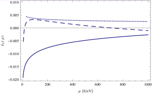
Figure 3: Corrections of orders O⁡(α)O(\alpha) (solid lines), O⁡(α​αs)O(\alpha\alpha_{s}) (long-dashed lines), and O⁡(α2)O(\alpha^{2}) (short-dashed lines) to (a) mY,b​(μ)/Mbm_{Y,b}(\mu)/M_{b} and (b) and mY,t​(μ)/Mtm_{Y,t}(\mu)/M_{t} given in Eqs. (16) and (19), respectively, as functions of μ\mu. The O⁡(α2)O(\alpha^{2}) corrections are evaluated in the gaugeless-limit approximation. The QCD corrections are not shown.

We now turn to the MS¯\overline{\rm MS} Yukawa couplings or, equivalently, the Yukawa masses mY​(μ)m_{Y}(\mu). In Figs. 3(a) and (b), we display the corrections of orders O⁡(α)O(\alpha), O⁡(α​αs)O(\alpha\alpha_{s}), and O⁡(α2)O(\alpha^{2}) to mY,b​(μ)/Mbm_{Y,b}(\mu)/M_{b} and mY,t​(μ)/Mtm_{Y,t}(\mu)/M_{t} given in Eqs. (16) and (19), respectively, as functions of μ\mu. We observe that, in the case of the bottom quark, the O⁡(α2)O(\alpha^{2}) correction exceeds the O⁡(α​αs)O(\alpha\alpha_{s}) one in size over a large μ\mu range, while, in the case of the top quark, the O⁡(α2)O(\alpha^{2}) correction is always much smaller than the O⁡(α​αs)O(\alpha\alpha_{s}) one. At the thresholds μ=Mb,Mt\mu=M_{b},M_{t}, where Eqs. (16) and (19) act as matching conditions for the RG evolution of the MS¯\overline{\rm MS} Yukawa couplings, we have77 7 In Eq. (2.49) of Ref. [33], a numerical interpolation formula for yt​(μ)y_{t}(\mu) including also the O⁡(α2)O(\alpha^{2}) correction may be found. Unfortunately, the O⁡(α)O(\alpha) and O⁡(α2)O(\alpha^{2}) corrections are not distinguished there. Since their sum is greatly dominated by the O⁡(α)O(\alpha) correction, the O⁡(α2)O(\alpha^{2}) one cannot be extracted reliably enough to allow for any meaningful comparison with our result in Eq. (19).

mY,b​(Mb)Mb\displaystyle\frac{m_{Y,b}(M_{b})}{M_{b}} =\displaystyle= 1+δQCD​(Mb)−0.0197−0.0113+0.0057,\displaystyle 1+\delta_{\rm QCD}(M_{b})-0.0197-0.0113+0.0057\,, (33)
mY,t​(Mt)Mt\displaystyle\frac{m_{Y,t}(M_{t})}{M_{t}} =\displaystyle= 1+δQCD​(Mt)+0.0013−0.0004+0.0003,\displaystyle 1+\delta_{\rm QCD}(M_{t})+0.0013-0.0004+0.0003\,, (34)

where the last three numbers on the right-hand sides represent the O⁡(α)O(\alpha), O⁡(α​αs)O(\alpha\alpha_{s}), and O⁡(α2)O(\alpha^{2}) corrections. In contrast to m⁡(μ)m(\mu), mY​(μ)m_{Y}(\mu) is devoid of leading tadpole contributions as per construction in Eq. (14). As a consequence, the electroweak corrections to mY​(μ)/Mm_{Y}(\mu)/M are considerably smaller in size than those to m⁡(μ)/Mm(\mu)/M, as is evident from the comparisons of Eq. (32) with Eq. (33) for the bottom quark and of Table 1 with Eq. (34) for the top quark. By the same token, the gaugeless-limit approximation is expected to be less reliable for mY​(μ)/Mm_{Y}(\mu)/M than for m⁡(μ)/Mm(\mu)/M, in the sense that its relative deviation from the full SM result is larger, while the absolute deviation may be similar. In the remainder of this section, we investigate this issue quantitatively, using again the one-loop results as benchmarks. From the full-SM and gaugeless-limit formulas in Ref. [10], we obtain

[mY,b​(μ)Mb−1]O⁡(α)\displaystyle\left[\frac{m_{Y,b}(\mu)}{M_{b}}-1\right]_{O(\alpha)} =\displaystyle= {−0.0490+0.0097×ln⁡(μ⁡[GeV])g.l.−0.0244+0.0031×ln⁡(μ⁡[GeV])full,\displaystyle\left\{{-0.0490+0.0097\times\ln(\mu[\mbox{GeV}])\qquad\mbox{g.l.}\atop-0.0244+0.0031\times\ln(\mu[\mbox{GeV}])\qquad\mbox{full}}\right.\,, (35)
[mY,t​(μ)Mt−1]O⁡(α)\displaystyle\left[\frac{m_{Y,t}(\mu)}{M_{t}}-1\right]_{O(\alpha)} =\displaystyle= {−0.141+0.029×ln⁡(μ⁡[GeV])g.l.−0.111+0.022×ln⁡(μ⁡[GeV])full.\displaystyle\left\{{-0.141+0.029\times\ln(\mu[\mbox{GeV}])\qquad\mbox{g.l.}\atop-0.111+0.022\times\ln(\mu[\mbox{GeV}])\qquad\mbox{full}}\right.\,. (36)

At first sight, the agreement still seems to be good, especially for the top quark. However, evaluating Eq. (35) at μ=Mb\mu=M_{b}, we obtain −0.0336-0.0336 versus −0.0195-0.0195, i.e. a relative deviation of more than 70%, and evaluating Eq. (36) at μ=Mt\mu=M_{t}, we obtain 0.0098 versus 0.0013, i.e. a relative deviation of more than 700%. Obviously, the O⁡(α2)O(\alpha^{2}) corrections displayed in Fig. 3 have to be taken with a grain of salt. While they allow us to estimate the residual theoretical uncertainties more reliably, their numerical values are only indicative. We conclude that the electroweak perturbative expansions of mY​(μ)/Mm_{Y}(\mu)/M for the bottom and top quarks exhibit useful convergence behaviors, while the O⁡(α2)O(\alpha^{2}) terms require more work.

7 Conclusion

In this paper, we calculated the electroweak corrections to the relationships between the MS¯\overline{\rm MS} masses m⁡(μ)m(\mu) and Yukawa couplings y⁡(μ)y(\mu) of the bottom and top quarks and their pole masses MM at two loops in the gaugeless limit of the SM.

We verified at one loop that the gaugeless limit provides a reliable approximation for the MS¯\overline{\rm MS} masses m⁡(μ)m(\mu). In the top-quark case, the new O⁡(α2)O(\alpha^{2}) correction induces a shift of about −0.5-0.5 GeV in mass difference mt​(Mt)−Mtm_{t}(M_{t})-M_{t} and reduces its theoretical uncertainty down to the order of 100 MeV. In the bottom-quark case, however, the new O⁡(α2)O(\alpha^{2}) correction is nearly as large in size as the O⁡(α)O(\alpha) one, indicating that the convergence property of the perturbative expansion is jeopardized by the tadpole contributions.

Detailed inspection revealed that the bulk of the corrections to the mass difference m⁡(M)−Mm(M)-M originates from the tadpole contributions, which are shared by the quantity Δ​r¯​(μ)\Delta\bar{r}(\mu) defined in Eq. (9). Owing to cancellations on the right-hand side of Eq. (14), the relationship between y⁡(μ)y(\mu) and MM is devoid of leading tadpole contributions, which motivated our proposition to measure the running of the heavy-quark masses by using y⁡(μ)y(\mu) after appropriate rescaling, as in Eq. (13). We called this new mass parameter Yukawa mass mY​(μ)m_{Y}(\mu). In fact, the electroweak corrections to the mass difference mY​(M)−Mm_{Y}(M)-M are typically one order of magnitude smaller than those to m⁡(M)−Mm(M)-M. While this considerably improves the convergence properties of the electroweak perturbation expansions, especially for the bottom quark, it greatly reduces the usefulness of the gaugeless-limit approximation, as we demonstrated at one loop. In the top-quark case, we found the O⁡(α2)O(\alpha^{2}) correction thus estimated to be small against the O⁡(α)O(\alpha) one, but comparable to the O⁡(α​αs)O(\alpha\alpha_{s}) one. In the bottom-quark case, the hierarchy among the O⁡(α)O(\alpha), O⁡(α​αs)O(\alpha\alpha_{s}), and O⁡(α2)O(\alpha^{2}) corrections turned out as naïvely expected.

Acknowledgements

The authors thank M.Yu. Kalmykov for fruitful discussions. This work was supported in part by the German Federal Ministry of Education and Research BMBF through Grant No. 05H12GUE and by the German Research Foundation DFG through the Collaborative Research Centre No. SFB 676 Particles, Strings and the Early Universe: the Structure of Matter and Space-Time.

Appendix A 𝚫​𝒓¯​(𝝁)\Delta\bar{r}(\mu) in the 𝐌𝐒¯\overline{\rm MS} scheme

In this appendix, we present the electroweak parameter 𝚫​𝒓¯\Delta\bar{r} appearing in Eq. (9) through two loops in the SM. In the following, all masses and couplings are the running quantities defined in the 𝐌𝐒¯\overline{\rm MS} scheme. To simplify the notation, the argument 𝝁\mu is always omitted. We thus need to specify the coefficients 𝒙𝟏,𝟎x_{1,0}, 𝒙𝟏,𝟏x_{1,1}, and 𝒙𝟐,𝟎x_{2,0} in the perturbative expansion

𝚫​𝒓¯=𝒈𝟐𝟏𝟔​𝝅𝟐​𝒙𝟏,𝟎+𝑪𝑭​𝒈𝒔𝟐𝟏𝟔​𝝅𝟐​𝒈𝟐𝟏𝟔​𝝅𝟐​𝒙𝟏,𝟏+(𝒈𝟐𝟏𝟔​𝝅𝟐)𝟐​𝒙𝟐,𝟎+⋯,\Delta\bar{r}=\frac{g^{2}}{16\pi^{2}}\,x_{1,0}+C_{F}\frac{g_{s}^{2}}{16\pi^{2}}\frac{g^{2}}{16\pi^{2}}\,x_{1,1}+\left(\frac{g^{2}}{16\pi^{2}}\right)^{2}x_{2,0}+\cdots\,, (37)

where 𝒈=𝒆¯/𝒔𝒘g=\bar{e}/s_{w} and 𝒈𝒔g_{s} are the electroweak and strong-coupling constants in the 𝐌𝐒¯\overline{\rm MS} scheme.

The coefficients 𝒙𝟏,𝟎x_{1,0} and 𝒙𝟏,𝟏x_{1,1} may be given in exact form:

𝒙𝟏,𝟎\displaystyle x_{1,0} =\displaystyle= 𝑵𝒄​𝟐​𝒎𝒕𝟒𝒎𝑾𝟐​𝒎𝑯𝟐​(𝟏−𝒍𝒕)−𝑵𝒄​𝒎𝒕𝟐𝒎𝑾𝟐​(𝟏𝟒−𝟏𝟐​𝒍𝒕)+𝟑𝟒​𝒎𝑾𝟐𝒎𝑯𝟐−𝒎𝑾𝟐​𝐥𝐧⁡𝒎𝑾𝟐𝒎𝑯𝟐\displaystyle N_{c}\frac{2m_{t}^{4}}{m_{W}^{2}m_{H}^{2}}(1-l_{t})-N_{c}\frac{m_{t}^{2}}{m_{W}^{2}}\Big(\frac{1}{4}-\frac{1}{2}l_{t}\Big)+\frac{3}{4}\frac{m_{W}^{2}}{m_{H}^{2}-m_{W}^{2}}\ln\frac{m_{W}^{2}}{m_{H}^{2}}
+𝒎𝑯𝟐𝒎𝑾𝟐​(−𝟕𝟖+𝟑𝟒​𝒍𝒉)+𝒎𝑾𝟐𝒎𝑯𝟐​(−𝟏−𝟏𝟐​𝒄𝒘𝟒+𝟑​𝒍𝒘+𝟑𝟐​𝒄𝒘𝟒​𝒍𝒛)\displaystyle+\frac{m_{H}^{2}}{m_{W}^{2}}\Big(-\frac{7}{8}+\frac{3}{4}l_{h}\Big)+\frac{m_{W}^{2}}{m_{H}^{2}}\Big(-1-\frac{1}{2c_{w}^{4}}+3l_{w}+\frac{3}{2c_{w}^{4}}l_{z}\Big)
+𝟓𝟒+𝟓𝟖​𝒄𝒘𝟐−𝟑𝟒​𝒔𝒘𝟐​𝐥𝐧⁡𝒄𝒘𝟐−𝟑𝟒​𝒍𝒉−𝟑𝟒​𝒍𝒘−𝟑𝟒​𝒄𝒘𝟐​𝒍𝒛,\displaystyle+\frac{5}{4}+\frac{5}{8c_{w}^{2}}-\frac{3}{4s_{w}^{2}}\ln c_{w}^{2}-\frac{3}{4}l_{h}-\frac{3}{4}l_{w}-\frac{3}{4c_{w}^{2}}l_{z}\,,
𝒙𝟏,𝟏\displaystyle x_{1,1} =\displaystyle= 𝑵𝒄​𝒎𝒕𝟒𝒎𝑾𝟐​𝒎𝑯𝟐​(𝟐𝟎−𝟐𝟎​𝒍𝒕+𝟏𝟐​𝒍𝒕𝟐)+𝑵𝒄​𝒎𝒕𝟐𝒎𝑾𝟐​(−𝟏𝟑𝟖+𝜻𝟐+𝒍𝒕−𝟑𝟐​𝒍𝒕𝟐),\displaystyle N_{c}\frac{m_{t}^{4}}{m_{W}^{2}m_{H}^{2}}(20-20l_{t}+12l_{t}^{2})+N_{c}\frac{m_{t}^{2}}{m_{W}^{2}}\Big(-\frac{13}{8}+\zeta_{2}+l_{t}-\frac{3}{2}l_{t}^{2}\Big)\,, (38)

where, in analogy with the definitions introduced below Eq. (16), 𝒍𝒙=𝐥𝐧⁡(𝒎𝒙𝟐/𝝁𝟐)l_{x}=\ln(m_{x}^{2}/\mu^{2}), 𝒄𝒘=𝒎𝑾/𝒎𝒁c_{w}=m_{W}/m_{Z}, and 𝒔𝒘=𝟏−𝒄𝒘𝟐s_{w}=\sqrt{1-c_{w}^{2}}.

The two-loop electroweak correction 𝒙𝟐,𝟎x_{2,0} in the full SM with arbitrary particle masses may be expressed in terms of dilogarithms. However the result is too lengthy to be presented here. Instead, we evaluate 𝒙𝟐,𝟎x_{2,0} in two different approximations: the gaugeless limit of the SM, 𝒙𝟐,𝟎𝐠𝐥x_{2,0}^{\rm gl}, and the heavy-top-quark limit, 𝒙𝟐,𝟎𝐡𝐭x_{2,0}^{\rm ht}. In the former case, we have

𝒙𝟐,𝟎𝐠𝐥\displaystyle x_{2,0}^{\rm gl} =\displaystyle= 𝟒​𝑵𝒄𝟐​𝒎𝒕𝟖𝒎𝑯𝟒​𝒎𝑾𝟒(𝟏−𝒍𝒕)+𝑵𝒄​𝒎𝒕𝟔𝒎𝑯𝟐​𝒎𝑾𝟒{𝑵𝒄𝟐(𝟏−𝒍𝒕)(−𝟑+𝟐𝒍𝒕)−𝟒𝟓𝟑𝟐𝒍𝒕𝟐+𝟑𝟑𝟐𝒍𝒉𝟐\displaystyle\frac{4N_{c}^{2}m_{t}^{8}}{m_{H}^{4}m_{W}^{4}}(1-l_{t})+\frac{N_{c}m_{t}^{6}}{m_{H}^{2}m_{W}^{4}}\Bigg\{\frac{N_{c}}{2}(1-l_{t})(-3+2l_{t})-\frac{45}{32}l_{t}^{2}+\frac{3}{32}l_{h}^{2} (39)
−𝟑𝟏𝟔𝒍𝒕𝒍𝒉+𝟏𝟑𝟐𝒍𝒕−𝟓𝟖𝜻𝟐−𝟏𝟓𝟐−𝟑𝟏𝟔ℋ(𝒉𝒕)+𝟗𝟐𝚽(𝒉𝒕/𝟒)}\displaystyle-\frac{3}{16}l_{t}l_{h}+\frac{13}{2}l_{t}-\frac{5}{8}\zeta_{2}-\frac{15}{2}-\frac{3}{16}{\cal H}(h_{t})+\frac{9}{2}\Phi(h_{t}/4)\Bigg\}
+𝑵𝒄𝒎𝒕𝟒𝒎𝑾𝟒{(𝟏𝟒𝟏𝟔𝟒−𝟑𝟏𝟔𝒉𝒕−𝟑𝟔𝟒𝒉𝒕𝟐+𝑵𝒄𝟒)𝒍𝒕𝟐+(−𝟏𝟓𝟔𝟒+𝟑𝟏𝟔𝒉𝒕−𝟑𝟔𝟒𝒉𝒕𝟐)𝒍𝒉𝟐\displaystyle+N_{c}\frac{m_{t}^{4}}{m_{W}^{4}}\Bigg\{\Big(\frac{141}{64}-\frac{3}{16}h_{t}-\frac{3}{64}h_{t}^{2}+\frac{N_{c}}{4}\Big)l_{t}^{2}+\Big(-\frac{15}{64}+\frac{3}{16}h_{t}-\frac{3}{64}h_{t}^{2}\Big)l_{h}^{2}
+(−𝟖𝟏𝟑𝟐+𝟑𝟒​𝒉𝒕+𝟑𝟑𝟐​𝒉𝒕𝟐)​𝒍𝒕​𝒍𝒉+(−𝟓𝟒−𝟏𝟏𝟏𝟔​𝒉𝒕−𝑵𝒄𝟒)​𝒍𝒕\displaystyle+\Big(-\frac{81}{32}+\frac{3}{4}h_{t}+\frac{3}{32}h_{t}^{2}\Big)l_{t}l_{h}+\Big(-\frac{5}{4}-\frac{11}{16}h_{t}-\frac{N_{c}}{4}\Big)l_{t}
+(𝟒𝟑𝟖−𝟐𝟓𝟏𝟔​𝒉𝒕)​𝒍𝒉+𝑵𝒄𝟏𝟔+𝟕𝟏𝟔​𝜻𝟐−𝟐𝟗𝟓𝟔𝟒+𝟏𝟕𝟖​𝒉𝒕\displaystyle+\Big(\frac{43}{8}-\frac{25}{16}h_{t}\Big)l_{h}+\frac{N_{c}}{16}+\frac{7}{16}\zeta_{2}-\frac{295}{64}+\frac{17}{8}h_{t}
+(𝟏𝟓𝟑𝟐−𝟑𝟖𝒉𝒕+𝟑𝟑𝟐𝒉𝒕𝟐)ℋ(𝒉𝒕)+(−𝟏𝟓𝟖−𝟑𝟏𝟔𝒉𝒕+𝟑𝟑𝟐𝒉𝒕𝟐)𝚽(𝒉𝒕/𝟒)}\displaystyle+\Big(\frac{15}{32}-\frac{3}{8}h_{t}+\frac{3}{32}h_{t}^{2}\Big){\cal H}(h_{t})+\Big(-\frac{15}{8}-\frac{3}{16}h_{t}+\frac{3}{32}h_{t}^{2}\Big)\Phi(h_{t}/4)\Bigg\}
+𝒎𝑯𝟒𝒎𝑾𝟒​{𝟐𝟕𝟑𝟐​𝒍𝒉𝟐−𝟐𝟕𝟖​𝒍𝒉+𝟏𝟒​𝜻𝟐−𝟐𝟒𝟑𝟑𝟐​𝑺𝟐+𝟒𝟓𝟕𝟏𝟐𝟖},\displaystyle+\frac{m_{H}^{4}}{m_{W}^{4}}\Bigg\{\frac{27}{32}l_{h}^{2}-\frac{27}{8}l_{h}+\frac{1}{4}\zeta_{2}-\frac{243}{32}S_{2}+\frac{457}{128}\Bigg\}\,,

where 𝒉𝒕=𝒎𝑯𝟐/𝒎𝒕𝟐h_{t}=m_{H}^{2}/m_{t}^{2}. In the latter case, we obtain

𝒙𝟐,𝟎𝐡𝐭\displaystyle x_{2,0}^{\rm ht} =\displaystyle= 𝑵𝒄{𝑵𝒄𝟒​𝒎𝒕𝟖𝒎𝑾𝟒​𝒎𝑯𝟐(𝟏−𝒍𝒕)+𝒎𝒕𝟔𝒎𝑾𝟒​𝒎𝑯𝟐(−𝟏𝟓𝟐−𝜻𝟐+𝟏𝟑𝟐𝒍𝒕−𝟑𝟐𝒍𝒕𝟐\displaystyle N_{c}\Bigg\{N_{c}\frac{4m_{t}^{8}}{m_{W}^{4}m_{H}^{2}}(1-l_{t})+\frac{m_{t}^{6}}{m_{W}^{4}m_{H}^{2}}\Bigg(-\frac{15}{2}-\zeta_{2}+\frac{13}{2}l_{t}-\frac{3}{2}l_{t}^{2} (40)
OPEN+𝑵𝒄𝟐​(𝟏−𝒍𝒕)​(−𝟑+𝟐​𝒍𝒕))+𝒎𝒕𝟒(𝒎𝑯𝟐−𝒎𝑾𝟐)𝟐​(𝟑𝟒​𝒍𝒉𝟐−𝟑𝟒​𝒍𝒘𝟐+𝟑​𝒍𝒘​𝒉​𝒍𝒕)\displaystyle+\frac{N_{c}}{2}(1-l_{t})(-3+2l_{t})\Bigg)+\frac{m_{t}^{4}}{(m_{H}^{2}-m_{W}^{2})^{2}}\Big(\frac{3}{4}l_{h}^{2}-\frac{3}{4}l_{w}^{2}+3l_{wh}l_{t}\Big)
+𝒎𝒕𝟒𝒎𝑾𝟐​(𝒎𝑯𝟐−𝒎𝑾𝟐)​(𝟑𝟐​𝒍𝒘​(𝟏−𝒍𝒕)+𝟑𝟐​(𝒍𝒕−𝒍𝒉)+𝟑𝟖​(𝒍𝒕+𝒍𝒉)𝟐)\displaystyle+\frac{m_{t}^{4}}{m_{W}^{2}(m_{H}^{2}-m_{W}^{2})}\Big(\frac{3}{2}l_{w}(1-l_{t})+\frac{3}{2}(l_{t}-l_{h})+\frac{3}{8}(l_{t}+l_{h})^{2}\Bigg)
+𝒎𝒕𝟒𝒎𝑯𝟒​(−𝟖−𝟒𝒄𝒘𝟒+𝟔​𝒍𝒘+𝟔​𝒍𝒕+𝟑𝒄𝒘𝟒​(𝒍𝒕+𝒍𝒛))\displaystyle+\frac{m_{t}^{4}}{m_{H}^{4}}\Big(-8-\frac{4}{c_{w}^{4}}+6l_{w}+6l_{t}+\frac{3}{c_{w}^{4}}(l_{t}+l_{z})\Big)
+𝒎𝒕𝟒𝒎𝑾𝟐​𝒎𝑯𝟐​(𝟒𝟑​𝒔𝒘𝟐𝒄𝒘𝟐​𝒍𝒕𝟐+(𝟏−𝒍𝒕)​(𝟓𝟗𝟏𝟖+𝟏𝟕𝟗𝟑𝟔​𝒄𝒘𝟐−𝟑𝟐​𝒔𝑾𝟐​𝐥𝐧⁡𝒄𝒘𝟐−𝟑𝟐​𝒄𝒘𝟐​𝒍𝒛−𝟑​𝒍𝒘))\displaystyle+\frac{m_{t}^{4}}{m_{W}^{2}m_{H}^{2}}\Bigg(\frac{4}{3}\frac{s_{w}^{2}}{c_{w}^{2}}l_{t}^{2}+(1-l_{t})\Big(\frac{59}{18}+\frac{179}{36c_{w}^{2}}-\frac{3}{2s_{W}^{2}}\ln c_{w}^{2}-\frac{3}{2c_{w}^{2}}l_{z}-3l_{w}\Big)\Bigg)
+𝒎𝒕𝟒𝒎𝑾𝟒​(𝑵𝒄​(𝟏𝟏𝟔−𝟏𝟒​𝒍𝒕​(𝟏−𝒍𝒕))+𝟑𝟎𝟓𝟔𝟒+𝟏𝟏𝟖​𝜻𝟐+𝟏𝟐​𝒍𝒉+𝟗𝟖​𝒍𝒉𝟐CLOSE\displaystyle+\frac{m_{t}^{4}}{m_{W}^{4}}\Bigg(N_{c}\Big(\frac{1}{16}-\frac{1}{4}l_{t}(1-l_{t})\Big)+\frac{305}{64}+\frac{11}{8}\zeta_{2}+\frac{1}{2}l_{h}+\frac{9}{8}l_{h}^{2}
−𝟐𝟏𝟒𝒍𝒉𝒍𝒕+𝟐𝟗𝟖𝒍𝒕+𝟓𝟕𝟏𝟔𝒍𝒕𝟐)}+𝑶(𝒎𝒕𝟐).\displaystyle-\frac{21}{4}l_{h}l_{t}+\frac{29}{8}l_{t}+\frac{57}{16}l_{t}^{2}\Bigg)\Bigg\}+O(m_{t}^{2})\,.

In Eq. (39), two new functions have been introduced. They correspond to two-loop vacuum bubble integrals with two different masses, namely 𝑱⁡(𝟎,𝒎𝟏𝟐,𝒎𝟐𝟐)J(0,m_{1}^{2},m_{2}^{2}) and 𝑱⁡(𝒎𝟏𝟐,𝒎𝟐𝟐,𝒎𝟐𝟐)J(m_{1}^{2},m_{2}^{2},m_{2}^{2}). Adopting the notations from Ref. [34] with 𝒛=𝒎𝟏𝟐/𝒎𝟐𝟐z=m_{1}^{2}/m_{2}^{2} and from Ref. [35] with 𝒛=𝒎𝟏𝟐/(𝟒​𝒎𝟐𝟐)z=m_{1}^{2}/(4m_{2}^{2}), they are given by

ℋ⁡(𝒛)\displaystyle{\cal H}(z) =\displaystyle= 𝟐​𝐋​𝐢𝟐​(𝟏−𝒛)+𝟏𝟐​𝐥𝐧𝟐​𝒛,\displaystyle 2{\rm Li}_{2}(1-z)+\frac{1}{2}\ln^{2}z\,, (41)
𝚽⁡(𝒛)\displaystyle\Phi(z) =\displaystyle= 𝟒​𝒛𝟏−𝒛​𝐂𝐥𝟐​(𝟐​𝐚𝐫𝐜𝐬𝐢𝐧⁡𝒛),\displaystyle 4\sqrt{\frac{z}{1-z}}{\rm Cl}_{2}(2\arcsin\sqrt{z}), (42)

respectively, where

𝐂𝐥𝟐(𝜽)=−∫𝟎𝜽𝒅𝜽′𝐥𝐧(𝟐𝐬𝐢𝐧𝜽′𝟐){\rm Cl}_{2}(\theta)=-\int\limits_{0}^{\theta}d\theta^{\prime}\ln\left(2\sin\frac{\theta^{\prime}}{2}\right) (43)

is Clausen’s integral [36].

Appendix B Renormalization constants of the quark masses

The calculations presented in this paper require the renormalizations of the bottom- and top-quark masses through two loops and of all other masses and couplings at one loop. For our purposes, knowledge of the corresponding renormalization constants in the approximations of the gaugeless and heavy-top-quark limits is sufficient. However, we also calculated the mass renormalization constants 𝒁𝒎Z_{m} of the bottom and top quarks exactly at two loops in the SM. For future applications and checks, we present our results in the following. In the 𝐌𝐒¯\overline{\rm MS} scheme, 𝒁𝒎Z_{m} is defined as

𝒁𝒎=[𝒎𝟎𝒎⁡(𝝁)]𝟐,Z_{m}=\left[\frac{m^{0}}{m(\mu)}\right]^{2}, (44)

and may be written in the form

𝒁𝒎\displaystyle Z_{m} =\displaystyle= 𝟏+𝒈𝟐𝟏𝟔​𝝅𝟐​𝒁𝜶(𝟏,𝟏)𝜺+𝑪𝑭​𝒈𝒔𝟐𝟏𝟔​𝝅𝟐​𝒁𝜶𝒔(𝟏,𝟏)𝜺\displaystyle 1+\frac{g^{2}}{16\pi^{2}}\frac{Z_{\alpha}^{(1,1)}}{\varepsilon}+C_{F}\frac{g_{s}^{2}}{16\pi^{2}}\frac{Z_{\alpha_{s}}^{(1,1)}}{\varepsilon} (45)
+𝑪𝑭​𝒈𝟐𝟏𝟔​𝝅𝟐​𝒈𝒔𝟐𝟏𝟔​𝝅𝟐​(𝒁𝜶​𝜶𝒔(𝟐,𝟐)𝜺𝟐+𝒁𝜶​𝜶𝒔(𝟐,𝟏)𝜺)+(𝒈𝟐𝟏𝟔​𝝅𝟐)𝟐​(𝒁𝜶𝟐(𝟐,𝟐)𝜺𝟐+𝒁𝜶𝟐(𝟐,𝟏)𝜺)+⋯.\displaystyle+C_{F}\frac{g^{2}}{16\pi^{2}}\frac{g_{s}^{2}}{16\pi^{2}}\left(\frac{Z_{\alpha\alpha_{s}}^{(2,2)}}{\varepsilon^{2}}+\frac{Z_{\alpha\alpha_{s}}^{(2,1)}}{\varepsilon}\right)+\left(\frac{g^{2}}{16\pi^{2}}\right)^{2}\left(\frac{Z_{\alpha^{2}}^{(2,2)}}{\varepsilon^{2}}+\frac{Z_{\alpha^{2}}^{(2,1)}}{\varepsilon}\right)+\cdots\,.

Using the same notation as in Appendix A, we have

𝒁𝜶(𝟏,𝟏)\displaystyle Z^{(1,1)}_{\alpha} =\displaystyle= −𝟏𝟑−𝟑𝟒​𝒎𝑯𝟐𝒎𝑾𝟐−𝟑𝟒​𝒎𝒕𝟐𝒎𝑾𝟐−𝟑​𝒎𝑾𝟐𝒎𝑯𝟐+𝟏𝟑​𝒎𝒁𝟐𝒎𝑾𝟐−𝟑𝟐​𝒎𝒁𝟒𝒎𝑯𝟐​𝒎𝑾𝟐+𝟐​𝑵𝒄​𝒎𝒕𝟒𝒎𝑯𝟐​𝒎𝑾𝟐,\displaystyle-\frac{1}{3}-\frac{3}{4}\frac{m_{H}^{2}}{m_{W}^{2}}-\frac{3}{4}\frac{m_{t}^{2}}{m_{W}^{2}}-3\frac{m_{W}^{2}}{m_{H}^{2}}+\frac{1}{3}\frac{m_{Z}^{2}}{m_{W}^{2}}-\frac{3}{2}\frac{m_{Z}^{4}}{m_{H}^{2}m_{W}^{2}}+2N_{c}\frac{m_{t}^{4}}{m_{H}^{2}m_{W}^{2}}\,, (46)
𝒁𝜶𝒔(𝟏,𝟏)\displaystyle Z^{(1,1)}_{\alpha_{s}} =\displaystyle= −𝟑,\displaystyle-3\,, (47)
𝒁𝜶​𝜶𝒔(𝟐,𝟐)\displaystyle Z^{(2,2)}_{\alpha\alpha_{s}} =\displaystyle= 𝟐+𝟗𝟐​𝒎𝑯𝟐𝒎𝑾𝟐+𝟐𝟕𝟒​𝒎𝒕𝟐𝒎𝑾𝟐+𝟏𝟖​𝒎𝑾𝟐𝒎𝑯𝟐−𝟐​𝒎𝒁𝟐𝒎𝑾𝟐+𝟗​𝒎𝒁𝟒𝒎𝑯𝟐​𝒎𝑾𝟐−𝟐𝟒​𝑵𝒄​𝒎𝒕𝟒𝒎𝑯𝟐​𝒎𝑾𝟐,\displaystyle 2+\frac{9}{2}\frac{m_{H}^{2}}{m_{W}^{2}}+\frac{27}{4}\frac{m_{t}^{2}}{m_{W}^{2}}+18\frac{m_{W}^{2}}{m_{H}^{2}}-2\frac{m_{Z}^{2}}{m_{W}^{2}}+9\frac{m_{Z}^{4}}{m_{H}^{2}m_{W}^{2}}-24N_{c}\frac{m_{t}^{4}}{m_{H}^{2}m_{W}^{2}}\,, (48)
𝒁𝜶​𝜶𝒔(𝟐,𝟏)\displaystyle Z^{(2,1)}_{\alpha\alpha_{s}} =\displaystyle= 𝟐𝟓𝟏𝟐−𝟑​𝒎𝒕𝟐𝒎𝑾𝟐+𝟑𝟏𝟐𝟒​𝒎𝒁𝟐𝒎𝑾𝟐+𝟒​𝑵𝒄​𝒎𝒕𝟒𝒎𝑯𝟐​𝒎𝑾𝟐,\displaystyle\frac{25}{12}-3\frac{m_{t}^{2}}{m_{W}^{2}}+\frac{31}{24}\frac{m_{Z}^{2}}{m_{W}^{2}}+4N_{c}\frac{m_{t}^{4}}{m_{H}^{2}m_{W}^{2}}\,, (49)
𝒁𝜶𝟐(𝟐,𝟐)\displaystyle Z^{(2,2)}_{\alpha^{2}} =\displaystyle= 𝟖𝟑𝟐𝟒+𝟗𝟏𝟔​𝒎𝑯𝟐​𝒎𝒕𝟐𝒎𝑾𝟒−𝟗𝟑𝟐​𝒎𝑯𝟒𝒎𝑾𝟒+𝟗𝟑𝟐​𝒎𝒁𝟐​𝒎𝒕𝟐𝒎𝑾𝟒+𝟓𝟏𝟔​𝒎𝒁𝟐​𝒎𝑯𝟐𝒎𝑾𝟒+𝟗𝟖​𝒎𝒁𝟒𝒎𝑾𝟒​𝒎𝒕𝟐𝒎𝑯𝟐\displaystyle\frac{83}{24}+\frac{9}{16}\frac{m_{H}^{2}m_{t}^{2}}{m_{W}^{4}}-\frac{9}{32}\frac{m_{H}^{4}}{m_{W}^{4}}+\frac{9}{32}\frac{m_{Z}^{2}m_{t}^{2}}{m_{W}^{4}}+\frac{5}{16}\frac{m_{Z}^{2}m_{H}^{2}}{m_{W}^{4}}+\frac{9}{8}\frac{m_{Z}^{4}}{m_{W}^{4}}\frac{m_{t}^{2}}{m_{H}^{2}} (50)
+𝟖𝟓𝟒𝟖​𝒎𝒁𝟒𝒎𝑾𝟒−𝟏𝟓𝟖​𝒎𝒁𝟔𝒎𝑾𝟒​𝒎𝑯𝟐+𝟗𝟒​𝒎𝒁𝟖𝒎𝑾𝟒​𝒎𝑯𝟒+𝟗𝟏𝟔​𝒎𝒕𝟐𝒎𝑾𝟐+𝟏𝟏𝟖​𝒎𝑯𝟐𝒎𝑾𝟐−𝟏𝟔​𝒎𝒁𝟐𝒎𝑾𝟐\displaystyle{}+\frac{85}{48}\frac{m_{Z}^{4}}{m_{W}^{4}}-\frac{15}{8}\frac{m_{Z}^{6}}{m_{W}^{4}m_{H}^{2}}+\frac{9}{4}\frac{m_{Z}^{8}}{m_{W}^{4}m_{H}^{4}}+\frac{9}{16}\frac{m_{t}^{2}}{m_{W}^{2}}+\frac{11}{8}\frac{m_{H}^{2}}{m_{W}^{2}}-\frac{1}{6}\frac{m_{Z}^{2}}{m_{W}^{2}}
−𝟓𝟒​𝒎𝒁𝟒𝒎𝑾𝟐​𝒎𝑯𝟐+𝟗𝟒​𝒎𝒕𝟐𝒎𝑯𝟐+𝟐𝟗𝟒​𝒎𝒁𝟐𝒎𝑯𝟐+𝟗​𝒎𝒁𝟒𝒎𝑯𝟒+𝟏𝟖​𝒎𝑾𝟐𝒎𝑯𝟐+𝟗​𝒎𝑾𝟒𝒎𝑯𝟒\displaystyle{}-\frac{5}{4}\frac{m_{Z}^{4}}{m_{W}^{2}m_{H}^{2}}+\frac{9}{4}\frac{m_{t}^{2}}{m_{H}^{2}}+\frac{29}{4}\frac{m_{Z}^{2}}{m_{H}^{2}}+9\frac{m_{Z}^{4}}{m_{H}^{4}}+18\frac{m_{W}^{2}}{m_{H}^{2}}+9\frac{m_{W}^{4}}{m_{H}^{4}}
+𝒏𝑮​(𝟏𝟔+𝟏𝟔​𝒎𝒁𝟒𝒎𝑾𝟒−𝟑𝟐​𝒎𝒁𝟔𝒎𝑾𝟒​𝒎𝑯𝟐−𝟏𝟑​𝒎𝒁𝟐𝒎𝑾𝟐+𝟑​𝒎𝒁𝟒𝒎𝑾𝟐​𝒎𝑯𝟐−𝟐​𝒎𝒁𝟐𝒎𝑯𝟐−𝒎𝑾𝟐𝒎𝑯𝟐)\displaystyle{}+n_{G}\Bigg(\frac{1}{6}+\frac{1}{6}\frac{m_{Z}^{4}}{m_{W}^{4}}-\frac{3}{2}\frac{m_{Z}^{6}}{m_{W}^{4}m_{H}^{2}}-\frac{1}{3}\frac{m_{Z}^{2}}{m_{W}^{2}}+3\frac{m_{Z}^{4}}{m_{W}^{2}m_{H}^{2}}-2\frac{m_{Z}^{2}}{m_{H}^{2}}-\frac{m_{W}^{2}}{m_{H}^{2}}\Bigg)
+𝑵𝒄​(−𝟑𝟗𝟏𝟔​𝒎𝒕𝟒𝒎𝑾𝟒−𝟑𝟖​𝒎𝑯𝟐​𝒎𝒕𝟐𝒎𝑾𝟒−𝟐𝟑​𝒎𝒁𝟐​𝒎𝒕𝟒𝒎𝑾𝟒​𝒎𝑯𝟐−𝟔​𝒎𝒁𝟒​𝒎𝒕𝟒𝒎𝑾𝟒​𝒎𝑯𝟒+𝟑𝟒​𝒎𝒁𝟒​𝒎𝒕𝟐𝒎𝑾𝟒​𝒎𝑯𝟐CLOSE\displaystyle{}+N_{c}\Bigg(-\frac{39}{16}\frac{m_{t}^{4}}{m_{W}^{4}}-\frac{3}{8}\frac{m_{H}^{2}m_{t}^{2}}{m_{W}^{4}}-\frac{2}{3}\frac{m_{Z}^{2}m_{t}^{4}}{m_{W}^{4}m_{H}^{2}}-6\frac{m_{Z}^{4}m_{t}^{4}}{m_{W}^{4}m_{H}^{4}}+\frac{3}{4}\frac{m_{Z}^{4}m_{t}^{2}}{m_{W}^{4}m_{H}^{2}}
OPEN+𝟐𝟑​𝒎𝒕𝟒𝒎𝑾𝟐​𝒎𝑯𝟐−𝟏𝟐​𝒎𝒕𝟒𝒎𝑯𝟒+𝟑𝟐​𝒎𝒕𝟐𝒎𝑯𝟐)+𝑵𝒄​𝒏𝑮​(𝟏𝟏𝟏𝟔𝟐+𝟏𝟏𝟏𝟔𝟐​𝒎𝒁𝟒𝒎𝑾𝟒−𝟏𝟏𝟏𝟖​𝒎𝒁𝟔𝒎𝑾𝟒​𝒎𝑯𝟐CLOSE\displaystyle{}+\frac{2}{3}\frac{m_{t}^{4}}{m_{W}^{2}m_{H}^{2}}-12\frac{m_{t}^{4}}{m_{H}^{4}}+\frac{3}{2}\frac{m_{t}^{2}}{m_{H}^{2}}\Bigg)+N_{c}n_{G}\Bigg(\frac{11}{162}+\frac{11}{162}\frac{m_{Z}^{4}}{m_{W}^{4}}-\frac{11}{18}\frac{m_{Z}^{6}}{m_{W}^{4}m_{H}^{2}}
OPEN−𝟏𝟏𝟖𝟏​𝒎𝒁𝟐𝒎𝑾𝟐+𝟏𝟏𝟗​𝒎𝒁𝟒𝒎𝑾𝟐​𝒎𝑯𝟐−𝟏𝟎𝟗​𝒎𝒁𝟐𝒎𝑯𝟐−𝒎𝑾𝟐𝒎𝑯𝟐)+𝟒​𝑵𝒄𝟐​𝒎𝒕𝟖𝒎𝑾𝟒​𝒎𝑯𝟒,\displaystyle{}-\frac{11}{81}\frac{m_{Z}^{2}}{m_{W}^{2}}+\frac{11}{9}\frac{m_{Z}^{4}}{m_{W}^{2}m_{H}^{2}}-\frac{10}{9}\frac{m_{Z}^{2}}{m_{H}^{2}}-\frac{m_{W}^{2}}{m_{H}^{2}}\Bigg)+4N_{c}^{2}\frac{m_{t}^{8}}{m_{W}^{4}m_{H}^{4}}\,,
𝒁𝜶𝟐(𝟐,𝟏)\displaystyle Z^{(2,1)}_{\alpha^{2}} =\displaystyle= 𝟏𝟎𝟑𝟏𝟒𝟒+𝟏𝟏𝟑𝟐​𝒎𝒕𝟒𝒎𝑾𝟒+𝟑𝟑𝟑𝟐​𝒎𝑯𝟒𝒎𝑾𝟒−𝟕𝟗𝟏𝟗𝟐​𝒎𝒁𝟐​𝒎𝒕𝟐𝒎𝑾𝟒−𝟑𝟖​𝒎𝒁𝟐​𝒎𝑯𝟐𝒎𝑾𝟒−𝟏𝟎𝟏𝟗𝟓𝟕𝟔​𝒎𝒁𝟒𝒎𝑾𝟒+𝟓𝟗𝟐𝟒​𝒎𝒁𝟔𝒎𝑾𝟒​𝒎𝒕𝟐\displaystyle\frac{103}{144}+\frac{11}{32}\frac{m_{t}^{4}}{m_{W}^{4}}+\frac{33}{32}\frac{m_{H}^{4}}{m_{W}^{4}}-\frac{79}{192}\frac{m_{Z}^{2}m_{t}^{2}}{m_{W}^{4}}-\frac{3}{8}\frac{m_{Z}^{2}m_{H}^{2}}{m_{W}^{4}}-\frac{1019}{576}\frac{m_{Z}^{4}}{m_{W}^{4}}+\frac{59}{24}\frac{m_{Z}^{6}}{m_{W}^{4}m_{t}^{2}} (51)
+𝟓𝟑𝟗𝟔​𝒎𝒕𝟐𝒎𝑾𝟐−𝟑𝟒​𝒎𝑯𝟐𝒎𝑾𝟐+𝟒𝟗​𝒎𝒁𝟐𝒎𝑾𝟐+𝟑𝟏𝟏𝟐​𝒎𝒁𝟒𝒎𝑾𝟐​𝒎𝑯𝟐−𝟏𝟕𝟐​𝒎𝒁𝟐𝒎𝑯𝟐−𝟏𝟕𝟔𝟑​𝒎𝑾𝟐𝒎𝑯𝟐\displaystyle{}+\frac{53}{96}\frac{m_{t}^{2}}{m_{W}^{2}}-\frac{3}{4}\frac{m_{H}^{2}}{m_{W}^{2}}+\frac{4}{9}\frac{m_{Z}^{2}}{m_{W}^{2}}+\frac{31}{12}\frac{m_{Z}^{4}}{m_{W}^{2}m_{H}^{2}}-\frac{17}{2}\frac{m_{Z}^{2}}{m_{H}^{2}}-\frac{176}{3}\frac{m_{W}^{2}}{m_{H}^{2}}
+𝒏𝑮​(−𝟑𝟕𝟕𝟐−𝟒𝟕𝟏𝟒𝟒​𝒎𝒁𝟒𝒎𝑾𝟒+𝟐​𝒎𝒁𝟔𝒎𝑾𝟒​𝒎𝑯𝟐+𝟒𝟕𝟕𝟐​𝒎𝒁𝟐𝒎𝑾𝟐−𝟒​𝒎𝒁𝟒𝒎𝑾𝟐​𝒎𝑯𝟐+𝟖𝟑​𝒎𝒁𝟐𝒎𝑯𝟐+𝟒𝟑​𝒎𝑾𝟐𝒎𝑯𝟐)\displaystyle{}+n_{G}\Bigg(-\frac{37}{72}-\frac{47}{144}\frac{m_{Z}^{4}}{m_{W}^{4}}+2\frac{m_{Z}^{6}}{m_{W}^{4}m_{H}^{2}}+\frac{47}{72}\frac{m_{Z}^{2}}{m_{W}^{2}}-4\frac{m_{Z}^{4}}{m_{W}^{2}m_{H}^{2}}+\frac{8}{3}\frac{m_{Z}^{2}}{m_{H}^{2}}+\frac{4}{3}\frac{m_{W}^{2}}{m_{H}^{2}}\Bigg)
+𝑵𝒄​(−𝟓𝟐​𝒎𝒕𝟔𝒎𝑾𝟒​𝒎𝑯𝟐−𝟏𝟏𝟑𝟐​𝒎𝒕𝟒𝒎𝑾𝟒+𝟑𝟖​𝒎𝑯𝟐​𝒎𝒕𝟐𝒎𝑾𝟒+𝟒𝟗​𝒎𝒁𝟐​𝒎𝒕𝟒𝒎𝑾𝟒​𝒎𝑯𝟐+𝟏𝟗𝟏𝟐​𝒎𝒁𝟒𝒎𝑾𝟒​𝒎𝒕𝟐𝒎𝑯𝟐CLOSE\displaystyle{}+N_{c}\Bigg(-\frac{5}{2}\frac{m_{t}^{6}}{m_{W}^{4}m_{H}^{2}}-\frac{11}{32}\frac{m_{t}^{4}}{m_{W}^{4}}+\frac{3}{8}\frac{m_{H}^{2}m_{t}^{2}}{m_{W}^{4}}+\frac{4}{9}\frac{m_{Z}^{2}m_{t}^{4}}{m_{W}^{4}m_{H}^{2}}+\frac{19}{12}\frac{m_{Z}^{4}}{m_{W}^{4}}\frac{m_{t}^{2}}{m_{H}^{2}}
OPEN−𝟒𝟗​𝒎𝒕𝟒𝒎𝑾𝟐​𝒎𝑯𝟐−𝟐𝟎𝟑​𝒎𝒁𝟐​𝒎𝒕𝟐𝒎𝑾𝟐​𝒎𝑯𝟐+𝟑𝟓𝟔​𝒎𝒕𝟐𝒎𝑯𝟐)+𝑵𝒄​𝒏𝑮​(−𝟔𝟐𝟑𝟏𝟗𝟒𝟒−𝟓𝟏𝟕𝟑𝟖𝟖𝟖​𝒎𝒁𝟒𝒎𝑾𝟒CLOSE\displaystyle{}-\frac{4}{9}\frac{m_{t}^{4}}{m_{W}^{2}m_{H}^{2}}-\frac{20}{3}\frac{m_{Z}^{2}m_{t}^{2}}{m_{W}^{2}m_{H}^{2}}+\frac{35}{6}\frac{m_{t}^{2}}{m_{H}^{2}}\Bigg)+N_{c}n_{G}\Bigg(-\frac{623}{1944}-\frac{517}{3888}\frac{m_{Z}^{4}}{m_{W}^{4}}
OPEN+𝟐𝟐𝟐𝟕​𝒎𝒁𝟔𝒎𝑾𝟒​𝒎𝑯𝟐+𝟓𝟏𝟕𝟏𝟗𝟒𝟒​𝒎𝒁𝟐𝒎𝑾𝟐−𝟒𝟒𝟐𝟕​𝒎𝒁𝟒𝒎𝑾𝟐​𝒎𝑯𝟐+𝟒𝟎𝟐𝟕​𝒎𝒁𝟐𝒎𝑯𝟐+𝟒𝟑​𝒎𝑾𝟐𝒎𝑯𝟐),\displaystyle{}+\frac{22}{27}\frac{m_{Z}^{6}}{m_{W}^{4}m_{H}^{2}}+\frac{517}{1944}\frac{m_{Z}^{2}}{m_{W}^{2}}-\frac{44}{27}\frac{m_{Z}^{4}}{m_{W}^{2}m_{H}^{2}}+\frac{40}{27}\frac{m_{Z}^{2}}{m_{H}^{2}}+\frac{4}{3}\frac{m_{W}^{2}}{m_{H}^{2}}\Bigg)\,,

for the bottom quark and

𝒁𝜶(𝟏,𝟏)\displaystyle Z^{(1,1)}_{\alpha} =\displaystyle= 𝟐𝟑−𝟑𝟒​𝒎𝑯𝟐𝒎𝑾𝟐+𝟑𝟒​𝒎𝒕𝟐𝒎𝑾𝟐−𝟑​𝒎𝑾𝟐𝒎𝑯𝟐−𝟐𝟑​𝒎𝒁𝟐𝒎𝑾𝟐−𝟑𝟐​𝒎𝒁𝟒𝒎𝑯𝟐​𝒎𝑾𝟐+𝟐​𝑵𝒄​𝒎𝒕𝟒𝒎𝑯𝟐​𝒎𝑾𝟐,\displaystyle\frac{2}{3}-\frac{3}{4}\frac{m_{H}^{2}}{m_{W}^{2}}+\frac{3}{4}\frac{m_{t}^{2}}{m_{W}^{2}}-3\frac{m_{W}^{2}}{m_{H}^{2}}-\frac{2}{3}\frac{m_{Z}^{2}}{m_{W}^{2}}-\frac{3}{2}\frac{m_{Z}^{4}}{m_{H}^{2}m_{W}^{2}}+2N_{c}\frac{m_{t}^{4}}{m_{H}^{2}m_{W}^{2}}\,, (52)
𝒁𝜶𝒔(𝟏,𝟏)\displaystyle Z^{(1,1)}_{\alpha_{s}} =\displaystyle= −𝟑,\displaystyle-3\,, (53)
𝒁𝜶​𝜶𝒔(𝟐,𝟐)\displaystyle Z^{(2,2)}_{\alpha\alpha_{s}} =\displaystyle= −𝟒+𝟏𝟖​𝒎𝑾𝟐𝒎𝑯𝟐+𝟒​𝒎𝒁𝟐𝒎𝑾𝟐+𝟗​𝒎𝒁𝟒𝒎𝑯𝟐​𝒎𝑾𝟐+𝟗𝟐​𝒎𝑯𝟐𝒎𝑾𝟐−𝟐𝟕𝟒​𝒎𝒕𝟐𝒎𝑾𝟐−𝟐𝟒​𝑵𝒄​𝒎𝒕𝟒𝒎𝑯𝟐​𝒎𝑾𝟐,\displaystyle-4+18\frac{m_{W}^{2}}{m_{H}^{2}}+4\frac{m_{Z}^{2}}{m_{W}^{2}}+9\frac{m_{Z}^{4}}{m_{H}^{2}m_{W}^{2}}+\frac{9}{2}\frac{m_{H}^{2}}{m_{W}^{2}}-\frac{27}{4}\frac{m_{t}^{2}}{m_{W}^{2}}-24N_{c}\frac{m_{t}^{4}}{m_{H}^{2}m_{W}^{2}}\,, (54)
𝒁𝜶​𝜶𝒔(𝟐,𝟏)\displaystyle Z^{(2,1)}_{\alpha\alpha_{s}} =\displaystyle= 𝟑𝟏𝟏𝟐+𝟑​𝒎𝒕𝟐𝒎𝑾𝟐+𝟏𝟗𝟐𝟒​𝒎𝒁𝟐𝒎𝑾𝟐+𝟒​𝑵𝒄​𝒎𝒕𝟒𝒎𝑯𝟐​𝒎𝑾𝟐,\displaystyle\frac{31}{12}+3\frac{m_{t}^{2}}{m_{W}^{2}}+\frac{19}{24}\frac{m_{Z}^{2}}{m_{W}^{2}}+4N_{c}\frac{m_{t}^{4}}{m_{H}^{2}m_{W}^{2}}\,, (55)
𝒁𝜶𝟐(𝟐,𝟐)\displaystyle Z^{(2,2)}_{\alpha^{2}} =\displaystyle= 𝟖𝟓𝟐𝟒+𝟗𝟏𝟔​𝒎𝒕𝟒𝒎𝑾𝟒−𝟗𝟏𝟔​𝒎𝑯𝟐​𝒎𝒕𝟐𝒎𝑾𝟒−𝟗𝟑𝟐​𝒎𝑯𝟒𝒎𝑾𝟒−𝟑𝟑𝟑𝟐​𝒎𝒕𝟐​𝒎𝒁𝟐𝒎𝑾𝟒+𝟏𝟕𝟏𝟔​𝒎𝒁𝟐​𝒎𝑯𝟐𝒎𝑾𝟒−𝟗𝟖​𝒎𝒁𝟐​𝒎𝒕𝟒𝒎𝑾𝟒​𝒎𝑯𝟐\displaystyle\frac{85}{24}+\frac{9}{16}\frac{m_{t}^{4}}{m_{W}^{4}}-\frac{9}{16}\frac{m_{H}^{2}m_{t}^{2}}{m_{W}^{4}}-\frac{9}{32}\frac{m_{H}^{4}}{m_{W}^{4}}-\frac{33}{32}\frac{m_{t}^{2}m_{Z}^{2}}{m_{W}^{4}}+\frac{17}{16}\frac{m_{Z}^{2}m_{H}^{2}}{m_{W}^{4}}-\frac{9}{8}\frac{m_{Z}^{2}m_{t}^{4}}{m_{W}^{4}m_{H}^{2}} (56)
+𝟖𝟗𝟒𝟖​𝒎𝒁𝟒𝒎𝑾𝟒−𝟑𝟖​𝒎𝒁𝟔𝒎𝑾𝟒​𝒎𝑯𝟐+𝟗𝟒​𝒎𝒁𝟖𝒎𝑾𝟒​𝒎𝑯𝟒+𝟑𝟏𝟔​𝒎𝒕𝟐𝒎𝑾𝟐+𝟓𝟖​𝒎𝑯𝟐𝒎𝑾𝟐\displaystyle{}+\frac{89}{48}\frac{m_{Z}^{4}}{m_{W}^{4}}-\frac{3}{8}\frac{m_{Z}^{6}}{m_{W}^{4}m_{H}^{2}}+\frac{9}{4}\frac{m_{Z}^{8}}{m_{W}^{4}m_{H}^{4}}+\frac{3}{16}\frac{m_{t}^{2}}{m_{W}^{2}}+\frac{5}{8}\frac{m_{H}^{2}}{m_{W}^{2}}
−𝟏𝟑​𝒎𝒁𝟐𝒎𝑾𝟐−𝟏𝟏𝟒​𝒎𝒁𝟒𝒎𝑾𝟐​𝒎𝑯𝟐−𝟗𝟒​𝒎𝒕𝟐𝒎𝑯𝟐+𝟒𝟏𝟒​𝒎𝒁𝟐𝒎𝑯𝟐+𝟗​𝒎𝒁𝟒𝒎𝑯𝟒+𝟏𝟓​𝒎𝑾𝟐𝒎𝑯𝟐+𝟗​𝒎𝑾𝟒𝒎𝑯𝟒\displaystyle{}-\frac{1}{3}\frac{m_{Z}^{2}}{m_{W}^{2}}-\frac{11}{4}\frac{m_{Z}^{4}}{m_{W}^{2}m_{H}^{2}}-\frac{9}{4}\frac{m_{t}^{2}}{m_{H}^{2}}+\frac{41}{4}\frac{m_{Z}^{2}}{m_{H}^{2}}+9\frac{m_{Z}^{4}}{m_{H}^{4}}+15\frac{m_{W}^{2}}{m_{H}^{2}}+9\frac{m_{W}^{4}}{m_{H}^{4}}
+𝒏𝑮​(−𝟏𝟑−𝟏𝟑​𝒎𝒁𝟒𝒎𝑾𝟒−𝟑𝟐​𝒎𝒁𝟔𝒎𝑾𝟒​𝒎𝑯𝟐+𝟐𝟑​𝒎𝒁𝟐𝒎𝑾𝟐+𝟑​𝒎𝒁𝟒𝒎𝑾𝟐​𝒎𝑯𝟐−𝟐​𝒎𝒁𝟐𝒎𝑯𝟐−𝒎𝑾𝟐𝒎𝑯𝟐)\displaystyle{}+n_{G}\Bigg(-\frac{1}{3}-\frac{1}{3}\frac{m_{Z}^{4}}{m_{W}^{4}}-\frac{3}{2}\frac{m_{Z}^{6}}{m_{W}^{4}m_{H}^{2}}+\frac{2}{3}\frac{m_{Z}^{2}}{m_{W}^{2}}+3\frac{m_{Z}^{4}}{m_{W}^{2}m_{H}^{2}}-2\frac{m_{Z}^{2}}{m_{H}^{2}}-\frac{m_{W}^{2}}{m_{H}^{2}}\Bigg)
+𝑵𝒄​(𝟑​𝒎𝒕𝟔𝒎𝑾𝟒​𝒎𝑯𝟐−𝟑𝟑𝟏𝟔​𝒎𝒕𝟒𝒎𝑾𝟒−𝟑𝟖​𝒎𝑯𝟐​𝒎𝒕𝟐𝒎𝑾𝟐−𝟖𝟑​𝒎𝒁𝟐​𝒎𝒕𝟒𝒎𝑾𝟒​𝒎𝑯𝟐−𝟔​𝒎𝒁𝟒​𝒎𝒕𝟒𝒎𝑾𝟒​𝒎𝑯𝟒+𝟑𝟒​𝒎𝒁𝟒​𝒎𝒕𝟐𝒎𝑾𝟒​𝒎𝑯𝟐CLOSE\displaystyle{}+N_{c}\Bigg(3\frac{m_{t}^{6}}{m_{W}^{4}m_{H}^{2}}-\frac{33}{16}\frac{m_{t}^{4}}{m_{W}^{4}}-\frac{3}{8}\frac{m_{H}^{2}m_{t}^{2}}{m_{W}^{2}}-\frac{8}{3}\frac{m_{Z}^{2}m_{t}^{4}}{m_{W}^{4}m_{H}^{2}}-6\frac{m_{Z}^{4}m_{t}^{4}}{m_{W}^{4}m_{H}^{4}}+\frac{3}{4}\frac{m_{Z}^{4}m_{t}^{2}}{m_{W}^{4}m_{H}^{2}}
OPEN+𝟖𝟑​𝒎𝒕𝟒𝒎𝑾𝟐​𝒎𝑯𝟐−𝟏𝟐​𝒎𝒕𝟒𝒎𝑯𝟒+𝟑𝟐​𝒎𝒕𝟐𝒎𝑯𝟐)+𝑵𝒄​𝒏𝑮​(−𝟏𝟏𝟖𝟏−𝟏𝟏𝟖𝟏​𝒎𝒁𝟒𝒎𝑾𝟒−𝟏𝟏𝟏𝟖​𝒎𝒁𝟔𝒎𝑾𝟒​𝒎𝑯𝟐CLOSE\displaystyle{}+\frac{8}{3}\frac{m_{t}^{4}}{m_{W}^{2}m_{H}^{2}}-12\frac{m_{t}^{4}}{m_{H}^{4}}+\frac{3}{2}\frac{m_{t}^{2}}{m_{H}^{2}}\Bigg)+N_{c}n_{G}\Bigg(-\frac{11}{81}-\frac{11}{81}\frac{m_{Z}^{4}}{m_{W}^{4}}-\frac{11}{18}\frac{m_{Z}^{6}}{m_{W}^{4}m_{H}^{2}}
OPEN+𝟐𝟐𝟖𝟏​𝒎𝒁𝟐𝒎𝑾𝟐+𝟏𝟏𝟗​𝒎𝒁𝟒𝒎𝑾𝟐​𝒎𝑯𝟐−𝟏𝟎𝟗​𝒎𝒁𝟐𝒎𝑯𝟐−𝒎𝑾𝟐𝒎𝑯𝟐)+𝟒​𝑵𝒄𝟐​𝒎𝒕𝟖𝒎𝑾𝟒​𝒎𝑯𝟒,\displaystyle{}+\frac{22}{81}\frac{m_{Z}^{2}}{m_{W}^{2}}+\frac{11}{9}\frac{m_{Z}^{4}}{m_{W}^{2}m_{H}^{2}}-\frac{10}{9}\frac{m_{Z}^{2}}{m_{H}^{2}}-\frac{m_{W}^{2}}{m_{H}^{2}}\Bigg)+4N_{c}^{2}\frac{m_{t}^{8}}{m_{W}^{4}m_{H}^{4}}\,,
𝒁𝜶𝟐(𝟐,𝟏)\displaystyle Z^{(2,1)}_{\alpha^{2}} =\displaystyle= +𝟏𝟏𝟒𝟖+𝟑𝟏𝟔​𝒎𝒕𝟒𝒎𝑾𝟒−𝟑𝟖​𝒎𝒕𝟐​𝒎𝑯𝟐𝒎𝑾𝟒+𝟑𝟑𝟑𝟐​𝒎𝑯𝟒𝒎𝑾𝟒+𝟐𝟐𝟑𝟏𝟗𝟐​𝒎𝒁𝟐​𝒎𝒕𝟐𝒎𝑾𝟒−𝟑𝟖​𝒎𝒁𝟐​𝒎𝑯𝟐𝒎𝑾𝟒−𝟐𝟖𝟗𝟏𝟗𝟐​𝒎𝒁𝟒𝒎𝑾𝟒\displaystyle+\frac{11}{48}+\frac{3}{16}\frac{m_{t}^{4}}{m_{W}^{4}}-\frac{3}{8}\frac{m_{t}^{2}m_{H}^{2}}{m_{W}^{4}}+\frac{33}{32}\frac{m_{H}^{4}}{m_{W}^{4}}+\frac{223}{192}\frac{m_{Z}^{2}m_{t}^{2}}{m_{W}^{4}}-\frac{3}{8}\frac{m_{Z}^{2}m_{H}^{2}}{m_{W}^{4}}-\frac{289}{192}\frac{m_{Z}^{4}}{m_{W}^{4}} (57)
+𝟓𝟗𝟐𝟒​𝒎𝒁𝟔𝒎𝑾𝟒​𝒎𝑯𝟐+𝟗𝟏𝟗𝟔​𝒎𝒕𝟐𝒎𝑾𝟐−𝟑𝟒​𝒎𝑯𝟐𝒎𝑾𝟐+𝟐𝟑​𝒎𝒁𝟐𝒎𝑾𝟐+𝟑𝟏𝟏𝟐​𝒎𝒁𝟒𝒎𝑾𝟐​𝒎𝑯𝟐−𝟏𝟕𝟐​𝒎𝒁𝟐𝒎𝑯𝟐−𝟏𝟕𝟔𝟑​𝒎𝑾𝟐𝒎𝑯𝟐\displaystyle{}+\frac{59}{24}\frac{m_{Z}^{6}}{m_{W}^{4}m_{H}^{2}}+\frac{91}{96}\frac{m_{t}^{2}}{m_{W}^{2}}-\frac{3}{4}\frac{m_{H}^{2}}{m_{W}^{2}}+\frac{2}{3}\frac{m_{Z}^{2}}{m_{W}^{2}}+\frac{31}{12}\frac{m_{Z}^{4}}{m_{W}^{2}m_{H}^{2}}-\frac{17}{2}\frac{m_{Z}^{2}}{m_{H}^{2}}-\frac{176}{3}\frac{m_{W}^{2}}{m_{H}^{2}}
+𝒏𝑮​(−𝟕𝟕𝟐+𝟏𝟑𝟏𝟒𝟒​𝒎𝒁𝟒𝒎𝑾𝟒+𝟐​𝒎𝒁𝟔𝒎𝑾𝟒​𝒎𝑯𝟐−𝟏𝟑𝟕𝟐​𝒎𝒁𝟐𝒎𝑾𝟐−𝟒​𝒎𝒁𝟒𝒎𝑾𝟐​𝒎𝑯𝟐+𝟖𝟑​𝒎𝒁𝟐𝒎𝑯𝟐+𝟒𝟑​𝒎𝑾𝟐𝒎𝑯𝟐)\displaystyle{}+n_{G}\Bigg(-\frac{7}{72}+\frac{13}{144}\frac{m_{Z}^{4}}{m_{W}^{4}}+2\frac{m_{Z}^{6}}{m_{W}^{4}m_{H}^{2}}-\frac{13}{72}\frac{m_{Z}^{2}}{m_{W}^{2}}-4\frac{m_{Z}^{4}}{m_{W}^{2}m_{H}^{2}}+\frac{8}{3}\frac{m_{Z}^{2}}{m_{H}^{2}}+\frac{4}{3}\frac{m_{W}^{2}}{m_{H}^{2}}\Bigg)
+𝑵𝒄​(−𝟓𝟐​𝒎𝒕𝟔𝒎𝑾𝟒​𝒎𝑯𝟐−𝟐𝟓𝟑𝟐​𝒎𝒕𝟒𝒎𝑾𝟒+𝟑𝟖​𝒎𝑯𝟐​𝒎𝒕𝟐𝒎𝑾𝟒+𝟒𝟗​𝒎𝒁𝟐​𝒎𝒕𝟒𝒎𝑾𝟒​𝒎𝑯𝟐+𝟏𝟗𝟏𝟐​𝒎𝒁𝟒​𝒎𝒕𝟐𝒎𝑾𝟒​𝒎𝑯𝟐CLOSE\displaystyle{}+N_{c}\Bigg(-\frac{5}{2}\frac{m_{t}^{6}}{m_{W}^{4}m_{H}^{2}}-\frac{25}{32}\frac{m_{t}^{4}}{m_{W}^{4}}+\frac{3}{8}\frac{m_{H}^{2}m_{t}^{2}}{m_{W}^{4}}+\frac{4}{9}\frac{m_{Z}^{2}m_{t}^{4}}{m_{W}^{4}m_{H}^{2}}+\frac{19}{12}\frac{m_{Z}^{4}m_{t}^{2}}{m_{W}^{4}m_{H}^{2}}
OPEN−𝟒𝟗​𝒎𝒕𝟒𝒎𝑾𝟐​𝒎𝑯𝟐−𝟐𝟎𝟑​𝒎𝒁𝟐​𝒎𝒕𝟐𝒎𝑾𝟐​𝒎𝑯𝟐+𝟑𝟓𝟔​𝒎𝒕𝟐𝒎𝑯𝟐)+𝑵𝒄​𝒏𝑮​(−𝟐𝟗𝟑𝟏𝟗𝟒𝟒+𝟏𝟒𝟑𝟑𝟖𝟖𝟖​𝒎𝒁𝟒𝒎𝑾𝟒CLOSE\displaystyle{}-\frac{4}{9}\frac{m_{t}^{4}}{m_{W}^{2}m_{H}^{2}}-\frac{20}{3}\frac{m_{Z}^{2}m_{t}^{2}}{m_{W}^{2}m_{H}^{2}}+\frac{35}{6}\frac{m_{t}^{2}}{m_{H}^{2}}\Bigg)+N_{c}n_{G}\Bigg(-\frac{293}{1944}+\frac{143}{3888}\frac{m_{Z}^{4}}{m_{W}^{4}}
OPEN+𝟐𝟐𝟐𝟕​𝒎𝒁𝟔𝒎𝑾𝟒​𝒎𝑯𝟐−𝟏𝟒𝟑𝟏𝟗𝟒𝟒​𝒎𝒁𝟐𝒎𝑾𝟐−𝟒𝟒𝟐𝟕​𝒎𝒁𝟒𝒎𝑾𝟐​𝒎𝑯𝟐+𝟒𝟎𝟐𝟕​𝒎𝒁𝟐𝒎𝑯𝟐+𝟒𝟑​𝒎𝑾𝟐𝒎𝑯𝟐),\displaystyle{}+\frac{22}{27}\frac{m_{Z}^{6}}{m_{W}^{4}m_{H}^{2}}-\frac{143}{1944}\frac{m_{Z}^{2}}{m_{W}^{2}}-\frac{44}{27}\frac{m_{Z}^{4}}{m_{W}^{2}m_{H}^{2}}+\frac{40}{27}\frac{m_{Z}^{2}}{m_{H}^{2}}+\frac{4}{3}\frac{m_{W}^{2}}{m_{H}^{2}}\Bigg)\,,

for the top quark. Here, all the masses and couplings are defined in the 𝐌𝐒¯\overline{\rm MS} scheme at renormalization scale 𝝁\mu, and 𝒏𝑮=𝟑n_{G}=3 is the number of fermion generations. Eqs. (54) and (55) agree with Ref. [11].

Appendix C 𝐌𝐒¯\overline{\rm MS} mass of the bottom quark

As anticipated at the end of Section 4, we present here a closed expression for the ratio 𝒎𝒃​(𝝁)/𝑴𝒃m_{b}(\mu)/M_{b}, in terms of on-shell renormalized parameters. At the two-loop level, we use the large-mass expansion with respect to the top-quark mass. Using the notation introduced in Section 4, we have

𝒎𝒃​(𝝁)𝑴𝒃\displaystyle\frac{m_{b}(\mu)}{M_{b}} =\displaystyle= 𝟏+𝜹𝐐𝐂𝐃(𝝁)+𝜶𝟒​𝝅{𝑵𝒄𝑴𝒕𝟒𝑴𝑾𝟐​𝑴𝑯𝟐​𝑺𝒘𝟐(𝟏−𝑳𝒕)\displaystyle 1+\delta_{\rm QCD}(\mu)+\frac{\alpha}{4\pi}\Bigg\{N_{c}\frac{M_{t}^{4}}{M_{W}^{2}M_{H}^{2}S_{w}^{2}}\Big(1-L_{t}\Big) (58)
+𝑴𝒕𝟐𝑴𝑾𝟐​𝑺𝒘𝟐​(−𝟓𝟏𝟔+𝟑𝟖​𝑳𝒕)+𝑴𝒕𝟐​𝑴𝑾𝟐(𝑴𝒕𝟐−𝑴𝑾𝟐)𝟐​𝑺𝒘𝟐​(−𝟑𝟖​𝑳𝒕​𝒘)+𝟑𝟖​𝑴𝑾𝟐(𝑴𝒕𝟐−𝑴𝑾𝟐)​𝑺𝒘𝟐\displaystyle+\frac{M_{t}^{2}}{M_{W}^{2}S_{w}^{2}}\Big(-\frac{5}{16}+\frac{3}{8}L_{t}\Big)+\frac{M_{t}^{2}M_{W}^{2}}{(M_{t}^{2}-M_{W}^{2})^{2}S_{w}^{2}}\Big(-\frac{3}{8}L_{tw}\Big)+\frac{3}{8}\frac{M_{W}^{2}}{(M_{t}^{2}-M_{W}^{2})S_{w}^{2}}
+𝒂𝒗𝟐​𝑴𝒁𝟐𝑴𝑯𝟐​(−𝟒+𝟏𝟐​𝑳𝒛)+𝑴𝑯𝟐𝑴𝑾𝟐​𝑺𝒘𝟐​(−𝟑𝟖−𝟑𝟖​𝑳𝒉)+𝑴𝑾𝟐𝑴𝑯𝟐​𝑺𝒘𝟐​(−𝟏𝟐+𝟑𝟐​𝑳𝒘)\displaystyle+a_{v}^{2}\frac{M_{Z}^{2}}{M_{H}^{2}}\Big(-4+12L_{z}\Big)+\frac{M_{H}^{2}}{M_{W}^{2}S_{w}^{2}}\Big(-\frac{3}{8}-\frac{3}{8}L_{h}\Big)+\frac{M_{W}^{2}}{M_{H}^{2}S_{w}^{2}}\Big(-\frac{1}{2}+\frac{3}{2}L_{w}\Big)
+𝑸𝒃𝟐​(−𝟒+𝟑​𝑳𝒃)+𝒗𝒃𝟐​(−𝟓𝟐+𝟑​𝑳𝒛)+𝒂𝒗𝟐​(−𝟏𝟐−𝟑​𝑳𝒛)\displaystyle+Q_{b}^{2}\Big(-4+3L_{b}\Big)+v_{b}^{2}\Big(-\frac{5}{2}+3L_{z}\Big)+a_{v}^{2}\Big(-\frac{1}{2}-3L_{z}\Big)
+𝑴𝒃𝟐𝑴𝑾𝟐​𝑺𝒘𝟐​(𝟏𝟏𝟒𝟖+𝟏𝟒​𝑳𝒃−𝟏𝟖​𝑳𝒕−𝟏𝟖​𝑳𝒛−𝟑𝟖​𝑳𝒉CLOSE\displaystyle+\frac{M_{b}^{2}}{M_{W}^{2}S_{w}^{2}}\Bigg(\frac{11}{48}+\frac{1}{4}L_{b}-\frac{1}{8}L_{t}-\frac{1}{8}L_{z}-\frac{3}{8}L_{h}
+𝒗𝒃𝟐𝑺𝒘𝟐𝑪𝒘𝟐(−𝟖𝟑−𝟒𝑳𝒃+𝟒𝑳𝒛)+𝑶(𝑴𝒃𝟒𝑴𝑾𝟒))}\displaystyle+v_{b}^{2}S_{w}^{2}C_{w}^{2}\Big(-\frac{8}{3}-4L_{b}+4L_{z}\Big)+O\left(\frac{M_{b}^{4}}{M_{W}^{4}}\right)\Bigg)\Bigg\}
+𝑪𝑭𝜶𝒔​(𝝁)𝟒​𝝅𝜶𝟒​𝝅{𝑵𝒄𝑴𝒕𝟒𝑴𝑾𝟐​𝑴𝑯𝟐​𝑺𝒘𝟐(−𝟐+𝟏𝟔𝑳𝒕+𝟑𝑳𝒃−𝟑𝑳𝒃𝑳𝒕−𝟔𝑳𝒕𝟐)\displaystyle+C_{F}\frac{\alpha_{s}(\mu)}{4\pi}\frac{\alpha}{4\pi}\Bigg\{N_{c}\frac{M_{t}^{4}}{M_{W}^{2}M_{H}^{2}S_{w}^{2}}\Big(-2+16L_{t}+3L_{b}-3L_{b}L_{t}-6L_{t}^{2}\Big)
+𝑴𝒕𝟐𝑴𝑾𝟐​𝑺𝒘𝟐​(−𝟏𝟑𝟒−𝟑𝟐​𝑳𝒕−𝟏𝟓𝟏𝟔​𝑳𝒃+𝟗𝟖​𝑳𝒃​𝑳𝒕+𝟗𝟖​𝑳𝒕𝟐)\displaystyle+\frac{M_{t}^{2}}{M_{W}^{2}S_{w}^{2}}\Big(-\frac{13}{4}-\frac{3}{2}L_{t}-\frac{15}{16}L_{b}+\frac{9}{8}L_{b}L_{t}+\frac{9}{8}L_{t}^{2}\Big)
+𝟏𝑺𝒘𝟐​𝑴𝒕𝟐​𝑴𝑾𝟐(𝑴𝒕𝟐−𝑴𝑾𝟐)𝟐​𝑳𝒕​𝒘​(𝟑𝟑𝟖−𝟗𝟖​𝑳𝒃)+𝟏𝑺𝒘𝟐​𝑴𝑾𝟐𝑴𝒕𝟐−𝑴𝑾𝟐​(−𝟓𝟏𝟖+𝟗𝟖​𝑳𝒃+𝟑𝟒​𝑳𝒕​𝒘)\displaystyle+\frac{1}{S_{w}^{2}}\frac{M_{t}^{2}M_{W}^{2}}{(M_{t}^{2}-M_{W}^{2})^{2}}L_{tw}\Big(\frac{33}{8}-\frac{9}{8}L_{b}\Big)+\frac{1}{S_{w}^{2}}\frac{M_{W}^{2}}{M_{t}^{2}-M_{W}^{2}}\Big(-\frac{51}{8}+\frac{9}{8}L_{b}+\frac{3}{4}L_{tw}\Big)
+𝟏𝑺𝒘𝟐​(−𝟔𝟑𝟏𝟔+𝟑𝟒​𝑳𝒕−𝟑​𝑳𝒘)+𝟏𝑺𝒘𝟐​(𝟑​𝑴𝒕𝟐𝑴𝑾𝟐+𝟑+𝟐𝟏𝟒​𝑴𝑾𝟐𝑴𝒕𝟐−𝑴𝑾𝟐CLOSE\displaystyle+\frac{1}{S_{w}^{2}}\Big(-\frac{63}{16}+\frac{3}{4}L_{t}-3L_{w}\Big)+\frac{1}{S_{w}^{2}}\Bigg(3\frac{M_{t}^{2}}{M_{W}^{2}}+3+\frac{21}{4}\frac{M_{W}^{2}}{M_{t}^{2}-M_{W}^{2}}
OPEN+𝟗𝟒​𝑴𝑾𝟒(𝑴𝒕𝟐−𝑴𝑾𝟐)𝟐)​𝐋𝐢𝟐​(𝟏−𝑴𝑾𝟐𝑴𝒕𝟐)+𝑴𝑯𝟐𝑴𝑾𝟐​𝑺𝒘𝟐​(𝟏−𝑳𝒉)​(𝟑𝟐−𝟗𝟖​𝑳𝒃)\displaystyle+\frac{9}{4}\frac{M_{W}^{4}}{(M_{t}^{2}-M_{W}^{2})^{2}}\Bigg){\rm Li}_{2}\Big(1-\frac{M_{W}^{2}}{M_{t}^{2}}\Big)+\frac{M_{H}^{2}}{M_{W}^{2}S_{w}^{2}}(1-L_{h})\Big(\frac{3}{2}-\frac{9}{8}L_{b}\Big)
+𝒂𝒃𝟐​𝑴𝒁𝑴𝑯​(𝟏−𝟑​𝑳𝒛)​(𝟏𝟔−𝟏𝟐​𝑳𝒃)+𝑴𝑾𝟐𝑴𝑯𝟐​𝑺𝒘𝟐​(𝟏−𝟑​𝑳𝒘)​(𝟐−𝟑𝟐​𝑳𝒃)\displaystyle+a_{b}^{2}\frac{M_{Z}}{M_{H}}(1-3L_{z})\Big(16-12L_{b}\Big)+\frac{M_{W}^{2}}{M_{H}^{2}S_{w}^{2}}(1-3L_{w})\Big(2-\frac{3}{2}L_{b}\Big)
+𝑸𝒃𝟐​(𝟕𝟒−𝟐𝟒​𝜻𝟑−𝟔𝟎​𝜻𝟐+𝟗𝟔​𝜻𝟐​𝐥𝐨𝐠⁡𝟐−𝟐𝟏​𝑳𝒃+𝟗​𝑳𝒃𝟐)\displaystyle+Q_{b}^{2}\Big(\frac{7}{4}-24\zeta_{3}-60\zeta_{2}+96\zeta_{2}\log 2-21L_{b}+9L_{b}^{2}\Big)
+𝒗𝒃𝟐(𝟐𝟑𝟒−𝟏𝟓𝟐𝑳𝒃−𝟗𝑳𝒛+𝟗𝑳𝒃𝑳𝒛)+𝒂𝒃𝟐(𝟓𝟓𝟒−𝟑𝟐𝑳𝒃−𝟗𝑳𝒛−𝟗𝑳𝒃𝑳𝒛)}\displaystyle+v_{b}^{2}\Big(\frac{23}{4}-\frac{15}{2}L_{b}-9L_{z}+9L_{b}L_{z}\Big)+a_{b}^{2}\Big(\frac{55}{4}-\frac{3}{2}L_{b}-9L_{z}-9L_{b}L_{z}\Big)\Bigg\}
+(𝜶𝟒​𝝅)𝟐{(𝑵𝒄𝑴𝒕𝟒𝑴𝑾𝟐​𝑴𝑯𝟐​𝑺𝒘𝟐)𝟐(𝟏−𝑳𝒕)​(𝟑+𝑳𝒕)𝟐\displaystyle+\left(\frac{\alpha}{4\pi}\right)^{2}\Bigg\{\left(N_{c}\frac{M_{t}^{4}}{M_{W}^{2}M_{H}^{2}S_{w}^{2}}\right)^{2}\frac{(1-L_{t})(3+L_{t})}{2}
−𝑵𝒄​𝑴𝒕𝟔𝟏𝟔​𝑴𝑾𝟒​𝑴𝑯𝟐​𝑺𝒘𝟒​(𝟕𝟕−𝟕𝟓​𝑳𝒕+𝟏𝟖​𝑳𝒕𝟐+𝟖​𝜻𝟐)+𝑵𝒄​𝑴𝒕𝟒𝑴𝑯𝟒​(−𝟕+𝟓​𝑳𝒕+𝟑​𝑳𝒛+𝟑​𝑳𝒕​𝑳𝒛𝟒​𝑪𝒘𝟒CLOSE\displaystyle-\frac{N_{c}M_{t}^{6}}{16M_{W}^{4}M_{H}^{2}S_{w}^{4}}(77-75L_{t}+18L_{t}^{2}+8\zeta_{2})+\frac{N_{c}M_{t}^{4}}{M_{H}^{4}}\Bigg(\frac{-7+5L_{t}+3L_{z}+3L_{t}L_{z}}{4C_{w}^{4}}
+−𝟕+𝟓​𝑳𝒕+𝟑​𝑳𝒛+𝟑​𝑳𝒕​𝑳𝒛𝟐​𝑪𝒘𝟐+𝟑​(−𝟕+𝟓​𝑳𝒕+𝟐​𝑳𝒘+𝟐​𝑳𝒕​𝑳𝒘+𝑳𝒛+𝑳𝒕​𝑳𝒛)𝟒​𝑺𝒘𝟒\displaystyle+\frac{-7+5L_{t}+3L_{z}+3L_{t}L_{z}}{2C_{w}^{2}}+\frac{3(-7+5L_{t}+2L_{w}+2L_{t}L_{w}+L_{z}+L_{t}L_{z})}{4S_{w}^{4}}
OPEN+−𝟕+𝟓​𝑳𝒕+𝟑​𝑳𝒛+𝟑​𝑳𝒕​𝑳𝒛𝟐​𝑺𝒘𝟐)\displaystyle+\frac{-7+5L_{t}+3L_{z}+3L_{t}L_{z}}{2S_{w}^{2}}\Bigg)
+𝑵𝒄​𝑴𝒕𝟒𝑴𝑾𝟐​𝑴𝑯𝟐​(𝟔𝟕−𝟔𝟕​𝑳𝒕+𝟑𝟐​𝑳𝒕𝟐−𝟖​𝑳𝒛+𝟖​𝑳𝒕​𝑳𝒛𝟒𝟖​𝑪𝒘𝟐+𝟑​(−𝟏+𝑳𝒕)𝟏𝟔​𝑺𝒘𝟒CLOSE\displaystyle+\frac{N_{c}M_{t}^{4}}{M_{W}^{2}M_{H}^{2}}\Bigg(\frac{67-67L_{t}+32L_{t}^{2}-8L_{z}+8L_{t}L_{z}}{48C_{w}^{2}}+\frac{3(-1+L_{t})}{16S_{w}^{4}}
OPEN−−𝟓𝟗−𝟏𝟔​𝑳𝒃+𝟓𝟗​𝑳𝒕+𝟏𝟔​𝑳𝒃​𝑳𝒕−𝟑𝟐​𝑳𝒕𝟐+𝟐𝟒​𝑳𝒛−𝟐𝟒​𝑳𝒕​𝑳𝒛𝟒𝟖​𝑺𝒘𝟐)\displaystyle-\frac{-59-16L_{b}+59L_{t}+16L_{b}L_{t}-32L_{t}^{2}+24L_{z}-24L_{t}L_{z}}{48S_{w}^{2}}\Bigg)
+𝑵𝒄​𝑴𝒕𝟒𝑴𝑾𝟒​𝟒𝟔𝟗−𝟏𝟔​𝑳𝒉+𝟏𝟑𝟔​𝑳𝒕−𝟏𝟒𝟒​𝑳𝒉​𝑳𝒕+𝟏𝟓𝟔​𝑳𝒕𝟐+𝟖​𝜻𝟐𝟏𝟐𝟖​𝑴𝑾𝟒​𝑺𝒘𝟒\displaystyle+\frac{N_{c}M_{t}^{4}}{M_{W}^{4}}\frac{469-16L_{h}+136L_{t}-144L_{h}L_{t}+156L_{t}^{2}+8\zeta_{2}}{128M_{W}^{4}S_{w}^{4}}
+𝑴𝒕𝟒𝑴𝑾𝟒​𝑺𝒘𝟒(−𝟐𝟗𝟓𝟏𝟐−𝟓𝟑𝟏𝟐𝟖𝑳𝒕+𝟐𝟕𝟏𝟐𝟖𝑳𝒕𝟐+𝟏𝟒𝜻𝟐)+𝑶(𝑴𝒕𝟐)}.\displaystyle+\frac{M_{t}^{4}}{M_{W}^{4}S_{w}^{4}}\Bigg(-\frac{29}{512}-\frac{53}{128}L_{t}+\frac{27}{128}L_{t}^{2}+\frac{1}{4}\zeta_{2}\Bigg)+O(M_{t}^{2})\Bigg\}\,.

Expanding the 𝑶⁡(𝜶​𝜶𝒔)O(\alpha\alpha_{s}) term of Eq. (58) in powers of 𝑴𝑾𝟐/𝑴𝒕𝟐M_{W}^{2}/M_{t}^{2}, we find agreement with Ref. [12].

References

  • [1] G. Aad, et al., ATLAS Collaboration, Phys. Lett. B 716 (2012) 1, arXiv:1207.7214 [hep-ex];
    S. Chatrchyan, et al., CMS Collaboration, Phys. Lett. B 716 (2012) 30, arXiv:1207.7235 [hep-ex].
  • [2] O.V. Tarasov, A.A. Vladimirov, A.Yu. Zharkov, Phys. Lett. B 93 (1980) 429;
    S.A. Larin, J.A.M. Vermaseren, Phys. Lett. B 303 (1993) 334, hep-ph/9302208.
  • [3] T. van Ritbergen, J.A.M. Vermaseren, S.A. Larin, Phys. Lett. B 400 (1997) 379, hep-ph/9701390;
    M. Czakon, Nucl. Phys. B 710 (2005) 485, hep-ph/0411261.
  • [4] M. Fischler, J. Oliensis, Phys. Lett. B 119 (1982) 385;
    M.E. Machacek, M.T. Vaughn, Nucl. Phys. B 222 (1983) 83;
    M.E. Machacek, M.T. Vaughn, Nucl. Phys. B 236 (1984) 221;
    C. Ford, I. Jack, D.R.T. Jones, Nucl. Phys. B 387 (1992) 373, hep-ph/0111190;
    C. Ford, I. Jack, D.R.T. Jones, Nucl. Phys. B 504 (1997) 551, Erratum;
    M. Luo, Y. Xiao, Phys. Rev. Lett. 90 (2003) 011601, hep-ph/0207271.
  • [5] L.N. Mihaila, J. Salomon, M. Steinhauser, Phys. Rev. Lett. 108 (2012) 151602, arXiv:1201.5868 [hep-ph];
    K.G. Chetyrkin and M.F. Zoller, J. High Energy Phys. 1206 (2012) 033, arXiv:1205.2892 [hep-ph];
    L.N. Mihaila, J. Salomon, M. Steinhauser, Phys. Rev. D 86 (2012) 096008, arXiv:1208.3357 [hep-ph];
    A.V. Bednyakov, A.F. Pikelner, V.N. Velizhanin, J. High Energy Phys. 1301 (2013) 017, arXiv:1210.6873 [hep-ph];
    A.V. Bednyakov, A.F. Pikelner, V.N. Velizhanin, Phys. Lett. B 722 (2013) 336, arXiv:1212.6829;
    K.G. Chetyrkin, M.F. Zoller, J. High Energy Phys. 1304 (2013) 091, arXiv:1303.2890 [hep-ph];
    K.G. Chetyrkin, M.F. Zoller, J. High Energy Phys. 1309 (2013) 155, Erratum;
    A.V. Bednyakov, A.F. Pikelner, V.N. Velizhanin, Nucl. Phys. B 875 (2013) 552, arXiv:1303.4364.
  • [6] R. Tarrach, Nucl. Phys. B 183 (1981) 384;
    E. Braaten, J.P. Leveille, Phys. Rev. D 22 (1980) 715.
  • [7] N. Gray, D.J. Broadhurst, W. Grafe, K. Schilcher, Z. Phys. C 48 (1990) 673;
    J. Fleischer, F. Jegerlehner, O.V. Tarasov, O.L. Veretin, Nucl. Phys. B 539 (1999) 671, hep-ph/9803493;
    J. Fleischer, F. Jegerlehner, O.V. Tarasov, O.L. Veretin, Nucl. Phys. B 571 (2000) 511, Erratum.
  • [8] K.G. Chetyrkin, M. Steinhauser, Phys. Rev. Lett. 83 (1999) 4001, hep-ph/9907509;
    K.G. Chetyrkin, M. Steinhauser, Nucl. Phys. B 573 (2000) 617, hep-ph/9911434;
    K. Melnikov, T. van Ritbergen, Phys. Lett. B 482 (2000) 99, hep-ph/9912391.
  • [9] A. Bednyakov, A. Onishchenko, V. Velizhanin, O. Veretin, Eur. Phys. J. C 29 (2003) 87, hep-ph/0210258.
  • [10] R. Hempfling, B.A. Kniehl, Phys. Rev. D 51 (1995) 1386, hep-ph/9408313.
  • [11] F. Jegerlehner, M.Yu. Kalmykov, Nucl. Phys. B 676 (2004) 365, hep-ph/0308216.
  • [12] B.A. Kniehl, J.H. Piclum, M. Steinhauser, Nucl. Phys. B 695 (2004) 199, hep-ph/0406254.
  • [13] M. Faisst, J.H. Kühn, T. Seidensticker, O. Veretin, Nucl. Phys. B 665 (2003) 649, hep-ph/0302275.
  • [14] M. Faisst, J.H. Kühn, O. Veretin, Phys. Lett. B 589 (2004) 35, hep-ph/0403026.
  • [15] J. Fleischer and F. Jegerlehner, Phys. Rev. D 23 (1981) 2001;
    M. Böhm, H. Spiesberger, W. Hollik, Fortsch. Phys. 34 (1986) 687.
  • [16] B.A. Kniehl, A. Sirlin, Phys. Rev. D 77 (2008) 116012, arXiv:0801.0669 [hep-th].
  • [17] B.A. Kniehl and A. Sirlin, Phys. Rev. D 85 (2012) 036007, arXiv:1201.4333 [hep-ph];
    B.A. Kniehl, Phys. Rev. Lett. 112 (2014) 071603 (2014), arXiv:1308.3140 [hep-ph];
    B.A. Kniehl, Phys. Rev. D 89 (2014) 096005.
  • [18] P. Gambino, P.A. Grassi, Phys. Rev. D 62 (2000) 076002, hep-ph/9907254.
  • [19] A.S. Kronfeld, Phys. Rev. D 58 (1998) 051501, hep-ph/9805215.
  • [20] A. Sirlin, Phys. Rev. D 22 (1980) 971.
  • [21] J. Beringer, et al., Particle Data Group, Phys. Rev. D 86 (2012) 010001.
  • [22] A. Sirlin, Phys. Lett. B 232 (1989) 123;
    S. Fanchiotti, A. Sirlin, Phys. Rev. D 41 (1990) R319;
    G. Degrassi, S. Fanchiotti, A. Sirlin, Nucl. Phys. B 351 (1991) 49;
    B.A. Kniehl, A. Sirlin, Eur. Phys. J. C 16 (2000) 635, hep-ph/9907293.
  • [23] S. Fanchiotti, B. A. Kniehl, A. Sirlin, Phys. Rev. D 48 (1993) 307, hep-ph/9212285;
    G. Degrassi, S. Fanchiotti, F. Feruglio, P. Gambino, A. Vicini, Phys. Lett. B 350 (1995) 75, hep-ph/9412380;
    G. Degrassi, P. Gambino, A. Vicini, Phys. Lett. B 383 (1996) 219, hep-ph/9603374.
  • [24] F. Jegerlehner, M.Yu. Kalmykov, B.A. Kniehl, Phys. Lett. B 722 (2013) 123, arXiv:1212.4319 [hep-ph].
  • [25] F. Jegerlehner, M.Yu. Kalmykov, O. Veretin, Nucl. Phys. B 641 (2002) 285, hep-ph/0105304.
  • [26] F. Jegerlehner, M.Yu. Kalmykov, O. Veretin, Nucl. Phys. B 658 (2003) 49, hep-ph/0212319.
  • [27] F. Bezrukov, M.Yu. Kalmykov, B.A. Kniehl, M. Shaposhnikov, J. High Energy Phys. 1210 (2012) 140, arXiv:1205.2893 [hep-ph].
  • [28] J. Fleischer and M.Yu. Kalmykov, Comput. Phys. Commun. 128 (2000) 531, hep-ph/9907431.
  • [29] V.M. Abazov, et al., D0 Collaboration, Phys. Lett. B 703 (2011) 422, arXiv:1104.2887 [hep-ex].
  • [30] B.A. Kniehl, O.L. Veretin, Phys. Rev. D 86 (2012) 053007, arXiv:1206.7110 [hep-ph].
  • [31] K.G. Chetyrkin, B.A. Kniehl, M. Steinhauser, Phys. Rev. Lett. 79 (1997) 2184, hep-ph/9706430;
    K.G. Chetyrkin, B.A. Kniehl, M. Steinhauser, Nucl. Phys. B 510 (1998) 61, hep-ph/9708255;
    Y. Schröder, M. Steinhauser, J. High Energy Phys. 0601 (2006) 051, hep-ph/0512058;
    K.G. Chetyrkin, J.H. Kühn, C. Sturm, Nucl. Phys. B 744 (2006) 121, hep-ph/0512060;
    B.A. Kniehl, A.V. Kotikov, A.I. Onishchenko, O.L. Veretin, Phys. Rev. Lett. 97 (2006) 042001, hep-ph/0607202.
  • [32] A.L. Kataev, V.T. Kim, Phys. Part. Nucl. 41 (2010) 946, arXiv:1001.4207 [hep-ph].
  • [33] D. Buttazzo, G. Degrassi, P.P. Giardino, G.F. Giudice, F. Sala, A. Salvio, A. Strumia, J. High Energy Phys. 1312 (2013) 089, arXiv:1307.3536.
  • [34] F.A. Berends, A.I. Davydychev, V.A. Smirnov, J.B. Tausk, Nucl. Phys. B 439 (1995) 536, hep-ph/9410232.
  • [35] A.I. Davydychev, J.B. Tausk, Nucl. Phys. B 397 (1993) 123.
  • [36] L. Lewin, Polylogarithms and associated functions, North-Holland, Amsterdam, 1981.