Identification of $\cal K$ Most Vulnerable Nodes in Multi-layered Network Using a New Model of Interdependency Thanks: This research is supported in part by a grant from the U.S. Defense Threat Reduction Agency under grant number HDTRA1-09-1-0032 and by a grant from the U.S. Air Force Office of Scientific Research under grant number FA9550-09-1-0120.

Arunabha Sen, Anisha Mazumder, Joydeep Banerjee, Arun Das and Randy Compton Affiliation: Computer Science and Engineering Program
School of Computing, Informatics and Decision System Engineering
Arizona State University
Tempe, Arizona 85287
Email: {asen, amazumde, Joydeep.Banerjee, adas22, Randy.Compton}@asu.edu

Abstract

The critical infrastructures of the nation including the power grid and the communication network are highly interdependent. Recognizing the need for a deeper understanding of the interdependency in a multi-layered network, significant efforts have been made by the research community in the last few years to achieve this goal. Accordingly a number of models have been proposed and analyzed. Unfortunately, most of the models are over simplified and, as such, they fail to capture the complex interdependency that exists between entities of the power grid and the communication networks involving a combination of conjunctive and disjunctive relations. To overcome the limitations of existing models, we propose a new model that is able to capture such complex interdependency relations. Utilizing this model, we provide techniques to identify the $\cal K$ most vulnerable nodes of an interdependent network. We show that the problem can be solved in polynomial time in some special cases, whereas for some others, the problem is NP-complete. We establish that this problem is equivalent to computation of a fixed point of a multilayered network system and we provide a technique for its computation utilizing Integer Linear Programming. Finally, we evaluate the efficacy of our technique using real data collected from the power grid and the communication network that span the Maricopa County of Arizona.

I Introduction

In the last few years there has been an increasing awareness in the research community that the critical infrastructures of the nation are closely coupled in the sense that the well being of one infrastructure depends heavily on the well being of another. A case in point is the interdependency between the electric power grid and the communication network. The power grid entities, such as the SCADA systems that control power stations and sub-stations, receive their commands through communication networks, while the entities of communication network, such as routers and base stations, cannot operate without electric power. Cascading failures in the power grid, are even more complex now because of the coupling between power grid and communication network. Due to this coupling, not only entities in power networks, such as generators and transmission lines, can trigger power failure, communication network entities, such as routers and optical fiber lines, can also trigger failure in power grid. Thus it is essential that the interdependency between different types of networks be understood well, so that preventive measures can be taken to avoid cascading catastrophic failures in multi-layered network environments.

Recognizing the need for a deeper understanding of the interdependency in a multi-layered network, significant efforts have been made in the research community in the last few years to achieve this goal [1, 2, 3, 4, 5, 6, 7, 8]. Accordingly a number of models have been proposed and analyzed. Unfortunately, many of the proposed models are overly simplistic in nature and as such they fail to capture the complex interdependency that exists between power grid and communication networks. In a highly cited paper [1], the authors assume that every node in one network depends on one and only one node of the other network. However, in a follow up paper [2], the same authors argue that this assumption may not be valid in the real world and a single node in one network may depend on more than one node in the other network. A node in one network may be functional (“alive”) as long as one supporting node on the other network is functional.

Although this generalization can account for disjunctive dependency of a node in the $A$ network (say $a_{i}$ ) on more than one node in the $B$ network (say, $b_{j}$ and $b_{k}$ ), implying that $a_{i}$ may be “alive” as long as either $b_{i}$ or $b_{j}$ is alive, it cannot account for conjunctive dependency of the form when both $b_{j}$ and $b_{k}$ has to be alive in order for $a_{i}$ to be alive. In a real network the dependency is likely to be even more complex involving both disjunctive and conjunctive components. For example, $a_{i}$ may be alive if (i) $b_{j}$ and $b_{k}$ and $b_{l}$ are alive, or (ii) $b_{m}$ and $b_{n}$ are alive, or (iii) $b_{p}$ is alive. The graph based interdependency models proposed in the literature [3, 4, 5, 9, 6, 7] including [1, 2] cannot capture such complex interdependency between entities of multilayer networks. In order to capture such complex interdependency, we propose a new model using Boolean logic. Utilizing this comprehensive model, we provide techniques to identify the $\cal K$ most vulnerable nodes of an interdependent multilayered network system. We show that the this problem can be solved in polynomial time for some special cases, whereas for some others, the problem is NP-complete. We also show that this problem is equivalent to computation of a fixed point [10] and we provide a technique utilizing Integer Linear Programming to compute that fixed point. Finally, we evaluate the efficacy of our technique using real data collected from power grid and communication networks that span Maricopa County of Arizona.

II Interdependency Model

We describe the model for an interdependent network with two layers. However, the concept can easily be generalized to deal with networks with more layers. Suppose that the network entities in layer 1 are referred to as the $A$ type entities, $A=\{a_{1},\ldots,a_{n}\}$ and entities in layer 2 are referred to as the $B$ type entities, $B=\{b_{1},\ldots,b_{m}\}$ . If the layer 1 entity $a_{i}$ is operational if (i) the layer 2 entities $b_{j},b_{k},b_{l}$ are operational, or (ii) $b_{m},b_{n}$ are operational, or (iii) $b_{p}$ is operational, we express it in terms of live equations of the form $a_{i}\leftarrow b_{j}b_{k}b_{l}+b_{m}b_{n}+b_{p}$ . The live equation for a $B$ type entity $b_{r}$ can be expressed in a similar fashion in terms of $A$ type entities. If $b_{r}$ is operational if (i) the layer 1 entities $a_{s},a_{t},a_{u},a_{v}$ are operational, or (ii) $a_{w},a_{z}$ are operational, we express it in terms of live equations of the form $b_{r}\leftarrow a_{s}a_{t}a_{u}a_{v}+a_{w}a_{z}$ . It may be noted that the live equations only provide a necessary condition for entities such as $a_{i}$ or $b_{r}$ to be operational. In other words, $a_{i}$ or $b_{r}$ may fail independently and may be not operational even when the conditions given by the corresponding live equations are satisfied. A live equation in general will have the following form: $x_{i}\leftarrow\sum_{j=1}^{T_{i}}\prod_{k=1}^{t_{j}}y_{j,k}$ where $x_{i}$ and $y_{j,k}$ are elements of the set $A$ ( $B$ ) and $B$ ( $A$ ) respectively, $T_{i}$ represents the number of min-terms in the live equation and $t_{j}$ refers to the size of the $j$ -th min-term (the size of a min-term is equal to the number of $A$ or $B$ elements in that min-term). In the example $a_{i}\leftarrow b_{j}b_{k}b_{l}+b_{m}b_{n}+b_{p}$ , $T_{i}=3$ , $t_{1}=3,t_{2}=2,t_{3}=1$ , $x_{i}=a_{i}$ , $y_{2,1}=b_{m}$ , $y_{2,2}=b_{p}$ .

We refer to the live equations of the form $a_{i}\leftarrow b_{j}b_{k}b_{l}+b_{m}b_{n}+b_{p}$ also as First Order Dependency Relations, because these relations express direct dependency of the $A$ type entities on $B$ type entities and vice-versa. It may be noted however that as $A$ type entities are dependent on $B$ type entities, which in turn depends on $A$ type entities, the failure of some $A$ type entities can trigger the failure of other $A$ type entities, though indirectly, through some $B$ type entities. Such interdependency creates a cascade of failures in multilayered networks when only a few entities of either $A$ type or $B$ type (or a combination) fails. We illustrate this with the help of an example. The live equations for this example is shown in table I.

Power Network	Communication Network
$a_{1}\leftarrow b_{1}+b_{2}$	$b_{1}\leftarrow a_{1}+a_{2}a_{3}$
$a_{2}\leftarrow b_{1}b_{3}+b_{2}$	$b_{2}\leftarrow a_{1}+a_{3}$
$a_{3}\leftarrow b_{1}b_{2}b_{3}$	$b_{3}\leftarrow a_{1}a_{2}$
$a_{4}\leftarrow b_{1}+b_{2}+b_{3}$	$--$

TABLE I: Live equations for a Multilayer Network

Entities	Time Steps
	$t_{0}$	$t_{1}$	$t_{2}$	$t_{3}$	$t_{4}$	$t_{5}$	$t_{6}$
$a_{1}$	$1$	$1$	$1$	$1$	$1$	$1$	$1$
$a_{2}$	$0$	$0$	$0$	$0$	$1$	$1$	$1$
$a_{3}$	$0$	$0$	$1$	$1$	$1$	$1$	$1$
$a_{4}$	$0$	$0$	$0$	$0$	$1$	$1$	$1$
$b_{1}$	$0$	$0$	$0$	$1$	$1$	$1$	$1$
$b_{2}$	$0$	$0$	$0$	$1$	$1$	$1$	$1$
$b_{3}$	$0$	$1$	$1$	$1$	$1$	$1$	$1$

TABLE II: Time Stepped Cascade Effect for a Multilayer Network

Refer to caption — Fig. 1: Cascading failures reach steady state after $p$ time steps

As shown in table II, the failure of only one entity $a_{1}$ at time step $t_{0}$ triggered a chain of failures that resulted in the failure of all the entities of the network after by timestep $t_{4}$ . A table entry of 1 indicates that the entity is “dead”. In this example, the failure of $a_{1}$ at $t_{0}$ triggered the failure of $b_{3}$ at $t_{1}$ , which in turn triggered the failure of $a_{3}$ at $t_{2}$ . The failure of $b_{3}$ at $t_{1}$ was due to the dependency relation $b_{3}\leftarrow a_{1}a_{2}$ and the failure of $a_{3}$ at $t_{2}$ was due to the dependency relation $a_{3}\leftarrow b_{1}b_{2}b_{3}$ . The cascading failure process initiated by failure (or death) of a subset of $A$ type entities at timestep $t_{0}$ , $A_{d}^{0}$ and a subset of $B$ type entities $B_{d}^{0}$ till it reaches its final steady state is shown diagrammatically in figure 1. Accordingly, a multilayered network can be viewed as a “closed loop” control system. Finding the steady state after an initial failure in this case is equivalent of computing the fixed point of a function ${\mathcal{F}}(.)$ such that ${\mathcal{F}}(A_{d}^{p}\cup B_{d}^{p})=A_{d}^{p}\cup B_{d}^{p}$ , where $p$ represents the number of steps when the system reaches the steady state.

We define a set of ${\cal K}$ entities in a multi-layered network as most vulnerable, if failure of these ${\cal K}$ entities triggers the failure of the largest number of other entities. The goal of the ${\cal K}$ most vulnerable nodes problem is to identify this set of nodes. This is equivalent to identifying $A_{d}^{0}\subseteq A$ , $B_{d}^{0}\subseteq B$ , that maximizes $|A_{d}^{p}\cup B_{d}^{p}|$ , subject to the constraint that $|A_{d}^{0}\cup B_{d}^{0}|\leq{\cal K}$ .

The dependency relations (live equations) can be formed either after careful analysis of the multilayer network along the lines carried out in [8], or after consultation with the engineers of the local utility and internet service providers.

III Computational Complexity and Algorithms

Based on the number and the size of the min-terms in the dependency relations, we divide them into four different cases as shown in Table III. The algorithms for finding the $\cal K$ most vulnerable nodes in the multilayer networks and computation complexity for each of the cases are discussed in the following four subsections.

Case	No. of Min-terms	Size of Min-terms
Case I	$1$	$1$
Case II	$1$	Arbitrary
Case III	Arbitrary	$1$
Case IV	Arbitrary	Arbitrary

TABLE III: Equation Types for Dependency Relations

III-A Case I: Problem Instance with One Min-term of Size One

In this case, a live equation in general will have the following form: $x_{i}\leftarrow y_{j}$ where $x_{i}$ and $y_{j}$ are elements of the set $A$ ( $B$ ) and $B$ ( $A$ ) respectively. In the example $a_{i}\leftarrow b_{j}$ , $x_{i}=a_{i}$ , $y_{1}=b_{j}$ . It may be noted that a conjunctive implication of the form $a_{i}\leftarrow b_{j}b_{k}$ can also be written as two separate implications $a_{i}\leftarrow b_{j}$ and $a_{i}\leftarrow b_{k}$ . However, such cases are considered in Case II and is excluded from consideration in Case I. The exclusion of such implications implies that the entities that appear on the LHS of an implication in Case I are unique. This property enables us to develop a polynomial time algorithm for the solution of the $\cal K$ most vulnerable node problem for this case. We present the algorithm next.

Algorithm 1

Input: (i) A set $S$ of implications of the form of $y\leftarrow x$ , where $x,y\in A\cup B$ , (ii) An integer $\cal K$ .

Output: A set $V^{\prime}{}$ where $|V^{\prime}{}|={\cal K}$ and $V^{\prime}{}\subset A\cup B$ such that failure of entities in $V^{\prime}{}$ at time step $t_{0}$ results in failure of the largest number of entities in $A\cup B$ when the steady state is reached.

Step 1. We construct a directed graph $G=(V,E)$ , where $V=A\cup B$ . For each implication $y\leftarrow x$ in $S$ , where $x,y\in A\cup B$ , we introduce a directed edge $(x,y)\in E$ .

Step 2. For each node $x_{i}\in V$ , we construct a transitive closure set $C_{x_{i}}$ as follows: If there is a path from $x_{i}$ to some node $y_{i}\in V$ in $G$ , then we include $y_{i}$ in $C_{x_{i}}$ . It may be recalled that $|A|+|B|=n+m$ . So, we get $n+m$ transitive closure sets $C_{x_{i}},1\leq i\leq(n+m)$ . We call each $x_{i}$ to be the seed entity for the transitive closure set $C_{x_{i}}$ .

Step 3. We remove all the transitive closure sets which are proper subsets of some other transitive closure set.

Step 4. Sort the remaining transitive closure sets $C_{x_{i}}$ , where the rank of the closure sets is determined by the cardinality of the sets. The sets with a larger number of entities are ranked higher than the sets with a fewer number of entities.

Step 5. Construct the set $V^{\prime}{}$ by selecting the seed entities of the top $\cal K$ transitive closure sets. If the number of remaining transitive closure sets is less than $\cal K$ (say, ${\cal K}^{\prime}$ ), arbitrarily select the remaining entities.

Time complexity of Algorithm 1: Step 1 takes $O(n+m+|S|)$ time. Step 2 can be executed in $O((n+m)^{3})$ time. Step 3 takes at most $O((n+m)^{2})$ time. Step 4 sorts at most $|S|$ entries, a standard sorting algorithm takes $O(|S|~log~|S|)$ time. Selecting $\cal K$ entities in step 5 takes $O(\cal K)$ time. Since $|S|\leq n+m$ , hence the overall time complexity is $O((n+m)^{3})$

Theorem 1.

For each pair of transitive closure sets $C_{x_{i}}$ and $C_{x_{j}}$ produced in step 2 of algorithm 1, either $C_{x_{i}}\cap C_{x_{j}}=\emptyset$ or $C_{x_{i}}\cap C_{x_{j}}=C_{x_{i}}$ or $C_{x_{i}}\cap C_{x_{j}}=C_{x_{j}}$ , where $x_{i}\neq x_{j}$ .

Proof: Consider, if possible, that there is a pair of transitive closure sets $C_{x_{i}}$ and $C_{x_{j}}$ produced in step 2 of algorithm 1, such that $C_{x_{i}}\cap C_{x_{j}}\neq\emptyset$ and $C_{x_{i}}\cap C_{x_{j}}\neq C_{x_{i}}$ and $C_{x_{i}}\cap C_{x_{j}}\neq C_{x_{j}}$ . Let $x_{k}\in C_{x_{i}}\cap C_{x_{j}}$ . This implies that there is a path from $x_{i}$ to $x_{k}$ ( $path_{1}$ ) as well as there is a path from $x_{j}$ to $x_{k}$ , ( $path_{2}$ ). Since, $x_{i}\not=x_{j}$ and $C_{x_{i}}\cap C_{x_{j}}\not=C_{x_{i}}$ and $C_{x_{i}}\cap C_{x_{j}}=C_{x_{j}}$ , there is some $x_{l}$ in the $path_{1}$ such that $x_{l}$ also belongs to $path_{2}$ . W.l.o.g, let us consider that $x_{l}$ be the first node in $path_{1}$ such that $x_{l}$ also belongs to $path_{2}$ . This implies that $x_{l}$ has in-degree greater than $1$ . This in turn implies that there are two implications in the set of implications $S$ such that $x_{l}$ appears in the L.H.S of both. This is a contradiction because this violates a characteristic of the implications in Case I. Hence, our initial assumption was wrong and the theorem is proven.

Theorem 2.

Algorithm 1 gives an optimal solution for the problem of selecting $\cal K$ most vulnerable entities in a multi-layer network for case I dependencies.

Proof: Consider that the set $V^{\prime}{}$ returned by the algorithm is not optimal and the optimal solution is $V_{OPT}$ . Let us consider there is a entity $x_{i}\in A\cup B$ such that $x_{i}\in V_{OPT}\setminus V^{\prime}{}$ . Evidently, (i) $C_{x_{i}}$ was either deleted in step 3 or (ii) $|C_{x_{i}}|$ is less than the cardinalities of all the transitive closure sets with seed entities $x_{j}\in V^{\prime}{}$ , because our algorithm did not select $x_{i}$ . Hence, in both cases, replacing any entity $x_{j}\in V^{\prime}{}$ by $x_{i}$ reduces the total number of entities killed. Thus, the number of dead entities by the failure of entities in $V_{OPT}$ is lesser than that caused by the failure of the entities in $V^{\prime}{}$ , contradicting the optimality of $V_{OPT}$ . Hence, the algorithm does in fact return the optimal solution.

III-B Case II: Problem Instance with One Min-term of Arbitrary Size

In this case, a live equation in general will have the following form: $x_{i}\leftarrow\prod_{k=1}^{q}y_{j}$ where $x_{i}$ and $y_{j}$ are elements of the set $A$ ( $B$ ) and $B$ ( $A$ ) respectively, $q$ represents the size of min-term. In the example $a_{i}\leftarrow b_{j}b_{k}b_{l}$ , $q=3$ , $x_{i}=a_{i}$ , $y_{1}=b_{j}$ , $y_{2}=b_{k}$ , $y_{3}=b_{k}$ .

III-B1 Computational Complexity

We show that computation of $\cal K$ most vulnerable nodes ( $\cal K$ -MVN) in a multilayer network is NP-complete in Case II. We formally state the problem next.

Instance: Given a set of dependency relations between $A$ and $B$ type entities in the form of live equations $x_{i}\leftarrow\prod_{k=1}^{q}y_{j}$ , integers $\cal K$ and $\cal L$ .
Question: Is there a subset of $A$ and $B$ type entities of size at most $\cal K$ whose “death” (failure) at time $t_{0}$ , triggers a cascade of failures resulting in failures of at least $\cal L$ entities, when the steady state is reached?

Theorem 3.

The $\cal K$ -MVN problem is NP-complete.

Proof: We prove that the $\cal K$ -MVN problem is NP-complete by giving a transformation for the vertex cover (VC) problem. An instance of the vertex cover problem is specified by an undirected graph $G=(V,E)$ and an integer $R$ . We want to know if there is a subset of nodes $S\subseteq V$ of size at most $R$ , so that every edge has at least one end point in $S$ . From an instance of the VC problem, we create an instance of the $\cal K$ -MVN problem in the following way. First, from the graph $G=(V,E)$ , we create a directed graph $G^{\prime}=(V,E^{\prime})$ by replacing each edge $e\in E$ by two oppositely directed edges $e_{1}$ and $e_{2}$ in $E^{\prime}$ (the end vertices of $e_{1}$ and $e_{2}$ are same as the end vertices of $e$ ). Corresponding to a node $v_{i}$ in $G^{\prime}$ that has incoming edges from other nodes (say) $v_{j}$ , $v_{k}$ and $v_{l}$ , we create a dependency relation (live equation) $v_{i}\leftarrow v_{j}v_{k}v_{l}$ . We set $\cal K$ = $R$ and $\cal L$ = $|V|$ . The corresponding death equation is of the form $\bar{v_{i}}\leftarrow\bar{v_{j}}+\bar{v_{k}}+\bar{v_{l}}$ (obtained by taking negation of the live equation). We set $\cal K$ = $R$ and $\cal L$ = $|V|$ . It can now easily be verified that if the graph $G=(V,E)$ has a vertex cover of size $R$ iff in the created instance of $\cal K$ -MVN problem death (failure) of at most $\cal K$ entities at time $t_{0}$ , will trigger a cascade of failures resulting in failures of at least $\cal L$ entities, when the steady state is reached.

III-B2 Optimal Solution with Integer Linear Programming

In this case, we can find and optimal solution to the $\cal K$ -MVN problem using Integer Linear Programming (ILP). We associate binary indicator variables $x_{i}$ ( $y_{i}$ ) to capture the state of the entities $a_{i}$ ( $b_{i}$ ). $x_{i}$ ( $y_{i}$ ) is 1 when $a_{i}$ ( $b_{i}$ ) is dead and 0 otherwise. Since we want find the set of $\cal K$ entities whose failure at time step $t_{0}$ triggers cascading failure resulting in the failure of the largest number of entities, the objective of the ILP can be written as follows ${\tt maximize}~~~\sum_{i=1}^{n}x_{i}+\sum_{i=1}^{m}y_{i}$ It may be noted that the variables in the objective function do not have any notion of time. However, cascading failure takes place in time steps, $a_{i}$ triggers failure of $b_{j}$ at time step $t_{1}$ , which in turn triggers failure of $a_{k}$ in time step $t_{2}$ and so on. Accordingly, in order to capture the cascading failure process, we need to introduce the notion of time into the variables of the ILP. If the numbers of $A$ and $B$ type entities are $n$ and $m$ respectively, the steady state must be reached by time step $n+m-1$ (cascading process starts at time step 0, $t_{0}$ ). Accordingly, we introduce $n+m$ versions of the variables $x_{i}$ and $y_{i}$ , i.e., $x_{i}[0],\ldots,x_{i}[n+m-1]$ and $y_{i}[0],\ldots,y_{i}[n+m-1]$ . To indicate the state of entities $a_{i}$ and $b_{i}$ at times $t_{0},\ldots,t_{n+m-1}$ . The objective of the ILP is now changed to

{\tt maximize}\sum_{i=1}^{n}x_{i}[n+m-1]+\sum_{i=1}^{m}y_{i}[n+m-1]

Subject to the constraint that no more than $\cal K$ entities can fail at time $t_{0}$ .
Constraint 1: $\sum_{i=1}^{n}x_{i}[0]+\sum_{i=1}^{m}y_{i}[0]\leq{\cal K}$ In order to ensure that the cascading failure process conforms to the dependency relations between type $A$ and $B$ entities, additional constraints must be imposed.
Constraint 2: If an entity fails at time fails at time step $p$ , (i.e., $t_{p}$ ) it should continue to be in the failed state at all time steps $t>p$ . That is $x_{i}(t)\geq x_{i}(t-1),\forall t,1\leq t\leq n+m-1$ . Same constraint applies to $y_{i}(t)$ .
Constraint 3: The dependency relation (death equation) $\bar{a_{i}}\leftarrow\bar{b_{j}}+\bar{b_{k}}+\bar{b_{l}}$ can be translated into a linear constraint in the following way $x_{i}(t)\leq y_{j}(t-1)+y_{k}(t-1)+y_{l}(t-1),\forall t,1\leq t\leq n+m-1$ .

The optimal solution to $\cal K$ -MVN problem for Case II can be found by solving the above ILP.

III-C Case III: Problem Instance with an Arbitrary Number of Min-terms of Size One

A live equation in this special case will have the following form: $x_{i}\leftarrow\sum_{j=1}^{q}y_{j}$ where $x_{i}$ and $y_{j}$ are elements of the set $A$ ( $B$ ) and $B$ ( $A$ ) respectively, $q$ represents the number of min-terms in the live equation. In the example $a_{i}\leftarrow b_{j}+b_{k}+b_{l}$ , $q=3$ , $x_{i}=a_{i}$ , $y_{1}=b_{j}$ , $y_{2}=b_{k}$ , $y_{3}=b_{l}$ .

III-C1 Computational Complexity

We show that a special case of the problem instances with an arbitrary number of min-terms of size one is same as the Subset Cover problem (defined below), which is proven to be NP-complete. We define $Implication\_Set(A)$ to be the set of all implications of the form $a_{i}\leftarrow\sum_{j=1}^{T_{i}}b_{j}$ and $Implication\_Set(B)$ to be the set of all implications of the form $b_{i}\leftarrow\sum_{j=1}^{T_{i}}a_{j}$ . Now consider a subset of the set of problem instances with an arbitrary number of min-terms of size one where either $Implication\_Set(A)=\emptyset$ or $Implication\_Set(B)=\emptyset$ . Let $A^{\prime}=\{a_{i}|a_{i}~\tt{is~the~element~on~the~LHS~of~an~implication}\}$ $\tt{in~the~Implication\_Set(A)}$ . The set $B^{\prime}$ is defined accordingly. If $Implication\_Set(B)=\emptyset$ then $B^{\prime}=\emptyset$ . In this case, failure of any $a_{i},1\leq i\leq n$ type entities will not cause failure of any $b_{j},1\leq j\leq m$ type entities. Since an adversary can cause failure of only $\cal K$ entities, the adversary would like to choose only those $\cal K$ entities that will cause failure of the largest number of entities. In this scenario, there is no reason for the adversary to attack any $a_{i},1\leq i\leq n$ type entities as they will not cause failure of any $b_{j},1\leq j\leq m$ type entities. On the other hand, if the adversary attacks $\cal K$ $b_{j}$ type entities, not only those $\cal K$ $b_{j}$ type entities will be destroyed, some $a_{i}$ type entities will also be destroyed due to the implications in the $Implication\_Set(A)$ . As such the goal of the adversary will be to carefully choose $\cal K$ $b_{j},1\leq j\leq m$ type entities that will destroy the largest number of $a_{i}$ type entities. In its abstract form, the problem can be viewed as the Subset Cover problem.

Subset Cover Problem
Instance: A set $S=\{s_{1},\ldots,s_{m}\}$ , a set $\cal S$ of $m$ subsets of $S$ , i.e., ${\cal S}$ = $\{S_{1},\ldots,S_{r}\}$ , where $S_{i}\subseteq S,\forall i,1\leq i\leq r$ , integers $p$ and $q$ .
Question: Is there a $p$ element subset $S^{\prime}$ of $S$ ( $p<n$ ) that completely covers at least $q$ elements of the set $\cal S$ ? (A set $S^{\prime}$ is said to be completely covering an element $S_{i},\forall i,1\leq i\leq m$ of the set $\cal S$ , if $S^{\prime}\cap S_{i}=S_{i},\forall i,1\leq i\leq m$ .)

The set $S$ in the subset cover problem corresponds to the set $B=\{b_{1},\ldots,b_{m}\}$ , and each set $S_{i},1\leq i\leq r$ corresponds to an implication in the $Implication_{S}et(A)$ and comprises of the $b_{j}$ ’s that appear on the RHS of the implication. The goal of the problem is to select a subset $B^{\prime\prime}$ of $B$ that maximizes the number of $S_{i}$ ’s completely covered by $B^{\prime\prime}$ .

Theorem 4.

The Subset Cover problem is NP-complete.

Proof.

We prove that the Subset Cover problem is NP-complete by giving a transformation from the well known Clique problem. It may be recalled that an instance of the Clique problem is specified by a graph $G=(V,E)$ and an integer $K$ . The decision question is whether or not a clique of size at least $K$ exists in the graph $G=(V,E)$ . We show that a clique of size $K$ exists in graph $G=(V,E)$ iff the Subset Cover problem instance has a $p$ element subset $S^{\prime}$ of $S$ that completely covers at least $q$ elements of the set $\cal S$ .

From an instance of the Clique problem, we create an instance of the Subset Cover problem in the following way. Corresponding to every vertex $v_{i},1\leq i\leq n$ of the graph $G=(V,E)$ ( $V=\{v_{1},\ldots,v_{n}\}$ ), we create an element in the set $S=\{s_{1},\ldots,s_{n}\}$ . Corresponding to every edge $e_{i},1\leq i\leq m$ , we create $m$ subsets of $S$ , i.e., ${\cal S}$ = $\{S_{1},\ldots,S_{m}\}$ , where $S_{i}$ corresponds to a two element subset of nodes, corresponding to the end vertices of the edge $e_{i}$ . We set the parameters $p=K$ and $q=K(K-1)/2$ . Next we show that in the instance of the subset cover problem created by the above construction process, a $p$ element subset $S^{\prime}$ of $S$ exists that completely covers at least $q$ elements of the set $\cal S$ , iff the graph $G=(V,E)$ has a clique of size at least $K$ .

Suppose that the graph $G=(V,E)$ has a clique of size $K$ . It is clear that in the created instance of the subset cover problem, we will have $K(K-1)/2$ elements in the set $\cal S$ , that will be completely covered by a $K$ element subset of the set $S$ . The $K$ element subset of $S$ corresponds to the set of $K$ nodes that make up the clique in $G=(V,E)$ and the $K(K-1)/2$ elements in the set $\cal S$ corresponds to the edges of the graph $G=(V,E)$ that corresponds to the edges of the clique. Conversely, suppose that the instance of the Subset Cover problem has $K$ element subset of $S$ that completely covers $K(K-1)/2$ elements of the set $\cal S$ . Since the elements of $\cal S$ corresponds to the edges in $G$ , in order to completely cover $K(K-1)/2$ edges, at least $K$ nodes (elements of the set $S$ ) will be necessary. As such, this set of $K$ nodes will constitute a clique in the graph $G=(V,E)$ . ∎

III-C2 Optimal Solution with Integer Linear Programming

If the live equation is in the form $x_{i}\leftarrow\sum_{k=1}^{q}y_{j}$ then the “death equation” (obtained by taking negation of the live equation) will be in the product form $\bar{x_{i}}\leftarrow\prod_{j=1}^{q}{\bar{y}_{j}}$ . If the live equation is given as ${a_{i}}\leftarrow{b_{j}}+{b_{k}}$ , then the death equation will be given as $\bar{a_{i}}\leftarrow\bar{b_{j}}\bar{b_{k}}$ .

By associating binary indicator variables $x_{i}$ and $y_{i}$ to capture the state of the entities $a_{i}$ and $b_{i}$ , we can follow almost identical procedure as in Case II, with only one exception. It may be recalled that in Case II, the death equations such as $\bar{a_{i}}\leftarrow\bar{b_{j}}+\bar{b_{k}}$ was translated into a linear constraint $x_{i}(t)\leq y_{j}(t-1)+y_{k}(t-1),\forall t,1\leq t\leq n+m-1$ . However a similar translation in Case III, with death equations such as $\bar{a_{i}}\leftarrow\bar{b_{j}}\bar{b_{k}}$ , will result in a non-linear constraint of the form $x_{i}(t)\leq y_{j}(t-1)y_{k}(t-1),\forall t,1\leq t\leq n+m-1$ . Fortunately, a non-linear constraint of this form can be replaced a linear constraint such as $2x_{i}(t)\leq y_{j}(t-1)+y_{k}(t-1),\forall t,1\leq t\leq n+m-1$ . After this transformation, we can compute the optimal solution using integer linear programming.

III-D Case IV: Problem Instance with an Arbitrary Number of Min-terms of Arbitrary Size

III-D1 Computational Complexity

Since both Case II and Case III are special cases of Case IV, the computational complexity of finding the $\cal K$ most vulnerable nodes in the multilayer network in NP-complete in Case IV also.

III-D2 Optimal Solution with Integer Linear Programming

The optimal solution to this version of the problem can be computed by combining the techniques developed for the solution of the versions of the problems considered in Cases II and III.

IV Experimental results

We applied our model to study multilayer vulnerability issues in Maricopa County, the most densely populated county of Arizona with approximately 60% of Arizona’s population residing in it. Specifically, we wanted to find out if some regions of Maricopa County were more vulnerable to failure than some other regions. The data for our multi-layered network were obtained from different sources. We obtained the data for the power network (network A) from Platts (http://www.platts.com/). Our power network dataset consists of $70$ power plants and $470$ transmission lines. Our communication network (network B) data were obtained from GeoTel (http://www.geo-tel.com/). Our communication network data consists of $2,690$ cell towers and $7,100$ fiber-lit buildings as well as $42,723$ fiber links. Snapshots of our power network data and communication network data are shown in figure 2. In the power network snapshot of sub-figure(a), the orange markers show locations of powerplants while the yellow continuous lines represent the transmission lines. In the communication network snapshot of sub-figure (b) the pink markers show the location of fiber-lit buildings, the orange markers show the location of cell towers and the green continuous lines represent the fiber links. In our dataset, ‘load’ in the Power Network is divided into Cell towers and Fiber-lit buildings. Although there exists various other physical entities which also draw electric power and hence can be viewed as load to the power network, as they are not relevant to our study on interdependency between power and communication networks, we ignore such entities. Thus in network A, we have the three types of Power Network Entities (PNE’s) - Generators, Load (consisting of Cell towers and Fiber-lit buildings) and Transmission lines (denoted by $a_{1},a_{2},a_{3}$ respectively). For the Communication Network, we have the following Communication Network Entities (CNE’s) - Cell Towers, Fiber-lit buildings and Fiber links (denoted by $b_{1},b_{2},b_{3}$ respectively). We consider the Fiber-lit buildings as a communication network entities as they house routers which definitely are communication network entities. From the raw data we construct Implication_Set(A) and Implication_Set(B), by following the rules stated below:

Rules: We consider that a PNE is dependent on a set of CNEs for being in the active state (‘alive’) or being in the inactive state (‘dead’). Similarly, a CNE is dependent on a set of PNEs for being active or inactive state. For simplicity we consider the live equations with at most two minterms. For the same reason we consider the size of each minterm is at most two.

Generators ( $a_{1,i},1\leq i\leq p$ , where $p$ is the total number of generators): We consider that each generator ( $a_{1.i}$ ) is dependent on the nearest Cell Tower ( $b_{1,j}$ ) or the nearest Fiber-lit building ( $b_{2,k}$ ) and the corresponding Fiber link ( $b_{3,l}$ ) connecting $b_{2,k}$ and $a_{1,i}$ . Thus, we have
$a_{1,i}\leftarrow b_{1,j}+b_{2,k}\times b_{3,l}$

Load ( $a_{2,i},1\leq i\leq q$ , where $q$ is the total number of loads): We consider that the loads in the power network do not depend on any CNE.

Transmission Lines ( $a_{3,i},1\leq i\leq r$ , where $r$ is the total number of transmission lines): We consider that the transmission lines do not depend on any CNE.

Cell Towers ( $b_{1,i},1\leq i\leq s$ , where $s$ is the total number of cell towers): We consider the cell towers depend on the nearest pair of generators and the corresponding transmission line connecting the generator to the cell tower. Thus, we have $b_{1,i}\leftarrow a_{1,j}\times a_{3,k}+a_{1,j^{\prime}{}}\times a_{3,k^{\prime}{}}$

Fiber-lit Buildings ( $b_{2,i},1\leq i\leq t$ , where $t$ is the total number of fiber-lit buildings): We consider that the fiber-lit buildings depend on the nearest pair of generators and the corresponding transmission lines connecting the generators to the cell tower. Thus, we have $b_{2,i}\leftarrow a_{1,j}\times a_{3,k}+a_{1,j^{\prime}{}}\times a_{3,k^{\prime}{}}$

Fiber Links ( $b_{3,i},1\leq i\leq u$ , where $u$ is the total number of fiber links)): We consider that the fiber links do not depend on any PNE.

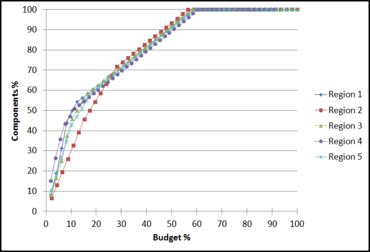
Because of experimental resource limitation, we have considered $5$ regions of Maricopa County for our experiments. We used IBM CPLEX Optimizer 12.5 to run the formulated ILP’s on the experimental dataset. We show our results in the figure 3. We observe that in each of the regions there is a specific budget threshold beyond which each additional increment in budget results in the death of only one entity. The reason for this behavior is our assumption that entities such as the transmission lines and the fiberlinks are not dependent on any other entities. We notice that all the entities of the two networks can be destroyed with a budget of about $60\%$ of the number of entities of the two networks $A$ and $B$ . Most importantly, we find that the degree of vulnerability of all the five regions considered in our study are close and no one region stands out as being extremely vulnerable.

References

[1] S. V. Buldyrev, R. Parshani, G. Paul, H. E. Stanley, and S. Havlin, “Catastrophic cascade of failures in interdependent networks,” Nature, vol. 464, no. 7291, pp. 1025–1028, 2010.
[2] J. Gao, S. V. Buldyrev, H. E. Stanley, and S. Havlin, “Networks formed from interdependent networks,” Nature Physics, vol. 8, no. 1, pp. 40–48, 2011.
[3] J. Shao, S. V. Buldyrev, S. Havlin, and H. E. Stanley, “Cascade of failures in coupled network systems with multiple support-dependence relations,” Physical Review E, vol. 83, no. 3, p. 036116, 2011.
[4] V. Rosato, L. Issacharoff, F. Tiriticco, S. Meloni, S. Porcellinis, and R. Setola, “Modelling interdependent infrastructures using interacting dynamical models,” International Journal of Critical Infrastructures, vol. 4, no. 1, pp. 63–79, 2008.
[5] P. Zhang, S. Peeta, and T. Friesz, “Dynamic game theoretic model of multi-layer infrastructure networks,” Networks and Spatial Economics, vol. 5, no. 2, pp. 147–178, 2005.
[6] M. Parandehgheibi and E. Modiano, “Robustness of interdependent networks: The case of communication networks and the power grid,” arXiv preprint arXiv:1304.0356, 2013.
[7] D. T. Nguyen, Y. Shen, and M. T. Thai, “Detecting critical nodes in interdependent power networks for vulnerability assessment,” 2013.
[8] A. Bernstein, D. Bienstock, D. Hay, M. Uzunoglu, and G. Zussman, “Power grid vulnerability to geographically correlated failures-analysis and control implications,” arXiv preprint arXiv:1206.1099, 2012.
[9] J.-F. Castet and J. H. Saleh, “Interdependent multi-layer networks: Modeling and survivability analysis with applications to space-based networks,” PloS one, vol. 8, no. 4, p. e60402, 2013.
[10] A. Fudenberg and J. Tirole, Game Theory. Ane Books, 2010.