跳到论文正文
W Papers独立论文阅读器 arXiv:1401.1519 论文正文 计算阅读时间 · 0%
引用这篇论文根据当前论文元数据生成,正式投稿前建议核对。


License: arXiv.org perpetual non-exclusive license
arXiv:1401.1519v1 [math.AP] 07 Jan 2014

Perturbations of the Dirichlet Problem and Error Bounds

Charles Z. Martin
August 24, 2026
Abstract

The Dirichlet problem on a bounded planar domain is more readily understood and solved for the Laplace operator than it is for a Schrödinger operator. When the potential function is small, we might hope to approximate the solution to the Schrödinger equation with the solution to the Laplace equation. In this vein we develop a series expansion for the solution and give explicit bounds on the error terms when truncating the series. We also examine a handful of examples and derive similar results for the Green function and Dirichlet–to–Neumann map.

1 Introduction

Consider a boundary value problem with Dirichlet data, in the form

{L​φ=0 in ​Dφ=f on ​∂D,\begin{cases}L\varphi=0&\textrm{ in }D\\ \varphi=f&\textrm{ on }\partial D,\end{cases} (1)

where LL is a second–order, linear, elliptic differential operator and DD is a bounded domain in the plane with sufficiently nice boundary. In trying to solve this problem, there are a few potential obstacles; the domain could be difficult to handle, the operator might be overly complicated, or—most commonly—a combination of the two. In this paper we discuss a method of approximating (1) that arises from viewing LL as a perturbation of the Laplacian and bound the resulting error. The approach is motivated as follows.

Suppose that L=LϵL=L_{\epsilon} denotes an elliptic operator depending on some perturbation parameter ϵ\epsilon, with L0=ΔL_{0}=\Delta. Let’s denote the solution to (1) by φϵ\varphi_{\epsilon}; the unperturbed solution is denoted φ0\varphi_{0}. These functions are identical on ∂D\partial D, so their difference satisfies

{Lϵ​(φϵ−φ0)=−Lϵ​φ0 in ​Dφϵ−φ0=0 on ​∂D.\begin{cases}L_{\epsilon}(\varphi_{\epsilon}-\varphi_{0})=-L_{\epsilon}\varphi_{0}&\textrm{ in }D\\ \varphi_{\epsilon}-\varphi_{0}=0&\textrm{ on }\partial D.\end{cases}

Since Lϵ≈ΔL_{\epsilon}\approx\Delta, we have −Lϵ​φ0-L_{\epsilon}\varphi_{0} is very small—in fact, it vanishes to zeroth order in ϵ\epsilon. What remains is an inhomogeneous problem with zero boundary data, which can be solved with knowledge of the Green function of LϵL_{\epsilon}. Thus we have reduced the problem of approximating φϵ\varphi_{\epsilon} to that of approximating a Green function. A well–known, classical formula due to Hadamard (see [1], for example) approximates the change in a Green function due to perturbations of the domain, but we’ll instead make use of a result approximating the change arising from operator variation, as detailed below.

Now let’s be more specific. Consider a Schrödinger operator L=Δ−ϵ​uL=\Delta-\epsilon u, where u≥0u\geq 0 is a smooth scalar function. Given a point w∈Dw\in D, the Green function gw∗g_{w}^{*} of LL is defined as the solution to

{L​gw∗=δw in ​Dgw∗=0 on ​∂D.\begin{cases}Lg^{*}_{w}=\delta_{w}&\textrm{ in }D\\ g^{*}_{w}=0&\textrm{ on }\partial D.\end{cases}

In the case ϵ=0\epsilon=0 we have L=ΔL=\Delta and denote the Green function simply by gwg_{w}. In other words, gw∗g^{*}_{w} is the perturbation of gwg_{w}. The following variational formula is derived, discussed and proved in [4].

Theorem 1.

Consider a bounded domain D⊂ℂD\subset\mathbb{C} with C1C^{1} boundary and let u∈C∞​(D¯)u\in C^{\infty}(\overline{D}). Fix w∈Dw\in D and define the integral operator

T​φ​(z)=∫Dφ​u​gz​𝑑A.T\varphi(z)=\int_{D}\varphi ug_{z}\,dA.

The Green function gw∗g_{w}^{*} of the Schrödinger operator Δ−ϵ​u\Delta-\epsilon u satisfies

gw∗=gw+ϵ​T​gw+o⁡(ϵ)g^{*}_{w}=g_{w}+\epsilon Tg_{w}+o(\epsilon)

as ϵ→0\epsilon\to 0, where the convergence of o⁡(ϵ)o(\epsilon) is uniform. Furthermore, a full series expansion is given by

gw∗=∑n=0∞ϵn​Tn​gw.g^{*}_{w}=\sum_{n=0}^{\infty}\epsilon^{n}T^{n}g_{w}. (2)

With this result we can turn to the approximation of solutions to the Dirichlet problem. Before that, however, we take a moment to discuss error bounds for the approximations of theorem 1.

2 Error Bounds for Variation of the Green Function

Although the first order correction given in theorem 1 is correct as ϵ→0\epsilon\to 0, practical computation might demand explicit error bounds for a fixed perturbation parameter. The rest of this section is devoted to the following theorem.

Theorem 2.

Let D⊂ℂD\subset\mathbb{C} be a bounded domain with C1C^{1} boundary and let u∈C∞​(D¯)u\in C^{\infty}(\overline{D}). For fixed w∈Dw\in D consider the Green function gw∗g^{*}_{w} of the operator Δ−ϵ​u\Delta-\epsilon u on the domain DD (with ϵ>0\epsilon>0). The remainder RnR_{n} in the expansion

gw∗=gw+ϵ​T​gw+⋯+ϵn−1​Tn−1​gw+Rng^{*}_{w}=g_{w}+\epsilon Tg_{w}+\cdots+\epsilon^{n-1}T^{n-1}g_{w}+R_{n}

is uniformly bounded by

‖Rn‖∞≤(ϵ​‖u‖∞​diam​(D)12)n​diam⁡(D)4​3​π.\|R_{n}\|_{\infty}\leq\left(\frac{\epsilon\|u\|_{\infty}\mathrm{diam}(D)}{\sqrt{12}}\right)^{n}\frac{\mathrm{diam}(D)}{4\sqrt{3\pi}}.

For simplicity, we often write |Rn||R_{n}| in place of ‖Rn‖∞\|R_{n}\|_{\infty}. Proof of this theorem requires bounding the tail of the series (2), ultimately reducing to easily–understood quantities such as the diameter of the domain. The following lemmas serve this purpose.

Lemma 3.

With the same assumptions as the previous theorem, given φ∈L2​(D)\varphi\in L^{2}(D) we have the pointwise bound |T​φ​(z)|≤‖u‖∞​‖gz‖2​‖φ‖2|T\varphi(z)|\leq\|u\|_{\infty}\|g_{z}\|_{2}\|\varphi\|_{2}. Furthermore, the operator norm of T:L2→L2T:L^{2}\to L^{2} satisfies

‖T‖≤‖u‖∞​(∫D‖gξ‖22​𝑑A​(ξ))1/2=‖u‖∞​(∬D2|g⁡(ξ,τ)|2​d​A2​(ξ,τ))1/2.\|T\|\leq\|u\|_{\infty}\left(\int_{D}\|g_{\xi}\|_{2}^{2}\,dA(\xi)\right)^{1/2}=\|u\|_{\infty}\left(\iint_{D^{2}}|g(\xi,\tau)|^{2}\,dA^{2}(\xi,\tau)\right)^{1/2}. (3)
Proof.

The Cauchy–Schwarz inequality gives

|T​φ​(ξ)|=|∫Du​gξ​φ​𝑑A|≤|u|∫D∞|gξ​φ|𝑑A≤‖u‖∞​‖gξ‖2​‖φ‖2.|T\varphi(\xi)|=\left|\int_{D}ug_{\xi}\varphi\,dA\right|\leq\|u\|_{\infty}\int_{D}|g_{\xi}\varphi|\,dA\leq\|u\|_{\infty}\|g_{\xi}\|_{2}\|\varphi\|_{2}.

Integrating |T​φ​(ξ)|2|T\varphi(\xi)|^{2} over DD yields

‖T​φ‖2≤‖u‖∞​‖φ‖2​(∫D‖gξ‖22​𝑑A​(ξ))1/2,\|T\varphi\|_{2}\leq\|u\|_{\infty}\|\varphi\|_{2}\left(\int_{D}\|g_{\xi}\|_{2}^{2}\,dA(\xi)\right)^{1/2},

from which the result follows. ∎

Lemma 4.

For z∈𝔻z\in\mathbb{D}, the Green function gzg_{z} of the Laplacian on 𝔻\mathbb{D} satisfies ∥gz∥2≤∥g0∥2=(8π)−1/2\|g_{z}\|_{2}\leq\|g_{0}\|_{2}=(8\pi)^{-1/2}.

Proof.

First note that ‖gz‖2\|g_{z}\|_{2} only depends upon r=|z|r=|z| and that ‖g1‖2=0\|g_{1}\|_{2}=0, so we need to consider the integral

∫𝔻ln2⁡|w−r1−r​w|​𝑑A​(w)\int_{\mathbb{D}}\ln^{2}\left|\frac{w-r}{1-rw}\right|\,dA(w)

when 0≤r<10\leq r<1. The substitution ξ=(w−r)/(1−r​w)\xi=(w-r)/(1-rw) preserves the unit disk, giving

∫𝔻ln2⁡|w−r1−r​w|​𝑑A​(w)=∫𝔻ln2⁡|ξ|​(1−r2)2|1+r​ξ|4​𝑑A​(ξ).\int_{\mathbb{D}}\ln^{2}\left|\frac{w-r}{1-rw}\right|\,dA(w)=\int_{\mathbb{D}}\ln^{2}|\xi|\frac{(1-r^{2})^{2}}{|1+r\xi|^{4}}\,dA(\xi).

Consider the difference ‖g0‖22−‖gz‖22\|g_{0}\|^{2}_{2}-\|g_{z}\|^{2}_{2} as follows:

‖g0‖22−‖gz‖22\displaystyle\|g_{0}\|^{2}_{2}-\|g_{z}\|^{2}_{2} =14​π2​∫𝔻ln2|ξ|(1−(1−r2)2|1+r​ξ|4)​𝑑A​(ξ)\displaystyle=\frac{1}{4\pi^{2}}\int_{\mathbb{D}}\ln^{2}|\xi|\left(1-\frac{(1-r^{2})^{2}}{|1+r\xi|^{4}}\right)\,dA(\xi)
≥14​π2​∫𝔻ln2|ξ|(1−(1−r2)21−r4​|ξ|4)​𝑑A​(ξ)\displaystyle\geq\frac{1}{4\pi^{2}}\int_{\mathbb{D}}\ln^{2}|\xi|\left(1-\frac{(1-r^{2})^{2}}{1-r^{4}|\xi|^{4}}\right)\,dA(\xi)
=14​π2​∫𝔻ln2|ξ|(2​r2−r4​(1+|ξ|4)1−r4​|ξ|4)​𝑑A​(ξ).\displaystyle=\frac{1}{4\pi^{2}}\int_{\mathbb{D}}\ln^{2}|\xi|\left(\frac{2r^{2}-r^{4}(1+|\xi|^{4})}{1-r^{4}|\xi|^{4}}\right)\,dA(\xi).

Since 0≤r<10\leq r<1 and ξ∈𝔻\xi\in\mathbb{D}, we have r4​(1+|ξ|4)≤2​r2r^{4}(1+|\xi|^{4})\leq 2r^{2} and the desired inequality follows. The computation of ‖g0‖2\|g_{0}\|_{2} is a standard exercise in polar coordinates. ∎

Lemma 5.

Let DD be as in theorem 1. Then for z∈Dz\in D we have the bounds

‖gz‖2≤diam⁡(D)24​π and (∬D2|g⁡(ξ,τ)|2​d​A2​(ξ,τ))1/2≤diam⁡(D)12.\displaystyle\|g_{z}\|_{2}\leq\frac{\mathrm{diam}(D)}{\sqrt{24\pi}}\quad\textrm{ and }\quad\left(\iint_{D^{2}}|g(\xi,\tau)|^{2}\,dA^{2}(\xi,\tau)\right)^{1/2}\leq\frac{\mathrm{diam}(D)}{\sqrt{12}}.
Proof.

First note that, by translation and dilation, the previous lemma can be generalized to a disk DRD_{R} of radius RR centered at p∈ℂp\in\mathbb{C}. In this case, we have that

‖gξ‖2≤‖gp‖2=R8​π\|g_{\xi}\|_{2}\leq\|g_{p}\|_{2}=\frac{R}{\sqrt{8\pi}}

for any ξ∈DR\xi\in D_{R}. For such a disk we have that

∬DR2|g⁡(ξ,τ)|2​d​A2​(ξ,τ)=∫DR‖gξ‖22​𝑑A​(ξ)≤∫DRR28​π​𝑑A=R24.\iint_{D_{R}^{2}}|g(\xi,\tau)|^{2}\,dA^{2}(\xi,\tau)=\int_{D_{R}}\|g_{\xi}\|_{2}^{2}\,dA(\xi)\leq\int_{D_{R}}\frac{R^{2}}{8\pi}\,dA=\frac{R^{2}}{4}.

Recall the monotonicity of the Green function as a domain functional: for Ω1⊆Ω2\Omega_{1}\subseteq\Omega_{2} we have

gΩ2≤gΩ1<0g_{\Omega_{2}}\leq g_{\Omega_{1}}<0

throughout Ω1\Omega_{1}. Thus if DD is contained within a disk of radius RR, we have

(∬D2|gD​(ξ,τ)|2​d​A2​(ξ,τ))1/2\displaystyle\left(\iint_{D^{2}}|g_{D}(\xi,\tau)|^{2}\,dA^{2}(\xi,\tau)\right)^{1/2} ≤(∬D2|gDR​(ξ,τ)|2​d​A2​(ξ,τ))1/2\displaystyle\leq\left(\iint_{D^{2}}|g_{D_{R}}(\xi,\tau)|^{2}\,dA^{2}(\xi,\tau)\right)^{1/2}
≤(∬DR2|gDR​(ξ,τ)|2​d​A2​(ξ,τ))1/2\displaystyle\leq\left(\iint_{{D_{R}}^{2}}|g_{D_{R}}(\xi,\tau)|^{2}\,dA^{2}(\xi,\tau)\right)^{1/2}
≤R2.\displaystyle\leq\frac{R}{2}.

The results follow from Jung’s theorem [3]: a domain of diameter dd is contained in a disk of radius d/3d/\sqrt{3}. ∎

Proof of Theorem 2.

We have that Rn=ϵn​(T)n​gw∗R_{n}=\epsilon^{n}(T)^{n}g^{*}_{w}. Lemma 3 gives

|Rn|≤ϵn​‖u‖∞​‖gw‖2​‖Tn−1​gw∗‖2≤ϵn​‖u‖∞​‖gw‖2​‖T‖n−1​‖gw∗‖2.|R_{n}|\leq\epsilon^{n}\|u\|_{\infty}\|g_{w}\|_{2}\|T^{n-1}g_{w}^{*}\|_{2}\leq\epsilon^{n}\|u\|_{\infty}\|g_{w}\|_{2}\|T\|^{n-1}\|g_{w}^{*}\|_{2}.

Note that theorem 1 implies that gw≤gw∗≤0g_{w}\leq g_{w}^{*}\leq 0, and hence ‖gw∗‖2≤‖g2‖2\|g_{w}^{*}\|_{2}\leq\|g_{2}\|_{2}. With lemmas 3 and 5 we obtain

|Rn|≤ϵn​‖u‖∞​(diam⁡(D)24​π)2​(‖u‖∞​diam⁡(D)12)n−1|R_{n}|\leq\epsilon^{n}\|u\|_{\infty}\left(\frac{\mathrm{diam}(D)}{\sqrt{24\pi}}\right)^{2}\left(\|u\|_{\infty}\frac{\mathrm{diam}(D)}{\sqrt{12}}\right)^{n-1}

which rearranges into the result. ∎

Example 6.

Consider the problem of estimating the Green function gw∗g_{w}^{*} of Δ−1\Delta-1 on the unit disk 𝔻\mathbb{D}. Viewing Δ−1\Delta-1 as a perturbation of Δ\Delta gives

gw∗​(z)=gw​(z)+∫𝔻gz​gw​𝑑A+R2​(z),g_{w}^{*}(z)=g_{w}(z)+\int_{\mathbb{D}}g_{z}g_{w}\,dA+R_{2}(z), (4)

with R2R_{2} bounded by

|R2|≤16​π​3≃0.0306.|R_{2}|\leq\frac{1}{6\pi\sqrt{3}}\simeq 0.0306. (5)

We can evaluate the integral in (4) as follows. Note that gw​gz=∂n(gw​gz)=0g_{w}g_{z}=\partial_{n}(g_{w}g_{z})=0 on ∂𝔻\partial\mathbb{D}, so we have that

∫𝔻gz​gw​𝑑A\displaystyle\int_{\mathbb{D}}g_{z}g_{w}\,dA =∫𝔻gw​(ξ)​gz​(ξ)​Δ​(|ξ|24)​𝑑A​(ξ)\displaystyle=\int_{\mathbb{D}}g_{w}(\xi)g_{z}(\xi)\Delta\left(\frac{|\xi|^{2}}{4}\right)\,dA(\xi)
=∫𝔻|ξ|24​Δ​(gz​(ξ)​gw​(ξ))​𝑑A​(ξ)\displaystyle=\int_{\mathbb{D}}\frac{|\xi|^{2}}{4}\Delta(g_{z}(\xi)g_{w}(\xi))\,dA(\xi)
=14∫𝔻|ξ|2(gzδw+gwδz)dA(ξ)+12∫𝔻|ξ|2∇gz(ξ)⋅∇gw(ξ)dA(ξ)\displaystyle=\frac{1}{4}\int_{\mathbb{D}}|\xi|^{2}(g_{z}\delta_{w}+g_{w}\delta_{z})\,dA(\xi)+\frac{1}{2}\int_{\mathbb{D}}|\xi|^{2}\nabla g_{z}(\xi)\cdot\nabla g_{w}(\xi)\,dA(\xi)
=gw(z)(|z|2+|w|24)+12∫𝔻|ξ|2∇gz(ξ)⋅∇gw(ξ)dA(ξ).\displaystyle=g_{w}(z)\left(\frac{|z|^{2}+|w|^{2}}{4}\right)+\frac{1}{2}\int_{\mathbb{D}}|\xi|^{2}\nabla g_{z}(\xi)\cdot\nabla g_{w}(\xi)\,dA(\xi).

This last integral was evaluated in the final example of [4]; when z​w≠0zw\neq 0 the result is

∫𝔻gz​gw​𝑑A=gw​(z)​(|z|2+|w|24)+18​π​Re​[(z​w¯+z¯w¯+wz−1z​w¯)​log⁡(1−z​w¯)−2​z​w¯​log⁡|z−w|]\int_{\mathbb{D}}g_{z}g_{w}\,dA=g_{w}(z)\left(\frac{|z|^{2}+|w|^{2}}{4}\right)+\frac{1}{8\pi}\mathrm{Re}\,\left[\left(z\overline{w}+\frac{\overline{z}}{\overline{w}}+\frac{w}{z}-\frac{1}{z\overline{w}}\right)\log(1-z\overline{w})-2z\overline{w}\log|z-w|\right]

When w=0w=0 we instead have

∫𝔻gz​g0​𝑑A=1−|z|2​(1−log⁡|z|)8​π.\int_{\mathbb{D}}g_{z}g_{0}\,dA=\frac{1-|z|^{2}(1-\log|z|)}{8\pi}.

As a comparison, the actual Green function with singularity at 0 is given by

g0∗​(z)=K0​(1)−K0​(|z|)2​π,g_{0}^{*}(z)=\frac{K_{0}(1)-K_{0}(|z|)}{2\pi},

where K0K_{0} denotes the modified Bessel function of the second kind. The error R2​(z)R_{2}(z) is given by

R2​(z)=K0​(1)−K0​(|z|)2​π−log⁡|z|2​π−1−|z|2​(1−log⁡|z|)8​π,R_{2}(z)=\frac{K_{0}(1)-K_{0}(|z|)}{2\pi}-\frac{\log|z|}{2\pi}-\frac{1-|z|^{2}(1-\log|z|)}{8\pi}, (6)

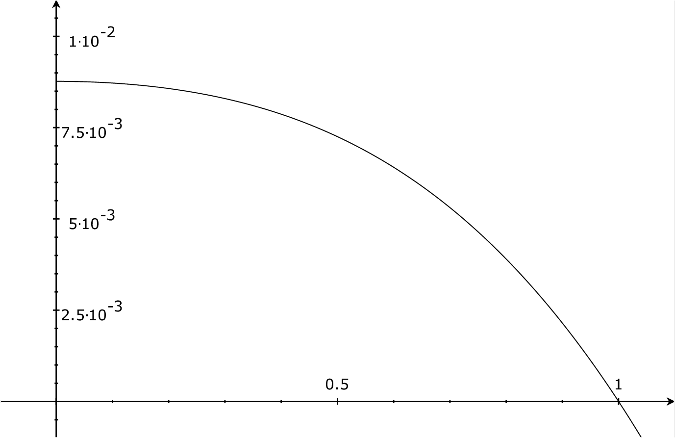
which takes values in the interval [0,0.0088][0,0.0088], confirming error bound (5). A basic plot of R2R_{2} is shown in figure 1.

Refer to caption
Figure 1: A plot of R2​(|z|)R_{2}(|z|), as given in equation (6).

3 Application to Boundary–Value Problems

3.1 Variation of the Dirichlet Problem

Consider solving the Dirichlet problem on a domain DD:

{(Δ−ϵ​u)​φϵ=0 in ​Dφϵ=f on ​∂D\begin{cases}(\Delta-\epsilon u)\varphi_{\epsilon}=0&\textrm{ in }D\\ \varphi_{\epsilon}=f&\textrm{ on }\partial D\end{cases} (7)

where ff is a bounded Borel function, u≥0u\geq 0 is smooth in a neighborhood of D¯\overline{D} and ϵ≥0\epsilon\geq 0 is small. If we ignored the ϵ​u\epsilon u term in the problem—that is, assume ϵ\epsilon is zero—we can estimate the error with the following theorem and corollary.

Theorem 7.

Let D⊂ℂD\subset\mathbb{C} be a bounded domain with C1C^{1} boundary and suppose u∈C∞​(D¯)u\in C^{\infty}(\overline{D}) is a positive function. For ϵ≥0\epsilon\geq 0 and a bounded Borel function ff the solution φϵ\varphi_{\epsilon} to the Dirichlet problem (7) satisfies

φϵ​(z)=φ0​(z)+ϵ​∫Du​φ0​gz​𝑑A+o⁡(ϵ)\varphi_{\epsilon}(z)=\varphi_{0}(z)+\epsilon\int_{D}u\varphi_{0}g_{z}\,dA+o(\epsilon)

as ϵ→0\epsilon\to 0, where the error term converges uniformly in zz. Using the notation of theorem 1, a full series expansion is given by

φϵ​(z)=∑n=0∞ϵn​Tn​φ0.\varphi_{\epsilon}(z)=\sum_{n=0}^{\infty}\epsilon^{n}T^{n}\varphi_{0}. (8)
Proof.

Let gw∗g^{*}_{w} denote the Green function of the operator Δ−ϵ​u\Delta-\epsilon u in the region DD. Note that

{(Δ−ϵ​u)​(φϵ−φ0)=ϵ​u​φ0 in ​Dφϵ−φ0=0 on ​∂D,\begin{cases}(\Delta-\epsilon u)(\varphi_{\epsilon}-\varphi_{0})=\epsilon u\varphi_{0}&\textrm{ in }D\\ \varphi_{\epsilon}-\varphi_{0}=0&\textrm{ on }\partial D,\end{cases}

whence an expression for φϵ\varphi_{\epsilon} is given by

φϵ​(z)=φ0​(z)+ϵ​∫Du​φ0​gz∗​𝑑A.\varphi_{\epsilon}(z)=\varphi_{0}(z)+\epsilon\int_{D}u\varphi_{0}g^{*}_{z}\,dA.

From the perturbation formula (8) we have

φϵ​(z)=φ0​(z)+ϵ​∫Du​φ0​gz​𝑑A+o⁡(ϵ),\varphi_{\epsilon}(z)=\varphi_{0}(z)+\epsilon\int_{D}u\varphi_{0}g_{z}\,dA+o(\epsilon),

as desired. The full series expansion follows from instead using the full series given in theorem 1. ∎

Corollary 8.

With the same assumptions as the previous theorem, the linearization of φϵ\varphi_{\epsilon} has the pointwise bound

|δ​φϵ​(z)|≤‖u‖2​‖gz‖2​‖f‖∞.|\delta\varphi_{\epsilon}(z)|\leq\|u\|_{2}\|g_{z}\|_{2}\|f\|_{\infty}.
Proof.

From the maximum modulus principle for harmonic functions, supD|φ0|≤sup∂D|f|\sup_{D}|\varphi_{0}|\leq\sup_{\partial D}|f|. The result follows from this and the Cauchy-Schwarz inequality. ∎

The following lemma aids computation of simple examples in the disk.

Lemma 9.

Given a point z∈𝔻z\in\mathbb{D} and an integer n≥0n\geq 0 we have

∫𝔻|ξ|2​n​gz​(ξ)​𝑑A​(ξ)=−1−|z|2​n+24​(n+1)2,\int_{\mathbb{D}}|\xi|^{2n}g_{z}(\xi)\,dA(\xi)=-\frac{1-|z|^{2n+2}}{4(n+1)^{2}},

where gzg_{z} denotes the Green function of the Laplacian on 𝔻\mathbb{D} with singularity at zz.

Proof.

First we note that

Δ⁡(|ξ|2​n+24​(n+1)2)=4​∂∂¯​((ξ​ξ¯)n+14​(n+1)2)=|ξ|2​n.\Delta\left(\frac{|\xi|^{2n+2}}{4(n+1)^{2}}\right)=4\partial\overline{\partial}\left(\frac{(\xi\overline{\xi})^{n+1}}{4(n+1)^{2}}\right)=|\xi|^{2n}.

We use the Poisson–Jensen formula

v⁡(z)=∫∂𝔻v​∂ngz​𝑑s+∫𝔻gz​Δ​v​𝑑Av(z)=\int_{\partial\mathbb{D}}v\partial_{n}g_{z}\,ds+\int_{\mathbb{D}}g_{z}\Delta v\,dA

to write

|z|2​n+24​(n+1)2\displaystyle\frac{|z|^{2n+2}}{4(n+1)^{2}} =∫∂𝔻|ζ|2​n+24​(n+1)2​∂ngz​(ζ)​𝑑s​(ζ)+∫𝔻|ξ|2​n​gz​(ξ)​𝑑A​(ξ)\displaystyle=\int_{\partial\mathbb{D}}\frac{|\zeta|^{2n+2}}{4(n+1)^{2}}\partial_{n}g_{z}(\zeta)ds(\zeta)+\int_{\mathbb{D}}|\xi|^{2n}g_{z}(\xi)\,dA(\xi)
=∫∂𝔻∂ngz4​(n+1)2​𝑑s+∫𝔻|ξ|2​n​gz​(ξ)​𝑑A​(ξ)\displaystyle=\int_{\partial\mathbb{D}}\frac{\partial_{n}g_{z}}{4(n+1)^{2}}\,ds+\int_{\mathbb{D}}|\xi|^{2n}g_{z}(\xi)\,dA(\xi)
=14​(n+1)2+∫𝔻|ξ|2​n​gz​(ξ)​𝑑A​(ξ),\displaystyle=\frac{1}{4(n+1)^{2}}+\int_{\mathbb{D}}|\xi|^{2n}g_{z}(\xi)\,dA(\xi),

where we’ve used the facts that |ζ|=1|\zeta|=1 on ∂𝔻\partial\mathbb{D} and that ∂ngz​d​s\partial_{n}g_{z}\,ds is a probability measure on ∂𝔻\partial\mathbb{D}. We conclude that

∫𝔻|ξ|2​n​gz​(ξ)​𝑑A​(ξ)=−1−|z|2​n+24​(n+1)2,\int_{\mathbb{D}}|\xi|^{2n}g_{z}(\xi)\,dA(\xi)=-\frac{1-|z|^{2n+2}}{4(n+1)^{2}},

as desired. ∎

Example 10.

For a simple example, consider the Dirichlet problem for the Helmholtz equation on the unit disk 𝔻\mathbb{D}:

{(Δ−a)​φa=0 in ​𝔻φa=1 on ​∂𝔻,\begin{cases}(\Delta-a)\varphi_{a}=0&\textrm{ in }\mathbb{D}\\ \varphi_{a}=1&\textrm{ on }\partial\mathbb{D},\end{cases}

where 0<a≪10<a\ll 1. Clearly φ0≡1\varphi_{0}\equiv 1, so we obtain

φa​(z)=1+a​∫𝔻gz​𝑑A+o⁡(a),\varphi_{a}(z)=1+a\int_{\mathbb{D}}g_{z}\,dA+o(a), (9)

where the Green function gzg_{z} is given by

gz​(ξ)=12​π​ln⁡|ξ−z1−z¯​ξ|.g_{z}(\xi)=\frac{1}{2\pi}\ln\left|\frac{\xi-z}{1-\overline{z}\xi}\right|.

Lemma 9 gives

∫𝔻gz​𝑑A​(ξ)=−1−|z|24,\int_{\mathbb{D}}g_{z}\,dA(\xi)=-\frac{1-|z|^{2}}{4},

so equation (9) becomes

φa​(z)=1−a4​(1−|z|2)+o⁡(a).\varphi_{a}(z)=1-\frac{a}{4}(1-|z|^{2})+o(a).

3.2 Explicit Error Bounds

In this section we prove an analogue to theorem 2 for the perturbation of the Dirichlet problem considered above. Afterwards, we discuss a few examples to illustrate the approach’s strengths and shortcomings.

Theorem 11.

Let D⊂ℂD\subset\mathbb{C} be a bounded domain with C1C^{1} boundary and suppose u∈C∞​(D¯)u\in C^{\infty}(\overline{D}) is a positive function. For ϵ≥0\epsilon\geq 0 and a bounded Borel function ff we can write the solution φϵ\varphi_{\epsilon} to the Dirichlet problem (7) as

φϵ​(z)=φ0​(z)+ϵ​T​φ0+⋯+ϵn−1​Tn−1​φ0+Rn​(z),\varphi_{\epsilon}(z)=\varphi_{0}(z)+\epsilon T\varphi_{0}+\cdots+\epsilon^{n-1}T^{n-1}\varphi_{0}+R_{n}(z),

where TT is as defined in theorem 1. A uniform bound for the error RnR_{n} is given by

‖Rn‖∞≤(ϵ​‖u‖∞​diam​(D)12)n​‖f‖∞​area⁡(D)2​π.\|R_{n}\|_{\infty}\leq\left(\frac{\epsilon\|u\|_{\infty}\mathrm{diam}(D)}{\sqrt{12}}\right)^{n}\frac{\|f\|_{\infty}\sqrt{\mathrm{area}(D)}}{\sqrt{2\pi}}.
Proof.

From theorem 7 we have that

Rn​(z)=ϵn​Tn​φϵ​(z).R_{n}(z)=\epsilon^{n}T^{n}\varphi_{\epsilon}(z).

Using the pointwise bound in lemma 3 gives

|Rn​(z)|\displaystyle|R_{n}(z)| ≤ϵn​‖Tn​φϵ‖∞\displaystyle\leq\epsilon^{n}\|T^{n}\varphi_{\epsilon}\|_{\infty}
≤ϵn​‖u‖∞​‖Tn−1​φϵ‖2​supz‖gz‖2\displaystyle\leq\epsilon^{n}\|u\|_{\infty}\|T^{n-1}\varphi_{\epsilon}\|_{2}\sup_{z}\|g_{z}\|_{2}
≤ϵn​‖u‖∞​‖T‖n−1​‖φϵ‖2​supz‖gz‖2.\displaystyle\leq\epsilon^{n}\|u\|_{\infty}\|T\|^{n-1}\|\varphi_{\epsilon}\|_{2}\sup_{z}\|g_{z}\|_{2}.

Lemmas 3 and 5 also yield

‖T‖≤‖u‖∞​(∬D2|g⁡(ξ,τ)|2​d​A2​(ξ,τ))1/2≤‖u‖∞​diam​(D)12.\|T\|\leq\|u\|_{\infty}\left(\iint_{D^{2}}|g(\xi,\tau)|^{2}\,dA^{2}(\xi,\tau)\right)^{1/2}\leq\frac{\|u\|_{\infty}\mathrm{diam}(D)}{\sqrt{12}}.

Together with the bound on ‖gz‖2\|g_{z}\|_{2} in lemma 5 we have

|Rn​(z)|\displaystyle|R_{n}(z)| ≤(ϵ​‖u‖∞​diam​(D)12)n​‖φϵ‖22​π\displaystyle\leq\left(\frac{\epsilon\|u\|_{\infty}\mathrm{diam}(D)}{\sqrt{12}}\right)^{n}\frac{\|\varphi_{\epsilon}\|_{2}}{\sqrt{2\pi}}
≤(ϵ​‖u‖∞​diam​(D)12)n​‖φ0‖∞​area⁡(D)2​π.\displaystyle\leq\left(\frac{\epsilon\|u\|_{\infty}\mathrm{diam}(D)}{\sqrt{12}}\right)^{n}\frac{\|\varphi_{0}\|_{\infty}\sqrt{\mathrm{area}(D)}}{\sqrt{2\pi}}.

The result follows from the maximum principle for Δ−ϵ​u\Delta-\epsilon u; that is, ‖φϵ‖∞≤‖f‖∞\|\varphi_{\epsilon}\|_{\infty}\leq\|f\|_{\infty}. ∎

Corollary 12.

In the case when DD is a disk of radius rr the error bounds can be tightened into

‖Rn‖∞≤(ϵ​r​‖u‖∞2)n​r​‖f‖∞2.\|R_{n}\|_{\infty}\leq\left(\frac{\epsilon r\|u\|_{\infty}}{2}\right)^{n}\frac{r\|f\|_{\infty}}{\sqrt{2}}.
Example 13.

We return to the simple case of the previous example, the Dirichlet problem

{(Δ−a)​φa=0 in ​𝔻φa=1 on ​∂𝔻.\begin{cases}(\Delta-a)\varphi_{a}=0&\textrm{ in }\mathbb{D}\\ \varphi_{a}=1&\textrm{ on }\partial\mathbb{D}.\end{cases}

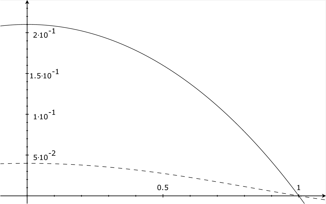
If we take a=1a=1 the solution is known to be φ1​(z)=I0​(|z|)/I0​(1)\varphi_{1}(z)=I_{0}(|z|)/I_{0}(1), where I0I_{0} denotes the zeroth order modified Bessel function of the first kind. The function φ1\varphi_{1} is an increasing function of |z||z|, and takes values in the interval [0.789,1][0.789,1]. Using corollary 12, the zeroth order approximation φ1​(z)≃φ0​(z)≡1\varphi_{1}(z)\simeq\varphi_{0}(z)\equiv 1 has error bounded by

|φ1−1|=|R1|≤(ϵ​r​‖u‖∞2)n​r​‖f‖∞2=18≃0.354.|\varphi_{1}-1|=|R_{1}|\leq\left(\frac{\epsilon r\|u\|_{\infty}}{2}\right)^{n}\frac{r\|f\|_{\infty}}{\sqrt{2}}=\frac{1}{\sqrt{8}}\simeq 0.354.

The actual error is

R1​(x)=1−I0​(x)I0​(1),R_{1}(x)=1-\frac{I_{0}(x)}{I_{0}(1)},

a plot of which appears in figure 2. The first order approximation is computed in the previous example as

φ1​(z)≃1−1−|z|24,\varphi_{1}(z)\simeq 1-\frac{1-|z|^{2}}{4},

with an error bound of

|R2|≤14​2≃0.177.|R_{2}|\leq\frac{1}{4\sqrt{2}}\simeq 0.177.

Indeed, R2​(z)=φ1​(z)−(1−1−|z|24)R_{2}(z)=\varphi_{1}(z)-(1-\frac{1-|z|^{2}}{4}) takes values in the interval [0,0.0399][0,0.0399], as seen in figure 2. Taking it one step further, we can use lemma 9 to compute the next order term:

φ1​(z)≃1−1−|z|24−G⁡(1−|z|24)=1−1−|z|24+|z|4−4​|z|2+364.\varphi_{1}(z)\simeq 1-\frac{1-|z|^{2}}{4}-G\left(\frac{1-|z|^{2}}{4}\right)=1-\frac{1-|z|^{2}}{4}+\frac{|z|^{4}-4|z|^{2}+3}{64}.

The estimated error is

|R3|≤18​2≃0.0884,|R_{3}|\leq\frac{1}{8\sqrt{2}}\simeq 0.0884,

though the real error is bounded by 0.00710.0071 (we chose not to plot R3R_{3} alongside the other error functions for visibility reasons). Even though the error bound decreases geometrically, it is far from tight in these first few cases.
Refer to caption
Figure 2: A plot of R1​(|z|)R_{1}(|z|) and R2​(|z|)R_{2}(|z|) from example 13. The solid line depicts R1R_{1}.
Example 14.

Continuing in a similar fashion to the previous example, consider the Dirichlet problem

{(Δ−ϵ​|z|2)​φϵ=0 in ​𝔻φϵ=1 on ​∂𝔻.\begin{cases}(\Delta-\epsilon|z|^{2})\varphi_{\epsilon}=0&\textrm{ in }\mathbb{D}\\ \varphi_{\epsilon}=1&\textrm{ on }\partial\mathbb{D}.\end{cases}

The solution to this problem when ϵ=1\epsilon=1 is φ1​(z)=I0​(|z|2/2)/I0​(1/2)\varphi_{1}(z)=I_{0}(|z|^{2}/2)/I_{0}(1/2). In particular, φ1​(𝔻)⊆[0.94,1]\varphi_{1}(\mathbb{D})\subseteq[0.94,1], which is a smaller range than before. In this situation the error in approximating φ1\varphi_{1} by φ0≡1\varphi_{0}\equiv 1 is less than 0.60.6; without this knowledge, the bound of corollary 12 gives

|φ1−1|=|R1|≤12​2≃0.354,|\varphi_{1}-1|=|R_{1}|\leq\frac{1}{2\sqrt{2}}\simeq 0.354,

the same bound as in the previous example. Unfortunately, theorem 11 cannot detect that Δ−|z|2\Delta-|z|^{2} is in some sense closer to Δ\Delta than Δ−1\Delta-1 is. This is due to the fact that ‖|z|2‖∞=‖1‖∞=1\||z|^{2}\|_{\infty}=\|1\|_{\infty}=1 on 𝔻\mathbb{D}.

Example 15.

For a less trivial example we turn to the Helmholtz operator on an ellipse of small eccentricity. Consider the Dirichlet problem

{(Δ−a)​φa=0 in ​Eφa=1 on ​∂E\begin{cases}(\Delta-a)\varphi_{a}=0&\textrm{ in }E\\ \varphi_{a}=1&\textrm{ on }\partial E\end{cases}

on the ellipse EE given by

x2+y21.12≤1.x^{2}+\frac{y^{2}}{1.1^{2}}\leq 1.

Here we use the standard identification z=x+i​yz=x+iy, with x,y∈ℝx,y\in\mathbb{R}. Once again note that φ0≡1\varphi_{0}\equiv 1 and that φ1​(z)≃1\varphi_{1}(z)\simeq 1 with error bounded by

|φ1−1|=|R1|≤2.2​1.124≃0.471.|\varphi_{1}-1|=|R_{1}|\leq\frac{2.2\sqrt{1.1}}{\sqrt{24}}\simeq 0.471.

In particular, 0.529≤φ⁡(0,0)≤10.529\leq\varphi(0,0)\leq 1. To compute the next order approximation, we have the following lemma.

Lemma 16.

For the elliptical region EE given by x2/a2+y2/b2≤1x^{2}/a^{2}+y^{2}/b^{2}\leq 1 and a point w=u+i​v∈Ew=u+iv\in E we have

∫Egw​𝑑A=(b​u)2+(a​v)2−(a​b)22​(a2+b2),\int_{E}g_{w}\,dA=\frac{(bu)^{2}+(av)^{2}-(ab)^{2}}{2(a^{2}+b^{2})},

where gwg_{w} denotes the Green function of the Laplacian on EE.

Proof.

Since both gwg_{w} and x2/a2+y2/b2−1x^{2}/a^{2}+y^{2}/b^{2}-1 vanish on ∂E\partial E, Green’s identity gives

(2a2+2b2)​∫Egw​𝑑A\displaystyle\left(\frac{2}{a^{2}}+\frac{2}{b^{2}}\right)\int_{E}g_{w}\,dA =∫Egw​(x,y)​Δ​(x2a2+y2b2−1)​𝑑A​(x,y)\displaystyle=\int_{E}g_{w}(x,y)\Delta\left(\frac{x^{2}}{a^{2}}+\frac{y^{2}}{b^{2}}-1\right)\,dA(x,y)
=∫E(x2a2+y2b2−1)​Δ​gw​(x,y)​𝑑A​(x,y)\displaystyle=\int_{E}\left(\frac{x^{2}}{a^{2}}+\frac{y^{2}}{b^{2}}-1\right)\Delta g_{w}(x,y)\,dA(x,y)
=u2a2+v2b2−1.∎\displaystyle=\frac{u^{2}}{a^{2}}+\frac{v^{2}}{b^{2}}-1.\qed

With lemma in hand we can compute

φ1​(x,y)=1+G​1+R2=1+1.21​x2+y2−1.214.42+R2​(x,y),\varphi_{1}(x,y)=1+G1+R_{2}=1+\frac{1.21x^{2}+y^{2}-1.21}{4.42}+R_{2}(x,y),

with R2R_{2} bounded by

|R2|≤2.22​1.112​2≃0.299.|R_{2}|\leq\frac{2.2^{2}\sqrt{1.1}}{12\sqrt{2}}\simeq 0.299.

In particular, 0.427≤φ⁡(0,0)≤10.427\leq\varphi(0,0)\leq 1. At the origin, our approximation gives a weaker bound than the one deduced from the first approximation.

4 The Dirichlet–to–Neumann Map

The Dirichlet–to–Neumann map Λu:H1/2(∂D)→H−1/2(∂D)\Lambda_{u}:H^{1/2}(\partial D)\to H^{-1/2}(\partial D) is defined by Λu​(f)=∂nφ\Lambda_{u}(f)=\partial_{n}\varphi, where φ\varphi solves the Dirichlet problem

{(Δ−u)​φ=0 in ​Dφ=f on ​∂D.\begin{cases}(\Delta-u)\varphi=0&\textrm{ in }D\\ \varphi=f&\textrm{ on }\partial D.\end{cases}

In practical applications the Dirichlet–to–Neumann map is readily determined via boundary measurements at ∂D\partial D. For this reason, there is much interest in inverse problems of the following type: given Λu\Lambda_{u}, can we determine uu? Traditionally more attention is paid to the Laplace–Beltrami inverse problem—that is, determine λ\lambda from knowledge of the Dirichlet–to–Neumann map of ∇λ∇\nabla\lambda\nabla. We will restrict our attention to the Schrödinger operator, as an application of the theorems in the previous sections.

In his brief but seminal work on the topic [2], A. P. Calderón considers the quadratic form arising from the self–adjoint operator Λ\Lambda, computes its linearization, and shows that the resulting linear map is injective. In a similar spirit we can compute the linearization of Λ\Lambda using theorem 7. We’ll make use of the following lemma, which is proved in [5].

Lemma 17.

Let DD be a bounded domain in ℂ\mathbb{C} with smooth, analytic boundary and suppose that f∈C1​(D¯)∩C2​(D)f\in C^{1}(\overline{D})\cap C^{2}(D). If f=0f=0 on ∂D\partial D then for ζ∈∂D\zeta\in\partial D,

∂f∂n​(ζ)=∫DPζ​Δ​f​𝑑A,\frac{\partial f}{\partial n}(\zeta)=\int_{D}P_{\zeta}\Delta f\,dA,

where Pζ​(z)=∂ngz​(ζ)P_{\zeta}(z)=\partial_{n}g_{z}(\zeta) is the Poisson kernel of DD.

With this lemma we can derive an expression for the Dirichlet–to–Neumann map for Δ−ϵ​u\Delta-\epsilon u. For given Dirichlet boundary data ff, define φϵ\varphi_{\epsilon} as the solution to the problem

{(Δ−ϵ​u)​φ=0 in ​Dφ=f on ​∂D.\begin{cases}(\Delta-\epsilon u)\varphi=0&\textrm{ in }D\\ \varphi=f&\textrm{ on }\partial D.\end{cases}

Note that φ0\varphi_{0} is the solution to the problem for the Laplace operator.

Theorem 18.

For a bounded domain D⊂ℂD\subset\mathbb{C} with smooth, analytic boundary we have

(Λϵ​u​f)​(ζ)=(Λ0​f)​(ζ)+ϵ​∫Du​Pζ​φ0​𝑑A+o⁡(ϵ).(\Lambda_{\epsilon u}f)(\zeta)=(\Lambda_{0}f)(\zeta)+\epsilon\int_{D}uP_{\zeta}\varphi_{0}\,dA+o(\epsilon).

An alternative expression is given by

(Λϵ​u​f)​(ζ)=(Λ0​f)​(ζ)+ϵ​∫∂Df⁡(ξ)​(∫Du​Pξ​Pζ​𝑑A)​𝑑s​(ξ)+o⁡(ϵ).(\Lambda_{\epsilon u}f)(\zeta)=(\Lambda_{0}f)(\zeta)+\epsilon\int_{\partial D}f(\xi)\left(\int_{D}uP_{\xi}P_{\zeta}\,dA\right)\,ds(\xi)+o(\epsilon).
Proof.

Note that φϵ−φ0\varphi_{\epsilon}-\varphi_{0} vanishes on ∂D\partial D. The lemma above gives

(Λϵ​u​f)​(ζ)−(Λ0​f)​(ζ)=∂n(φϵ−φ0)​(ζ)=∫DPζ​Δ​(φϵ−φ0)​𝑑A=∫Du​Pζ​φϵ​𝑑A.(\Lambda_{\epsilon u}f)(\zeta)-(\Lambda_{0}f)(\zeta)=\partial_{n}(\varphi_{\epsilon}-\varphi_{0})(\zeta)=\int_{D}P_{\zeta}\Delta(\varphi_{\epsilon}-\varphi_{0})\,dA=\int_{D}uP_{\zeta}\varphi_{\epsilon}\,dA.

Since φϵ=φ0+o⁡(ϵ)\varphi_{\epsilon}=\varphi_{0}+o(\epsilon), we obtain

(Λϵ​u​f)​(ζ)=(Λ0​f)​(ζ)+ϵ​∫Du​Pζ​φ0​𝑑A+o⁡(ϵ).(\Lambda_{\epsilon u}f)(\zeta)=(\Lambda_{0}f)(\zeta)+\epsilon\int_{D}uP_{\zeta}\varphi_{0}\,dA+o(\epsilon).

Finally, note that φ0\varphi_{0} can be written as a Poisson integral; this gives

∫Du​Pζ​φ0​𝑑A=∫Du⁡(τ)​Pζ​(τ)​(∫∂DPξ​(τ)​f​(ξ)​𝑑s​(ξ))​𝑑A​(τ)=∫∂Df⁡(ξ)​(∫Du​Pξ​Pζ​𝑑A)​𝑑s​(ξ).∎\int_{D}uP_{\zeta}\varphi_{0}\,dA=\int_{D}u(\tau)P_{\zeta}(\tau)\left(\int_{\partial D}P_{\xi}(\tau)f(\xi)\,ds(\xi)\right)\,dA(\tau)=\int_{\partial D}f(\xi)\left(\int_{D}uP_{\xi}P_{\zeta}\,dA\right)\,ds(\xi).\qed

References

  • [1] P. R. Garabedian, Partial Differential Equations, Chelsea, New York 1986.
  • [2] A. P. Calderón, On an inverse boundary value problem, Seminar on Numerical Analysis and its Applications to Continuum Physics, Soc. Brasileira de Matematica, Rio de Janeiro 1980.
  • [3] H. W. E. Jung, Über die kleinste Kugel, die eine räumliche Figur einschliesst, J. Reine Angew. Math. 123 (1901), 241–257.
  • [4] C. Z. Martin, Variational formulas for the Green function, Anal. Math. Phys. 2 (2012), 89–103.
  • [5] C. Z. Martin, Variation of normal derivatives of Green functions, J. Math. Anal. Appl. 401 (2013), 47–54.

Department of Mathematics, Vanderbilt University, Nashville, TN, 37240
charles.z.martin@vanderbilt.edu