Optical conductivity of a two-dimensional metal
at the onset of spin-density-wave order

Andrey V. Chubukov^a), Dmitrii L. Maslov^b), and Vladimir I. Yudson^c) Affiliation: ^a)Department of Physics, University of Wisconsin-Madison, 1150 Univ. Ave., Madison, WI 53706-1390
^b)Department of Physics, University of Florida, P. O. Box 118440, Gainesville, FL 32611-8440
^c)Institute for Spectroscopy, Russian Academy of Sciences, Troitsk, Moscow region, 142190, Russia

August 24, 2026

Abstract

We consider the optical conductivity of a clean two-dimensional metal near a quantum spin-density-wave transition. Critical magnetic fluctuations are known to destroy fermionic coherence at “hot spots” of the Fermi surface but coherent quasiparticles survive in the rest of the Fermi surface. A large part of the Fermi surface is not really “cold” but rather “lukewarm” in a sense that coherent quasiparticles in that part survive

but are strongly renormalized compared to the non-interacting case. We discuss the self-energy of lukewarm fermions and their contribution to the optical conductivity, $\sigma(\Omega)$ , focusing specifically on scattering off composite bosons made of two critical magnetic fluctuations. Recent study [S.A. Hartnoll et al., Phys. Rev. B 84, 125115 (2011)] found that composite scattering gives the strongest contribution to the self-energy of lukewarm fermions and suggested that this may give rise to a non-Fermi liquid behavior of the optical conductivity at the lowest frequencies. We show that the most singular term in the conductivity coming from self-energy insertions into the conductivity bubble, $\sigma^{\prime}(\Omega)\propto\ln^{3}\Omega/\Omega^{1/3}$ , is canceled out by the vertex-correction and Aslamazov-Larkin diagrams. However, the cancelation does not hold beyond logarithmic accuracy, and the remaining conductivity still diverges as $1/\Omega^{1/3}$ . We further argue that the $1/\Omega^{1/3}$ behavior holds only at asymptotically low frequencies, well inside the frequency range affected by superconductivity. At larger $\Omega$ , up to frequencies above the Fermi energy, $\sigma^{\prime}(\Omega)$ scales as $1/\Omega$ , which is reminiscent of the behavior observed in the superconducting cuprates.

I Introduction

Understanding the behavior of fermions near a quantum-critical point (QCP) remains one of the most challenging problems in the physics of strongly correlated materials. As one possible manifestation of quantum criticality, the resistivity $\rho(T)$ of optimally-doped cuprates, Fe-pnictides, heavy-fermion compounds, and other materials exhibits a linear-in- $T$ behavior over a wide range of temperatures[1, 2, 3] instead of the $T^{2}$ behavior, expected for a Fermi liquid (FL) with umklapp scattering [4]. Another type of the non-FL (NFL) behavior, $\rho(T)\propto T^{b}$ with $b\approx 3/2$ , has been observed near the end point of the superconducting phase in the hole- and electron-doped cuprates,[5, 6] whereas $\rho(T)\propto T^{c}$ with $c\approx 5/3$ has been observed near ferromagnetic criticality in a number of three-dimensional itinerant ferromagnets. [7]

In addition to the dc resistivity, the optical conductivity provides useful information about the energy dependences of the scattering rate and effective mass. The real part of of the conductivity $\sigma^{\prime}(\Omega)$ , measured at $\Omega\gg T$ , can be described by a “generalized Drude formula” [8]

\sigma^{\prime}(\Omega)=\frac{\Omega_{\mathrm{p}}^{2}}{4\pi}\frac{1/\tau_{\mathrm{tr}}(\Omega)}{\left[\Omega\frac{m^{*}_{\mathrm{tr}}(\Omega)}{m}\right]^{2}+\left(\frac{1}{\tau_{\mathrm{tr}}(\Omega)}\right)^{2}},

(1)

where $\Omega_{\mathrm{p}}$ is the effective plasma frequency, $\tau_{\mathrm{tr}}(\Omega)$ is the transport scattering time, and $m^{*}_{\mathrm{tr}}(\Omega)$ is the “transport effective mass” ( $m$ is bare electron mass). If the fermionic self-energy $\Sigma=\Sigma^{\prime}+i\Sigma^{\prime\prime}$ has a stronger dependence on the frequency than on the momentum across the Fermi surface (FS), $m^{*}_{\mathrm{tr}}(\Omega)/m$ is equal to $1/Z(\Omega)$ , where $Z=\left(1+\frac{\partial\Sigma^{\prime}}{\partial\Omega}\right)^{-1}$ is the quasiparticle residue. The transport scattering rate $1/\tau_{\mathrm{tr}}(\Omega)$ is proportional to $\Sigma^{\prime\prime}(\Omega)$ , but may be much smaller than the latter if the dominant scattering mechanism involves small momentum transfers. For an ordinary FL with interactions roughly the same at all momentum transfers, $\Sigma^{\prime\prime}(\Omega,T)\sim 1/\tau_{\mathrm{tr}}(\Omega,T)\propto\max\{\Omega^{2},T^{2}\}$ and $Z=\mathrm{const}$ (Ref. 9). Equation (1) then predicts that $\sigma^{\prime}(\Omega)=\mathrm{const}$ at low frequencies, when $Z\Sigma^{\prime\prime}(\Omega)\ll\Omega$ . Instead, the measured $\sigma^{\prime}(\Omega)$ of many strongly-correlated materials depends strongly on the frequency, often as a power-law $\sigma^{\prime}(\Omega)\propto 1/\Omega^{d}$ with positive exponent $d$ , meaning that $\sigma^{\prime}(\Omega)$ increases as $\Omega$ gets smaller. For example, $\sigma^{\prime}(\Omega)$ of several underdoped and optimally doped cuprates in the $(x,\Omega)$ domain outside the pseudogap phase ( $x$ stands for doping) was described by a power-law form with either $d\approx 1$ (Ref. 10) in a wide frequency range, roughly from $100$ meV to about $1$ eV, or with $d\approx 0.7$ (Ref. 11) and $d=0.65$ (Ref.12, 13) in the intermediate frequency range $\Omega\sim 100-500$ meV. Likewise, $\sigma^{\prime}(\Omega)$ of the ruthenates SrRuO₃ (Ref. 14) and CaRuO₃ (Refs. 15, 16), as well of the helimagnet MnSi (at ambient pressure, Ref. 17), follows a power-law form with $d\approx 1/2$ .

Table 1: List of notations

Notation	Meaning	Relation to other parameters
$\bar{g}$	coupling constant of the spin-fermion model (in units of energy)	$-^{\prime\prime}-$
$\gamma$	Landau damping coefficient	$\gamma=4{\bar{g}}/\pi v^{2}_{F}$
${\bf k}_{F}$	arbitrary point on the Fermi surface
${\bf k}_{\mathrm{h.s.}}$	location of the hot spot
${\bf q}_{\pi}$	SDW wavevector	${\bf q}_{\pi}=(\pi,\pi)$
$k_{\perp}$	component of ${\bf k}$ along the normal to the Fermi surface
$\delta k$	distance from the hot spot along the Fermi surface
$m^{*}$	effective mass defined by Eq. (28)
$E_{F}^{*}$	effective Fermi energy	$E_{F}=m^{*}v_{F}^{2}/2$
$K$	$(2+1)$ momentum	$K=({\bf k},\Omega)$
$K_{F}$	$(2+1)$ momentum on the Fermi surface	$K_{F}=({\bf k}_{F},\Omega)$
$z$	dynamic scaling exponent
$Z_{{\bf k}_{F}}=Z_{\delta k}$	quasiparticle residue	Eq. (17)
$\Gamma(P,K;P^{\prime},K^{\prime})\equiv\Gamma(P,K;Q)$	composite vertex	Eq. (23)
$\Sigma_{{\bf q}_{\pi}}$	self-energy due to scattering by a single SDW fluctuation	Eq. (14)
$\Sigma_{\mathrm{comp}_{1}}$	one-loop self-energy due to scattering by composite bosons	Eqs. (25) and (26)
$\Sigma_{\mathrm{comp}_{2}}$	two-loop self-energy in the 2D regime	Eqs. (31) and (33)
$\Sigma_{\mathrm{comp}_{2}}$	two-loop self-energy in the 1D regime	Eqs. (40) and (41)
$\Sigma_{\mathrm{comp}_{3}}$	three-loop self-energy
$\Omega_{\min}$	lower boundary of the $1/\Omega$ behavior of the conductivity	$\bar{g}^{2}/E_{F}$
$\Omega_{\max}$	upper boundary of the $1/\Omega$ behavior of the conductivity	$E^{2}_{F}/{\bar{g}}$
$\Omega_{b}$	crossover between FL and NFL forms of the self-energy	$(v_{F}\delta k)^{2}/\bar{g}$
${\bar{k}}$	dimensionless distance from the hot spot along the Fermi surface	${\bar{k}}=v_{F}\delta k/\bar{g}$
$\bar{\Omega}$	dimensionless frequency	$\bar{\Omega}=\Omega/\bar{g}$
${\bar{\Omega}}_{\min}$	dimensionless form of $\Omega_{\min}$	${\bar{\Omega}}_{\min}/{\bar{g}}=\bar{g}/E_{F}$
${\bar{\Omega}}_{\max}$	dimensionless form of $\Omega_{\max}$	${\bar{\Omega}}_{\max}/{\bar{g}}=\left(\bar{g}/E_{F}\right)^{2}$
${\bar{\Omega}}_{b}$	dimensionless form of $\Omega_{b}$	$\Omega_{b}/{\bar{g}}={\bar{k}}^{2}$
$\sigma^{\prime}(\Omega)$	real part of the optical conductivity at $T=0$
$\sigma^{\prime}_{\Sigma}(\Omega)$	$\sigma^{\prime}(\Omega)$ obtained by taking into account self-energy insertions only

Among the various deviations from the FL scenario, the linear scaling of $\rho(T)$ with $T$ and concomitant $1/\Omega$ scaling of $\sigma^{\prime}(\Omega)$ are considered as the most ubiquitous and universal ones.[2, 3] As the temperature and frequency dependences of the conductivity are likely to originate from the same scattering mechanism, the combination of these two scalings imposes some important constraints on the form of the fermionic self-energy.

These constraints form the basis of the phenomenological “marginal FL” (MFL) theory, [18] which stipulates that $\Sigma^{\prime\prime}(\Omega,T)$ scales as $\Omega$ or $T$ (whichever is larger) at any point on the FS, and also that $\Sigma^{\prime\prime}(\Omega,T)$ is comparable to $1/\tau_{\mathrm{tr}}(\Omega,T)$ . However, attempts to derive the MFL form of $1/\tau_{\mathrm{tr}}(\Omega,T)$ microscopically, in some model for interacting electrons near a QCP in 2D, have been largely unsuccessful. Problems arise both for Pomeranchuk ( $q=0$ ) and density-wave (finite $q$ ) types of a QCP, in either charge or spin channel. For a $q=0$ QCP, the fact that critical scattering involves small momentum transfers implies that $1/\tau_{\mathrm{tr}}$ is smaller than $\Sigma^{\prime\prime}(\Omega,T)$ , and not only differs from it in magnitude but also scales differently with $\Omega$ and $T$ , so that a MFL behavior of the self-energy does not translate into that of the conductivity. For a finite- $q$ QCP, only a subset of points on the FS around hot spots is affected by criticality, while fermions on the rest of the FS preserve a regular FL behavior. Because both resistivity and optical conductivity are obtained by averaging over the Fermi surface, a NFL contribution from hot fermions is short-circuited by the contributions from other parts of the FS, i.e., the largest contributions to $\rho(T)$ and $\sigma^{\prime}(\Omega)$ come from outside the hot regions (the “Hlubina-Rice conundrum” [19]).

In the MFL phenomenology, this problem is by-passed by assuming that the critical bosonic field is purely local, i.e., that the corresponding susceptibility does not depend on $q$ (Ref. 20) and diverges at the QCP for all momenta. Then, on one hand, typical $1/\tau_{\mathrm{tr}}$ is of the same order as $\Sigma^{\prime\prime}(\Omega)$ , on the other, every point on the FS is hot. However, a scenario in which a bosonic susceptibility softens simultaneously at all momenta is very special and not likely to be applicable to all systems in which a linear-in- $T$ resistivity and $1/\Omega$ scaling of the optical conductivity have been observed.

An alternative route, which we will follow in this paper, is to revisit the “conventional” theory of a density-wave instability with soft fluctuations peaked near a particular ${\bf q}$ , and to analyze in more detail contributions to the resistivity and optical conductivity coming from fermions outside the hot regions.

An important step in this direction has recently been made by Hartnoll, Hofman, Metlitski, and Sachdev (HHMS) in Ref. 21. They considered the optical conductivity of a 2D metal near a spin-density-wave (SDW) instability with ordering wavevector ${\bf q}_{\pi}=(\pi,\pi)$ and focused primarily on the contribution to $\sigma(\Omega)$ coming from fermions in “lukewarm” regions, located just outside the hot regions. Lukewarm fermions behave as FL quasiparticles even right at the QCP, but their residue is small and depends on the distance to the hot spot in a singular way. The leading contribution to $\Sigma^{\prime\prime}(\Omega)$ of lukewarm fermions comes not from direct scattering by ${\bf q}_{\pi}$ , as the initial and final states of this process cannot be simultaneously near the FS, but from a composite scattering process which involves two critical bosonic fields. Scattering by one field takes a fermion out of the FS, while scattering by another brings it back to the FS and, furthermore, to the vicinity of its original location. The self-energy $\Sigma^{\prime\prime}(\Omega)$ from composite scattering has a FL form but depends in a singular way on the distance to the nearest hot spot. Substituting this self-energy into the conductivity bubble, HHMS obtained a NFL form of the optical conductivity at the smallest $\Omega$ : $\sigma^{\prime}(\Omega)\propto 1/\Omega^{1/3}$ to two loop-order. (Here and in the rest of the paper, $\Omega$ is assumed to be positive so that all non-analytic functions of $\Omega$ are to be understood as real.)

HHMS further argued that the self-energy from composite scattering comes predominantly from $2k_{F}$ processes (two incoming particles have nearly opposite momenta), in which case vertex corrections do not cancel the self-energy contribution, hence the final result for $\sigma^{\prime}(\Omega)$ should be the same as obtained simply by replacing $1/\tau_{\mathrm{tr}}$ by $\Sigma^{\prime\prime}$ .

In this paper, we report two results. First, we analyzed the interplay between the self-energy, vertex-correction, and Aslamazov-Larkin diagrams and found that the leading contribution to $\sigma^{\prime}(\Omega)$ is canceled between different diagrams. In this respect our result differs from that by HHMS. We found, however, that the cancelation does not hold beyond the logarithmic accuracy, and even after cancelations $\sigma^{\prime}(\Omega)$ still diverges at $\Omega\to 0$ as $1/\Omega^{1/3}$ .

Second, we found that, if the ratio of the spin-fermion coupling to the Fermi energy is treated as a small parameter of the theory, the $1/\Omega^{1/3}$ behavior holds only at asymptotically low frequencies, below some scale $\Omega_{\min}$ which is parametrically smaller than the scale of the $d-$ wave superconducting transition temperature $T_{c}$ . At higher frequencies, the optical conductivity behaves in a MFL way: $\sigma^{\prime}(\Omega)\propto 1/\Omega$ . This last behavior holds up to frequencies on the order of the fermionic bandwidth.

In the next subsection, we present a brief summary of the theoretical results for the optical conductivity near both $q=0$ and finite $q$ critical points, obtained without taking into account composite scattering. Then, in Sec. I.2, we summarize our results and describe their relation to those by HHMS.

I.1 Optical conductivity near a QCP: summary of prior results

I.1.1 Pomeranchuk QCP ( $q=0$ )

A Pomeranchuk-like QCP separates two spatially uniform phases, e.g., a paramagnet and ferromagnet. This is a continuous phase transition, and the correlation length of long-wavelength order-parameter fluctuations diverges at the critical point. Scattering of fermions by these fluctuations is strong, but typical momentum transfers ${\tilde{q}}$ are small compared to $k_{F}$ . For a generic FS,[22] the optical conductivity is finite even in the absence of umklapp scattering and disorder, and is described by Eq. (1) with $1/\tau_{\mathrm{tr}}(\Omega)$ that differs from $\Sigma^{\prime\prime}(\Omega)$ by the “transport factor” $({\tilde{q}}/k_{F})^{2}$ . Critical scaling implies that ${\tilde{q}}\propto\Omega^{2/z}$ , where $z=3$ is the dynamical exponent for a Pomeranchuk transition.[23] As a result, scaling of the conductivity is different from that of $\Sigma^{\prime\prime}$ , both in 3D and 2D.[23, 24, 25, 22] In 3D, both $\Sigma^{\prime\prime}(\Omega)\propto\Omega^{D/z}$ and $m^{*}_{\mathrm{tr}}/m=1/Z=1/|\ln\Omega|$ fit the MFL scheme, while the transport scattering rate $1/\tau_{\mathrm{tr}}\sim\Sigma^{\prime\prime}(\Omega)(\tilde{q}/k_{F})^{2}\propto\Sigma^{\prime\prime}(\Omega)\Omega^{2/z}$ scales as $\Omega^{5/3}$ . Then the conductivity $\sigma^{\prime}(\Omega)\sim\Sigma^{\prime\prime}(\Omega)Z^{2}\Omega^{\frac{2}{z}-2}$ scales as $1/\Omega^{1/3}$ (modulo a logarithm), which is very different from the MFL, $1/\Omega$ form. In 2D, both $\Sigma^{\prime}(\Omega)$ and $\Sigma^{\prime\prime}(\Omega)$ scale as $\Omega^{2/3}$ (modulo logarithmic renormalizations by higher-order processes [26, 27]). In this situation, the quasiparticle $Z$ factor is frequency dependent and scales as $Z(\Omega)\approx(\partial\Sigma^{\prime}/\partial\Omega)^{-1}\propto\Omega^{1/3}$ for frequencies below some characteristic scale. As a result, $\sigma^{\prime}(\Omega)\sim\Sigma^{\prime\prime}(\Omega)Z^{2}(\Omega)\Omega^{\frac{2}{z}-2}$ tends to a constant value in the low-frequency limit, as in an ordinary FL. At higher frequencies, when the $Z$ factor is almost equal to unity, $\sigma^{\prime}(\Omega)$ behaves as $\Sigma^{\prime\prime}(\Omega)\Omega^{2/z}/\Omega^{2}\propto\Omega^{-2/3}$ . At even higher frequencies, where $\tilde{q}\sim k_{F}$ , $\sigma^{\prime}(\Omega)$ scales as $\Omega^{-4/3}$ .

I.1.2 Density-wave QCP (finite $q$ )

A density-wave QCP separates a uniform disordered phase and a spatially modulated ordered phase, e.g., a paramagnet and spin-density wave (SDW). For definiteness, we consider an SDW with ordering momentum ${\bf q}_{\pi}=(\pi,\pi,\pi)$ in 3D and ${\bf q}_{\pi}=(\pi,\pi)$ in 2D (the lattice constant is set to unity). Because only a subset of points on the FS is connected by ${\bf q}_{\pi}$ , critical fluctuations affect mostly the fermions near such “hot lines” (in 3D) or hot spots (in 2D); see Fig. 1 for the 2D case. On the rest of the FS, the interaction mediated by critical fluctuations transfers a fermion from a FS point ${\bf k}_{F}$ to ${\bf k}_{F}+{\bf q}_{\pi}$ , which is away from the FS. The energy of the final state (measured from the Fermi level) $|\varepsilon_{{\bf k}_{F}+{\bf q}_{\pi}}|$ is finite, hence at frequencies smaller than this scale quantum criticality does not play a role, and the self-energy retains the same FL form as away from the QCP.

In 3D, the effective interaction between hot fermions, mediated by critical fluctuations, yields $\Sigma^{\prime\prime}(\Omega)\propto\Omega$ and $m^{*}_{\mathrm{tr}}/m=1/Z=1/|\ln\Omega|$ , same as for a $q=0$ QCP. Because $q_{\pi}$ is a large momentum transfer, $1/\tau_{\mathrm{tr}}(\Omega)$ is the same as $\Sigma^{\prime\prime}(\Omega)$ . However the width of the hot region (the distance from the hot line where $\Sigma^{\prime\prime}(\Omega)\propto\Omega$ ) by itself scales as $\Omega^{1/2}$ , hence the conductivity $\sigma^{\prime}(\Omega)\propto\Sigma^{\prime\prime}(\Omega)Z^{2}(\Omega)\Omega^{1/2}/\Omega^{2}$ scales as $1/\Omega^{1/2}$ , up to logarithmic corrections.

In 2D, the effective interaction mediated by critical fluctuations destroys FL quasiparticles in hot regions, which is manifested by a NFL form of the self-energy. At one-loop level, $\Sigma^{\prime\prime}(\Omega)\sim\Sigma^{\prime}(\Omega)\propto\sqrt{\Omega}$ , and $Z(\Omega)\propto\sqrt{\Omega}$ . The width of the hot region scales as $\Omega^{1/2}$ , as in 3D, and the contribution to the conductivity from hot fermions tends to a constant value at vanishing $\Omega$ . Beyond one-loop level, this contribution is further reduced by vertex corrections [21] and scales as $\Omega^{a}$ with $a>0$ , i.e., it vanishes at $\Omega=0$ .

For $\Omega$ larger than the maximum value of $|\varepsilon_{{\bf k}_{F}+{\bf q}_{\pi}}|$ the whole FS is hot, i.e., $\Sigma^{\prime\prime}(\Omega)$ is approximately the same at all points on the FS. Parametrically, this holds only at rather high energies, larger than the bandwidth (see Sec.III.1 below), but the scale may be reduced by a small numerical prefactor. If the self-energy still obeys the quantum-critical form in this regime, $\sigma^{\prime}(\Omega)$ scales as $1/\Omega$ in 3D, and either as $1/\sqrt{\Omega}$ or $1/\Omega^{3/2}$ in 2D, depending on whether $Z$ in this regime still scales as $\sqrt{\Omega}$ or has already saturated at $Z=1$ . [28]

I.2 Summary of the results of this paper

Following earlier work, [28, 27, 21] we adopt the spin-fermion model as a microscopic low-energy theory for a system of interacting fermions at an SDW instability. This model has two characteristic energy scales – the Fermi energy $E_{F}\sim v_{F}k_{F}$ and the effective spin-mediated four-fermion interaction ${\bar{g}}$ . To decouple the low- and high-energy sectors of the theory, we choose the ratio ${\bar{g}}/E_{F}$ to be small. We found that in this case the whole FS becomes hot only at $\Omega>\Omega_{\max}\equiv E^{2}_{F}/{\bar{g}}>E_{F}$ . At such high energies, results of the low-energy theory can hardly be valid. To obtain a true low-energy behavior, one then has to consider the situation when only some parts of the FS are hot while the rest of it is cold. In this case, $\sigma^{\prime}(\Omega)$ is given by an average over the FS:

\sigma^{\prime}(\Omega)\propto\oint d{{\bf k}_{F}}\frac{1/\tau_{\mathrm{tr}}({{\bf k}_{F}},\Omega)}{\left(\Omega/Z_{{\bf k}_{F}}\right)^{2}+\left[1/\tau_{\mathrm{tr}}({{\bf k}_{F}},\Omega)\right]^{2}},

(2)

where ${{\bf k}_{F}}$ indicates a point on the FS and $Z_{{\bf k}_{F}}=m/m^{*}_{\mathrm{tr}}({{\bf k}_{F}},\Omega)$ depends on the position of ${{\bf k}_{F}}$ relative to the nearest hot spot.

Hot fermions have the largest self-energy but the smallest $Z_{{\bf k}_{F}}$ , and also the width of the hot region shrinks as $\Omega$ decreases. To two-loop order, the contribution from hot fermions to the conductivity $\sigma^{\prime}(\Omega\to 0)$ is a frequency-independent constant, which simply adds up to FL-like, constant contributions from the cold regions. Beyond two-loop order this contribution is further reduced by vertex corrections.[21]

Figure 1: A two-dimensional Fermi surface with hot spots denoted by

1

\bar{1}

2

, and

\bar{2}

. Hot spots

1

and

2

are connected by the spin-density-waver ordering vector

{\bf q}_{\pi}=(\pi,\pi)

. Hot spots

\bar{1}

and

\bar{2}

are the mirror images of hot spots

1

and

2

, correspondingly.

The issue we considered, following HHMS, is whether fermions, located away from the hot regions, can give rise to a NFL behavior of the optical conductivity at an SDW instability. Phenomenological models that take into account the interplay between the hot and cold regions in various transport phenomena have been considered by several many authors.[29] We considered this interplay within a microscopic theory.

At first glance, the interaction between fermions located away from the hot regions is unable to give rise to a NFL behavior of $\sigma^{\prime}(\Omega)$ . Indeed, the interaction peaked at ${\bf q}_{\pi}$ moves a fermion away from the FS, into a region where its energy (measured from the Fermi level) is finite. One could then expect quantum criticality to be irrelevant, and the corresponding contribution to $\sigma^{\prime}(\Omega)$ to approach a constant value at $T=0$ , as in an ordinary FL. This reasoning is, however, oversimplified because, besides processes with momentum transfer ${\bf q}_{\pi}$ , there also exist composite processes, which involve an even number of critical bosonic fields. These composite processes have been introduced in Ref. 27 and considered in detail by HHMS. (For more recent work, see Ref. 30.) HHMS introduced a composite boson, with a propagator made from two critical propagators of the primary bosonic fields and two Green’s functions of intermediate fermions (see Fig. 4). They found (and we confirmed their result) that the imaginary part of the fermionic self-energy from “one-loop” composite scattering (diagram $a$ in Fig. 5) scales as $\Sigma^{\prime\prime}_{\text{comp}_{1}}(\Omega)\propto\Omega^{3/2}$ for any point on the FS. This singular self-energy, however, does not crucially affect $\sigma^{\prime}(\Omega)$ because the $\Omega^{3/2}$ term comes from small-momentum scattering, and $1/\tau_{\mathrm{tr}}(\Omega)$ is smaller than $\Sigma^{\prime\prime}(\Omega)$ by power of $\Omega$ , which makes this contribution smaller than a regular FL term.

A more interesting contribution to the self-energy comes from “two-loop” composite scattering of lukewarm fermions (Fig. 6). To be specific, a fermion located away from a hot spot by distance $\delta k$ along the FS is classified as “lukewarm”, if $\delta k$ is large enough for the self-energy to assume a FL form with $\Sigma\sim\mathcal{O}(\Omega)+i\mathcal{O}(\Omega^{2})$ , yet small enough such that $\partial\Sigma^{\prime}(\delta k,\Omega)/\partial\Omega>1$ . The characteristic frequency separating the hot and lukewarm regimes is $\Omega_{b}\equiv(v_{F}\delta k)^{2}/{\bar{g}}$ , and the boundary between lukewarm and cold regimes is $|\delta k|\sim{\bar{g}}/v_{F}$ ; the lukewarm behavior holds for $k_{F}(\Omega{\bar{g}}/E^{2}_{F})^{1/2}<|\delta k|<{\bar{g}}/v_{F}$ .

HHMS put a special emphasis on a particular two-loop composite process (Fig. 6) in which intermediate fermions belong to “lukewarm” regions near opposite hot spots located at ${\bf k}_{\mathrm{hs}}$ and $-{\bf k}_{\mathrm{hs}}$ , e.g., spots $1$ and $\bar{1}$ in Fig. 1. For a system with a circular FS, such a process is often called a “ $2k_{F}$ process” and we will use this terminology here.[31]

Our result for the self-energy of a lukewarm fermion from both two-loop forward and $2k_{F}$ composite processes is FL-like at the smallest $\Omega$ , i.e., $\Sigma^{\prime\prime}$ scales as $\Omega^{2}$ ; however, the prefactor of the $\Omega^{2}$ term depends strongly on $\delta k$ : $\Sigma^{\prime\prime}_{\text{comp}_{2}}(\Omega)\propto\left[{\bar{g}}^{2}\Omega^{2}E_{F}/(v_{F}\delta k)^{4}\right]\ln^{3}{\frac{\Omega_{b}}{\Omega}}$ . This is parametrically (by a factor of $k_{F}/|\delta k|$ ) larger than $\Sigma^{\prime\prime}_{{\bf q}_{\pi}}\propto{\bar{g}}^{2}\Omega^{2}/(v_{F}\delta k)^{3}$ from direct scattering by ${\bf q}_{\pi}$ .[28, 27, 32] The HHMS result for $\Sigma^{\prime\prime}_{\text{comp}_{2}}(\Omega)$ differs from ours – they found that $\Sigma^{\prime\prime}_{\text{comp}_{2}}(\Omega)$ is the same as $\Sigma^{{}^{\prime\prime}}_{q_{\pi}}$ , up to a logarithmic factor. The difference is due to the fact that we considered a 2D FS with finite curvature, of order $1/k_{F}$ , while HHMS assumed that the curvature is zero at the bare level but generated dynamically by the interaction. The $\Omega^{2}$ behavior of $\Sigma^{\prime\prime}_{\mathrm{comp}2}$ holds up to a characteristic scale $\Omega_{b1}\equiv(v_{F}\delta k)^{3}/({\bar{g}}E_{F})\sim\Omega_{b}(\delta k/k_{F})<\Omega_{b}$ (modulo logarithms). In the frequency interval $\Omega_{b1}<\Omega<\Omega_{b}$ , the curvature of the FS becomes irrelevant, and composite scattering becomes effectively a 1D process. In this regime, we confirmed the HHMS result that the self-energy acquires a MFL-like form with $\Sigma^{\prime\prime}_{\text{comp}_{2}}(\Omega)\propto{\bar{g}}\Omega/(v_{F}\delta k)$ .

We extended the analysis to the region of larger $\Omega>{\bar{g}}$ and $v_{F}|\delta k|>{\bar{g}}$ , not considered by HHMS, and obtained the full forms of the self-energy due to one-loop and two-loop composite scattering (see Figs. 7 and 8).

A substitution of these full forms into the current bubble gives the “self-energy” contribution to the optical conductivity, $\sigma^{\prime}_{\Sigma}(\Omega)$ , which does not take into account vertex corrections. We found that $\sigma^{\prime}_{\Sigma}(\Omega)\propto\ln^{3}\Omega/\Omega^{1/3}$ at frequencies below the lowest energy scale of the model, i.e., for $\Omega<\Omega_{\min}\equiv{\bar{g}}^{2}/E_{F}<{\bar{g}}$ . The exponent $1/3$ coincides with the HHMS result to two-loop order. At higher frequencies, $\Omega_{\min}<\Omega<{\bar{g}}$ , we found that two-loop composite scattering of lukewarm fermions give rise to a MFL-like conductivity: $\sigma^{\prime}_{\Sigma}(\Omega)\propto 1/\Omega$ . The $1/\Omega$ behavior actually extends to even higher frequencies, up to $\Omega_{\max}\equiv E^{2}_{F}/{\bar{g}}>E_{F}$ , at which scale the whole FS becomes hot. In the range ${\bar{g}}<\Omega<\Omega_{\max}$ , the dominant contribution to conductivity comes from direct ${\bf q}_{\pi}$ scattering.

Whether $\sigma^{\prime}_{\Sigma}(\Omega)$ gives a good approximation for the actual optical conductivity depends on the interplay between self-energy and vertex-correction insertions into the conductivity bubble. HHMS argued that the self-energy and vertex-correction diagrams for $2k_{F}$ scattering add up rather than cancel each other because the current vertices in the self-energy diagram are near the same hot spot, while the current vertices in the vertex-correction diagram are near the opposite hot spots. We obtained a somewhat different result. Namely, we found that that the $\ln^{3}\Omega/\Omega^{1/3}$ contributions to $\sigma^{\prime}(\Omega)$ are canceled within each of the two groups of diagrams. The first group contains the self-energy and vertex-correction insertions (diagrams $A$ and $B$ in Fig. 12), while the second one contains two Aslamazov-Larkin–type diagrams (diagrams $C$ and $D$ in Fig. 13). HHMS considered only one diagram in each group, and, consequently, did not find the cancelation.

We found, however, that the cancelation does not hold beyond the logarithmic accuracy: after cancelations, $\sigma^{\prime}(\Omega)$ still diverges at vanishing frequency as $\sigma^{\prime}(\Omega)\propto 1/\Omega^{1/3}$ . We also found that at higher frequencies, $\Omega>\Omega_{\min}$ , the vertex corrections change the numerical prefactor but not the functional form of the $1/\Omega$ scaling, i.e., the the final result for the conductivity in this range is $\sigma^{\prime}(\Omega)\sim\sigma^{\prime}_{\Sigma}(\Omega)\propto 1/\Omega$ .

The outcome of our analysis is that composite scattering of lukewarm fermions does give rise to a NFL behavior of the optical conductivity at an SDW instability, namely

\displaystyle\sigma^{\prime}(\Omega)\propto\left\{\begin{array}[]{l}\Omega^{-1/3},\;\mathrm{for}\;\Omega<\Omega_{\min};\\ \Omega^{-1},\;\mathrm{for}\;\Omega_{\min}<\Omega<{\bar{g}}.\end{array}\right.

The $1/\Omega$ behavior furthermore extends to even higher frequencies, up to $\Omega_{\max}$ . At ${\bar{g}}<\Omega<\Omega_{\max}$ it comes from hot fermions. These are the key results of this paper.

The rest of the paper is organized as follows. Section II is devoted to the fermionic self-energy. We briefly review the spin-fermion model near an SDW transition in Sec. II.1 and discuss the fermionic self-energy for hot, lukewarm, and cold fermions due to large- $q$ scattering by a primary bosonic field in Sec. II.2. In Sec. II.3, we consider small- $q$ scattering by a composite field made from two primary fields. In Sec. II.4, we summarize the results for the self-energy to two-loop order and present the hierarchies of crossovers in $\Sigma$ as a function of $\Omega$ and $\delta k$ . In Sec. II.6, we analyze the effect of higher loop corrections. Section III is devoted to the optical conductivity. In Sec. III.1, we consider the contribution to the conductivity obtained by inserting the fermionic self-energy into the conductivity bubble. In Sec. III.3.2, we show the self-energy and vertex-correction diagrams mutually cancel each other if one neglects the variations of the quasiparticle residue over the FS. In Sec. III.3.3, we show, however, that if this variation is taken account, the NFL power-law singularities in the conductivity [Eq. (I.2)] survive after cancelations between the self-energy and vertex-correction diagrams. In Sec. III.2, we explain how this result can be understood in the framework of the semiclassical Boltzmann equation. Our conclusions are presented Sec. IV. For the readers convenience the list of notations is given in Table 1.

II Spin-fermion model and fermionic self-energy

II.1 Spin-fermion model

The spin-fermion model has been discussed several times in recent literature,[28, 27, 21] so we will be brief. The model assumes that the low-energy physics near a SDW instability in a 2D metal can be described via approximating the fully renormalized fermion-fermion interaction by an effective interaction in the spin channel. This interaction is mediated by nearly-gapless antiferromagnetic spin fluctuations:

H_{\mathrm{int}}=\sum_{{\bf k}\dots{\bf p}^{\prime}}V({\bf k}-{\bf p})c^{{\dagger}}_{{\bf k},\alpha}c^{{\dagger}}_{{\bf k}^{\prime}\beta}c^{\phantom{\dagger}}_{{\bf k}+{\bf k}^{\prime}-{\bf p},\gamma}c^{\phantom{\dagger}}_{{\bf p},\delta}\vec{\sigma}_{\alpha\delta}\cdot\vec{\sigma}_{\beta\gamma},

(6)

with

V({\bf k}-{\bf p})={\bar{g}}\chi({\bf k}-{\bf p}),

(7)

where ${\bar{g}}$ is the effective coupling (in units of energy), and

\chi({\bf q})=\chi({\bf q},\Omega=0)=\frac{1}{\xi^{-2}+|{\bf q}-{\bf q}_{\pi}|^{2}},

(8)

is proportional to the static spin susceptibility peaked near ${\bf q}_{\pi}$ .

The input parameters of the model are ${\bar{g}}$ , the spin correlation length $\xi$ , and the Fermi velocity ${\bf v}_{F}$ which, in general, depends on the location along the FS. The coupling ${\bar{g}}$ is assumed to be smaller than the fermionic bandwidth, otherwise the low- and high-energy sectors of the theory do not decouple. Landau damping of spin fluctuations is generated dynamically, as the bosonic self-energy, and is due to the same spin-fermion coupling (6) that gives rise to the fermionic self-energy.

As in previous work, we consider a FS that crosses the magnetic Brillouin zone boundary at eight points – the hot spots (see Fig. 1). There are two hot spots in each quadrant of the Brillouin zone, and four out of the eight hot spots are the mirror images of the other four.

The Fermi velocities at the two hot spots connected by ${\bf q}_{\pi}$ are given by ${\bf v}_{F}({\bf k}_{\mathrm{hs}})=(v_{x},v_{y})$ and ${\bf v}_{F}({\bf k}_{\mathrm{hs}}+{\bf q}_{\pi})=(-v_{x},v_{y})$ , where the local $x$ axis is along the $(\pi,\pi)$ vector connecting the two hot spots and $y$ is orthogonal to it. Instead of $v_{x}$ and $v_{y}$ , it is more convenient to use $v_{F}=(v^{2}_{x}+v^{2}_{y})^{1/2}$ and the angle $\theta$ between ${\bf v}_{F}({\bf k}_{\mathrm{hs}})$ and ${\bf v}_{F}({\bf k}_{\mathrm{hs}}+{\bf q}_{\pi})$ : $\theta=\arccos{(v^{2}_{x}-v^{2}_{y})/v^{2}_{F}}$ . The dependence of the self-energy on $\theta$ is not crucial, as long as $\theta$ is not too small and, to shorten the formulas below, we assume that $\theta=\pi/2$ (i.e., $v_{x}=v_{y}$ ). This assumption holds when the hot spots are located close to $(0,\pi)$ and symmetry-related points.

For a FS of the type shown in Fig. 1, the fermionic bandwidth is of the same order as the Fermi energy $E_{F}\sim v_{F}k_{F}$ , where $k_{F}$ is the Fermi momentum averaged over the FS. At the QCP, where $\xi^{-1}=0$ , we then have only two relevant energy scales: $E_{F}$ and ${\bar{g}}$ (we remind that $\bar{g}$ is chosen to be smaller than $E_{F}$ ). We will see that the frequency dependence of the conductivity exhibits crossovers at two energies:

\Omega_{\min}\equiv\frac{{\bar{g}}^{2}}{E_{F}}~~\mathrm{and}~~\Omega_{\max}\equiv\frac{E^{2}_{F}}{{\bar{g}}}.

(9)

The hierarchy of energy scales in the model is then

\Omega_{\min}<{\bar{g}}<E_{F}<\Omega_{\max}.

(10)

Here and in the rest of the paper, we use weak inequalities ( $<$ and $>$ ) instead of strong ones ( $\ll$ and $\gg$ ) because the actual crossovers are determined not only by parameters but also by numbers, which we do not attempt to compute in this paper. Also, $\sim$ means “equal in order of magnitude” and $\approx$ means “approximately equal”.

II.2 Self-energy due to ${\bf q}_{\pi}$ scattering

II.2.1 One-loop order

First, we consider the fermionic self-energy due to scattering mediated by a single spin fluctuation peaked at ${\bf q}_{\pi}=(\pi,\pi)$ . A self-consistent treatment of the fermionic and bosonic self-energies shows[28, 27, 32] that close to criticality, i.e., when $\xi{\bar{g}}/v_{F}$ is larger than unity, the fermionic self-energy depends much stronger on the frequency than on the momentum transverse to the FS. The self-energy is also the largest at the hot spots, because a fermion scattered from one of the hot spots lands almost exactly on another hot spot. To one-loop order, the bosonic self-energy (the Landau damping term) is equal to $\gamma\Omega$ , where

\gamma=\frac{4{\bar{g}}}{\pi v^{2}_{F}}

(11)

is the Landau damping coefficient. The fermionic self-energy right at the hot spot is given by

\Sigma_{{\bf q}_{\pi}}({\bf k}_{\mathrm{hs}},\Omega)=i\frac{3{\bar{g}}}{2\pi v_{F}\gamma}\left(\sqrt{-i\gamma\Omega+\xi^{-2}}-\xi^{-1}\right).

(12)

The one-loop bosonic self-energy can be absorbed into the staggered spin susceptibility. Correspondingly, the effective interaction becomes dynamic: $V({\bf q})\to V({\bf q},\Omega)$ , where

V({\bf q},\Omega)=\frac{\bar{g}}{\xi^{-2}+({\bf q}-{\bf q}_{\pi})^{2}-i\gamma\Omega}.

(13)

As long as $\xi$ is finite, $\Sigma_{{\bf q}_{\pi}}({{\bf k}_{\mathrm{hs}}},\Omega)$ at the lowest $\Omega$ has a canonical FL form, with $\Sigma^{\prime}_{{\bf q}_{\pi}}({{\bf k}_{\mathrm{hs}}},\Omega)\propto\Omega$ and $\Sigma^{\prime\prime}_{{\bf q}_{\pi}}({{\bf k}_{\mathrm{hs}}},\Omega)\propto\Omega^{2}$ . Right at the QCP, $\xi=\infty$ , and $\Sigma_{{\bf q}_{\pi}}({{\bf k}_{\mathrm{hs}}},\Omega)$ has a NFL form: $\Sigma_{{\bf q}_{\pi}}({{\bf k}_{\mathrm{hs}}},\Omega)\propto\sqrt{i\Omega}$ . In this case, $\Sigma^{\prime}_{{\bf q}_{\pi}}({{\bf k}_{\mathrm{hs}}},\Omega)$ and $\Sigma^{\prime\prime}_{{\bf q}_{\pi}}({{\bf k}_{\mathrm{hs}}},\Omega)$ are of comparable magnitudes, and both are larger than the bare $\Omega$ term in the fermionic propagator.

For a fermion located away from a hot spot, a FL behavior holds even at criticality ( $\xi=\infty$ ), but the prefactors of of the FL forms of $\Sigma^{\prime}_{{\bf q}_{\pi}}({{\bf k}_{F}},\Omega)$ and $\Sigma^{\prime\prime}_{{\bf q}_{\pi}}({{\bf k}_{F}},\Omega)$ depend crucially on the distance from a hot spot along the FS, $\delta k$ . At $\xi=\infty$ ,

	$\displaystyle\Sigma_{{\bf q}_{\pi}}({{\bf k}_{F}},\Omega)=i\frac{3{\bar{g}}}{2\pi v_{F}\gamma}\left(\sqrt{-i\gamma\Omega+(\delta k)^{2}}-\|\delta k\|\right)$
	$\displaystyle\equiv\Omega\frac{3{\bar{g}}}{4\pi v_{F}\|\delta k\|}S\left(\frac{{\bar{g}}\Omega}{(v_{F}\|\delta k\|)^{2}}\right),$		(14)

where

S(x)=\frac{i\pi}{2x}\left(\sqrt{1-\frac{4ix}{\pi}}-1\right)

(15)

with $S(0)=1$ and $S(x\gg 1)\approx(i\pi/x)^{1/2}$ . Finite $\delta k$ plays the same role as finite $\xi^{-1}$ : both weaken a NFL behavior of the fermionic self-energy. Expanding Eq. (14) in $\Omega$ , we obtain

\Sigma_{{\bf q}_{\pi}}({{\bf k}_{F}},\Omega)=\Omega\left(\frac{1}{Z_{{\bf k}_{F}}}-1\right)+\frac{3}{4\pi^{2}}\frac{{\bar{g}}^{2}}{(v_{F}|\delta k|)^{3}}i\Omega^{2}+\dots

(16)

where

\frac{1}{Z_{{\bf k}_{F}}}=1+\frac{3{\bar{g}}}{4\pi v_{F}|\delta k|}.

(17)

A crossover between the FL and NFL regimes occurs at the characteristic energy

\Omega_{b}\equiv\frac{(v_{F}|\delta k|)^{2}}{{\bar{g}}}\sim\Omega_{\max}\left(\frac{|\delta k|}{k_{F}}\right)^{2}.

(18)

At $\Omega<\Omega_{b}$ , the self-energy has a FL form, Eq. (16), at $\Omega>\Omega_{b}$ , $\Sigma_{{\bf q}_{\pi}}({{\bf k}_{F}},\Omega)$ scales as $\sqrt{\Omega}$ .

In the rest of the paper, we will be focusing on scaling dependences while discarding numerical prefactors.

II.2.2 Classification of fermions as “cold”, “lukewarm”, and “hot” in the presence of ${\bf q}_{\pi}$ -scattering

It is convenient to measure energies in units of ${\bar{g}}$ and momenta in units of ${\bar{g}}/v_{F}$ . Accordingly, we define the dimensionless energy and momentum as

{\bar{\Omega}}\equiv\frac{\Omega}{\bar{g}},~~{\bar{k}}\equiv\frac{v_{F}\delta k}{{\bar{g}}}.

(19)

We also introduce dimensionless quantities

	$\displaystyle{\bar{\Omega}}_{\max}$	$\displaystyle=$	$\displaystyle\frac{\Omega_{\max}}{\bar{g}}=\left(\frac{E_{F}}{\bar{g}}\right)^{2},~~{\bar{\Omega}}_{\min}=\frac{\Omega_{\min}}{\bar{g}}=\frac{\bar{g}}{E_{F}},$
	$\displaystyle{\bar{\Omega}}_{b}$	$\displaystyle=$	$\displaystyle\frac{\Omega_{b}}{\bar{g}}={\bar{k}}^{2}.$		(20)

In these variables, a crossover between the FL and NFL regimes occurs at ${\bar{\Omega}}\sim{\bar{\Omega}}_{b}={\bar{k}}^{2}$ .

The behaviors of $\Sigma^{\prime\prime}_{{\bf q}_{\pi}}({\bar{k}},{\bar{\Omega}})\equiv\Sigma^{\prime\prime}_{{\bf q}_{\pi}}({\bf k}_{F},\Omega)$ and $Z_{\bar{k}}({\bar{\Omega}})\equiv Z_{{\bf k}_{F}}$ are shown in Fig. 2, as a function of ${\bar{\Omega}}$ at fixed ${\bar{k}}$ , and in Fig. 3, as a function of ${\bar{k}}$ at fixed ${\bar{\Omega}}$ . The distinction between cold, lukewarm, and hot behaviors depends on the energy, and is best seen in Fig. 3, where $\Sigma^{\prime\prime}_{{\bf q}_{\pi}}({\bar{k}},{\bar{\Omega}})$ and $Z_{\bar{k}}({\bar{\Omega}})$ are plotted as a function of ${\bar{k}}$ .

We define a fermion as “cold” if, at given ${\bar{\Omega}}$ , $\Sigma^{\prime\prime}_{{\bf q}_{\pi}}({\bar{k}},{\bar{\Omega}})$ has a FL, ${\bar{\Omega}}^{2}$ , form and $Z_{{\bar{k}}}({\bar{\Omega}})\approx 1$ . The cold regions are indicated in the right panels of Figs. 2 and 3. With this definition, cold fermions are described by a weak-coupling FL theory, and thus contribute to the FL-like part of of the conductivity. Next, we define a fermion as “lukewarm” if $\Sigma^{\prime\prime}_{{\bf q}_{\pi}}({\bar{k}},{\bar{\Omega}})$ still has a FL form but $Z_{{\bar{k}}}({\bar{\Omega}})$ is smaller than unity and scales as ${\bar{k}}$ for ${\bar{k}}<1$ . The corresponding regions are shown in the left panels of Figs. 2 and 3. Finally, we define a fermion as “hot” if $\Sigma^{\prime\prime}_{{\bf q}_{\pi}}({\bar{k}},{\bar{\Omega}})$ has a NFL form, i.e., $\Sigma^{\prime\prime}_{{\bf q}_{\pi}}\propto\sqrt{\bar{\Omega}}$ to one-loop order. With this last definition, the hot region gradually extends with increasing frequency and, for ${\bar{\Omega}}>1$ , includes the range where the quasiparticle residue is close to unity.

Refer to caption — Figure 2: Imaginary part of the fermionic self-energy from ${\bf q}_{\pi}$ scattering, $\Sigma^{\prime\prime}_{{\bf q}_{\pi}}({\bar{k}},{\bar{\Omega}})$ (left axis), and the quasiparticle residue, $Z_{{\bar{k}}}({\bar{\Omega}})$ (right axis), as a function of ${\bar{\Omega}}$ . Left panel: ${\bar{k}}<1$ ; right panel: ${\bar{k}}>1$ . Dimensionless variables are defined according to Eqs. (19) and (20).

One could, in principle, separate this range from a truly “hot”, NFL behavior at ${\bar{\Omega}}<1$ , where not only $\Sigma^{\prime\prime}_{{\bf q}_{\pi}}({\bar{k}},{\bar{\Omega}})$ scales as $\sqrt{\bar{\Omega}}$ but also the quasiparticle residue is smaller than unity. We will not do this, however, because our main goal is to distinguish between the FL-and NFL-like forms of the optical conductivity, which is determined primarily by $\Sigma^{\prime\prime}$ . Besides, as we discuss in Sec. II.5, the distinction between hot and lukewarm fermions becomes more subtle once composite scattering is taken into account.

With these definitions, at fixed $|{\bar{k}}|<1$ a crossover between the lukewarm and hot regimes occurs at $\bar{\Omega}\sim{\bar{\Omega}}_{b}\sim{\bar{k}}^{2}<1$ . There is no range for the cold behavior in this case. At $|{\bar{k}}|>1$ , on the contrary, there is no range for the lukewarm behavior: as the frequency increases, the crossover between the cold and hot regimes occurs at ${\bar{\Omega}}\sim\bar{\Omega}_{b}\sim{\bar{k}}^{2}>1$ . Again, we will see in Sec. II.5, that the structure of crossovers changes once composite scattering is included.

II.2.3 Higher-order terms and the accuracy of the perturbation theory

A peculiar feature of the spin-fermion model near criticality is the absence of a natural small parameter, even if the coupling ${\bar{g}}$ is chosen to be small (compared with the Fermi energy). Although the loop expansion goes formally in powers of ${\bar{g}}$ , a dimensionless parameter of the perturbative expansion is not ${\bar{g}}/E_{F}$ but rather $\delta\equiv{\bar{g}}v^{2}_{F}/\gamma$ , where $\gamma$ is the Landau damping coefficient [Eq. (11)]. Because $\gamma$ by itself scales as ${\bar{g}}/v^{2}_{F}$ , the spin-fermion coupling drops out, and $\delta\sim 1$ , i.e., higher-order terms in the loop expansion for the self-energy are of the same order as the one-loop expression. The functional forms of the leading terms in the higher-loop fermionic and bosonic self-energies are then the same as the one-loop result. On a more careful look, however, the two-loop terms contain additional logarithmic factors ( $\ln\Omega$ or $\ln|\delta k|$ , depending on the regime), and the powers of logarithms increase with the loop order.[28, 27, 32]

One can try to control the logarithmic series by extending the model to $N$ fermionic flavors and taking the limit $N\to\infty$ . In this case, the Landau damping parameter becomes of order $N$ and the expansion parameter becomes small as $1/N$ . However, it has recently been found that this procedure brings the theory only under partial control because some perturbative terms from $n\geq 4$ -loop orders do not contain $1/N$ . [26, 27, 32] Having this in mind, we will keep $N=1$ in our analysis and check whether higher-order terms in the loop expansion introduce a qualitatively new behavior, not seen at lower orders. To be more specific, in the next section we discuss how higher-loop terms affect the structure of the imaginary part of the self-energy for a lukewarm fermion. At one-loop order, $\Sigma^{\prime\prime}({{\bf k}_{F}},\Omega)\propto{\bar{g}}^{2}\Omega^{2}/(v_{F}|\delta k|)^{3}$ . It turns out that, beyond the one-loop level, there are contributions that give parametrically larger $\Sigma^{\prime\prime}({{\bf k}_{F}},\Omega)$ , with a stronger dependence either on $\Omega$ or on $\delta k$ . To analyze these terms, we follow Ref. 21 and introduce the notion of composite scattering.

II.3 Self-energy due to composite scattering

II.3.1 Composite scattering vertex

In a composite scattering process, a fermion located on the FS undergoes an even number of scatterings by the the primary bosonic field with a propagator peaked at ${\bf q}={\bf q}_{\pi}$ [Eq. (13)]. At intermediate stages, the fermion can move far away from the FS but it eventually comes back to the vicinity of the point of origin.

Figure 4: Composite vertex with intermediate processes in the particle-hole (

A

) and particle-particle channel (

B

). Labels

1

\bar{1}

2

, and

\bar{2}

correspond to hot spots in Fig. 1. The notation “

P,1

” means that the 2D component of

P=({\bf p},\Omega_{p})

is near hot spot

1

, and similarly for other

2+1

momenta. In a forward-scattering event, the initial and final states belong to the same hot spot, e.g., spot

1

. A

2k_{F}

event involves fermions from opposite hot spots,

1

and

\bar{1}

. Double solid lines denote off-shell fermions at hot spots

2

(forward scattering) and

\bar{2}

(

2k_{F}

scattering). The total composite vertex (

C

) is a sum of vertices

A

and

B

. The wavy line denotes the effective dynamic interaction carrying a momentum close to

{\bf q}_{\pi}

[Eq. (13)].

Composite scattering processes can be viewed as $2n$ -loop processes in terms of the original spin-fluctuation propagator. However, it is more convenient to view them as separate a subclass of processes, which involve small momentum scattering governed by new composite vertices. The lowest-order composite vertex involves two scatterings by momenta ${\bf q}_{\pi}+{\bf q}_{1}$ and ${\bf q}_{\pi}+{\bf q}_{2}$ , in which both $q_{1}$ and $q_{2}$ are small. One can construct two vertices of this kind, with intermediate processes in the particle-hole and particle-particle channels. Such two vertices are depicted in panels $A$ and $B$ of Fig. 4, correspondingly. Each vertex is a convolution of two spin-fluctuation propagators with two propagators of intermediate fermions.

As an example, we analyze the particle-hole vertex (panel $A$ in Fig. 4) for composite scattering between fermions with the initial (2+1) momenta $P=({\bf p},\Omega_{p})$ and $K=({\bf k},\Omega)$ , and final momenta $P^{\prime}=P-Q$ and $K^{\prime}=K+Q$ , with $Q=({\bf q},\Omega_{q})$ . To simplify calculations, we will first compute the composite vertex and self-energy in Matsubara frequencies and then perform analytical continuation. Neglecting spin indices for a moment, we have

	$\displaystyle\Gamma(P,K;Q)={\bar{g}}^{2}\int\frac{d^{3}Q_{1}}{(2\pi)^{3}}G(P+Q_{\pi}+Q_{1})$		(21)
	$\displaystyle\times G(K+Q+Q_{\pi}+Q_{1})\chi(Q_{\pi}+Q_{1})\chi(Q_{\pi}+Q_{1}+Q),$

where $Q_{\pi}=({\bf q}_{\pi},0)$ . We choose the initial states to be on the FS with (2+1) momenta $P=P_{F}\equiv({\bf p}_{F},\Omega_{p})$ and $K=K_{F}\equiv({\bf k}_{F},\Omega)$ with small $\Omega$ and $\Omega_{p}$ , and at distances $\delta p$ and $\delta k$ from the corresponding hot spots. Later, we will choose ${\bf p}_{F}$ and ${\bf k}_{F}$ to be either near the same hot spot, e.g., hot spot $1$ , or near diametrically opposite hot spots, e.g, hot spots $1$ and $\bar{1}$ in Fig. 1.

One can make sure that the largest contribution to $\Gamma(P_{F},K_{F};Q)$ at small $Q$ comes from the range of integration when all three components of $Q_{1}$ are small. Such a scattering event transfers fermions from the points ${\bf p}_{F}$ and ${\bf k}_{F}$ on the FS to the intermediate states with $2$ -momenta about ${\bf p}_{F}+{\bf q}_{\pi}$ and ${\bf k}_{F}+{\bf q}_{\pi}$ , while changing the frequencies only by a small amount (of order $\Omega_{q}$ ). Since the energies of the intermediate fermions, $\varepsilon_{{\bf p}_{F}+{\bf q}_{\pi}}$ and $\varepsilon_{{\bf k}_{F}+{\bf q}_{\pi}}$ , are large compared with their frequencies, $\Omega_{p}+\Omega_{q_{1}}$ and $\Omega+\Omega_{q}+\Omega_{q_{1}}$ , the corresponding fermionic Green’s functions can be approximated by their static limits, $1/v_{F}\delta p$ and $1/v_{F}\delta k$ , and taken outside the integral. The remainder of $\Gamma(P_{F},K_{F};Q)$ contains a product of two spin propagators integrated over the $2+1$ momentum $Q_{1}=({\bf q}_{1},\Omega_{q_{1}})$

\int\frac{d^{2}q_{1}d\Omega_{q_{1}}}{(2\pi)^{3}}\frac{1}{{\bf q_{1}}^{2}+\gamma|\Omega_{q_{1}}|}\frac{1}{({\bf q}_{1}+{\bf q})^{2}+\gamma|\Omega_{q_{1}}+\Omega_{q}|}.

(22)

The integral diverges logarithmically at the lower limit and, to logarithmic accuracy, yields $(1/4\pi^{2}\gamma)\ln\left[{\Lambda^{2}/({\bf q}^{2}+\gamma|\Omega_{q}|)}\right]$ , where $\Lambda\sim\min\{|\delta k|,|\delta p|\}$ . Using Eq. (11) for $\gamma$ , one obtains [21]

\Gamma(P_{F},K_{F};Q)=\frac{\bar{g}}{16\pi}\frac{1}{\delta k\delta p}\ln\frac{\Lambda^{2}}{q^{2}+\gamma|\Omega_{q}|}.

(23)

Notice that the vertex in Eq. (23) depends only on $\Omega_{q}$ , although the original vertex in Eq. (21) depends in general on all the three frequencies: $\Omega_{p}$ , $\Omega$ , and $\Omega_{q}$ . The dependence on $\Omega_{p}$ and $\Omega$ was eliminated by replacing the intermediate states’ Green’s functions by their static values. This circumstance will be crucial for cancelations between diagrams for the conductivity in Sec. III.3.

The particle-particle vertex (Fig. 4, panel $B$ ) differs from the particle-hole one only in that the $(2+1)$ momentum on the double line is replaced by $K-Q_{1}-Q_{\pi}$ . However, since the intermediate fermions are again away from the FS, their Green’s functions can also be replaced by their static values, $1/v_{F}\delta p$ and $1/v_{F}\delta k$ , upon which the particle-particle vertex becomes equal to the particle-hole one. The total vertex (Fig. 4, panel $C$ ) is equal to the sum of the particle-hole and particle-particle ones.

It is instructive to compare the composite vertex with the bare interaction $V({\bf k}-{\bf p})$ in Eq. (7). First, we observe that the composite vertex scales as ${\bar{g}}$ rather than ${\bar{g}}^{2}$ despite the fact that it is formally of second order in the spin-fluctuation propagator. One factor of $\bar{g}$ is canceled out by the Landau damping coefficient $\gamma$ in the denominator. Next, for fermions in the lukewarm region, $V({\bf k}-{\bf p})\sim{\bar{g}}/\left[(\delta k)^{2}+(\delta p)^{2}\right]$ . For comparable $\delta k$ and $\delta p$ , the original and composite vertices are then both of order ${\bar{g}}/(\delta k)^{2}$ , but the composite vertex has an additional logarithmic factor $\ln\frac{\Lambda^{2}}{q^{2}+\gamma|\Omega_{q}|}$ . This extra logarithm gives rise to an additional factor of $\ln{|\delta k|}$ in the ${\mathcal{O}}(\Omega)$ term in the real part of the self-energy. In addition, the same logarithm leads to two effects in the imaginary part of the self-energy. The first one is a nonanalytic, $\Omega^{3/2}$ term due to one-loop composite scattering, discussed in Sec. II.3.2. The second one is the enhancement of the prefactor in the self-energy due to two-loop composite scattering, discussed in Sec. II.3.3. We will consider the one- and two-loop composite processes separately.

II.3.2 “One-loop” self-energy due to composite scattering

Figure 5:

a)

: One-loop self-energy due to composite scattering. The hatched box is the composite vertex in Fig. 4

C

b)

: Equivalent representations of diagram

a)

in terms of the original interaction in Eq. (13). As in Fig. 4, a double line denotes an off-shell fermion.

The lowest-order contribution to the self-energy due to composite scattering is given by diagram $a$ in Fig. 5. In terms of the original interaction (wavy line), this diagram is equivalent to diagram $b$ . Explicitly,

\Sigma_{\mathrm{comp}_{1}}({\bf k}_{F},\Omega)=\int\frac{d^{3}Q}{(2\pi)^{3}}G(K_{F}+Q)\Gamma(K_{F},K_{F}+Q;Q).

(24)

The intermediate fermion’s momentum is $P_{F}=K_{F}+Q$ , i.e., if $Q$ is small, $P_{F}$ should be close to $K_{F}$ . Integrating over the component of ${\bf q}$ transverse to the FS and then over $\Omega_{q}$ , using an explicit form of $\Gamma$ from Eq. (23), and continuing to real frequencies, we obtain

	$\displaystyle\Sigma^{\prime\prime}_{\mathrm{comp}_{1}}({\bf k}_{F},\Omega)$	$\displaystyle\sim$	$\displaystyle\frac{\bar{g}}{(v_{F}\delta k)^{2}}\mathrm{Im}\left[i\Omega\int^{\infty}_{0}dx\ln{\left(1-i\Omega\frac{{\bar{g}}}{x^{2}}\right)}\right]$		(25)
			$\displaystyle\sim\frac{(\bar{g})^{3/2}\Omega^{3/2}}{(v_{F}\delta k)^{2}},$		(25)

where $x=v_{F}\delta q$ and $\delta q$ is a component of ${\bf q}$ tangential to the FS.

A non-analytic, $\Omega^{3/2}$ dependence of $\Sigma^{\prime\prime}_{\mathrm{comp}_{1}}({\bf k}_{F},\Omega)$ from one-loop composite scattering was obtained by HHMS along with a nontrivial logarithmic prefactor. Observe that, for the lowest $\Omega$ , this form of $\Sigma^{\prime\prime}_{\mathrm{comp}_{1}}({\bf k}_{F},\Omega)$ holds for all $\delta k$ outside the hot region. The only condition of validity of Eq. (25) is the smallness of $q^{2}\sim\gamma\Omega_{q}\sim\gamma\Omega$ compared with $(\delta k)^{2}$ , i.e., $\Omega$ must be smaller than $\Omega_{b}$ , where $\Omega_{b}$ is defined by Eq. (18). This is the same condition which separates lukewarm (or cold) fermions from hot fermions for ${\bf q}_{\pi}$ scattering.

Comparing Eq. (25) to the $\Omega^{2}$ term in $\Sigma^{\prime\prime}_{{\bf q}_{\pi}}({\bf k}_{F},\Omega)$ due to ${\bf q}_{\pi}$ scattering [Eq. (16)], we see that one-loop composite scattering gives a larger contribution to the imaginary part of the self-energy at frequencies $\Omega<\Omega_{b}$ , i.e., fermions outside the hot regions are damped stronger by composite scattering than by ${\bf q}_{\pi}$ scattering. At $\Omega>\Omega_{b}$ , Eq. (25) is no longer valid because typical $q\sim\sqrt{\gamma\Omega}$ become comparable to $\delta k$ , and the logarithmic singularity in the composite vertex disappears. At these frequencies, ${\bf q}_{\pi}$ scattering yields $\Sigma^{\prime\prime}(\Omega)\propto\sqrt{\Omega}$ and one-loop composite scattering adds only additional logarithmic factors to this dependence.[28, 27]

For comparison with other contributions, it is convenient to re-write Eq. (25) in terms of the dimensionless variables from Eqs. (19) and (20), which yields

\Sigma^{\prime\prime}_{\mathrm{comp}_{1}}({\bar{k}},{\bar{\Omega}})\sim\bar{g}\frac{{\bar{\Omega}}^{3/2}}{{\bar{k}}^{2}}

(26)

valid for ${\bar{\Omega}}<{\bar{\Omega}}_{b}\sim{\bar{k}}^{2}$ .

II.3.3 Two-loop self-energy due to composite scattering

Main features of two-loop composite scattering.

Another route to obtain a large imaginary part of the self-energy is to make use of the singularities in the dynamic part of the particle-hole polarization bubble both at small and $2k_{F}$ momentum transfers. [33, 35, 34, 36, 37, 38, 39] The polarization bubble behaves as $\Omega/q$ for $\Omega/v_{F}<q<k_{F}$ , and as $\Omega\theta(2k_{F}-q)/\sqrt{2k_{F}-q}$ for $q$ near $2k_{F}$ . In a generic 2D FL liquid, both types of singularities give rise to a non-analytic form of the self-energy, $\Sigma^{\prime\prime}({\bf k}_{F},\Omega)\propto\Omega^{2}\ln\Omega$ , which differs from the canonical FL form, $\Omega^{2}$ , by a “kinematic” logarithmic factor.

Figure 6: Two-loop self-energy due to composite scattering.The hatched box is the composite vertex in Fig. 4

C

Similar singularities occur also in the two-loop self-energy from composite scattering, shown in Fig. 6. In case of forward scattering, all the three internal fermions (with $2$ -momenta ${\bf p}-{\bf q}$ , ${\bf p}$ , and ${\bf k}+{\bf q}$ ) are near the same point on the FS as the initial one (with $2$ -momentum ${\bf k}$ ). In case of $2k_{F}$ scattering, one of the internal momenta is near ${\bf k}$ while the remaining two are near the diametrically opposite point, $-{\bf k}$ . In terms of the composite vertex, $\Gamma(P,K;Q)$ with $2$ -momentum transfer ${\bf q}$ , both processes correspond to small $q$ , with typical $v_{F}q\sim\Omega_{q}\sim\Omega$ , while ${\bf k}$ is either near ${\bf p}$ (forward scattering) or near $-{\bf p}$ ( $2k_{F}$ scattering).

A special feature of composite scattering is an additional logarithmic singularity of the composite vertex [cf. Eq. (23).] For both forward and $2k_{F}$ scattering, the vertex can be approximated by

\Gamma\equiv\Gamma(P_{F},K_{F};Q)\sim\frac{{\bar{g}}}{(\delta k)^{2}}\ln\frac{Z_{{\bf k}_{F}}v_{F}|\delta k|}{\Omega}.

(27)

Although the $i\Omega^{2}\ln\Omega$ term in the self-energy of a 2D FL comes from processes in which all fermionic momenta are either parallel or antiparallel to each other, it would be incorrect to think that these processes occur as if the system were one-dimensional (1D). Indeed, the information about 2D geometry of the FS in encoded in the prefactor of the $\Omega^{2}\ln\Omega$ term, which contains the local curvature of the FS. Namely, if the single-particle dispersion is parameterized as

\varepsilon_{{\bf k}_{F}+{\bf q}}=v_{F}q_{\perp}+(\delta q)^{2}/2m^{*},

(28)

where $q_{\perp}$ and $\delta q$ are the components of ${\bf q}$ along the normal and tangent to the FS, correspondingly, the prefactor of the $i\Omega^{2}\ln\Omega$ term is proportional to $m^{*}/v^{2}_{F}$ and thus diverges in the 1D limit, which corresponds to $m^{*}\to\infty$ at $v_{F}=\mathrm{const}$ . (Although $m^{*}$ does vary along the FS, we will not display this dependence explicitly.)

In a generic FL, the 1D regime, in which the curvature can be neglected, sets in only at energies above $\sim k_{F}^{2}/m^{*}$ , which is comparable to the bandwidth, and is thus of little interest unless the FS has nested parts with large $m^{*}$ . In the model considered in this paper, however, the 1D regime is realized even in the absence of nesting, and sets in at energies above the characteristic scale which is smaller than the bandwidth by the small parameter of the model, $\bar{g}/E_{F}$ . In the following two sections, we consider the 2D and 1D regimes of composite scattering.

Two-dimensional regime.

We begin with the 2D regime, in which the FS curvature cannot be neglected. The diagram for the two-loop self-energy in Fig. 6 reads

	$\displaystyle\Sigma_{\mathrm{comp}_{2}}({\bf k}_{F},\Omega)$	$\displaystyle=$	$\displaystyle-\int\frac{d\Omega_{q}}{2\pi}\int\frac{d\delta q}{2\pi}\int\frac{dq_{\perp}}{2\pi}\int\frac{d\Omega_{p}}{2\pi}\int\frac{d\delta p}{2\pi}\int\frac{dp_{\perp}}{2\pi}\frac{1}{\frac{{i\Omega_{p}}}{Z_{\bf p}}-v_{F}p_{\perp}-\frac{(\delta p)^{2}}{2m^{}}}\frac{1}{\frac{i(\Omega_{p}-\Omega_{q})}{Z_{{\bf p}-{\bf q}}}-v_{F}(p_{\perp}-q_{\perp})-\frac{(\delta p-\delta q)^{2}}{2m^{}}}$		(29)
			$\displaystyle\times\frac{1}{\frac{i(\Omega+\Omega_{q})}{Z_{{\bf k}+{\bf q}}}-v_{F}q_{\perp}-\frac{(\delta k+\delta q)^{2}}{2m^{*}}}\Gamma^{2}(K,P;Q),$		(29)

where it is understood that all the $Z$ factors are evaluated on the FS. First, we integrate the product of two Green’s function in the first line over $p_{\perp}$ and re-define $\delta p$ by absorbing the $v_{F}q_{\perp}$ term, and then integrate the Green’s function in the second line over $q_{\perp}$ . These two steps give

\displaystyle\Sigma_{\mathrm{comp}_{2}}({\bf k}_{F},\Omega)

\displaystyle=

\displaystyle\frac{1}{2v_{F}}\int\frac{d\Omega_{q}}{2\pi}\int\frac{d\delta q}{2\pi}\int\frac{d\Omega_{p}}{2\pi}\int\frac{d\delta p}{2\pi}\frac{\mathrm{sgn}(\Omega_{p}-\Omega_{q})-\mathrm{sgn}(\Omega_{p})}{\frac{{i\Omega_{p}}}{Z_{\bf p}}-\frac{i(\Omega_{p}-\Omega_{q})}{Z_{{\bf p}-{\bf q}}}-\frac{\delta p\delta q}{m^{*}}+\frac{(\delta q)^{2}}{2m^{*}}}\mathrm{sgn}(\Omega+\Omega_{q})\Gamma^{2}(K,P;Q).

(30)

Next, we assume that relevant $\delta q$ are much smaller than $\delta p\sim\delta k$ , such that the $(\delta q)^{2}/(2m^{*})$ in the denominator of (30) can be neglected and $Z_{{\bf p}-{\bf q}}$ can be approximated by $Z_{{\bf p}}$ . Integrating now over $\delta p$ and $\Omega_{p}$ in (30), we obtain the usual Landau-damping form of the dynamic particle-hole bubble $\sim m^{*}|\Omega_{q}|/v_{F}|\delta q|$ . The kinematic logarithm is produced by integrating the $1/|\delta q|$ singularity of the particle-hole bubble over $\delta q$ : $\int^{|\delta k}_{\Omega/(v_{F}Z_{{\bf k}})}d\delta q/|\delta q|=\ln(Z_{{\bf k}}v_{F}|\delta k|/\Omega)$ . Finally, the integral over $\Omega_{q}$ gives a FL-like factor of $\Omega^{2}$ . While performing all the integrations indicated above, the factor of $\Gamma^{2}$ can be taken outside the integral. Collecting all the factors together and performing analytic continuation, we obtain for the imaginary part of the self-energy

	$\displaystyle\Sigma^{\prime\prime}_{\mathrm{comp}_{2}}({\bf k}_{F},\Omega)$	$\displaystyle\sim$	$\displaystyle\frac{m^{*}\Omega^{2}}{v^{2}_{F}}\ln{\frac{Z_{{\bf k}}v_{F}\|\delta k\|}{\Omega}}\Gamma^{2}$		(31)
		$\displaystyle\sim$	$\displaystyle\Omega^{2}\frac{{\bar{g}}^{2}}{(v_{F}\delta k)^{3}}\frac{E^{*}_{F}}{v_{F}\delta k}\ln^{3}{\frac{Z_{{\bf k}}v_{F}\|\delta k\|}{\Omega}},$		(31)

where $\Gamma$ is given by Eq. (27) and the effective Fermi energy is defined as

E^{*}_{F}\equiv\frac{1}{2}m^{*}v^{2}_{F}.

(32)

In dimensionless variables of Eqs. (19) and (20), Eq. (31) is expressed as

\Sigma^{\prime\prime}_{\mathrm{comp}_{2}}({\bar{k}},{\bar{\Omega}})\sim{\bar{g}}\frac{{\bar{\Omega}}^{2}}{{\bar{k}}^{4}}\frac{E_{F}^{*}}{\bar{g}}\ln^{3}{\frac{Z_{{\bf k}}|{\bar{k}}|}{{\bar{\Omega}}}}.

(33)

Equations (31) and (33) are valid as long as the logarithmic factor is parametrically large, i.e., as long as ${\bar{\Omega}}/Z_{{\bf k}}<|{\bar{k}}|$ . For $|{\bar{k}}|<1$ , $Z_{\bf k}\sim|{\bar{k}}|$ and hence the condition above reduces to ${\bar{\Omega}}<{\bar{\Omega}}_{b}={\bar{k}}^{2}$ , which is the same as the condition to be outside the hot region. For $|{\bar{k}}|>1$ , $Z_{{\bf k}}\approx 1$ and the condition is ${\bar{\Omega}}<|{\bar{k}}|=({\bar{\Omega}}_{b})^{1/2}$ .

Note that Eq. (31) describes both the forward- and $2k_{F}$ -scattering contributions; indeed, the result is the same regardless of whether one considers the case of ${\bf p}\approx{\bf k}$ or ${\bf p}\approx-{\bf k}$ . In this regard, the case of an anisotropic FS with the $Z$ factor varying rapidly around the hot spots, considered in this paper, differs from that of an isotropic FS with $Z=\mathrm{const}$ , considered in previous studies of forward- and $2k_{F}$ contributions to the self-energy. [35, 34] In the latter case, the forward-scattering part of the self-energy has a singularity on the mass-shell, which is regularized by resumming the perturbation theory and taking into account the curvature of the fermionic dispersion, whereas the $2k_{F}$ part is regular on the mass-shell.

In the case considered here, even the forward-scattering part is regular on the mass-shell. This is so because the mass-shell of the external fermion $\Omega=Z_{\bf k}\left(v_{F}k_{\perp}+(\delta k)^{2}/2m^{*}\right)$ contains a local value of the $Z$ factor, corresponding to a point ${\bf k}$ on the FS. On the other hand, the mass-shell of the internal fermion contains the $Z$ factor at the point ${\bf k}+{\bf q}$ , where ${\bf q}$ is the running variable in the integral for the self-energy. As a result, the external and internal mass-shells do not coincide and the “resonance”, which leads to the mass-shell singularity in the isotropic case, is absent.

Two-loop composite scattering was considered by HHMS for the case of $|{\bar{k}}|<1$ . Equation (31) is reproduced if one inserts finite curvature into Eq. (5.18) of Ref. 21. However, the form of $\Sigma^{\prime\prime}_{\mathrm{comp}_{2}}({\bf k}_{F},\Omega)\propto\Omega^{2}$ in Eqs. (5.36) and (5.37) of Ref. 21 has an extra small factor of $|\delta k|/k_{F}\ll 1$ compared with Eq. (31). The reason for the discrepancy is that HHMS considered the case when the FS curvature is absent at the bare level but generated dynamically by the interaction.[40] In this case, $E^{*}_{F}/{\bar{g}}$ by itself scales as ${\bar{k}}$ and $\Sigma^{\prime\prime}_{\mathrm{comp}_{2}}({\bf k}_{F},{\bar{\Omega}})$ in Eq. (31) scales as $1/|{\bar{k}}|^{3}$ .

One-dimensional regime.

Equation (31) [or (33)] is not the full story, however. Indeed, our reasoning leading to Eq. (31) is valid provided that one can integrate over $\delta p$ in Eq. (30) in infinite limits. In reality, internal $|\delta p|$ and $|\delta q|$ are bounded from above by external $\delta k$ . At larger $\delta p$ and $\delta q$ , the composite vertex falls off quickly. The largest value of the $\delta p\delta q/m^{*}$ and $(\delta q)^{2}/2m^{*}$ terms in Eq. (30) is then of order $(\delta k)^{2}/m^{*}$ . On the other hand, the internal frequencies, $\Omega_{p}$ and $\Omega_{q}$ , are on the order of the external one, $\Omega$ . Integration over $\delta p$ in infinite limits can then be justified if $\Omega<Z_{{\bf k}}\delta k^{2}/m^{*}$ or ${\bar{\Omega}}<{\bar{\Omega}}_{b_{1}}$ , where $\bar{\Omega}_{b_{1}}\equiv{\bar{k}}^{2}Z_{{\bar{k}}}({\bar{g}}/E^{*}_{F})$ . For $|{\bar{k}}|<1$ , $Z_{{\bar{k}}}\sim{\bar{k}}$ and thus ${\bar{\Omega}}_{b_{1}}\sim|{\bar{k}}|^{3}({\bar{g}}/E_{F})$ ; for $|{\bar{k}}|>1$ , $Z_{{\bar{k}}}\approx 1$ and thus ${\bar{\Omega}}_{b_{1}}=|{\bar{k}}|^{2}({\bar{g}}/E_{F})$ . In both cases, ${\bar{\Omega}}_{b_{1}}<{\bar{\Omega}}_{b}={\bar{k}}^{2}$ , i.e., the condition ${\bar{\Omega}}<{\bar{\Omega}}_{b_{1}}$ is valid only for a subset of fermions outside the hot regions.

For the remaining fermions with frequencies in the interval ${\bar{\Omega}}_{b_{1}}<{\bar{\Omega}}<{\bar{\Omega}}_{b}$ , the energy associated with the FS curvature is the smallest energy scale in the problem, and we are thus in the effectively one-dimensional regime. Had we been considering a real 1D system, the self-energy would have exhibited two characteristic features. First, the self-energy due to scattering of fermions from the same hot spot (forward scattering) would have had a pole on the mass shell, indicating the “infrared catastrophe”. [41, 42] Second, the imaginary part of the self-energy due to scattering of fermions from the opposite hot spots ( $2k_{F}$ scattering) would have vanished on the mass shell, indicating the absence of relaxational processes in a 1D system with linearized dispersion. (To obtain finite relaxation rate in 1D, one needs to include the curvature of the dispersion. [44]) What makes our system different from a real 1D one is again the variation of the $Z$ factor along the FS surface. Even if we neglect (as we will) the curvature term in the fermionic dispersion, the variation of the $Z$ factor prevents either of the two characteristic 1D features described above to develop. The resulting self-energy is finite on the mass-shell both for forward- and $2k_{F}$ cases and, at fixed position on the FS, scales with frequency in a MFL way: $\Sigma\propto\Omega\ln\Omega$ .

To see this explicitly, we neglect the curvature terms in Eq. (29) and take into account that the velocities corresponding to the momenta ${\bf k}$ and ${\bf p}$ are near each other for the forward-scattering case and opposite to each other for the $2k_{F}$ -scattering case. Then the self-energy in the 1D regime can be written as

	$\displaystyle\Sigma^{\pm}_{\mathrm{comp}_{2}}(\delta k,k_{\perp},\Omega)$	$\displaystyle=$	$\displaystyle-\int\frac{d\Omega_{q}}{2\pi}\int\frac{d\delta q}{2\pi}\int\frac{dq_{\perp}}{2\pi}\int\frac{d\Omega_{p}}{2\pi}\int\frac{d\delta p}{2\pi}\int\frac{dp_{\perp}}{2\pi}\frac{1}{\frac{{i\Omega_{p}}}{Z_{\bf p}}\mp v_{F}p_{\perp}}\frac{1}{\frac{i(\Omega_{p}-\Omega_{q})}{Z_{{\bf p}-{\bf q}}}\mp v_{F}(p_{\perp}-q_{\perp})}$		(34)
			$\displaystyle\times\frac{1}{\frac{i(\Omega+\Omega_{q})}{Z_{{\bf k}+{\bf q}}}-v_{F}(k_{\perp}+q_{\perp})}\Gamma^{2}(K,P;Q),$		(34)

where $\pm$ corresponds to forward/ $2k_{F}$ scattering. In contrast to the regimes considered in the previous sections, the self-energy in the 1D regime depends on the momentum across the FS ( $k_{\perp}$ ), and we made this dependence explicit in Eq. (34). Integrating the product of two Green’s functions in the first line of Eq. (34) first over $p_{\perp}$ and then over $\Omega_{p}$ , we obtain objects which play the role of the (dynamic) polarization bubbles of 1D fermions

\displaystyle\Pi^{\pm}_{1D}=\frac{1}{2\pi v_{F}}\frac{1}{Z^{-1}_{\delta p}-Z^{-1}_{\delta p-\delta q}}\ln\frac{\frac{i\Omega_{q}}{Z_{\delta p}}\pm v_{F}q_{\perp}}{\frac{i\Omega_{q}}{Z_{\delta p-\delta q}}\pm v_{F}q_{\perp}}.

(35)

For a momentum-independent $Z$ factor, Eqs. (35) reduce to familiar expressions for the polarization bubbles of fermions of the same ( $+$ ) and opposite ( $-$ ) chiralities:

\displaystyle\Pi^{\pm}_{1D}=\frac{1}{2\pi v_{F}}\frac{i\Omega_{q}}{\frac{i\Omega_{q}}{Z}\pm v_{F}q_{\perp}}.

(36)

Both characteristic features of the self-energy in 1D are related to the fact that the imaginary part of the 1D bubble is a $\delta$ function centered on the bosonic mass-shell: subsequent convolution of $\mathrm{Im}\Pi^{\pm}_{1D}$ with the remaining fermionic spectral function produces either a $\delta$ function singularity or zero in the imaginary part of mass-shell self-energy for forward- and $2k_{F}$ cases, correspondingly. We will see later on, however, that $\delta p\sim\delta q\sim\delta k$ in our case, which implies that $Z_{\delta p}\sim Z_{\delta p-\delta q}$ but $Z_{\delta p}\neq Z_{\delta p-\delta q}$ . In our case, we have for the imaginary part of the bubble on the real frequency axis

	$\displaystyle\mathrm{Im}\Pi^{\pm}$	$\displaystyle=$	$\displaystyle\frac{1}{2v_{F}}\frac{1}{Z^{-1}_{\delta p}-Z^{-1}_{\delta p-\delta q}}$		(37)
		$\displaystyle\times$	$\displaystyle\left[\theta\left(\mp v_{F}q_{\perp}-\frac{\Omega_{q}}{Z_{\delta p}}\right)-\theta\left(\mp v_{F}q_{\perp}-\frac{\Omega_{q}}{Z_{\delta p-\delta q}}\right)\right].$		(37)

Again, a purely 1D case is recovered in the limit $Z_{\delta p}\to Z_{\delta p-\delta q}$ by using an identity $\lim_{\varepsilon\to 0}\theta(x+\varepsilon)=\theta(x)+\varepsilon\delta(x)$ .

We continue Eq. (34) to real frequencies, project the self-energy onto the 1D-like mass shell ( $v_{F}k_{\perp}=\Omega/Z_{\delta k}$ ), and integrate over $q_{\perp}$ . These steps yield for the imaginary part of the self-energy on the real frequency axis

	$\displaystyle\mathrm{Im}\Sigma^{\pm,R}_{\mathrm{comp}_{2}}(\delta k,k_{\perp}=\Omega/v_{F}Z_{\delta k},\Omega)$	$\displaystyle=$	$\displaystyle\frac{\Omega}{16v_{F}^{2}\pi^{2}}\int\int d\delta qd\delta p\frac{\Gamma^{2}(K,P;Q)}{Z^{-1}_{\delta p}-Z^{-1}_{\delta p-\delta q}}\int^{0}_{-1}dx\left\{\theta\left[\pm\left(\frac{1}{Z_{\delta k+\delta q}}-\frac{1}{Z_{\delta k}}\right)\pm x\left(\frac{1}{Z_{\delta k}}\mp\frac{1}{Z_{\delta p}}\right)\right]\right.$		(38)
		$\displaystyle-$	$\displaystyle\left.\theta\left[\pm\left(\frac{1}{Z_{\delta k+\delta q}}-\frac{1}{Z_{\delta k}}\right)\pm x\left(\frac{1}{Z_{\delta k}}\mp\frac{1}{Z_{\delta p-\delta q}}\right)\right]\right\},$		(38)

where $x=\Omega_{q}/\Omega$ . In deriving Eq. (38), we neglected the dependence of $\Gamma(K,P;Q)$ on $\Omega_{q}$ which is permissible in the leading logarithmic approximation. The integrals over the tangential components of the momentum ( $\delta p$ and $\delta q$ ) are effectively cut at $\delta p\sim\delta q\sim\delta k$ , because the vertex decreases at larger $\delta p$ and $\delta q$ . This implies that all the $Z$ factors in Eq. (38) are of order of $Z_{\delta k}$ . The range of integration over $x$ is $\max\{-1,x_{1}\}\leq x\leq\min\{0,x_{2}\}$ , where $x_{1,2}$ are constraints imposed by the $\theta$ functions. Since all the $Z$ factors inside the $\theta$ functions are of the same order, $|x_{1,2}|\sim 1$ , and the integral over $x$ produces a number of order one. The vertex $\Gamma(K,P;Q)$ can then be approximated by its value at $\delta p\sim\delta q\sim\delta k$ , i.e., by $\bar{g}/(\delta k)^{2}$ , and taken out of the integral (note that the logarithmic factor in Eq. (23) is of order one to this accuracy). The remaining integrals over $\delta p$ and $\delta k$ give a factor of $(\delta k)^{2}$ . Collecting all the approximations mentioned above, we obtain an order-of-magnitude estimate for the imaginary part of the self-energy

\Sigma^{\prime\prime}_{\mathrm{comp}_{2}}(\delta k,\Omega)\sim\left(\frac{\bar{g}}{v_{F}\delta k}\right)^{2}Z_{\delta k}\Omega.

(39)

Since the forward- and $2k_{F}$ -contributions to the self-energy happen to be of the same order, we suppress the superscript $\pm$ from now on.

Restoring the real part of the self-energy via the Kramers-Kronig relation, we obtain

\Sigma_{\mathrm{comp}_{2}}(\delta k,\Omega)\sim i\left(\frac{\bar{g}}{v_{F}\delta k}\right)^{2}Z_{\delta k}\Omega\ln\frac{v_{F}|\delta k|Z_{\delta k}}{\Omega}

(40)

or, in dimensionless variables,

\Sigma_{\mathrm{comp}_{2}}({\bar{k}},{\bar{\Omega}})\sim i{\bar{g}}\frac{{\bar{\Omega}}Z_{\bar{k}}}{{\bar{k}}^{2}}\ln{\frac{|{\bar{k}}|Z_{\bar{k}}}{{\bar{\Omega}}}}.

(41)

Equation (41) is valid for ${\bar{\Omega}}<|{\bar{k}}|Z_{\bar{k}}$ . At larger ${\bar{\Omega}}$ , the logarithmic factor in Eq. (41) disappears, and the self-energy becomes regular and small.

Equations (40) and (41) imply that, in a certain range of frequencies, the self-energy near an SDW instability in 2D is of a MFL form. This is a much desired result because the phenomenological assumption about the MFL behavior [18] allows one to explain the key experimental results for the cuprates. We emphasize, however, that the prefactor of the $\Omega\ln\Omega$ term depends strongly on $\delta k$ and, in this respect, the result of the microscopic theory, Eq. (40), differs from the MFL phenomenology,[18] which assumes that the self-energy does not vary along the FS.

Equation (41) along with the crossover scale ${\bar{\Omega}}_{b_{1}}$ were obtained by HHMS for $|{\bar{k}}|<1$ , when $Z_{{\bar{k}}}\approx|{\bar{k}}|$ . We found that $\Omega\ln\Omega$ form also holds for $|{\bar{k}}|>1$ , where $Z_{\bar{k}}\sim 1$ . Explicitly, we have

\displaystyle\Sigma^{\prime\prime}_{\mathrm{comp}_{2}}({\bar{k}},{\bar{\Omega}})\sim\left\{\begin{array}[]{l}{\bar{g}}\frac{{\bar{\Omega}}}{|{\bar{k}}|},~~|{\bar{k}}|<1;\\ {\bar{g}}\frac{{\bar{\Omega}}}{|{\bar{k}}|^{2}},~~|{\bar{k}}|>1.\end{array}\right.

As we see, the prefactor in the $|{\bar{k}}|>1$ region falls off rapidly (as $1/{\bar{k}}^{2}$ ) with ${\bar{k}}$ . This will be important for the analysis of the optical conductivity in Sec. III.

Comparing the imaginary parts of the two-loop self-energies in the 2D and 1D regimes [Eqs. (31) and (II.3.3), correspondingly], we see that they match at ${\bar{\Omega}}\sim{\bar{\Omega}}_{b1}={\bar{k}}^{2}Z_{{\bar{k}}}({\bar{g}}/E_{F})$ (modulo a logarithm). At ${\bar{\Omega}}<\bar{\Omega}_{b1}$ , the curvature plays the dominant role and scattering is of the 2D type; at ${\bar{\Omega}}>\bar{\Omega}_{b1}$ , the curvature can be neglected and the self-energy is of the 1D type. The upper boundary of the 1D regime depends on the position on the FS relative to the hot spot, specifically, on whether $|{\bar{k}}|$ is larger or smaller than unity.

II.4 Fermionic self-energy: Summary of the results

We now collect the contributions to the self-energy from all the scattering mechanisms considered so far: ${\bf q}_{\pi}$ scattering, and one- and two-loop composite scattering. Each of the three forms represents a different physical process, e.g., one-loop scattering captures physics associated with the logarithmic singularity of the composite vertex at small momentum transfers, while the two-loop composite contribution represents physics associated with forward- and $2k_{F}$ processes, and also with 1D scattering in the regime when the curvature of the FS can be neglected.

In dimensionless units, the imaginary part of the self-energy from ${\bf q}_{\pi}$ scattering is

\displaystyle\Sigma^{\prime\prime}_{{\bf q}_{\pi}}({\bar{k}},{\bar{\Omega}})\sim\left\{\begin{array}[]{l}{\bar{g}}\frac{{\bar{\Omega}}^{2}}{|{\bar{k}}|^{3}},~~\mathrm{for}\;{\bar{\Omega}}<{\bar{k}}^{2}\\ {\bar{g}}\sqrt{\bar{\Omega}},~~\mathrm{for}\;{\bar{\Omega}}>{\bar{k}}^{2}.\end{array}\right.

The self-energy from one-loop composite scattering is

\Sigma^{\prime\prime}_{\mathrm{comp}_{1}}({\bar{k}},{\bar{\Omega}})\sim\bar{g}\frac{{\bar{\Omega}}^{3/2}}{{\bar{k}}^{2}},~~\mathrm{for}\;{\bar{\Omega}}<{\bar{k}}^{2}.

(48)

The form of self-energy from two-loop composite scattering depends on whether $|{\bar{k}}|<1$ or $|{\bar{k}}|>1$ , because the quasiparticle residue behaves as $Z_{\bar{k}}\sim\min\{{\bar{k}},1\}$ . For $|{\bar{k}}|<1$ ,

	$\displaystyle\Sigma^{\prime\prime}_{\mathrm{comp}_{2}}({\bar{k}},{\bar{\Omega}})\sim\left\{\begin{array}[]{l}{\bar{g}}\frac{{\bar{\Omega}}^{2}}{\|{\bar{k}}\|^{4}}\frac{E^{}_{F}}{\bar{g}}\ln^{3}{\frac{{\bar{k}}^{2}}{{\bar{\Omega}}}},~~\mathrm{for}\;{\bar{\Omega}}<\|{\bar{k}}\|^{3}\frac{{\bar{g}}}{E_{F}^{}};\\ {\bar{g}}\frac{\bar{\Omega}}{\|{\bar{k}}\|},~~\mathrm{for}\;\|{\bar{k}}\|^{3}\frac{{\bar{g}}}{E_{F}^{*}}<{\bar{\Omega}}<{\bar{k}}^{2}.\\ \end{array}\right.$
			(52)

while for $|{\bar{k}}|>1$

\displaystyle\Sigma^{\prime\prime}_{\mathrm{comp}_{2}}({\bar{k}},{\bar{\Omega}})\sim\left\{\begin{array}[]{l}{\bar{g}}\frac{\bar{\Omega}}{{\bar{k}}^{2}},~~\mathrm{for}\;{\bar{k}}^{2}\frac{{\bar{g}}}{E_{F}^{*}}<{\bar{\Omega}}<{\bar{k}}^{2};\\ {\bar{g}}\frac{{\bar{\Omega}}^{2}}{|{\bar{k}}|^{4}}\frac{E^{*}_{F}}{\bar{g}}\ln^{3}{\frac{{\bar{k}}}{{\bar{\Omega}}}},~~\mathrm{for}\;{\bar{\Omega}}<{\bar{k}}^{2}\frac{{\bar{g}}}{E_{F}^{*}}.\end{array}\right.

Each of the asymptotic forms in Eqs. (II.4-II.4) represents the dominant contribution to $\Sigma^{\prime\prime}({\bar{k}},{\bar{\Omega}})$ in some range of ${\bar{k}}$ and ${\bar{\Omega}}$ . Comparing Eqs. (II.4-II.4) and selecting the largest contribution, we obtain the imaginary part of the full fermionic self-energy, shown schematically as a function of ${\bar{\Omega}}$ at fixed ${\bar{k}}$ in Fig. 7, and as a function of ${\bar{k}}$ at fixed ${\bar{\Omega}}$ in Figs. 8 and 9.

In each case, there is a sequence of crossovers around which the functional form of $\Sigma^{\prime\prime}({\bar{k}},{\bar{\Omega}})$ changes. At fixed ${\bar{k}}$ , the sequence of crossovers of $\Sigma^{\prime\prime}({\bar{\Omega}})$ as a function of ${\bar{\Omega}}$ is different in the following three regions of ${\bar{k}}$ :

i)

$|{\bar{k}}|<1$ ,
ii)

$1<|{\bar{k}}|<(E^{*}_{F}/{\bar{g}})^{1/2}$ , and
iii)

$(E_{F}^{*}/{\bar{g}})^{1/2}<|{\bar{k}}|<E_{F}^{*}/{\bar{g}}$ .

The behavior of $\Sigma^{\prime\prime}$ as a function of ${\bar{\Omega}}$ is sketched in the three panels of Fig. 7. Abbreviations of the asymptotic regimes along with the corresponding forms of $\Sigma^{\prime\prime}$ are given in Table 2. At $|{\bar{k}}|>E_{F}^{*}/{\bar{g}}$ , the entire FS becomes hot, and our model is no longer applicable.

Similarly, the sequence of crossovers in $\Sigma^{\prime\prime}$ at fixed ${\bar{\Omega}}$ depends on whether ${\bar{\Omega}}$ is in one of the following four regions:

i)

${\bar{\Omega}}<({\bar{g}}/E^{*}_{F})^{2}$ ,
ii)

$({\bar{g}}/E^{*}_{F})^{2}<{\bar{\Omega}}<{\bar{g}}/E^{*}_{F}$ ,
iii)

${\bar{g}}/E^{*}_{F}<{\bar{\Omega}}<1$ , and
iv)

$1<{\bar{\Omega}}<(E^{*}_{F}/{\bar{g}})^{2}$ .

The behavior of $\Sigma^{\prime\prime}$ as a function of ${\bar{k}}$ is sketched in Figs. 8 [for ${\bar{\Omega}}$ in regions i) and ii)] and 9 [for ${\bar{\Omega}}$ in regions iii) and iv)]. At ${\bar{\Omega}}>(E^{*}_{F}/{\bar{g}})^{2}$ the entire FS becomes hot.

Table 2: Asymptotic forms of

\Sigma^{\prime\prime}

Abbreviation	Dominant scattering process	$\Sigma^{\prime\prime}/{\bar{g}}$
$q_{\pi}$	${\bf q}_{\pi}$ -scattering	$\sqrt{{\bar{\Omega}}}$
1LC	1-loop composite scattering	${\bar{\Omega}}^{3/2}/{\bar{k}}^{2}$
2LC/1D	2-loop composite scattering/1D regime for ${\bar{k}}<1$	${\bar{\Omega}}/{\bar{k}}$
2LC/1D^∗	2-loop composite scattering/1D regime for ${\bar{k}}>1$	${\bar{\Omega}}/{\bar{k}}^{2}$
2LC/2D	2-loop composite scattering/2D regime	$(E_{F}^{*}/{\bar{g}})({\bar{\Omega}}^{2}/{\bar{k}}^{4})\ln^{3}(\min\{{\bar{k}}^{2},1\}/{\bar{\Omega}})$

The dominant contribution to the real part of the self-energy in all the regimes comes from ${\bf q}_{\pi}$ scattering:

\displaystyle\Sigma^{\prime}_{{\bf q}_{\pi}}({\bar{k}},{\bar{\Omega}})\sim\left\{\begin{array}[]{l}{\bar{g}}\sqrt{{\bar{\Omega}}},~~\mathrm{for}\;|{\bar{k}}|<\sqrt{{\bar{\Omega}}},\\ {\bar{g}}\frac{{\bar{\Omega}}}{|{\bar{k}}|},~~\mathrm{for}\;|{\bar{k}}|>\sqrt{{\bar{\Omega}}}.\end{array}\right.

The quasiparticle residue $Z_{{\bar{k}}}=(1+{\bar{g}}^{-1}\partial\Sigma^{\prime}({\bar{k}},{\bar{\Omega}})/\partial{\bar{\Omega}})^{-1}$ as a function of ${\bar{k}}$ is sketched in Figs. 8 and 9 (dashed lines).

II.5 Classification of fermions as “cold”, “lukewarm”, and “hot” in the presence of composite scattering

The classification of fermions as “hot”, “cold”, and “lukewarm” in Sec. II.2.2 was based on the behavior of the self-energy with only ${\bf q}_{\pi}$ scattering taken into account. In particular, fermions were classified as “hot”, if their $\Sigma_{{\bf q}_{\pi}}$ scales as $\sqrt{\Omega}$ (and is independent of $\delta k$ ); as “cold”, if their $\Sigma_{{\bf q}_{\pi}}$ has a FL form and is small compared to bare $\Omega$ ; and, finally, as “lukewarm”, if their $\Sigma_{{\bf q}_{\pi}}$ had a FL form but the quasiparticle residue was smaller than unity. In this classification scheme, the boundary between the hot and lukewarm regimes is at ${\bar{\Omega}}\sim{\bar{k}}^{2}$ (with the hot behavior corresponding to higher ${\bar{\Omega}}$ ). With composite scattering taken into account, this classification scheme still holds for ${\bar{\Omega}}>{\bar{k}}^{2}$ . However, the behavior of $\Sigma^{\prime\prime}$ for ${\bar{\Omega}}<{\bar{k}}^{2}$ becomes more complex. First, we see from the top panel of Fig. 8 that, for ${\bar{k}}<1$ , the region of ${\bar{\Omega}}<{\bar{k}}^{2}$ which was identified before as “lukewarm”, now contains subregions of a conventional FL ( $\Sigma^{\prime\prime}(\Omega)\propto\Omega^{2}$ ), unconventional FL ( $\Sigma^{\prime\prime}(\Omega)\propto\Omega^{3/2}$ ), and MFL behavior ( $\Sigma^{\prime\prime}(\Omega)\propto\Omega$ ).

Second, for $|{\bar{k}}|>1$ , the region of ${\bar{\Omega}}<{\bar{k}}^{2}$ was earlier classified as “cold”, because $\Sigma^{\prime\prime}_{{\bf q}_{\pi}}\propto\Omega^{2}$ and and $Z_{{\bar{k}}}\approx 1$ in this region. However, we see from the middle panel of Fig. 9 that, with composite scattering taken into account, the region ${\bar{\Omega}}<{\bar{k}}^{2}$ also contains subregions of both conventional and unconventional FL behaviors, as well as a MFL subregion. ted.

To streamline the terminology, we will still be classifying fermions in the region ${\bar{\Omega}}<{\bar{k}}^{2}$ as “lukewarm” for $|{\bar{k}}|<1$ and as “cold” for $|{\bar{k}}|>1$ , because in all the three cases the FL criterion that $\Omega+\Sigma^{\prime}(\Omega)$ must be larger than $\Sigma^{\prime\prime}(\Omega)$ is satisfied. Nevertheless, there are clear differences between the behaviors obtained with only ${\bf q}_{\pi}$ scattering and both ${\bf q}_{\pi}$ and composite scattering taken into account.

II.6 Higher-loop orders in composite scattering

Figure 10: Examples of the three-loop self-energy diagrams.

a

) Particle-particle (Cooper) channel.

b

) Particle-hole channel. The hatched box is the composite vertex in Fig. 4.

A natural question is whether higher-loop orders in composite scattering modify the results of the previous section. We begin with the regime of the smallest $\Omega$ , when $\Sigma^{\prime\prime}_{\mathrm{comp}_{2}}(\delta k,{\bar{\Omega}})\propto\Gamma^{2}\Omega^{2}\ln\left(\tilde{\Lambda}/\Omega\right)$ , where $\Gamma\propto\left[{\bar{g}}/(\delta k)^{2}\right]\ln\left(\tilde{\Lambda}/\Omega\right)$ is the composite vertex and $\tilde{\Lambda}\sim(v_{F}\delta k)^{2}/{\bar{g}}$ .

In an ordinary 2D FL, the prefactor of the $\Omega^{2}\ln{\Omega}$ term in the imaginary part of the self-energy is the sum of the fully renormalized backscattering and forward scattering amplitudes. [34] The forward scattering amplitude approaches a constant value at zero frequency, hence the corrections from higher orders do not change the second order result, at least qualitatively. The backscattering amplitude contains the series of logarithms from the Cooper channel. [37, 45] In our case, the situation with higher-order corrections from Cooper channel is somewhat different: integration over the internal momentum eliminates the logarithm in the vertex entering the three-loop Cooper diagram (Fig. 10 $a$ ) but brings in an additional Cooper logarithm, so that the renormalized vertex has the same logarithmic factor as the original one.

To see this, we recall that the argument of the logarithmic factor in $\Gamma$ is actually $(\delta k)^{2}/(q^{2}+\gamma|\Omega_{q}|)$ , where $q$ is the transferred momentum, see Eq. (23). Suppose now that we consider the three-loop composite self-energy as the two-loop self-energy with one-loop vertex correction. The vertex correction part involves two vertices and two fermionic Green’s functions. Integrating the product of the two Green’s functions over $q_{\perp}$ , we obtain the vertex correction as

\tilde{\Gamma}\sim\int d\delta q\int_{\Omega}d\Omega_{q}\frac{\Gamma^{2}(\delta q,\Omega_{q})Z_{\delta q}}{|\Omega_{q}|}

(59)

where integration over $\delta q$ is restricted to $|\delta q|<|\delta k|$ . Substituting $Z_{\delta q}=v_{F}|\delta q|/{\bar{g}}$ and $\Gamma\sim({\bar{g}}/(\delta k)^{2}\ln(\delta k)^{2}/\left[(\delta q)^{2}+\gamma|\Omega_{q}|\right]$ , we find that the integral over $\delta q$ comes from the region $|\delta q|\sim|\delta k|$ , and the renormalized vertex is

\tilde{\Gamma}\sim\frac{\bar{g}}{(\delta k)^{2}}\int^{\Lambda}_{\Omega}\frac{d\Omega_{q}}{|\Omega_{q}|}\sim\Gamma.

(60)

We see that the renormalized vertex is of the same order as the bare one, hence the three-loop self-energy, $\Sigma_{\mathrm{comp}_{3}}(\delta k,\Omega)$ , is of the same order as $\Sigma_{\mathrm{comp}_{2}}(\delta k,\Omega)$ .

A somewhat different result is obtained for particle-hole three-loop diagram in Fig. 10 $b$ . The contribution to this diagram from a $2k_{F}$ process, in which the momenta on the closed fermionic loop are almost opposite to the external momentum, has a higher power of frequency ( $\Omega^{5/2}$ , see below) but, at the same time, more singular dependence on $\delta k$ . As result, the three-loop diagram, evaluated for $\Omega$ and $\delta k$ relevant for the conductivity. happens to be of the same order as the two-loop one.

For an estimate of the diagram in Fig. 10 $b$ , we replace the actual vertices by a constant [ $=\Gamma$ from Eq. (27)] and take them out of the integral. In addition, we replace the actual $Z$ factors entering the diagram by some average value, $\langle Z\rangle$ . Integrating over the $(2+1)$ momenta $P$ and $L$ , we then obtain

	$\displaystyle\Sigma_{\mathrm{comp},3}(\delta k,\Omega)$	$\displaystyle\sim$	$\displaystyle\Gamma^{3}\int_{P^{\prime}}G(P^{\prime})\Pi_{2k_{F}}^{2}(P^{\prime}-K)$		(61)
			$\displaystyle=\Gamma^{3}\int_{Q}G(K+Q)\Pi^{2}_{2k_{F}}(Q),$		(61)

where $\Pi_{2k_{F}}(Q)$ is the $2k_{F}$ part of the polarization bubble. Unlike the two-loop self-energy, the three-loop one cannot be re-written in terms of the $q=0$ part of the bubble, and we need to use an explicit form of $\Pi_{2k_{F}}(Q)$ . The singular part of $\Pi_{2k_{F}}(Q)$ is given by

\displaystyle\Pi_{2k_{F}}(Q)=\frac{m^{*}\langle Z\rangle}{4\pi}\left[\frac{-\tilde{q}v_{F}+\sqrt{(\tilde{q}v_{F})^{2}+(\Omega_{q}/\langle Z\rangle)^{2}}}{E^{*}_{F}}\right]^{1/2},

where ${\bf q}$ almost coincides with the chord of length $2k_{F}$ , which connects two diametrically opposite hot spots, and $\tilde{q}\equiv 2k_{F}-q$ . A singular, $\Omega^{2}\ln\Omega$ contribution from $2k_{F}$ scattering to the two-loop self-energy of a 2D FL comes from the region of $\tilde{q}>|\Omega_{q}|/v_{F}\langle Z\rangle>0$ (see, e.g., Appendix A in Ref. 34), where $\Pi_{2k_{F}}(Q)$ can be approximated by

\Pi_{2k_{F}}(Q)=\frac{m^{*}}{4\pi}\frac{|\Omega_{q}|}{\sqrt{2E_{F}^{*}\tilde{q}}}.

(63)

Assuming that the singular part of the three-loop self-energy comes from the same region, we substitute Eq. (63) into the last line of Eq. (61) and write the internal Green’s function as $G(K+Q)=\left[i(\Omega+\Omega_{q})/\langle Z\rangle+v_{F}\tilde{q}-4E_{F}^{*}\theta^{2}\right]^{-1}$ , where $\theta$ is a (small) angle between ${\bf q}$ and the chord. For $\tilde{q}$ in the interval specified above, we have

\int d\theta G(K+Q)=i\pi\frac{\mathrm{sgn}(\Omega+\Omega_{q})}{\sqrt{v_{F}\tilde{q}}}.

(64)

The factor of $\mathrm{sgn}(\Omega+\Omega_{q})$ confines the integral over $\Omega_{q}$ to the interval $(0,\Omega$ ), and we obtain for the Matsubara self-energy

\displaystyle\Sigma_{\mathrm{comp},3}(\delta k,\Omega)\sim i\Gamma^{3}\frac{k_{F}(m^{*})^{2}}{(v_{F}E_{F}^{*})^{3/2}}\int^{\Omega}_{0}d\Omega_{q}\Omega_{q}^{2}\int_{\frac{|\Omega_{q}|}{\langle Z\rangle v_{F}}}^{\infty}\frac{d\tilde{q}}{\tilde{q}^{3/2}}\sim i\frac{(m^{*}\Gamma)^{3}\langle Z\rangle^{1/2}}{(E_{F}^{*})^{3/2}}\Omega^{5/2}.

(65)

A non-analytic, $\Omega^{5/2}$ scaling of the Matsubara self-energy implies that, on the real frequency axis, $\Sigma^{\prime}_{\mathrm{comp},3}\sim\Sigma^{\prime\prime}_{\mathrm{comp},3}\propto\Omega^{5/2}$ . In dimensionless variables and on using Eq. (27) for $\Gamma$ , we find

\Sigma^{\prime\prime}_{\mathrm{comp},3}({\bar{k}},\bar{\Omega})\sim\bar{g}\left(\frac{E_{F}^{*}}{\bar{g}}\right)^{3/2}\frac{\langle Z\rangle^{1/2}\bar{\Omega}^{5/2}}{{\bar{k}}^{6}}\ln^{3}\frac{\langle Z\rangle{\bar{k}}}{|\bar{\Omega}|}.

(66)

Although the $\Omega^{5/2}$ dependence of $\Sigma^{\prime\prime}_{\mathrm{comp},3}$ is subleading to the $\Omega^{2}$ dependence of $\Sigma^{\prime\prime}_{\mathrm{comp},2}$ in Eq. (31), the three-loop self-energy in Eq. (66) has a more singular dependence on the distance to the hot spot ( $\delta k$ ), and can thus compete with the two-loop one. Using Eq. (33) for $\Sigma^{\prime\prime}_{\mathrm{comp},2}$ , we find for the ratio

\frac{\Sigma^{\prime\prime}_{\mathrm{comp},3}({\bar{k}},\bar{\Omega})}{\Sigma^{\prime\prime}_{\mathrm{comp},2}({\bar{k}},\bar{\Omega})}\sim\left(\frac{E_{F}^{*}}{\bar{g}}\frac{\bar{\Omega}\langle Z\rangle}{{\bar{k}}^{4}}\right)^{1/2}.

(67)

In Sec. III, we will see that the two-loop self-energy gives the dominant contribution to the conductivity ( $\sigma^{\prime}\propto\bar{\Omega}^{-1/3}$ ) if $\bar{\Omega}<\bar{g}/E_{F}^{*}$ , and that the relevant values of ${\bar{k}}$ in this regime are ${\bar{k}}^{*}\sim\left({\bar{\Omega}}E_{F}^{*}/{\bar{g}}\right)^{1/3}<1$ . Recalling that $\langle Z\rangle\sim{\bar{k}}$ for ${\bar{k}}<1$ and substituting ${\bar{k}}^{*}$ for ${\bar{k}}$ into Eq. (67), we find that, for $\Omega$ and $\delta k$ relevant for the conductivity, the $2k_{F}$ three-loop composite self-energy is of the same order the two-loop self-energy. Combining this result with that for the three-loop self-energy in the Cooper channel, we conclude that, as far as the conductivity is concerned, $\Sigma^{\prime\prime}_{\mathrm{comp},3}\sim\Sigma^{\prime\prime}_{\mathrm{comp},2}$ .

It can be readily checked that the same is true also for higher ( $n\geq 4$ ) orders, and also for the forward-scattering case. Therefore, an expansion in powers of the composite vertex is not, strictly speaking, controlled, but it also does not generate stronger singularities. In reality, convergence of the series is determined by the numerical prefactors which we do not attempt to compute here.

We now turn to the 1D regime, where $\Sigma_{\mathrm{comp},2}$ scales as ${\bar{g}}\Omega\ln\Omega$ [Eq. (41)]. In true 1D, higher-order diagrams produce terms of the type $\lambda^{n}\Omega\ln^{n}(\Omega/\Lambda)$ , where $\lambda$ is the dimensionless coupling constant and $\Lambda$ is the ultraviolet cutoff of the theory. The perturbation theory breaks down at the energy scale $\Omega_{\mathrm{LL}}\sim\Lambda\exp(-1/\lambda)$ , below which the Luttinger-liquid behavior emerges. Computing the three-loop self-energy in the 1D regime, we obtain

\Sigma^{\prime\prime}_{\mathrm{comp},3}={\bar{g}}\frac{\langle Z\rangle^{2}}{{\bar{k}}^{3}}{\bar{\Omega}}\ln\frac{\langle Z\rangle{\bar{k}}}{{\bar{\Omega}}}.

(68)

In our case, the 1D regime exists only at sufficiently high energies, namely, for ${\bar{\Omega}}>({\bar{g}}/E_{F}^{*})\min\{{\bar{k}}^{2},{\bar{k}}^{3}\}$ . As will see in Sec. III, the conductivity in this regime is controlled by the region ${\bar{k}}\sim 1$ . At ${\bar{k}}\sim 1$ , the effective coupling constants in both two-loop and three-loop self-energies is of order one, and their ratio contains only a logarithmic factor:

\frac{\Sigma^{\prime\prime}_{\mathrm{comp},3}({\bar{k}}\sim 1,{\bar{\Omega}})}{\Sigma^{\prime\prime}_{\mathrm{comp},2}({\bar{k}}\sim 1,{\bar{\Omega}})}\sim\ln\frac{1}{{\bar{\Omega}}}.

(69)

At the lowest frequency marking the beginning of the 1D regime ( ${\bar{\Omega}}\sim{\bar{g}}/E_{F}^{*}<1$ ), the logarithm in Eq. (69) is large, indicating that MFL form exists only at the two-loop order, while the actual form of $\Sigma^{\prime\prime}$ contains an anomalous dimension: $\Sigma^{\prime\prime}\propto{\bar{\Omega}}^{-(1+\alpha)}$ with $\alpha\neq 0$ . A computation of $\alpha$ requires non-perturbative methods, e.g., multi-dimensional bosonization, and is beyond the scope of this paper.

III Optical conductivity at a quantum critical point

In this section, we discuss the optical conductivity. Our analysis is presented in the following order. First, in Sec. III.1, we discuss only the self-energy contribution to the conductivity in the various frequency regimes, while neglecting entirely the vertex corrections. In Sec. III.2, we present qualitative arguments, based on the Boltzmann equation, which explain why vertex corrections play a relatively insignificant role in our problem. This conclusion is confirmed in Sec. III.3, where we compute vertex corrections diagrammatically and show that they change at most the logarithmic factors in the results of Sec. III.1, while the power-law scaling forms of the conductivity remain intact.

III.1 Self-energy contribution to the optical conductivity

In this section, we calculate only the self-energy contribution to the real part of the optical conductivity, $\sigma^{\prime}_{\Sigma}(\Omega)$ , while neglecting the vertex part. The conductivity $\sigma^{\prime}_{\Sigma}(\Omega)$ is obtained by convoluting two Green’s functions in the current-current correlator. For a quasi-2D system with lattice spacing $c$ in the $z$ direction and in-plane tetragonal symmetry, the in-plane conductivity is given by

	$\displaystyle\sigma^{\prime}_{\Sigma}(\Omega)$	$\displaystyle=$	$\displaystyle\frac{e^{2}}{\Omega c}\int^{0}_{-\Omega}\frac{d\omega}{\pi}\oint\frac{d{\bf k}_{F}}{(2\pi)^{2}}\int dk_{\perp}v^{2}_{\bf k}\mathrm{Im}G^{R}({\bf k},\omega+\Omega)$		(70)
			$\displaystyle\times\mathrm{Im}G^{R}({\bf k},\omega),$		(70)

where $d{\bf k}_{F}$ is an element of the FS contour and $G^{R}({\bf k},\omega)$ is the retarded Green’s function. Except for the regime of 1D-like two-loop composite scattering, which will be discussed separately, the self-energy of our problem depends very weakly on $k_{\perp}$ . If this dependence is neglected, one can integrate Eq. (70) over $k_{\perp}$ . In addition, we make use of the fact that $\sigma^{\prime}_{\Sigma}(\Omega)$ is controlled by the narrow regions near the hot spots, where the bare Fermi velocity, $v_{F}$ , varies slowly, and thus can be taken out of the integral. Integral over ${\bf k}_{F}$ can then be replaced by that over $\delta k$ around each of the $N_{\mathrm{h.s.}}$ hot spots. ( $N_{\mathrm{h.s.}}=8$ for the FS in Fig. 1). With these simplifications, $\sigma^{\prime}_{\Sigma}(\Omega)$ is cast into the following form

	$\displaystyle\sigma^{\prime}_{\Sigma}(\Omega)$	$\displaystyle=$	$\displaystyle\frac{e^{2}v_{F}N_{\mathrm{h.s}}}{4\pi^{2}c}\int^{\Omega}_{0}\frac{d\omega}{\Omega}\int d\delta k$
			$\displaystyle\times\frac{\Sigma^{\prime\prime}(\delta k,\Omega-\omega)+\Sigma^{\prime\prime}(\delta k,\omega)}{\left(\frac{\Omega}{Z_{\delta k}}\right)^{2}+\left[\Sigma^{\prime\prime}(\delta k,\Omega-\omega)+\Sigma^{\prime\prime}(\delta k,\omega)\right]^{2}}.$

For an order-of-magnitude estimate, one can replace $\int^{\Omega}_{0}d\omega\left[\Sigma^{\prime\prime}(\delta k,\Omega-\omega)+\Sigma^{\prime\prime}(\delta k,\omega)\right]$ by $\Sigma^{\prime\prime}(\delta k,\Omega)$ and neglect $\Sigma^{\prime\prime}$ in the denominator of Eq. (). Introducing the nominal conductivity

\sigma_{0}\equiv\frac{e^{2}N_{\mathrm{h.s}}}{4\pi^{2}c}

(72)

and using the dimensionless variables defined by Eq. (19), we obtain

\sigma^{\prime}_{\Sigma}(\Omega)\sim\frac{\sigma_{0}}{{\bar{\Omega}}^{2}}\int d{\bar{k}}Z_{\bar{k}}^{2}\frac{\Sigma^{\prime\prime}({\bar{k}},{\bar{\Omega}})}{{\bar{g}}}.

(73)

Now, we substitute $\Sigma^{\prime\prime}({\bar{k}},{\bar{\Omega}})$ and $Z_{\bar{k}}$ found in the previous section into Eq. (73) and select the largest contribution to the integral.

In the frequency interval $0<{\bar{\Omega}}<{\bar{g}}/E_{F}^{*}$ , which includes both the top and bottom panels of Fig. 8, the largest contribution to $\sigma^{\prime}_{\Sigma}({\bar{\Omega}})$ comes from the region 2LC/2D (two-loop composite scattering in the 2D regime), where $\Sigma^{\prime\prime}\sim{\bar{g}}(E_{F}^{*}/{\bar{g}})\left({\bar{\Omega}}^{2}/{\bar{k}}^{4}\right)\ln^{3}({\bar{k}}^{2}/{\bar{\Omega}})$ and $Z_{\bar{k}}\sim{\bar{k}}$ . Because the integrand falls off rapidly (as ${\bar{k}}^{-2}$ ) with ${\bar{k}}$ in this regime, the upper limit of integration can be extended to infinity, while the lower limit coincides with the lower boundary of the 2LC/2D regime, i.e., ${\bar{k}}\sim({\bar{\Omega}}E_{F}^{*}/{\bar{g}})^{1/3}$ . Substituting expressions for $\Sigma^{\prime\prime}$ and $Z$ into Eq. (73), we obtain

$\displaystyle\sigma^{\prime}_{\Sigma}(\Omega)$	$\displaystyle\sim$	$\displaystyle\frac{\sigma_{0}}{{\bar{\Omega}}^{2}}\frac{E_{F}^{}}{{\bar{g}}}\int^{\infty}_{\left({\bar{\Omega}}E_{F}^{}/{\bar{g}}\right)^{1/3}}d{\bar{k}}\frac{{\bar{\Omega}}^{2}}{{\bar{k}}^{2}}\ln^{3}\frac{{\bar{k}}^{2}}{{\bar{\Omega}}}$	(74)
	$\displaystyle\sim$	$\displaystyle\sigma_{0}\left(\frac{E_{F}^{}}{{\bar{g}}}\right)^{2/3}\frac{1}{{\bar{\Omega}}^{1/3}}\ln^{3}\left[\left(\frac{E_{F}^{}}{{\bar{g}}}\right)^{2}\frac{1}{{\bar{\Omega}}}\right]$
	$\displaystyle=$	$\displaystyle\sigma_{0}\left[\frac{(E_{F}^{})^{2}}{{\bar{g}}\Omega}\right]^{1/3}\ln^{3}\frac{(E_{F}^{})^{2}}{{\bar{g}}\Omega}.$

As we see, $\sigma^{\prime}_{\Sigma}(\Omega)$ in this regime exhibits a NFL behavior, i.e., an $\Omega^{-1/3}$ divergence at ${\bar{\Omega}}\to 0$ (modulo a logarithmic factor).

For ${\bar{g}}/E_{F}^{*}<{\bar{\Omega}}<1$ (Fig. 9, top panel), the dominant contribution comes from the regions 2LC/1D and 2LC/1D^∗ (two-loop composite scattering in the 1D regime for ${\bar{k}}<1$ and ${\bar{k}}>1$ , correspondingly). As we said at the beginning of this section, the self-energy in this regime depends both on $\Omega$ and $v_{F}k_{\perp}$ ; thus Eq. (73), derived from the Kubo formula for the case of $k_{\perp}$ independent self-energy, is not, strictly speaking, applicable. However, following the same steps that lead us to Eq. (38), it can be readily shown that the mass-shell and FS values of the self-energy are of the same order and given by Eq. (II.3.3). It is thus permissible to use Eq. (II.3.3) for an estimate of the conductivity. We recall that $Z_{\bar{k}}\sim{\bar{k}}$ in the 2LC/1D region and $Z_{\bar{k}}\approx 1$ in the 2LC/1D^∗ region. Since the integral over ${\bar{k}}$ in the 2LC/1D region converges at ${\bar{k}}\to 0$ , its lower limit ( $\sqrt{{\bar{\Omega}}}$ ) can be set equal to zero. Likewise, the integral over ${\bar{k}}$ in the 2LC/1D^∗ region converges at ${\bar{k}}\to\infty$ so that its upper limit [ $\left({\bar{\Omega}}E_{F}^{*}/{\bar{g}}\right)^{1/2}$ ] can be extended to infinity. Combining these two contributions, we find

	$\displaystyle\sigma^{\prime}_{\Sigma}(\Omega)$	$\displaystyle\sim$	$\displaystyle\frac{\sigma_{0}}{{\bar{\Omega}}^{2}}\left(\int^{1}_{0}d{\bar{k}}{\bar{k}}^{2}\frac{{\bar{\Omega}}}{{\bar{k}}}+\int_{1}^{\infty}d{\bar{k}}\frac{{\bar{\Omega}}}{{\bar{k}}^{2}}\right)$		(75)
		$\displaystyle\sim$	$\displaystyle\frac{\sigma_{0}}{{\bar{\Omega}}}=\sigma_{0}\frac{{\bar{g}}}{\Omega}.$		(75)

The integrals in both terms in the first line of Eq. (75) come from the region ${\bar{k}}\sim 1$ , which separates the 2LC/1D and 2LC/1D^∗ regimes.

Finally, we come to the interval $1<{\bar{\Omega}}<(E_{F}^{*}/{\bar{g}})^{2}$ (Fig. 9, bottom panel). The dominant contribution to conductivity in this case comes from the hot region ( $0<{\bar{k}}<\sqrt{{\bar{\Omega}}}$ ), where $\Sigma^{\prime\prime}({\bar{k}},{\bar{\Omega}})\sim{\bar{g}}\sqrt{{\bar{\Omega}}}$ . At lower frequencies, the hot-region contribution to the conductivity is reduced due to a small value of the $Z$ factor. At ${\bar{\Omega}}>1$ , however, the $Z$ factor is almost equal to unity and does not affect the conductivity, which is given by

\displaystyle\sigma^{\prime}_{\Sigma}(\Omega)\sim\frac{\sigma_{0}}{{\bar{\Omega}}^{2}}\int^{\sqrt{{\bar{\Omega}}}}d{\bar{k}}\sqrt{{\bar{\Omega}}}\sim\frac{\sigma_{0}}{{\bar{\Omega}}}=\sigma_{0}\frac{{\bar{g}}}{\Omega},

(76)

which is the same scaling as in Eq. (75). Therefore, the MFL, $1/\Omega$ scaling of $\sigma^{\prime}_{\Sigma}$ spans over a wide frequency region: ${\bar{g}}/E_{F}^{*}<{\bar{\Omega}}<(E_{F}^{*}/{\bar{g}})^{2}$ (or ${\bar{g}}^{2}/E_{F}^{*}<\Omega<(E_{F}^{*})^{2}/{\bar{g}}$ ), although the prefactor changes between the regions of ${\bar{g}}^{2}/E_{F}^{*}<\Omega<{\bar{g}}$ and ${\bar{g}}<\Omega<(E_{F}^{*})^{2}/{\bar{g}}$ .

Summarizing, $\sigma^{\prime}_{\Sigma}(\Omega)$ is given by

\displaystyle\sigma^{\prime}(\Omega)\sim\sigma_{0}\times\left\{\begin{array}[]{l}\left[\frac{(E_{F}^{*})^{2}}{{\bar{g}}\Omega}\right]^{1/3}\ln^{3}\frac{(E_{F}^{*})^{2}}{{\bar{g}}\Omega},~~\mathrm{for}\;0<\Omega<{\bar{g}}^{2}/E_{F}^{*}\\ {\bar{g}}/\Omega,~~\mathrm{for}\;{\bar{g}}^{2}/E_{F}<\Omega<(E_{F}^{*})^{2}/{\bar{g}}.\\ \end{array}\right.

III.2 Vertex corrections: Boltzmann equation

The estimates for the conductivity in the previous section [Eqs. (74-76)] were obtained by taking into account only the self-energy contribution to the current-current correlation function while neglecting the vertex corrections. In certain cases, the vertex corrections reduce the self-energy contribution significantly, and even cancel it out entirely (for the case of a Galilean-invariant system). At first glance, one may expect a strong cancelation between the self-energy and vertex contributions to occur in our case as well. Indeed, all the relevant processes, considered in Sec. II, involve fermions with either almost parallel or almost antiparallel momenta. Had we been dealing with a generic FL, a contribution of such processes to the transport relaxation rate would have been much smaller than that to the self-energy. We will show, however, that the cancelation between the self-energy and vertex-correction contributions for our case – which is a strongly anisotropic and strongly correlated FL/NFL – turns out to be much less dramatic: the self-energy result overestimates the actual conductivity by at most a logarithmic factor, while a power-law singularity of $\sigma^{\prime}$ remains intact.

To see this result qualitatively, we recall that, within the Boltzmann-equation approach, a contribution to the $jj$ component of the conductivity tensor from a four-fermion interaction process contains a “current-imbalance factor” [24, 25]

\Delta\equiv\left[{\bf v}_{j}({\bf k})+{\bf v}_{j}({\bf p})-{\bf v}_{j}({\bf k}^{\prime})-{\bf v}_{j}({\bf p}^{\prime})\right]^{2},

(80)

averaged with the scattering probability over the FS. It is the presence of $\Delta$ that makes the transport scattering rate to be, in general, different from the quasiparticle decay rate. The role of $\Delta$ is to ensure gauge-invariance and time-reversal symmetry. Gauge-invariance implies that there is no contribution to the conductivity from strictly forward scattering, when ${\bf k}^{\prime}={\bf k}$ and ${\bf p}^{\prime}={\bf p}$ (or ${\bf k}^{\prime}={\bf p}$ and ${\bf p}^{\prime}={\bf k}$ ) in which case $\Delta=0$ . Time-reversal symmetry guarantees that there is also no contribution from scattering in the Cooper channel, when ${\bf p}+{\bf k}=\bm{0}={\bf k}^{\prime}+{\bf p}^{\prime}$ and hence the total currents carried by the incoming and outgoing fermions are equal to zero. A $2k_{F}$ scattering process, as defined in this paper, is a subcase of the Cooper process with additional constraints ${\bf k}^{\prime}\approx{\bf k}$ and ${\bf p}^{\prime}\approx{\bf p}$ , and hence $\Delta=0$ in this case as well. The question now is how strongly do these constraints reduce the transport scattering rate of lukewarm and hot fermions compared to the quasiparticle decay rate.

For a forward-scattering process, all four lukewarm fermions are near the same hot spot, i.e., ${\bf k}={\bf k}_{\mathrm{h.s.}}+\delta{\bf k}$ , ${\bf p}={\bf k}_{\mathrm{h.s.}}+\delta{\bf p}$ , ${\bf k}^{\prime}={\bf k}_{\mathrm{h.s.}}+\delta{\bf k}+\delta{\bf q}$ , and ${\bf p}^{\prime}={\bf k}_{\mathrm{h.s.}}+\delta{\bf p}-\delta{\bf q}$ , where all the “ $\delta$ vectors” are tangential to the FS. For a $2k_{F}$ scattering process, two out of the four fermions are near the same the hot spot, while the other two are near the opposite spot, e.g., ${\bf k}={\bf k}_{\mathrm{h.s.}}+\delta{\bf k}$ , ${\bf p}=-{\bf k}_{\mathrm{h.s.}}+\delta{\bf p}$ , ${\bf k}^{\prime}={\bf k}_{\mathrm{h.s.}}+\delta{\bf k}+\delta{\bf q}$ , and ${\bf p}^{\prime}=-{\bf k}_{\mathrm{h.s.}}+\delta{\bf p}-\delta{\bf q}$ . Obviously, $\Delta$ vanishes in the limit of $\delta q\to 0$ for both types of scattering.

If the quasiparticle velocity varies smoothly along the FS, the velocities entering Eq. (80) can be expanded near the corresponding hot spots as ${\bf v}({\bf k}_{\mathrm{h.s.}}+\delta{\bf k})\approx{\bf v}({\bf k}_{\mathrm{h.s.}})+(\delta{\bf k}\cdot\nabla){\bf v}({\bf k}_{\mathrm{h.s.}})+\mathcal{O}(\delta k^{2})$ , and similarly for other terms in $\Delta$ . The linear terms of the expansion then cancel out, and the contribution to the conductivity is reduced by a factor of $\Delta\propto\delta k^{4}$ . Such a situation would be encountered in a generic FL (in which case ${\bf k}_{\mathrm{h.s.}}$ is to be understood as just an arbitrary point on the FS rather than a hot spot). However, the situation is very much different for a FL near SDW criticality, in which case the (renormalized) quasiparticle velocity varies rapidly around the hot spot. Using the definition of the $Z$ factor from Eq. (16) and assuming that the bare velocity, ${\bf v}^{0}({\bf k})$ , varies smoothly along the FS, we can re-write the velocities in Eq. (80) as ${\bf v}({\bf k}_{\mathrm{h.s.}}+\delta{\bf k})={\bf v}^{0}({\bf k}_{\mathrm{h.s.}})Z_{\delta k}$ , etc. [46] Consequently, the current-imbalance factor is reduced to

	$\displaystyle\Delta=\left[{\bf v}^{0}_{j}({\bf k}_{\mathrm{h.s.}})\right]^{2}\left[Z_{\delta k}\pm Z_{\delta p}\mp Z_{\delta k+\delta q}\pm Z_{\delta p-\delta q}\right]^{2},$
			(81)

where $\pm$ corresponds to forward/ $2k_{F}$ scattering. The combination of the four $Z$ factors form a scaling function of $\delta k$ , $\delta p$ , and $\delta q$ . In the lukewarm regime, for example, this function is obtained by substituting Eq. (17) into Eq. (81). While the deviations from the hot spots, $\delta k$ and $\delta p$ , as well as the momentum transfer, $\delta q$ , are small compared with $k_{F}$ , the momentum transfer is not small compared with $\delta k$ and $\delta p$ ; instead, $\delta q\sim\delta k\sim\delta p$ . Therefore, one cannot expand the combination of the four $Z$ factors any further, and $\Delta$ is small only as the square of the $Z$ factor itself, e.g., only as $\delta k^{2}$ in the lukewarm regime. This smallness has already been taken into account in the “naive” estimate for the conductivity; indeed, the $Z$ factor in the denominator of Eq. (2) accounts for velocity renormalization.[47]

In the 2LC/2D regime, the transport rate is smaller than the quasiparticle decay rate only by a logarithmic factor present in the latter [cf. Eq. (31)]. Indeed, a cube of the logarithm in Eq. (31) comes from two sources. Two out of three logarithms come from the logarithmic singularity of the composite vertex in thee regime of $\delta q<\min\{\delta k,\delta p\}$ . However, in processes relevant for the conductivity $\delta q\sim\delta k\sim\delta p$ , and thus the logarithmic singularity of the vertex is replaced by a number of order one. The third logarithm comes from the $1/\delta q$ singularity of the integrand in the self-energy but this singularity is canceled by the vanishing of $\Delta$ at $\delta q=0$ . The remainder of the self-energy comes from the region $\delta q\sim\delta k\sim\delta p$ and has no logarithms.

The power-law singularity of the conductivity, $\sigma^{\prime}(\Omega)\propto 1/\Omega^{1/3}$ , comes from the $1/(\delta k)^{4}$ singularity of the self-energy, which is not affected by the factors described above. One should then expect the actual low-frequency form of the conductivity to be

\sigma^{\prime}(\Omega)\sim\sigma_{0}\left[\frac{(E_{F}^{*})^{2}}{{\bar{g}}\Omega}\right]^{1/3}.

(82)

for $0<\Omega<{\bar{g}}^{2}/E_{F}^{*}$ .

At higher frequencies ( ${\bar{g}}^{2}/E_{F}^{*}<\Omega<(E_{F}^{*})^{2}/{\bar{g}}$ ), the self-energy contribution to the conductivity contains no logarithmic factors [cf. Eqs. (75) and (76)], and thus $\sigma^{\prime}(\Omega)$ differs from $\sigma^{\prime}_{\Sigma}(\Omega)$ by at most a number of order one, i.e.,

\sigma^{\prime}(\Omega)\sim\sigma_{0}\frac{{\bar{g}}}{\Omega}.

(83)

The conductivity as a function of $\Omega$ is sketched in Fig. 11.

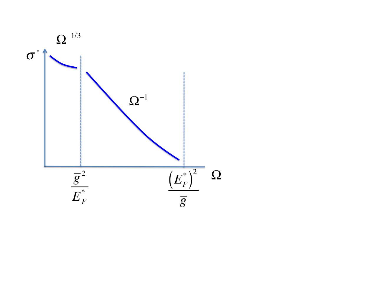
To two-loop order, Eq. (82) was obtained by HHMS who argued, however, that a singular behavior of the conductivity comes only from $2k_{F}$ scattering, while the forward-scattering contribution is canceled by vertex corrections. Our analysis does not reveal major differences between forward- and $2k_{F}$ scattering to two-loop order.

We should point out, however, that the reasoning based on the Boltzmann equation is not precise. While the canonical form of the Boltzmann equation is valid only to second order in a static interaction (or else for an effective interaction obtained in the Random Phase Approximation),[48] scattering at composite bosons corresponds to fourth order in the dynamic interaction–the staggered spin susceptibility. Our situation, however, is simplified by the fact that the intermediate fermions are far off their mass shells. As a result, the four-leg vertex, which should a priori depend on all three fermionic frequencies (the fourth one is fixed by energy conservation), actually depends only on the frequency transfer. For such a vertex, cancelations between the diagrams occur in the same way as predicted by the Boltzmann equation. In the next section, we will present a detailed analysis of the diagrams for the conductivity which confirms the qualitative arguments given in this section.

III.3 Diagrams for the conductivity

III.3.1 Terminology and notations

We use the Kubo formula for the conductivity at finite frequency $\sigma^{\prime}_{jj}(\Omega)\propto\mathrm{Im}{\cal P}_{jj}(\Omega)/\Omega$ . The current-current correlator ${\cal P}_{jj}(\Omega)\equiv{\cal P}(\Omega)$ is given by a particle-hole bubble with zero momentum transfer and frequency transfer $\Omega$ , and with velocities of internal fermions ${\bf v}({\bf p})$ at the vertices.

The two diagrams for the current-current correlator ${\cal P}(\Omega)$ with self-energy insertions are shown in Fig. 12 A. Other contributions to ${\cal P}(\Omega)$ are the vertex-correction diagram (Fig.12 B) and two Aslamazov-Larkin diagrams (Fig. 13) (see, e.g., Ref. 49). Depending on whether the momenta on the solid and dashed are near the same or opposite hot spot, we are dealing with a forward or $2k_{F}$ scattering process, correspondingly.

Before we proceed further, a brief remark on terminology is in order. We believe that the diagram identified by HHMS as a “vertex correction” is actually the first of the two Aslamazov-Larkin diagrams (Fig. 13 C), while the actual vertex-correction diagram (Fig. 12 B ) was not considered by HHMS. We will use this terminology throughout the rest of this section.

Our analysis proceeds in two steps. First, in Sec. III.3.2, we show that diagrams $A$ and $B$ in Fig. 12, as well as diagrams $C$ and $D$ in Fig. 13, cancel each other if one neglects the variations of the $Z$ factor around the FS. Next, in Sec. III.3.3, we show that allowing for the variation of the $Z$ factor prevents complete cancelation and does lead to power-law singularities in the conductivity, as announced in Eqs. (82 and (83).

III.3.2 Cancellation of diagrams under the conditions of strict forward- and $2k_{F}$ -scattering

It is convenient to consider mutual cancelations between the diagrams in Fig. 12 and Fig. 13 separately.

Figure 12: Diagrams for the conductivity. Labels

1

and

\bar{1}

corresponds to hot spots in Fig. 1.

Q_{0}=({\bf 0},\Omega)

is the

(2+1)

momentum of the external electric field. A) Self-energy diagrams. B) Vertex-correction diagram.

Figure 13: Aslamazov-Larkin diagrams for the conductivity. Notations are the same as in Fig. 12.

As before, we use $(2+1)$ notations for the energy and momentum, such that $P=({\bf p},\Omega_{p})$ , etc. The external $(2+1)$ momentum has only the frequency component: $Q_{0}\equiv({\bf 0},\Omega)$ , where $\Omega$ is the frequency of the external electric field (chosen to be positive for convenience.)

Self-energy and vertex-correction diagrams.

First, we discuss the diagrams $A$ and $B$ , whose contributions to the current-current correlator are given by


$\displaystyle{\cal P}_{A}$	$\displaystyle=$	$\displaystyle-\int_{P}{\bf v}_{j}^{2}({\bf p})\left[G(P-Q_{0})G(P)+G(P)G(P+Q_{0})\right]$	(84a)
		$\displaystyle\times G(P)\Sigma(P)$	(84a)
$\displaystyle{\cal P}_{B}$	$\displaystyle=$	$\displaystyle\int_{P\dots K^{\prime}}{\bf v}_{j}({\bf p})\cdot{\bf v}_{j}({\bf p}^{\prime})G(P)G(P+Q_{0})$	(84b)
		$\displaystyle\times G(P^{\prime})G(P^{\prime}+Q_{0})G(K)G(K^{\prime})\Gamma\Gamma_{Q_{0},1},$	(84b)

where


$\displaystyle\Gamma$	$\displaystyle\equiv$	$\displaystyle\Gamma\left(P,K;P^{\prime},K^{\prime}\right),$	(85a)
$\displaystyle\Gamma_{\Omega,1}$	$\displaystyle\equiv$	$\displaystyle\Gamma\left(P+Q_{0},K;P^{\prime}+Q_{0},K^{\prime}\right),$	(85b)

while the self-energy reads

\Sigma(P)=-\int_{P^{\prime},K,K^{\prime}}\Gamma^{2}G(P^{\prime})G(K)G(K^{\prime}).

(86)

For the time being, we are not specifying a particular form of the interaction vertex. The only requirement we impose is that the vertex satisfies the microscopic reversibility condition: $\Gamma(P,K;P^{\prime},K^{\prime})=\Gamma(P^{\prime},K^{\prime};P,K)$ , which we have already used in Eq. (86). Note that the velocities ${\bf v}({\bf p})$ and ${\bf v}({\bf p}^{\prime})$ in Eqs. (84a) and (84b), as well as all velocities in the formulas below, are the bare ones. [50] Velocity renormalization by the interaction is accounted for by the $Z$ factors which occur explicitly in the Kubo formalism.

The Green’s functions in the diagrams $A-D$ are renormalized by ${\bf q}_{\pi}$ scattering, which determines the $Z$ factor. Therefore, the “bare” Green’s functions in the diagrams $A-D$ are of the form

G(P)=\left(\frac{i\Omega_{p}}{Z_{{\bf p}}}-\varepsilon_{{\bf p}}\right)^{-1},

(87)

with $Z_{\bf p}$ given by Eq. (17). Green’s functions of the form (87) satisfy the following identity

G(P)G(P+Q_{0})=\frac{Z_{{\bf p}}}{i\Omega}\left[G(P)-G(P+Q_{0})\right].

(88)

Splitting the products of the Green’s functions in Eq. (84a) with the help of this identity, we re-write ${\cal P}_{A}$ as

{\cal P}_{A}=\frac{1}{i\Omega}\int_{P}{\bf v}_{j}^{2}({\bf p})Z_{{\bf p}}\left[\Sigma(P)-\Sigma(P+Q_{0})\right]G(P)G(P+Q_{0}).

(89)

As we saw in Sec. III.1, the diagram $A$ by itself produces singular terms in the conductivity, given by Eqs. (74-75). By construction, the momenta along both the top and bottom lines of the composite vertex $\Gamma(P,K;P^{\prime},K^{\prime})$ are close to each other, i.e., ${\bf k}^{\prime}\approx{\bf k}$ and ${\bf p}^{\prime}\approx{\bf p}$ , and so are the velocities in diagram $B$ : ${\bf v}({\bf p})\approx{\bf v}({\bf p}^{\prime})$ . To see if the singular contributions from diagrams $A$ and $B$ cancel each other, we first neglect the differences between ${\bf v}({\bf p})$ and ${\bf v}({\bf p}^{\prime})$ , and also between $Z_{\bf p}$ and $Z_{{\bf p}^{\prime}}$ . The first constraint corresponds to either strict forward scattering, when the momenta on the solid and dashed lines are near the same hot spot, or to strict $2k_{F}$ scattering, when these momenta are near the opposite hot spots. The constraint $Z_{\bf p}=Z_{{\bf p}^{\prime}}$ will be relaxed in the Sec. III.3.3. Imposing these constraints and applying identity (88) to the product $G(P^{\prime})G(P^{\prime}+Q_{0})$ in diagram $B$ , we re-write ${\cal P}_{B}$ as

\displaystyle{\cal P}_{B}

\displaystyle=

\displaystyle\frac{1}{i\Omega}\int_{P\dots K^{\prime}}{\bf v}_{j}^{2}({\bf p})Z_{\bf p}\left[G(P)G(P+Q_{0})G(P^{\prime})\Gamma\Gamma_{\Omega,1}-G(P)G(P+Q_{0})G(P^{\prime}+Q_{0})\Gamma\Gamma_{\Omega,1}\right]G(K)G(K^{\prime}).

(90)

Next, we re-write $\Gamma\Gamma_{\Omega,1}$ entering the first and second terms in the square brackets of Eq. (90) as $\Gamma\Gamma_{\Omega,1}+\Gamma^{2}-\Gamma^{2}$ and $\Gamma\Gamma_{\Omega,1}+\Gamma_{\Omega,1}^{2}-\Gamma_{\Omega,1}^{2}$ , correspondingly. Then ${\cal P}_{B}$ can be represented as a sum of three terms: ${\cal P}_{B}={\cal P}_{B}^{1}+{\cal P}_{B}^{2}+{\cal P}_{B}^{3}$ , where


$\displaystyle{\cal P}^{1}_{B}$	$\displaystyle=$	$\displaystyle\frac{1}{i\Omega}\int_{P\dots K^{\prime}}{\bf v}_{j}^{2}({\bf p})Z_{{\bf p}}\left[\Gamma^{2}G(P^{\prime})-\Gamma_{\Omega,1}^{2}G(P^{\prime}+Q_{0})\right]$	(91a)
		$\displaystyle\times G(P)G(P+Q_{0})G(K)G(K^{\prime}),$	(91a)
$\displaystyle{\cal P}^{2}_{B}$	$\displaystyle=$	$\displaystyle\frac{1}{i\Omega}\int_{P\dots K^{\prime}}{\bf v}_{j}^{2}({\bf p})Z_{{\bf p}}\Gamma\left[\Gamma_{\Omega,1}-\Gamma\right]$	(91b)
		$\displaystyle\times G(P^{\prime})G(P)G(P+Q_{0})G(K)G(K^{\prime}),$	(91b)
$\displaystyle{\cal P}^{3}_{B}$	$\displaystyle=$	$\displaystyle\frac{1}{i\Omega}\int_{P\dots K^{\prime}}{\bf v}_{j}^{2}({\bf p})Z_{{\bf p}}\Gamma_{\Omega,1}\left[\Gamma_{\Omega,1}-\Gamma\right]$
		$\displaystyle\times G(P^{\prime}+Q_{0})G(P)G(P+Q_{0})G(K)G(K^{\prime}).$

Using the self-energy from Eq. (86), we re-write ${\cal P}^{1}_{B}$ as

{\cal P}^{1}_{B}=\frac{1}{i\Omega}\int_{P}{\bf v}_{j}^{2}({\bf p})Z_{{\bf p}}\left[\Sigma(P+Q_{0})-\Sigma(P)\right]G(P)G(P+Q_{0}).

(92)

Comparing this result with $P_{A}$ in Eq. (89) we see that this part of the diagram $B$ cancels out the entire diagram $A$ : ${\cal P}_{A}+{\cal P}_{B}^{1}=0$ .

If $\Gamma$ were an arbitrary dynamic vertex, each of the two remaining terms, ${\cal P}^{2}_{B}$ and ${\cal P}_{B}^{3}$ , would, in general, be of the same order as ${\cal P}_{A}$ . Our case, however, is special in the sense that, within the approximation adopted for the composite vertex in Sec. II.3.1, the frequency dependence of $\Gamma(P,K;P^{\prime},K^{\prime})$ involves only one variable – the difference of the frequencies of the initial and final states:

	$\displaystyle\Gamma(P,K;P^{\prime},K^{\prime})=F(\|\Omega_{p}-\Omega_{p^{\prime}}\|;{\bf p}-{\bf p}^{\prime},{\bf p},{\bf k}^{\prime}),$
			(93)

where an explicit form of the function $F$ can be read off from Eq. (23). Since $\Gamma_{\Omega 1}$ differs from $\Gamma$ only by a shift of the initial and final frequencies by $\Omega$ [see Eqs. (85a) and (85b)], it follows from Eq. (93) that $\Gamma_{\Omega,1}=\Gamma$ , and thus ${\cal P}^{2}_{B}={\cal P}^{3}_{B}=0$ . Therefore, the sum of diagrams $A$ and $B$ is equal to zero.

Aslamazov-Larkin diagrams.

We now turn to Aslamazov-Larkin diagrams $C$ and $D$ in Fig. 13. The corresponding contributions to the current-current correlator are:


$\displaystyle{\cal P}_{C}=\int_{P\dots K^{\prime}}$	$\displaystyle{\bf v}_{j}({\bf p})\cdot{\bf v}_{j}({{\bf k}^{\prime}})G(P)G(P+Q_{0})G(K^{\prime})$	(94a)
	$\displaystyle\times G(K^{\prime}+Q_{0})G(P^{\prime})G(K)\Gamma_{\Omega,2}\Gamma,$	(94a)
$\displaystyle{\cal P}_{D}=\int_{P\dots K^{\prime}}$	$\displaystyle{\bf v}_{j}({\bf p})\cdot{\bf v}_{j}({{\bf k}})G(P)G(P+Q_{0})G(K)$
	$\displaystyle\times G(K+Q_{0})G(P^{\prime})G(K^{\prime})\Gamma_{\Omega,3}\Gamma_{\Omega,4}\;,$

where $\Gamma$ is given by Eq. (85a), and


$\displaystyle\Gamma_{\Omega,2}$	$\displaystyle\equiv$	$\displaystyle\Gamma(P+Q_{0},K;P^{\prime},K^{\prime}+Q_{0}),$	(95a)
$\displaystyle\Gamma_{\Omega,3}$	$\displaystyle\equiv$	$\displaystyle\Gamma(P,K+Q_{0};P^{\prime},K^{\prime}),$	(95b)
$\displaystyle\Gamma_{\Omega,4}$	$\displaystyle\equiv$	$\displaystyle\Gamma(P+Q_{0},K;P^{\prime},K^{\prime}).$	(95c)

In each vertex, the sum of the incoming momenta/frequencies is equal to the sum of the outgoing ones. For a forward-scattering process, all momenta in the diagrams $C$ and $D$ are close to each other, i.e., ${\bf p}\approx{\bf p}^{\prime}\approx{\bf k}\approx{\bf k}^{\prime}$ . For a $2k_{F}$ process, the momenta are related to each other as ${\bf p}\approx{\bf p}^{\prime}\approx-{\bf k}\approx-{\bf k}^{\prime}$ . Accordingly, the current vertices can be simplified as

{\bf v}_{j}({\bf p})\cdot{\bf v}_{j}({{\bf k}})={\bf v}_{j}({\bf p})\cdot{\bf v}_{j}({{\bf k}^{\prime}})=\pm{\bf v}^{2}_{j}({\bf p}),

(96)

where the $+$ ( $-$ ) sign corresponds to forward ( $2k_{F}$ ) scattering. As it was done for the diagrams $A$ and $B$ , we also set all the $Z$ factors to be equal to $Z_{\bf p}$ for the time being. Applying identity (88) to the products of the first four Green’s functions in Eqs. (94a) and (), we represent both ${\cal P}_{C}$ and ${\cal P}_{D}$ as a sum of four terms:


$\displaystyle{\cal P}_{C}$	$\displaystyle=$	$\displaystyle\pm\frac{1}{\Omega^{2}}\int_{P,P^{\prime},K,K^{\prime}}\left\{{\bf v}^{2}_{j}({\bf p})Z^{2}_{\bf p}\left[{G(P)G(K^{\prime})}+G(P+Q_{0})G(K^{\prime}+Q_{0})-{G(P)G(K^{\prime}+Q_{0})}-{G(P+Q_{0})G(K^{\prime})}\right]\right.$	(97a)
		$\displaystyle\times G(P^{\prime})G(K)\Gamma\Gamma_{\Omega,2}\Big\}$	(97a)
$\displaystyle{\cal P}_{D}$	$\displaystyle=$	$\displaystyle\pm\frac{1}{\Omega^{2}}\int_{P,P^{\prime},K,K^{\prime}}\left\{{\bf v}^{2}_{j}({\bf p})Z^{2}_{\bf p}\left[{G(P)G(K)}+{G(P+Q_{0})G(K+Q_{0})}-{G(P)G(K+Q_{0})}-{G(P+Q_{0})G(K)}\right]\right.$	(97b)
		$\displaystyle\times G(P^{\prime})G(K^{\prime})\Gamma_{\Omega,3}\Gamma_{\Omega,4}\Big\}.$	(97b)

Shifting the momenta by the external momentum $Q_{0}$ , we reduce the sum of Eqs. (97a) and (97b) to the following form

	$\displaystyle{\cal P}_{C}+{\cal P}_{D}=\pm\frac{1}{\Omega^{2}}\int_{P,P^{\prime},K,K^{\prime}}$		$\displaystyle{\bf v}^{2}({\bf p})Z_{\bf p}^{2}G(P)G(K^{\prime})G(P^{\prime})G(K)$		(98)
			$\displaystyle\times{\cal G}(P,K,P^{\prime},K^{\prime},Q_{0}),$		(98)

where ${\cal G}(P,K^{\prime},P^{\prime},K,Q_{0})$ is a bilinear combination of the vertices given by

$\displaystyle{\cal G}(P,K,P^{\prime},K^{\prime},Q_{0})$	$\displaystyle=$	$\displaystyle\Gamma(P,K;P^{\prime},K^{\prime})\left[\Gamma(P+Q_{0},K;P^{\prime},K^{\prime}+Q_{0})-\Gamma(P+Q_{0},K-Q_{0};P^{\prime},K^{\prime})\right]$	(99)
		$\displaystyle+\Gamma(P,K;P^{\prime},K^{\prime})\left[\Gamma(P-Q_{0},K;P^{\prime},K^{\prime}-Q_{0})-\Gamma(P-Q_{0},K+Q_{0};P^{\prime},K^{\prime})\right]$
		$\displaystyle+\Gamma(P-Q_{0},K;P^{\prime},K^{\prime})\left[\Gamma(P,K-Q_{0};P^{\prime},K^{\prime})-\Gamma(P,K;P^{\prime},K^{\prime}+Q_{0})\right]$
		$\displaystyle+\Gamma(P+Q_{0},K;P^{\prime},K^{\prime})\left[\Gamma(P,K+Q_{0};P^{\prime},K^{\prime})-\Gamma(P,K;P^{\prime},K^{\prime}-Q_{0})\right].$

Again, if $\Gamma$ were an arbitrary vertex, ${\cal G}$ would be non-zero. However, for our form composite vertex, the vertices in each of the four square brackets in Eq. (99) cancel each other. For example, in the first line of Eq. (99) we have $\Gamma(P+Q_{0},K;P^{\prime},K^{\prime}+Q_{0})=F(|\Omega_{p}+\Omega-\Omega_{p^{\prime}}|,{\bf p}-{\bf p}^{{}^{\prime}},{\bf p},{\bf k})$ and $\Gamma(P+Q_{0},K+Q_{0};P^{\prime},K^{\prime})=F(|\Omega_{p}+\Omega-\Omega_{p^{\prime}}|,{\bf p}-{\bf p}^{{}^{\prime}},{\bf p},{\bf k})$ , i.e., the two vertices are equal. Likewise, the remaining three lines in Eq. (99) also vanish. Therefore, ${\cal G}=0$ and ${\cal P}_{C}+{\cal P}_{D}=0$ .

Therefore, if one focuses on strict forward and $2k_{F}$ scattering and neglects the variation of the $Z$ factor along the FS, the contributions to the conductivity from all the diagrams cancel each other.

III.3.3 Absence of cancelation of the power-law singularity in the conductivity

We are now relaxing the constraints of strict forward- and $2k_{F}$ -scattering by taking into account that the $Z$ factors of fermions with different, albeit close, momenta are different. The bare fermionic velocities will be still taken at either the same or opposite; however, as explained in Sec. III.2, the renormalized velocities which, in our model, differ from the bare ones by the $Z$ factors, vary rapidly near the hot spots. Since allowing for such a variation will be already sufficient for eliminating the cancelation of the diagrams even for the special form of the composite vertex in Eq. (93), we initially restrict our analysis to that form of the vertex. Consequently, the vertices entering the diagrams $A$ - $D$ are related to each other as

\Gamma_{\Omega,1}=\Gamma_{\Omega,3}=\Gamma;\;\Gamma_{\Omega,4}=\Gamma_{\Omega,2}.

(100)

With these constraints on the vertices and also with ${\bf v}_{j}({\bf p})={\bf v}_{j}({\bf p}^{\prime})$ , the sum of the diagrams $A$ and $B$ is reduced to

	$\displaystyle{\cal P}_{A}+{\cal P}_{B}$	$\displaystyle=$	$\displaystyle\frac{1}{i\Omega}\int_{P\dots K^{\prime}}{\bf v}^{2}_{j}({\bf p})G(P)G(P+Q_{0})G(K)G(K^{\prime})$		(101)
			$\displaystyle\times\Gamma^{2}\left(Z_{{\bf p}^{\prime}}-Z_{{\bf p}}\right)\left[G(P^{\prime})-G(P^{\prime}+Q_{0})\right].$		(101)

We define the “auxiliary self-energy” as

\Sigma_{Z}(P)\equiv-\int_{P^{\prime},K,K^{\prime}}\Gamma^{2}G(P^{\prime})G(K)G(K^{\prime})\frac{Z_{{\bf p}^{\prime}}}{Z_{{\bf p}}},

(102)

which differs from the usual self-energy [Eq. (86)] by the ratio of the $Z$ factors under the integral. Defining also the difference of the usual and auxiliary self-energies, $\Delta\Sigma(P)\equiv\Sigma(P)-\Sigma_{Z}(P)$ , we re-write Eq. (101) as

	$\displaystyle{\cal P}_{A}+{\cal P}_{B}$	$\displaystyle=$	$\displaystyle\frac{1}{i\Omega}\int_{P}{\bf v}^{2}_{j}({\bf p})Z_{\bf p}\left[\Delta\Sigma(P)-\Delta\Sigma(P+Q_{0})\right]$		(103)
			$\displaystyle\times G(P)G(P+Q_{0}).$		(103)

Now the sum of the diagrams $A$ and $B$ has a form similar to that of the diagram $A$ itself [Eq. (89)], except for the usual self-energy in Eq. (89) is replaced by $\Delta\Sigma$ in Eq. (103). Therefore, to compare Eqs. (89) and (103), we only need to compare the two-loop self-energy with

	$\displaystyle\Delta\Sigma(K)=-\int_{P,P^{\prime},K^{\prime}}\Gamma^{2}G(P)G(P^{\prime})G(K^{\prime})\frac{Z_{{\bf k}}-Z_{{\bf k}^{\prime}}}{Z_{{\bf k}}}.$
			(104)

In what follows, we consider explicitly only the 2D regime of two-loop composite scattering with the self-energy given by Eq. (31). When evaluating the usual self-energy in Eq. (29), we integrated over $p_{\perp}$ and then over $q_{\perp}$ , which led us to Eq. (30). Performing the same integrations in Eq. (104) and using an explicit form of the $Z$ -factor from Eq. (17), we arrive at

	$\displaystyle\Delta\Sigma_{\mathrm{comp}_{2}}(\delta k,\Omega_{k})$	$\displaystyle=$	$\displaystyle\frac{1}{2v_{F}}\int\frac{d\Omega_{q}}{2\pi}\int\frac{d\delta q}{2\pi}\int\frac{d\Omega_{p}}{2\pi}\int\frac{d\delta p}{2\pi}\frac{\mathrm{sgn}(\Omega_{p}-\Omega_{q})-\mathrm{sgn}(\Omega_{p})}{\frac{{i\Omega_{p}}}{Z_{\bf p}}-\frac{i(\Omega_{p}-\Omega_{q})}{Z_{{\bf p}-{\bf q}}}-\frac{\delta p\delta q}{m^{}}+\frac{(\delta q)^{2}}{2m^{}}}{\cal Z}_{\delta k,\delta q}$		(105)
			$\displaystyle\times\mathrm{sgn}(\Omega_{k}+\Omega_{q})\Gamma^{2}(K,P;Q).$		(105)

where ${\cal Z}_{\delta k,\delta q}\equiv 1-|\delta k+\delta q|/|\delta k|$ . Since ${\cal Z}_{\delta k,\delta q}$ vanishes as $\delta q$ at $\delta q\to 0$ , the $1/|\delta q|$ singularity of the particle-hole bubble is eliminated. In the absence of the $1/\delta q$ singularity, the internal momenta are of order of the internal one: $\delta q\sim\delta p\sim\delta k$ . Therefore, the logarithmic factor in the vertex [Eq. (23)] is replaced by a number of order one, whereas the third (kinematic) logarithm simply does not occur. As a result, $\Delta\Sigma$ contains no logarithmic factors. However, ${\cal Z}_{\delta k,\delta q}\sim 1$ at relevant $\delta q\sim\delta k$ and thus does not affect power-counting of the rest of the result, which reads

\Delta\Sigma^{\prime\prime}\sim\Omega^{2}\frac{{\bar{g}}^{2}}{(v_{F}\delta k)^{3}}\frac{E^{*}_{F}}{v_{F}\delta k}.

(106)

Therefore, the combined contribution of the diagrams $A$ and $B$ differs only by a logarithmic factor from the self-energy contribution (the diagram $A$ ).

The imaginary parts of the self-energies two-loop composite scattering in the 1D regime [Eq. (40)] and from ${\bf q}_{\pi}$ scattering of hot fermions [Eq. (14) with $\delta k=0$ ] contain no logarithmic factors. Since ${\cal Z}_{\delta k,\delta q}\sim 1$ in these cases as well, the combined contribution of the diagrams $A$ and $B$ differs from that of the diagram $A$ only by a number of order one.

We now turn to the diagrams $C$ and $D$ . Using constraints (100) for the interaction vertices and (96) for the current vertices but keeping the momentum dependence of the $Z$ -factors, we obtain for the sum of the diagrams $C$ and $D$

	$\displaystyle{\cal P}_{C}+{\cal P}_{D}=\pm\frac{1}{i\Omega}\int_{P\dots K^{\prime}}{\bf v}^{2}_{j}({\bf p})\Gamma\Gamma_{\Omega,2}\left(Z_{{\bf k}}-Z_{{\bf k}^{\prime}}\right)\left[G(K)G(K^{\prime}+Q_{0})G(P^{\prime})-G(K)G(K^{\prime})G(P^{\prime})\right]G(P)G(P+Q_{0}).$
			(107)

[In deriving this result, we also used properties (88) and (93).] In general, Eq. (107) cannot be expressed via the self-energy because it contains a product of different interaction vertices, $\Gamma$ and $\Gamma_{\Omega,2}$ , whereas the self-energy contains $\Gamma^{2}$ , and also because the external frequency enters the first term in the square brackets in a different way as compared to the self-energy diagram. In our case, however, these differences are immaterial. Indeed, Eq. (95a) shows that $\Gamma_{\Omega,2}$ differs from $\Gamma$ only in that the first and last fermionic frequencies are shifted by the external frequency $\Omega$ . Since the composite vertex in Eq. (23) depends on the frequency only logarithmically, the difference between $\Gamma$ and $\Gamma_{\Omega_{2}}$ is not important to logarithmic accuracy. If we identify $\Gamma$ with $\Gamma_{\Omega,2}$ , the second term in the square brackets, taken without the $(Z_{\bf k}-Z_{{\bf k}^{\prime}})$ factor, reduces to $\Sigma(P)$ . As it was the case for the sum of diagrams $A$ and $B$ , the role of the $(Z_{\bf k}-Z_{{\bf k}^{\prime}})$ factor is to regularize the $1/\delta q$ singularity of the particle-hole bubble. After this regularization, the second term in the square brackets gives the same contribution to the conductivity as the self-energy diagram without an extra logarithm.

In the first term, the frequency of the fermion $K^{\prime}$ is shifted by the external frequency. Denoting again $K^{\prime}=K+Q$ and $P^{\prime}=P-Q$ , it is easy to see that this shift changes the frequency of the particle-hole bubble formed by fermions $K$ and $K+Q+Q_{0}$ , such that instead of $|\Omega_{q}|/|\delta q|$ we now have $|\Omega_{q}+\Omega|/|\delta q|$ . The change has the same effect as shifting the frequency of the incoming fermion from $\Omega_{p}$ to $\Omega_{p}+\Omega$ : the $(Z_{\bf k}-Z_{{\bf k}^{\prime}})$ factor again removes one of the logarithms.

We thus see that the combined contribution of diagrams $C$ and $D$ is of the same order as that of diagrams $A$ and $B$ . The two groups of diagrams cancel each other to leading logarithmic order. Beyond this order, however, the vertices in diagrams $C$ and $D$ differ from those in $A$ and $B$ , and thus a cancelation cannot happen. We therefore conclude, that the sum of the four diagrams differs from the self-energy diagram by at most a logarithmic factor, and the conductivity does indeed scale as announced in Eqs. (82) and (83).

III.3.4 Subleading non-singular terms in the optical conductivity

For completeness, we also analyze the form of the subleading terms in the optical conductivity, which are present even under the assumptions adopted in Sec. III.3.2, i.e., strict forward- and $2k_{F}$ -scattering and constant $Z$ factor. These subleading terms appear because the diagrams for the conductivity do not cancel each other if the frequency dependence of the composite vertex is taken into account. Indeed, when deriving Eq. (23) we approximated the fermionic propagator $G(K+Q_{\pi})$ by its static form ( $-1/v_{F}\delta p$ ), and similarly for the second propagator, $G(P+Q_{\pi})$ . The full fermionic propagator depends on the frequency via the $\Omega_{k}/Z_{{\bf k}}$ term. All internal frequencies in the diagrams for ${\cal P}$ are of order $\Omega$ , hence the extra terms which distinguish between, e.g., $\Gamma_{\Omega,1}$ and $\Gamma$ , come in powers of $\Omega/Z_{\bf k}v_{F}\delta k\propto\Omega/\delta k|\delta k|$ , where we used that $Z_{\bf k}\propto|\delta k|$ for lukewarm fermions. The first-order term again vanishes by parity, and the leading term in $\Gamma_{\Omega,1}-\Gamma$ scales as $\Gamma\Omega^{2}/(\delta k)^{4}$ . In the 2D regime of composite scattering, typical $|\delta k|\propto\Omega^{1/3}$ , hence the extra term is of order $\Omega^{2/3}$ , and the corresponding contribution to conductivity scales as $\Omega^{1/3}$ , i.e., $\sigma^{\prime}(\Omega)\sim\mathcal{O}(\Omega^{-1/3})+\mathcal{O}(\Omega^{1/3})$ . This dependence is non-analytic yet subleading to a constant, FL term in the conductivity. In the 1D regime, typical $\delta k$ are frequency independent, hence the correction to the conductivity scales as $\Omega^{2}$ , i.e., $\sigma^{\prime}(\Omega)\sim\mathcal{O}(\Omega^{-1})+\mathcal{O}(\Omega^{2})$ .

IV Conclusions

In this paper, we considered the $T=0$ optical conductivity of a clean two-dimensional metal near a spin-density-wave instability with momentum ${\bf q}_{\pi}=(\pi,\pi)$ . It is well established by now that critical magnetic fluctuations destroy fermionic coherence in hot regions, but coherent quasiparticles survive on the rest of the FS. Recent analysis by HHMS (Ref. 21) has demonstrated that the contribution to the conductivity from hot fermions is reduced by vertex corrections, and is subleading to a constant, Fermi-liquid contribution from cold fermions. These authors also argued that composite scattering between lukewarm fermions (which behave as Fermi-liquid albeit strongly renormalized quasiparticles) gives a singular contribution to the conductivity because the diagrams with self-energy and vertex-correction insertions do not cancel each other.

We found that the imaginary part of the fermionic self-energy from two-loop composite scattering scales as $\Sigma^{\prime\prime}({\bf k}_{F},\Omega)\propto\Omega^{2}/\delta k^{4}\ln^{3}{|v_{F}\delta k/\Omega|}$ , for $\Omega$ below some characteristic scale, and as $\Omega\min\{v_{F}\delta k/{\bar{g}},1\}/\delta k^{2}$ , above that scale. The conductivity obtained by inserting such a self-energy into the current-current correlator exhibits a NFL, singular dependence on $\Omega$ : $\sigma^{\prime}_{\Sigma}(\Omega)\propto\ln^{3}\Omega/\Omega^{1/3}$ and $\sigma^{\prime}_{\Sigma}(\Omega)\propto 1/\Omega$ for $\Omega$ below and above $\Omega_{\min}={\bar{g}}^{2}/E_{F}$ , correspondingly. At the high-frequency end, the $1/\Omega$ scaling of $\sigma^{\prime}_{\Sigma}(\Omega)$ extends all the way up to the bandwidth, above which the low-energy theory becomes inapplicable.

We showed that the vertex-correction and Aslamazov-Larkin diagrams cancel out a part of but not all the self-energy contribution. Namely, the low-frequency form of the full conductivity loses the logarithmic prefactor but retains a power-law, $\Omega^{-1/3}$ singularity, whereas the high-frequency, $1/\Omega$ form remains intact (up to a number). The full conductivity behaves as specified by Eq. (I.2).

As a word of caution, Eq. (I.2) is only a two-loop result. As shown in Sec. II.6, corrections to the self-energy from higher loops are of the same order as the two-loop result at lower frequencies and are formally larger than the two-loop result by a logarithmic factor at higher frequencies. This means, in particular, that the scaling form of the conductivity in the high-frequency regime should acquire an anomalous exponent: $\sigma^{\prime}(\Omega)\propto 1/\Omega\to\sigma^{\prime}(\Omega)\propto 1/\Omega^{1+\beta}$ . A calculation of $\beta$ requires non-perturbative methods and is beyond the scope of this paper.

We emphasize that non-analytic terms in the conductivity, considered in this paper, are different from the ones in the presence of impurities.[51] In the latter case, non-analytic terms appear as corrections to a constant Drude term due to impurity scattering and predominantly come from hot fermions. We caution, however, that a computation of the conductivity in near-critical dirty systems requires a special care. [52]

Strictly speaking, the range for the $1/\Omega$ scaling of $\sigma^{\prime}(\Omega)$ is well-defined only under the assumption that the spin-fermion coupling is weak, i.e., $\bar{g}<E_{F}$ . The actual behavior of $\sigma^{\prime}(\Omega)$ is determined by the numerical coefficients which are hard to calculate in a consistent way. It is still encouraging, however, to see that a microscopic model predicts a $1/\Omega$ scaling in a (at lest formally) wide frequency range, which is consistent with the behavior observed in the cuprates.[10] The scale $\Omega_{\min}\sim{\bar{g}}^{2}/E_{F}$ is parametrically smaller than the scale of the superconducting $T_{c}\sim{\bar{g}}$ , hence $1/\Omega^{1/3}$ behavior is likely to be masked by superconductivity (or finite $T>T_{c}$ ).

An interesting question to be addressed elsewhere is whether there is $\Omega/T$ scaling of the conductivity and, in particular, whether the $1/\Omega$ behavior of the conductivity at $T=0$ is paralleled by a the linear-in- $T$ behavior of the resistivity in a similarly wide temperature range.

Acknowledgements.

We thank J. Betouras, S. Hartnoll, S. Kivelson, G. Kotliar, S. Maiti, M. Metlitski, I. Paul, S. Sachdev, and P. Wölfle for fruitful discussions. We are particularly thankful to M. Metlitski for critical comments on the first version of the manuscript. This work was supported by the Department of Energy via grant No. DE-FG02-ER46900 (A.V.C.), National Science Foundation via grant No. DMR-1308972 (D.L.M.), and Russian Foundation for Basic Research via grant No. 12-02-00100 (V.I.Y.). D.L.M. and A.V.C. thank the Aspen Center for Physics and MPIPKS (Dresden) for hospitality during the work on this project. The Aspen Center for Physics is supported by the National Science Foundation via grant PHYS-1066293.

References

[1] N. E. Hussey, R. A. Cooper, Xiaofeng Xu, Y. Wang, I. Mouzopoulou, B. Vignolle,and C. Proust, Phil. Trans. R. Soc. A. 369, 1941 (2011).
[2] See J. A. N Bruin, H. Sakai, R. S. Perry, and A. P. Mackenzie, Science 339, 804 (2013), and references therein.
[3] R. Mahajan, M. Barkeshli, S. A. Hartnoll, Phys. Rev. B 88, 125107 (2013).
[4] See, e.g., A. A. Abrikosov, L. P. Gor’kov, and I. E. Dzyaloshinski, Methods of Quantum Field Theory in Statistical Physics, (Dover Publications, New York, 1963); D. Pines and P. Nozieres, The Theory of Quantum Liquids, (Addison-Wesley, Menlo Park, 1966).
[5] L. Taillefer, Ann. Rev. Cond.. Matter Phys. 1, 51 (2010); M.A.Tanatar, N. P. Butch, K. Jin, K. Kirshenbaum, R. L. Greene, and J. Paglione, Proc. Natl. Acad. Sci. 109, 8440 (2012).
[6] A similar behavior with $\rho(T)\propto T^{3/2}$ observed in the helimagnet MnSi under pressure [38] is unlikely to be associated with quantum criticality, as the $T^{3/2}$ behavior is seen in a wide range of pressures above the critical one.
[7] G. Oomi, T. Kagayama, and Y. Onuki, J. Alloys Comp., 271-273, 482 (1998); M. Nicklas, M. Brando, G. Knebel, F. Mayr, W. Trinkl, and A. Loidl, Phys. Rev. Lett. 52, 42684271 (1999); P. G. Niklowitz, F. Beckers, G. G. Lonzarich, G. Knebel, B. Salce, J. Thomasson, N. Bernhoeft, D. Braithwaite, and J. Flouquet, Phys. Rev. B 72, 024424 (2005).
[8] T. Timusk and B. Statt, Rep. Prog. Phys. 62, 61 (1999); D. N. Basov, R. D. Averitt, D. van der Marel, M. Dressel, and K. Haule, Rev. Mod. Phys. 83, 471 (2011).
[9] Recent experiment in the pseudogap region did find a $\max\{\Omega^{2},T^{2}\}$ behavior of the optical scattering rate, reminiscent of a FL; see S. I. Mirzaei, D. Stricker, J. N. Hancock, C. Berth od, A. Georges, E. van Heumen, M. K. Chan, X. Zhao, Y. Li, M. Greven, N. Barišić, and D. van der Marel, Proc. Natl. Acad. Sci. USA 110, 5774 (2013).
[10] A. V. Puchkov et al J. Phys. Chem. Solids 59, 1907 (1998); D. N. Basov R. Liang, B. Dabrovski, D. A. Bonn, W. N. Hardy and T. Timusk, Phys. Rev. Lett. 77, 4090, (1996); A. Puchkov, D. Basov, and T. Timusk, J. Phys.: Condens. Matter 8, 10049 (1996); R. Haslinger, A. V. Chubukov, and Ar. Abanov, Phys. Rev. B 63, 020503 (2000); Ar. Abanov, Andrey V. Chubukov, and J. Schmalian, Phys. Rev. B 63, 180510 (2001).
[11] A. El Azrak, R. Nahoum, N. Bontemps, M. Guilloux-Viry, C. Thivet, A. Perrin, S. Labdi, Z. Z. Li, Z. Z. and H. Raffy, Phys. Rev. B49, 9846 (1994).
[12] D. van der Marel, H. J. A. Molegraaf, J. Zaanen, Z. Nussinov, F. Carbone, A. Damascelli, H. Eisaki, M. Greven, P. H. Kes, and M. Li, Nature (London) 425, 271 (2003).
[13] M. R. Norman and A. V. Chubukov Phys. Rev. B 73, 140501 (2006).
[14] J. S. Dodge, C. P. Weber, J. Corson, J. Orenstein, Z. Schlesinger, J. W. Reiner, and M. R. Beasley, Phys. Rev. Lett. 85, 4932 (2000).
[15] Y. S. Lee, J. Yu, J. S. Lee, T. W. Noh, T. H. Gimm, H.-Y. Choi, and C. B. Eom, Phys. Rev. B 66, 041104(R) (2002).
[16] S. Kamal, D. M. Kim, C. B. Eom, and J. S. Dodge, Phys. Rev. B 74, 165115 (2006).
[17] F. P. Mena, D. van der Marel, A. Damascelli, and M. Fäth, A. A. Menovsky, and J. A. Mydosh, Phys. Rev. B 67, 241101 (2003).
[18] See E. Abrahams and C. Varma, Proc. Natl. Acad. Sci. USA 97, 5714 (2000), and references therein.
[19] R. Hlubina and T. M. Rice, Phys. Rev. B 51, 9253 (1995).
[20] see e.g., A. Shekhter and C. M. Varma, Phys. Rev. B 79, 045117 (2009) and references therein.
[21] S. A. Hartnoll, D. M. Hofman, M. A. Metlitski, and S. Sachdev, Phys. Rev. B 84, 145115 (2011).
[22] A “generic FS” means that it corresponds to a non-quadratic anisotropic dispersion for the 3D case, and is either concave or multiply-connected for the 2D case; see Refs. 24 and 25.
[23] See, e.g., A. J. Schofield, Contemp. Phys. 40, 95 (1999).
[24] A. Rosch and P. C. D. Howell, Phys. Rev. B72, 104510 (2005); A. Rosch, Ann. Phys. 15, 526 (2006);
[25] D. L. Maslov, V. I. Yudson, and A. V. Chubukov, Phys. Rev. Lett. 106, 106403 (2011); H. K. Pal, V. I. Yudson, and D. L. Maslov, Phys. Rev. B 85, 085439 (2012); H. K. Pal, V. I. Yudson, and D. L. Maslov, Lith. J. Phys. 52, 142 (2012).
[26] S-S. Lee, Phys. Rev. B 80, 165102 (2009), S-S. Lee, Y-B. Kim, and A.V. Chubukov (unpublished).
[27] M. A. Metlitski and S. Sachdev, Phys. Rev. B 82, 075128 (2010); New J. Phys. 12, 105007 (2010).
[28] Ar. Abanov, A. V. Chubukov, and J. Schmalian, Adv. Phys. 52, 119 (2003).
[29] See, e.g., B. P. Stojkovic and D. Pines, Phys. Rev. Lett. 76, 811 (1996); B. P. Stojkovic and D. Pines, Phys. Rev. B 55, 8576 (1997); A. T. Zheleznyak, V. Yakovenko, H. D. Drew, and I. I. Mazin, ibid. 57, 3089 (1998); L. B. Ioffe and A. J. Millis, ibid. 58, 11631 (1998); J. Kokalj, N. E. Hussey, R. H. McKenzie, ibid. 86 045132 (2012).
[30] E. Abrahams, J. Schmalian, and P. Wölfle, arXiv:1303.3926.
[31] To be more precise, the initial and the final states belong to the opposite hots spots. Once the fermions at hot spots $2$ and $\bar{2}$ are integrated out, the effective scattering process can be labeled as $(1,\bar{1};1,\bar{1})$ , i.e., the fermions located initially at spots $1$ and $\bar{1}$ remain in the vicinity of their respective hot spots. In the terminology of Ref. 34, such a process can be viewed either as a $q=0$ part of the “backscattering process”, with an amplitude given by the difference of the charge and spin components of the scattering amplitude, or as a special case of a Cooper process, in which the initial fermions with the total momentum close to zero retain their initial momenta.
[32] D. F. Mross, J. McGreevy, H. Liu, and T. Senthil, Phys. Rev. B 82, 045121 (2010).
[33] G. Y. Chitov and A. J. Millis, Phys. Rev. B 64, 054414 (2001).
[34] A. V. Chubukov, D. L. Maslov, S. Gangadharaiah, and L. I. Glazman, Phys. Rev. B71, 205112 (2005).
[35] A. V. Chubukov and D. L. Maslov, Phys. Rev. B68, 155113 (2003).
[36] A. V. Chubukov, D. L. Maslov, and A. J. Millis, Phys. Rev. B73, 045128 (2006)
[37] I. L. Aleiner and K. B. Efetov Phys. Rev. B74, 075102 (2006).
[38] H. v. Löhneysen, A. Rosch, M. Vojta, and P. Wölfle, Rev. Mod. Phys. 79, 1015 (2007).
[39] H. Meier, C. Pèpin, and K. B. Efetov, Phys. Rev. B 84, 205131 (2011).
[40] We thank M. Metlitski for clarifying this point for us.
[41] Yu. A. Bychkov, L. P. GorÕkov, and I. E. Dzyaloshisnkii, Sov. Phys. JETP 23, 489 (1966).
[42] See, e.g., D. L. Maslov, in Nanophysics: Coherence and Transport, edited by H. Bouchiat, Y. Gefen, G. Montambaux, and J. Dalibard, Les Houches, Session LXXXI, 2004 (Elsevier, 2005), p. 1 (arXiv:cond-mat/0506035), and references therein.
[43] T. Giamarchi, Quantum Physics in One Dimension (Oxford, 2004).
[44] A. Imambekov, T. L. Schmidt, and L. I. Glazman, Rev. Mod. Phys. 84, 1253 (2012).
[45] G. Schwiete and K. B. Efetov, Phys. Rev. B 74, 165108 (2006); A. Shekhter and A. M. Finkelstein, Phys. Rev. B 74, 205122 (2006); A. V. Chubukov and D. L. Maslov, Phys. Rev. B 76, 165111 (2007).
[46] We neglect the dependence of the self-energy on $k_{\perp}$ , so that the velocity renormalization factor $(1+\frac{\partial\Sigma^{\prime}}{v_{F}\partial k_{\perp}})(1+\frac{\partial\Sigma^{\prime}}{\partial\Omega})^{-1}\approx(1+\frac{\partial\Sigma^{\prime}}{\partial\Omega})^{-1}$ coincides with the $Z$ factor.
[47] The reduction of the transport scattering rate compared with the quasiparticle decay rate due to a small $Z$ factor has recently been emphasized in X. Deng, J. Mravlje, R. Zitko, M. Ferrero, G. Kotliar, and A. Georges, Phys. Rev. Lett. 110, 086401 (2013); W. Xu, K. Haule, and G. Kotliar, arXiv:1304.7486.
[48] E. M. Lifshitz and L. P. Pitaevskii, Physical Kinetics (Pergamon Press, Oxford, 1981); J. Rammer and H. Smith, Rev. Mod. Phys. 58, 323 (1986).
[49] A. I. Larkin and A. V. Varlamov, Theory of fluctuations in superconductors, (Oxford University Press, 2005).
[50] In general, the current vertex contains not the bare velocity but rather the “charge” one, which differs from the bare velocity by a factor of $1+\frac{\partial\Sigma^{\prime}}{v_{F}\partial k_{\perp}}$ . [53, 54, 55] In our case, however, this derivative can be neglected (see comment 46), and thus the charge velocity is almost equal to the bare one.
[51] K. Ueda, J. Phys. Soc. Jpn. 43, 1497 (1977); A. Rosch, Phys. Rev. Lett. 82, 4280 (1999); S. V. Syzranov and J. Schmalian, ibid. 109, 156403 (2012).
[52] S. Sachdev, C. Buragohain, and M. Vojta, Science 286, 2479 (1999).
[53] G. M. Eliashberg, Sov. Phys. JETP 14, 886 (1962).
[54] K. Michaeli and A. M. Finkel’stein, Phys. Rev. B80, 115111 (2009)
[55] D. L. Maslov and A. V. Chubukov, Phys. Rev. B 86, 155137 (2012).

Optical conductivity of a two-dimensional metal at the onset of spin-density-wave order

Abstract

I Introduction

I.1 Optical conductivity near a QCP: summary of prior results

I.1.1 Pomeranchuk QCP (q=0q=0)

I.1.2 Density-wave QCP (finite qq)

I.2 Summary of the results of this paper

II Spin-fermion model and fermionic self-energy

II.1 Spin-fermion model

II.2 Self-energy due to 𝐪π{\bf q}_{\pi} scattering

II.2.1 One-loop order

II.2.2 Classification of fermions as “cold”, “lukewarm”, and “hot” in the presence of 𝐪π{\bf q}_{\pi}-scattering

II.2.3 Higher-order terms and the accuracy of the perturbation theory

II.3 Self-energy due to composite scattering

II.3.1 Composite scattering vertex

II.3.2 “One-loop” self-energy due to composite scattering

II.3.3 Two-loop self-energy due to composite scattering

Main features of two-loop composite scattering.

Two-dimensional regime.

One-dimensional regime.

II.4 Fermionic self-energy: Summary of the results

II.5 Classification of fermions as “cold”, “lukewarm”, and “hot” in the presence of composite scattering

II.6 Higher-loop orders in composite scattering

III Optical conductivity at a quantum critical point

III.1 Self-energy contribution to the optical conductivity

III.2 Vertex corrections: Boltzmann equation

III.3 Diagrams for the conductivity

III.3.1 Terminology and notations

III.3.2 Cancellation of diagrams under the conditions of strict forward- and 2​kF2k_{F}-scattering

Self-energy and vertex-correction diagrams.

Aslamazov-Larkin diagrams.

III.3.3 Absence of cancelation of the power-law singularity in the conductivity

III.3.4 Subleading non-singular terms in the optical conductivity

IV Conclusions

Acknowledgements.

References

Optical conductivity of a two-dimensional metal
at the onset of spin-density-wave order

I.1.1 Pomeranchuk QCP ( $q=0$ )

I.1.2 Density-wave QCP (finite $q$ )

II.2 Self-energy due to ${\bf q}_{\pi}$ scattering

II.2.2 Classification of fermions as “cold”, “lukewarm”, and “hot” in the presence of ${\bf q}_{\pi}$ -scattering

III.3.2 Cancellation of diagrams under the conditions of strict forward- and $2k_{F}$ -scattering